Ongoing Tracking of Engagement in Motor Learning

Abstract.

Teaching motor skills such as playing music, handwriting, and driving, can greatly benefit from recently developed technologies such as wearable gloves for haptic feedback or robotic sensorimotor exoskeletons for the mediation of effective human-human and robot-human physical interactions. At the heart of such teacher-learner interactions still stands the critical role of the ongoing feedback a teacher can get about the student’s engagement state during the learning and practice sessions. Particularly for motor learning, such feedback is an essential functionality in a system that is developed to guide a teacher on how to control the intensity of the physical interaction, and to best adapt it to the gradually evolving performance of the learner. In this paper, our focus is on the development of a near real-time machine-learning model that can acquire its input from a set of readily available, noninvasive, privacy-preserving, body-worn sensors, for the benefit of tracking the engagement of the learner in the motor task. We used the specific case of violin playing as a target domain in which data were empirically acquired, the latent construct of engagement in motor learning was carefully developed for data labeling, and a machine-learning model was rigorously trained and validated.

1. Introduction

Our focus in this work is part of an effort to develop innovative instrumentation, which combines hardware and software, with the purpose of physically coupling humans to enhance complex motor skill learning, such as handwriting and music learning. The work is conducted under a project that develops an exoskeleton-based human-human and robot-human interactions for motor learning. Learning to play the violin, as one specific example of a motor skill, is one of the most complex musical instruments to learn (Provenzale and et al., 2021). Such learning relies on physical interactions in which the learner continuously employs sensorimotor haptics to learn from others (Basdogan et al., 2000; Reed and Peshkin, 2008; Ganesh and et al., 2014). The effectiveness of the learner is driven by a variety of factors. Particularly,we attend to the desire of the teacher to be able to adapt their teaching pace and level of difficulty, while continuously ensuring that the learner is in the ‘right’ mental state, an aspect that significantly influences the learning process and the eventual successful completion of a task (Bower, 1992; Martocchio, 1994; Warr and Bunce, 1995). This can be achieved by utilizing wearable sensors as input data to identify users’ mental and emotional status and change the engagement platform’s behavior accordingly. Recent work on human activity and mental state recognition (e.g., fatigue, stress) has most of its focus on leveraging body-worn measurements and extracted features such as gait and breathing patterns using Inertial Motion Units (IMUs), Gyroscope (GYR), Heart-rate Variability (HRV), and Galvanic Skin Response (GSR) (Shaffer and Ginsberg, 2017). Based on such measures, machine-learning models provide insights regarding the physical, mental, and emotional states of the student. Specifically, in this work, our goal is a rigorous methodological development of a classification model for near real-time determination of learners’ engagement in the performance of a motor task, namely Engagement in Motor-learning (EML). We also demonstrate how observational sensor data can be integrated with adequate labeling which is essential for the employment of supervised machine learning. Such labeling was achieved via a behavioral model that was rigorously developed for capturing EML as its latent construct utilizing self-reported scales from violin players. The developed model has its theoretic foundations rooted in the Flow theory (Csikszentmihalyi, 1990). Subsequently, data that were gathered with the behavioral model were further interpolated in the context of each individual excerpt to increase its density and enable the use of supervised ML. This interpolation also promotes the responsiveness of the developed ML model, where we also ensured to not synthetically over-inflate the accuracy of the developed model. Finally, we also examined the performance of the model with respect to subsets of sensor input.

Ultimately, the resulting model developed here will be embedded for ongoing feedback to teachers, and for the control of a modular robotic platform that integrates wearable technology as a feedback mechanism. This integration aims to facilitate more effective human-human and human-robot interaction, driving motor learning activities such as playing music or handwriting. Overall, the result of this work enables the monitoring of the student’s engagement state as a second modality that complements the conventional output of the activity, whether it is vocal as in the case of music playing, or graphical as in the case of handwriting.

2. Related Literature

Recent advances with body-worn sensors have the potential to capture data that may cater to the monitoring of a wide variety of physiological, mental, and emotional conditions. Contemporary machine learning techniques are also well-developed to capture complex, multi-tiered correspondences between such sensor data and mental conditions. Thus, it is essential for the training of such models to combine both, sensor data relevant for the classification task input, and also labeling of the data with the target states to be predicted. It is key to have such data with both ingredients put in sync in our training set for the construction of an accurate classifier.

There is a vast literature on the engagement concept captured via single or multi-sensor instrumentation, with subclassifications split between cognitive and emotional. The concept itself is somewhat vaguely defined, in many cases due to being task-oriented in nature. Prior work features different target activities such as in-class learning (Gao et al., 2022; DiSalvo et al., 2022; Aslan and et al., 2014), learning with VR (Dubovi, 2022), internet web browsing (Bulger and et al., 2008), maker learning (Lee et al., 2019), general task engagement (Fairclough and et al., 2009), and even military operational duties (Berka and et al., 2007). A recent exhaustive survey (Li, 2021) summarizes a plethora of methods for cognitive engagement measurements, including self-report scales, observations, interviews, teacher ratings, experience sampling, eye-tracking, physiological sensors, trace analysis, and content analysis. Specifically, with respect to sensing devices employed for its measurement, GSR and Electromyography (EMG)are determined to be most common for emotional engagement, while Electroencephalogram (EEG)is commonly used for cognitive engagement. EEG is a good solution for highly reliable ongoing measurements, as demonstrated in (Berka and et al., 2007), but it is very tedious to employ. Alternative efforts include less invasive means such as facial expression, eye tracking, GSR, and body posture captured with cameras (e.g., (Dubovi, 2022; Aslan and et al., 2014)), sometimes attempted as a surrogate for IMU motion sensing (Santhalingam et al., 2023).

Different measurements are relevant for the capturing of EML as a specific type of cognitive and emotional manifestation, based on different physiological parameters associated with the Central Nervous System (CNS), and with changes of the Autonomous Nervous System (ANS). Such activity can be analyzed by monitoring electrodermal, respiratory, cardiac, and inertial activities. Galvanic Skin Response (GSR) analysis has been developed to discriminate with good accuracy different levels of arousal (Lanata et al., 2012). Heart Rate Variability (HRV) in both time and frequency domains can provide a noninvasive assessment of ANS function (Rajendra Acharya and et al., 2006). The analysis of HRV nonlinear measures has been found to be important for emotional arousal and valence recognition from ANS signals (Valenza and et al., 2014; Katsis et al., 2011). Similarly, cessation of respiration tracking (e.g., using IMUs) can be associated with stress (Gorman and et al., 2004; Wu et al., 2012).

In our instrumental design, we had to meet specific requirements and accommodate the unique activity of motor learning as our target. Hence, we had to rule out frequent interruptions during the main activity. We also had to ensure that we used readily available, privacy-preserving sensors. This conformed to our intentions to embed them within a broader interaction training platform, destined for deployment in schools or industrial training facilities where privacy is a paramount concern. Our sensor selection also aimed to have a minimal footprint, aiming to minimize discomfort during task performances such as violin playing.

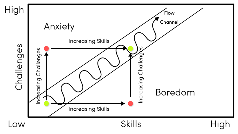
Figure 1. The Flow theory: ‘flow’ is attained when the level of skill matches the perceived complexity of the challenge.

Our aim to measure the condition of being engaged in the performance of a motor task was concretely instantiated by the activity of playing the violin during practice sessions in this work. For this, we adopt from the theory of optimal experience or ‘Flow’ by Csikszentmihalyi (Csikszentmihalyi, 1990), which conceptualizes flow as a state of concentration that amounts to absolute absorption in an activity. It refers to “the state in which people are so involved in an activity that nothing else seems to matter.” Henceforth, matching our concept of EML. Specific to the domain of music, the theory also attributes music itself as auditory information that helps “organize the mind…listening to music wards off boredom and anxiety, and when seriously attended to, it can induce flow experiences…even greater rewards are open to those who learn to make music…” Aside from aiding with the conceptualization of the notion itself, the same theory also guided us in how to design an experimental setup that actively induces the conditions for EML. This is based on its model of ‘Challenges-$\&$-Skills’ (Csikszentmihalyi and Csikszentmihalyi, 1988). According to this model, conditions for optimal experience are achieved when there’s a balance between the challenge perceived in a given situation and the skills a person possesses, as illustrated in Figure 1. We also needed to attend to the dynamic nature of EML as “to remain in flow, one must increase the complexity of the activity by developing new skills and taking on new challenges.” (Csikszentmihalyi and Csikszentmihalyi, 1988) Hence, conditions to induce EML are different between people having evolving levels of expertise, via learning and practicing, which requires corresponding change in the difficulty level of the task at hand. Only when in a proper balance, a person is freed from interrupting questions such as ‘am I doing well?’ (Csikszentmihalyi, 2000).

3. Method

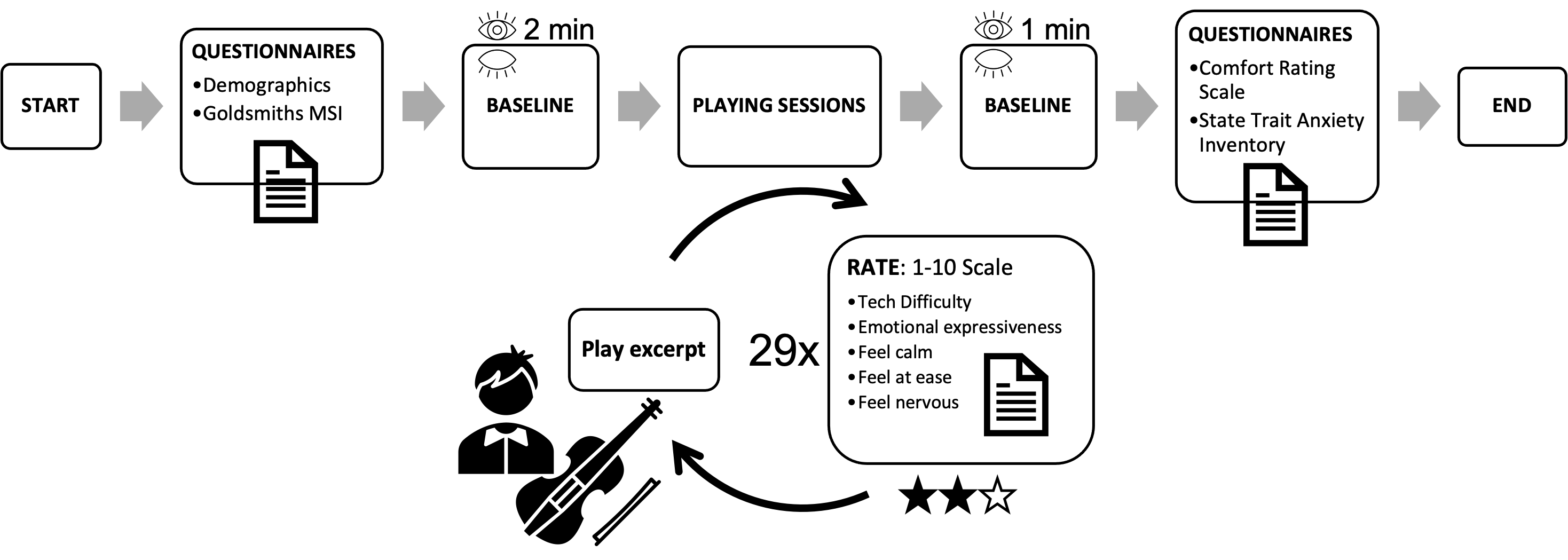
Figure 2. Experimental protocol

We pursued a two-staged Machine Learning (ML)model development approach. Our first stage comprises a gradual empirical development of an underlying behavioral model that serves as a basis for the capturing of the main target mental state of EML as a latent construct. Guided by the Challenges-$\&$-Skills view in the theory of flow, our experimental protocol was designed to modify the conditions necessary for the emergence of EML. As a concrete operationalization, we employed the task of violin playing with skilled musicians during practice sessions while manipulating the level of difficulty of the tasks. The behavioral model was rigorously built via inspection of the inter-construct relationships in the model and statistical assessment of their significance. Self-reported scales by the musicians during the experimental tasks were utilized as data input, complemented by synchronized sensor recordings. The results from the initial stage provided us with a dataset that incorporated time series sensor data along with validated labeling of EML.

In the second stage, we delved into the analysis of the captured dataset and enriched it with corresponding features. This was done for the elicitation of a near-real-time ML algorithm that relies solely on sensory input to determine the target condition of EML. This means using the raw labeled dataset, enriching it with corresponding features, and developing a machine-learning model to classify the perceived level of EML via sensor data as a sufficiently accurate surrogate for the paper-and-pencil scales that were employed in the first stage. This was followed by a meticulous evaluation of a few specific ML models, and the selection of the one that exhibited a favorable balance between accuracy and responsiveness, as assessed using conventional metrics. To address practical considerations, we additionally augmented this endeavor with sensor sensitivity analysis to ascertain the significance of individual sensor types in the predictive outcomes.

4. Stage I: The Experiment

The overall experimental process that was pursued is illustrated in Figure 2. Nine adult musicians (3 Males; 6 Females), with a mean age of 24 $\pm$ 2 years, and holding a conservatory degree in Violin, were randomly recruited and volunteered to participate in our study.

Ethical board approval was granted, and informed consent was obtained from all participants. As a first step, each participating violinist in the experiment was requested to complete a form containing general demographic information (e.g., gender, age, nationality). The questionnaire also included a section with the previously validated Goldsmiths Musical Sophistication Index (Gold-MSI)scale (Müllensiefen and et al., 2014). This scale consists of 39 questions designed to assess professional musical expertise across various dimensions of musicality. Particularly, the musician’s musical profile according to their Gold-MSI facet scores (average and percentile) catered: Active Engagement (47.14, 69), Perceptual Abilities (51.86, 55), Musical Training (41.14, 89), Emotions (33.29, 38), Singing Abilities (34.86, 61), and General Sophistication (96.86, 74). In comparison to the population norm, our subjects exhibited an average musical training level that ranked in the $89th$ percentile.

After filling out the questionnaires, the participants were equipped with a set of body-worn sensory devices, as illustrated in Figure 3. This included measurements of Electrocardiography (ECG), respiration rate, skin conductance (GSR), and motion tracking (IMU) of the wrist and the upper arm. The GSR Shimmer sensor was positioned on the index and middle finger of the bow-holding hand. Subsequently, a baseline measurement was taken in a relatively stationary standing position, capturing two minutes with eyes shut and two minutes with eyes open. These recordings were conducted to facilitate data normalization during the later analysis phase.

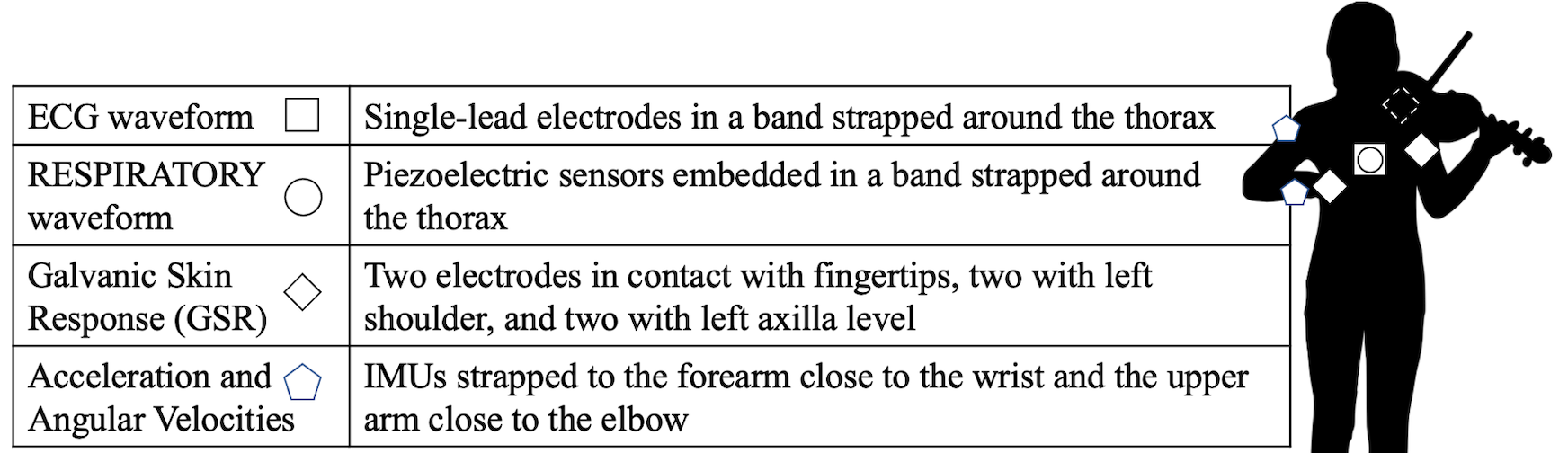
Figure 3. Wearable sensors

Following the baseline step, the main part of the experimental protocol was initiated. This consisted of repetitive playing sessions during which each violinist was instructed to play a series of 29 musical excerpts in a randomly assigned order. These excerpts constitute the total set manifested by a combination of excerpt category and tempo (Fernández-Sotos et al., 2016; Liu and et al., 2018) as further elaborated in Section 4.2.

After playing each individual excerpt, a questionnaire was administered to the violinists, asking them to rate their perceptions of the technical difficulty, emotional expressiveness, their level of calmness, ease, nervousness, and discomfort (Knight et al., 2002) resulting from wearing the sensors while playing the violin. All scales have been the basis for the behavioral model development in Section 4.2. The former two items have been part of the constructs that capture the intended manipulation of challenge complexity, and the latter were adopted from the scales that were administered at the end of the experiment.

Concluding the experimental protocol, each violinist repeated two 1-minute lasting baselines (with eyes open and eyes closed). Finally, once the sensor devices were removed, the violinist filled out two questionnaires, the Comfort Rating Scale (CRS) (Knight et al., 2002) and the State-Trait Anxiety Inventory (STAI) (Speilberger and et al., 1983) scale. The complete questionnaires can be found in the supplementary materials.

4.1. Data Description

The raw data consisted of two main datasets: $\mathcal{D}=\langle D_{qnr},D_{sns}\rangle$, where $D_{qnr}$ is a dataset consisting of all questionnaire responses, conforming to the tuple:

$$D_{qnr}=\langle K=(user_{id},trial_{index}\in(1...29),V\rangle,$$

in which each data row is identified by a unique compound key $K$ being the combination of the participant identifier and the trial index designating any one of the excerpts that were played, and $V$ is a union of all attributes with questionnaire ratings on a $1...10$ scale. This includes raw features unified also with an attribute for the computed factor of EML that was elicited as a latent construct as described in Section 4.2.

The second dataset $D_{sns}$ is a time-series dataset conforming to the tuple:

$$D_{sns}=\langle t,K=(user_{id},trial_{index}\in(1...29),S=(Sensor_{type},M)\rangle,$$

where $t$ is a timestamp of the measurement, $K$ is the key as in the first dataset, and $S$ is a sensor measurement denoting the type and its corresponding value. An exemplar dataset with data types, units, and descriptions is available at github.com/AnonymousAuthors.

4.2. Behavioral Model Development for Data Labeling

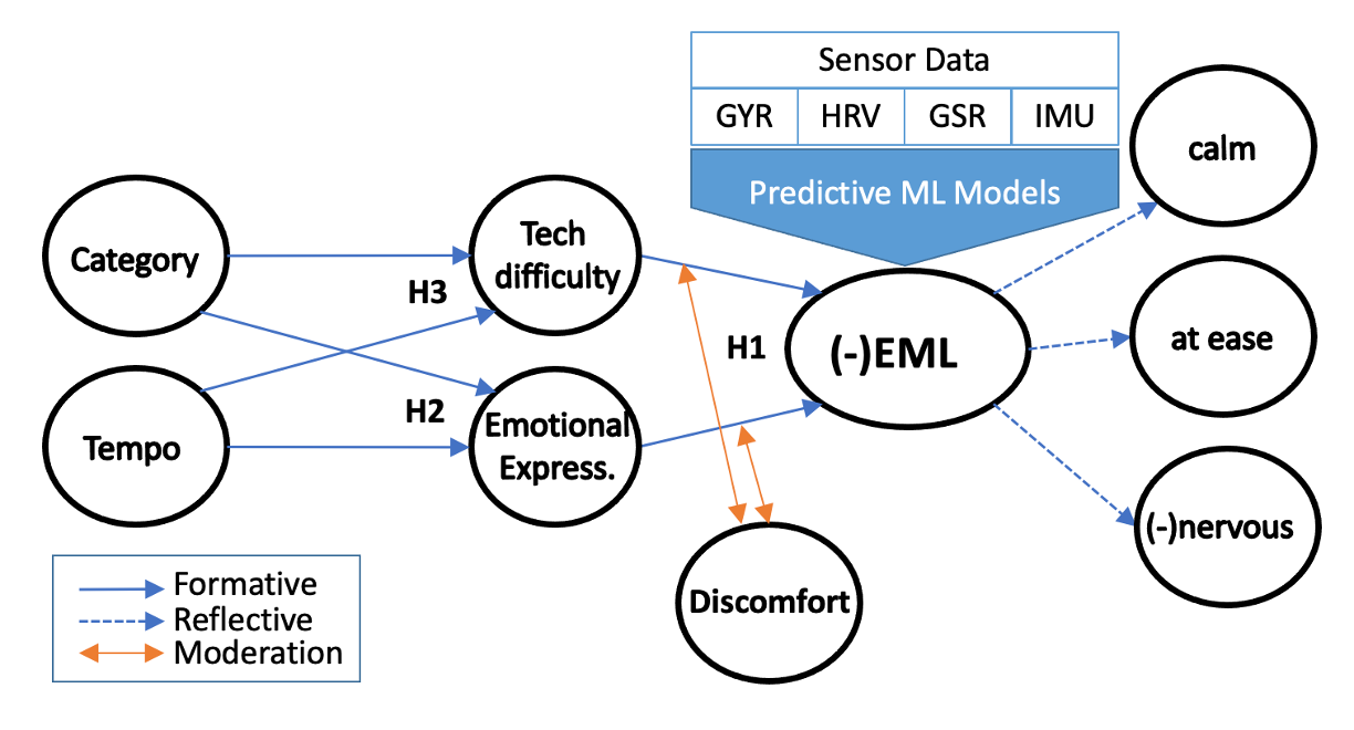
Figure 4. Behavioral-model for the manipulation of EML

We began the gradual development of the behavioral model illustrated in Figure 4. The objective was to establish a connection between the perceived manipulations of musical excerpts at different levels of technical difficulty and experienced emotional expressiveness, and the level of EML. The purpose of this model development was twofold: (1) to ensure that our experiment is effectively affecting the level of EML, and (2) to use the model for the labeling of our sensor-recordings with corresponding EML levels. We also wanted to take into consideration the possible perception of discomfort that may be associated with wearing the sensors while playing the violin. Hence, our main experimental hypothesis was:

Hypothesis 1 (H1).

Technical difficulty and emotional expressiveness for a played musical excerpt, as perceived surrogates of the manipulation, affect the learner’s engagement in the excerpt-playing task.

In order to effectively influence the perceptions of technical difficulty and emotional expressiveness, we employed a combination of two factors: excerpt tempo and type (i.e., musical category) as our direct stimuli. Overall, the collection of the excerpts assigned to each musician included excerpts of two types: 24 technical and 5 repertoire. For the technical type, the musicians were instructed to play 12 excerpts at a slow tempo, and 12 at a fast tempo (randomly ordered in the experimental protocol). For the repertoire type, musicians were instructed to play one at a fast tempo, two at an average tempo, and two at a slow tempo. This resulted in each musician playing a total of 29 sessions. As aforementioned, after each excerpt, the musician reported (on a 1–10 scale) their perceptions of technical-difficulty and of emotional-expressiveness. With respect to this setup, we hypothesized that:

Hypothesis 2 (H2).

Excerpt’s musical-category and played tempo affect learner’s perceived emotional-expressiveness.

Hypothesis 3 (H3).

Excerpt’s musical-category and played tempo affect learner’s perceived technical-difficulty.

The data collected in the questionnaires were examined to test for these two preceding desired effects. We conducted two-way ANOVA analyses to test for the possible effects in H2 and H3.

Table 1. Descriptive statistics for all measures

Measure	N	Min	Max	Mean	Std. Dev
tech_diff	261	1	10	4.12	2.405
emo_expr	261	1	10	4.36	2.699
feel_calm	261	1	10	7.03	2.089
feel_at_ease	261	1	10	7.11	2.041
feel_nervous	261	1	10	3.20	2.069
feel_uncomfortable	261	1	10	4.07	1.961

With respect to the effect on emotional-expressiveness (H2), the two-way interaction musical-category$*$tempo was not found to be significant, where only the main effect of musical-category was significant ($F_{(1,256)}=177.239$). There was no significant effect of the tempo at which the excerpt is played on emotional-expressiveness.

With respect to H3, both main effects of the category ($F_{(1,256)}=19.999$) and tempo ($F_{(2,256)}=50.611$) were found to be significant, but also was the two-way interaction between musical-category$*$tempo ($F_{1,256}=13.310$). Thus, post-hoc pair-wise comparisons indicated significant differences in the perception of technical-difficulty between the categories when the tempo is fast ($F_{1,115}=23.611$). The average tempo was considered only in the repertoire type. There was no significant difference in the perception of technical-difficulty between the categories when the tempo is slow.

Hence, the sole effect of the category manipulation is inconsistent across different levels of tempo, such that for a slow tempo, there is not much of a difference in the perception of technical-difficulty when the type of excerpt is altered. Therefore, it was essential to combine the manipulation of the excerpt-category jointly with the manipulation of tempo to ensure the perception of technical-difficulty is altered. Nevertheless, we concluded that our combined experimental stimuli were effective in altering both perceptions of technical-difficulty and emotional-expressiveness, allowing us to continue with the examination of the subsequent effect on EML as hypothesized in H1.

For labeling, we aimed to capture the extent to which each musician was immersed in the act of playing the excerpt. For this, we attended to the literature notion of being engaged in a task or being in a ‘flow’, as articulated by the Flow-Theory (Csikszentmihalyi, 1990). In line with this view, optimal EML is attained when in a proper balance between one’s level of personal competence and the perceived complexity level of the task at hand. As illustrated in Figure 1, the flow condition along the diagonal is reflected by a sweat-spot between anxiety and boredom. Particularly, the inclusion of more competent musicians in our experiment as corroborated by the Gold-MSI index, let us focus on the right-hand side of this chart, where EML may be conceived as balancing nervousness and relaxation along an increase in complexity of the task. To capture such a condition, after playing each excerpt, we employed self-reporting of calmness, being at ease, and nervousness perceptions using measures extracted from the STAI scale that was fully administered at the end of the experiment.

While EML is formed during the actual playing of a musical excerpt and manipulated via the aforementioned characteristics of the excerpts (i.e., technical-difficulty and emotional-expressiveness), the three measures of calmness, being at ease, and nervousness are expected to be mutually reflective (Freeze and Raschke, 2007) of the level of EML as a latent construct. These measurements require conventional validation through Cronbach’s Alpha (reliability) and Factor Analysis (convergence and discriminant validity). Respectively, reliability among the three measures was verified with Cronbach’s $\alpha=.922$. Principal component analysis was conducted, considering Eigenvalues greater than 1 (see Table 2). The minimum factor loading criterion was set to 0.50. The communality of the scale, indicating the amount of variance in each dimension, was also assessed to ensure acceptable levels of explanation. The results of this analysis confirmed a single component (namely EML) for all three measures. The factor loadings and communalities for the three factors, feel_calm, feel_at_ease, and inv_nervous, are (0.972, 0.945), (0.931, 0.867), and (0.784, 0.614), respectively.

Table 2. Factor Analysis:
feel_calm, inv_nervous, feel_at_ease $\xrightarrow{}$ nirvana

Total Variance Explained
	Initial Eigenvalues			Sums of Squared Loadings
Factor	Total	% of Variance	Cumulative %	Total	% of Variance
1	2.600	86.662	86.662	2.425	80.843
2	0.307	10.234	96.896
3	0.093	3.104	100.000

Following dimensionality reduction for EML as the latent construct, we then moved on to testing our main hypothesis (i.e., H1). Additionally, we took into consideration the potential effect of perceived discomfort associated with wearing additional sensors while playing the violin. Therefore, we speculated that the perception of discomfort might moderate the hypothesized main effects (i.e., a high sense of discomfort could potentially hinder the experienced EML). To explore this, we conducted a two-way ANCOVA analysis for H1, with discomfort included as a covariate. The results, as presented in Table 3, indicate significant main effects on EML for both technical-difficulty ($F_{(9,185)}=6.492,p<.001$) and emotional-expressiveness ($F_{(9,185)}=50.584,p=.002$). Moreover, the covariate, discomfort was found to be significantly associated with EML ($F_{(1,185)}=7.59,p=.006$).

Table 3. Ancova for H1: tech_diff, emot_expr (independent), discomfort (covariant) $->$ EML

Tests of Between-Subjects Effects
Source	Type 3 SSE	df	Mean Square	F	Sig.
Corrected Model	4171.661a	75	55.622	3.379	$<$0.001
Intercept	8210.182	1	8210.182	498.697	$<$0.001
feel_uncomfortable	124.962	1	124.962	7.590	0.006
emo_expr	455.260	9	50.584	3.073	0.002
tech_diff	961.923	9	106.880	6.492	$<$0.001
emo_expr * tech_diff	1269.709	56	22.673	1.377	0.059
Error	3045.704	185	16.463
Total	102481.211	261
Corrected Total	7217.365	260

The effect size of the statistical analyses is as follows: Technical difficulty 13.3%, Emotional expressiveness 6.3%, Discomfort 1.7%, Interaction (tech * emotional exp) 17.5% (not significant), Error 42.1%, and total for model ($R^{2}$) 57.8%.

Concluding the effort in developing the behavioral model, we have successfully created and validated the necessary instrumentation for manipulating and measuring EML through self-reporting. We have also identified that the perception of discomfort may have a moderating effect on EML. Hence, we used the developed model to label the sensor dataset, where we partitioned between ‘high’ and ‘low’ EML as was naturally split by its mean value. Additionally, we utilized the reporting of discomfort as another target label. This was done to allow for the development of two ML models with the acquired sensor data: (1) discomfort prediction, and (2) classification of EML. The output from model (1) was used as an additional input feature for model (2) due to its significant moderating effect.

5. Stage II: Machine learning model development

The primary objective of this stage was to develop a ML model that can classify a musician’s EML while playing the violin, utilizing the sensor data that were labeled in the previous stage.

5.1. Data preparation for ML

We established two parameters, namely step-size and window-size, and employed them to partition each excerpt’s sensor dataset into windows. For example, if the step-size is set to $20$ seconds and the window-size is set to $30$ seconds, the dataset for each excerpt is divided into a sequence of $30$-second windows with a $10$-second overlap between any two adjacent windows. The motivation for such windowing is two-fold. Firstly, it allows us to be more responsive in terms of the time required for making a prediction. If we do not partition the excerpt, predictions can only be made per expert, which occurs approximately every $90$ seconds on average. Secondly, for the application of machine learning algorithms, a sufficient sample size is needed ($261$ data points without windowing). The concrete determination of these parameters is discussed in Section 6.

A total of $257$ features were computed from the sensor data for each window. We used out-of-box sensor libraries such as PyEDA and PyHRV to extract the features. The sensor data were enriched with a first derivative termed “jerk”, defined as the difference in values divided by the difference in time between two adjacent entries. It was computed for the IMU and GYR data. In addition, the magnitude of the 3-axis sensors was determined by taking the square root of the sum of squares of the sensor values. The magnitude calculation was performed for both the IMU and GYR data, along with their respective jerk values, across the x, y, and z axes.

From the IMU and GSR sensors, we extracted several features including the interquartile ratio, kurtosis, mean, median, RMSSD (the root-mean-square of differences between successive RR intervals), skewness, and variance of both magnitude and jerk-magnitude. Specifically, from the IMU sensor, we also extracted the SPARC index (Balasubramanian et al., 2012) as a feature, which denotes the smoothness of movement associated with the IMU positioned on the forearm. From the HRV sensor, we extracted various features including the mean, median, frequency domain features (e.g., LF, HF, VLF), time domain features (e.g., RMSSD, NNI@20, NNI@50, PNNI@20, PNNI@50, NNI range, SDNN), as well as non-linear measures (e.g., SampEntropy, SD1, SD1/SD2). From the GSR sensors, features were extracted with the PyEDA library, catering to a combination of statistical features such as the number of peaks, amplitude mean, variance, and automatic features using autoencoding.

Prior to feature extraction, we investigated the correspondence between the GSR and IMU sensors, to accommodate for any undesired movement artifacts (Society for Psychophysiological Research Ad Hoc Committee on Electrodermal Measures, 2012) that could interfere with the accuracy of the GSR sensor readings. Specifically, we performed a Pearson correlation test to examine the correlation between the readings of each individual GSR sensor and the IMU. The results indicated that both correlations were insignificant. Therefore, there was no need to discard any of the GSR measurements, as they were not affected by the movement artifacts captured by the IMU sensor.

Post-feature extraction, we used the eye-closed task (baseline sessions) for inter-subject normalization to account for the individual differences among participants. For each $\langle$user X feature$\rangle$ in the baseline trials, a corresponding mean value was calculated. Subsequently, each feature of the non-baseline excerpts was divided by the corresponding baseline mean value of that feature.

Each window was labeled with the EML level (‘high’ or ‘low’) and discomfort level, both based on the scores determined by the mental model that was developed in the previous stage. It is important to note that the original data labels were determined at the level of each excerpt as a whole, based on the original musician’s indications reported at the end of each excerpt. We then interpolated each value across all windows that correspond to the same excerpt. This hints at an assumption that the user’s EML and sense of discomfort are two relatively stable conditions that do not undergo significant changes during the course of playing an individual excerpt.

5.2. Predicting the discomfort level

During the development of the mental model, we observed that the discomfort level is a covariant with respect to the EML. We thus presume that an EML classification model may benefit if it also utilizes the discomfort level as an input. This has required us to develop a designated model for the prediction of discomfort with sensor data as an input (see Figure 6).

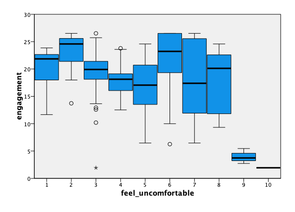
Figure 5. Box-plot of EML (‘engagement’) levels for each discomfort level

As an initial step, we examined the relationship between feeling discomfort and EML using box-plot distributions, as shown in Figure 5. This chart highlighted the most profound difference between the discomfort segments of $[1-8]$ and $[9-10]$, with EML dropping significantly in the latter. Accordingly, we split the data into bins labeled ‘high discomfort’ and ‘normal discomfort’.

Utilizing the discomfort labeling, we trained a binary classification model that takes the sensor data as input and predicts whether the discomfort level is ‘normal’ or ‘high’. We performed a $5$-fold cross-validation (Kohavi et al., 1995). An average accuracy level of $0.98$ was achieved with an SVM classifier without hyperparameter optimization. The two most important features for classification were found to be the variance of the IMU and the variance of the GYR.

This suggests that we can easily track the discomfort level with the sensors, and we do not need a sophisticated ML model to do so. This should not come as a surprise, as the discomfort level is highly correlated to the variance of the GYR sensor.

Figure 6. ML engagement prediction pipeline

6. Results

We partitioned the data randomly into five parts. Each part served as a test set once, while the other four parts were used for training (i.e., 5-fold cross-validation with $20\%$ for testing and $80\%$ for training (Kohavi et al., 1995)). The partitioning was carefully designed to prevent data leakage between training and test sets. That is, during the preparation of the data for the five-fold cross-validation, we ensured that data from the same parts of the excerpts did not exist in both the training and testing set.

We report the average results for a fixed $30$-second window-size with the top-performing XGBoost algorithm in Figure 7. Both $F_{1}$ and $accuracy$ scores were observed. The class balance was $54\%$ for ‘low’ EML and $46\%$ for ‘high’ EML.

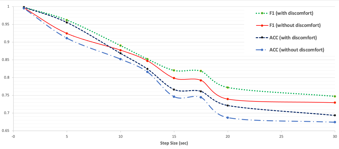
Figure 7. $F_{1}$ and $ACC$ scores with $5$-fold cross validation for different step-size values; with window-size of $30$ seconds.

We conducted a sensitivity check for both the window size and the step size using the top-performing XGBoost algorithm. Regarding the window size, we followed the convention suggested in (Zeltyn et al., 2016) for general activity recognition and set it to a fixed duration of $30$ seconds. Modifying it only had a marginal impact on the results. Therefore, a window size of $30$ seconds was chosen as a sweet spot. This duration was long enough to provide sufficient informative sensor data for model training, yet short enough to maintain model responsiveness by generating predictions every few seconds.

With respect to the manipulation of step size, as illustrated in Figure 7, we decided to set it at $15$ seconds. This means that the model would provide an initial output after 30 seconds and subsequent predictions every 15 seconds. The overlapping windows ensured a degree of statefulness in the evolution of EML. We recognized the potential of using a model like LSTM, which inherently has a ’memory’ component in its architecture. We interpreted the increase in accuracy for a shorter step-size (below the bending point at 15 seconds) as mainly stemming from a synthetic improvement resulting from extensive window overlapping, where more than half of a window overlaps with the adjacent windows. We also tested with different step sizes (e.g., 30) and observed that most results remained consistent.

For the construction of the main ML model for EML, we resorted to a commercial AI service, which had a variety of models available. The key models we experimented with included Decision Tree, Gradient Boosting, LGBM, Logistic Regression, Random Forest, SVM Classifier, and XGBoost. We opted to use the default hyperparameters for all of these algorithms. Although the commercial tool offered automatic hyperparameter optimization, the resulting improvements were found to be insignificant.

The top-performing result was achieved by the XGBoost classifier, which obtained an $F_{1}$ score of $0.82$ when the discomfort feature was included in its input. When the discomfort level was ignored, the performance of the models decreased by approximately 5%. We also conducted tests comparing the XGBoost classifier with other algorithms. We employed a non-parametric bootstrapping test (Efron and Tibshirani, 1994; Dror et al., 2019) and used 5-fold cross-validation for the evaluation of the results. The XGBoost classifier demonstrated a significant improvement ($p<0.01$) compared to the other algorithms when the step-size was larger than $10$. As shown in Table 4, the classifier demonstrates good results for both the “low” and “high” engagement classes.

Table 4. A confusion matrix for one of the 5-fold validation.

	Predicted EML
Observed EML	‘high’	‘low’	Percent correct
‘high’	41	8	83.7%
‘low’	7	62	89.9%
Percent correct	85.4%	88.6%	87.3%

In addition to the XGBoost classifier, the three top-performing algorithms were the LGBM classifier, the Decision Tree Classifier, and logistic regression. Table 5 presents the feature importance for these different algorithms. For tree-based classification algorithms like Decision Tree, XGBoost, and LGBM, the feature importance represents their inherent importance scores, calculated based on the reduction in the criterion used to select split points during training. For non-tree algorithms such as Logistic Regression, the feature importance reflects the importance determined by training a Random Forest algorithm on the same training data as the non-tree algorithm. For each sensor type, the most important feature is displayed.

Table 5. Feature importance.

	IMU	GYR	GSR	HRV
XGBoost	elbow_jerk_var	elbow_rmssd	left_axilla	high_frequency
LGBM	elbow_kurt	wrist_jerk_kurt	left_axilla	mean_nni
Decision Tree	wrist_magnitude_rmssd	elbow_jerk_median	left_axilla	high_frequency
Logistic Regression	wrist_magnitude_rmssd	elbow_jerk_median	left_axilla	high_frequency

Table 6. $F_{1}$ scores of the different algorithms with the different sensors.

	IMU	GYR	GSR	HRV	IMU +GYR	GSR +HRV	ALL
XGBoost	0.779	0.751	0.723	0.741	0.812	0.748	0.820
LGBM	0.773	0.716	0.707	0.585	0.808	0.718	0.811
Decision Tree	0.707	0.726	0.698	0.686	0.741	0.703	0.771
Logistic Regression	0.693	0.704	0.708	0.578	0.723	0.717	0.753

Note that the GSR sensors were placed in three positions: left shoulder, right-hand fingertips, and left axilla. As shown, the GSR feature from the left axilla location is the most indicative. Additionally, the IMU and GYR sensors were placed on the wrist and elbow, and the data were enriched with a first derivative (“jerk”). Table 5 suggests that the “jerk” feature plays a significant role as an input for almost all algorithms. For the HRV class, the high frequency (HF) feature is the most influential in most algorithms.

Table 6 concludes our model development results, presenting a comparison of the accuracy achieved by the four algorithms. The columns represent different sensor subsets that were used as input for the classification algorithm. As observed, the combination of the IMU sensors and GYR sensors yields an average approximation of $97\%$ for the optimal $F_{1}$ score (with all features), while GSR and HRV achieve an average of $91\%$ of the total $F_{1}$ score. Furthermore, the feature extraction for GSR is based on an auto-encoder algorithm, which results in a relatively high time complexity. This suggests that we can potentially reduce the number of calculated features or sensors without significantly compromising accuracy, while significantly improving the time complexity.

According to the Flow theory, the relatively good model achieved by the motion components (i.e., IMU + GYR) can be attributed to the distinctive nature of motor activities. Considering the inclusion of highly trained musicians, EML is experienced only when the task complexity is high, which is likely to be reflected in high motion volatility.

For replicability of our results, a lightweight version of the trained XGBoost model ($F_{1}=0.801$) is available at github.com/AnonymousAuthors We have also included an XGBoost wrapper that allows users to experiment with model training using their own datasets.

7. Conclusion and Future work

Our work presents a model for the continuous classification of EML. We employed an experimental environment with skilled participants who played the Violin while sensor data were collected. To employ supervised learning, we annotated the data by developing a behavioral model. Subsequently, we increased the data density by utilizing interpolation. The labels served as an input for training a machine learning model that predicts the musician’s EML in near real-time. We discussed in detail the data preparation methodology for the machine learning model, analyzed the results, and performed a sensitivity analysis with respect to the different sensor types.

We acknowledge that our model may still be susceptible to further testing of its performance in other realistic settings. As a first step in this direction, we applied our model to the recordings in our experiment to produce a prototypical engagement footprint for each excerpt. Our aim is to employ a panel of experienced musicians to validate its faithfulness to the actual musical temperament of each excerpt.

We also note that our setup excluded a leave-1-user-out configuration since we assumed that, in learning contexts such as in our case (i.e., violin practice sessions), it is plausible to capture a baseline recording from each user. However, in the future, we may relax this assumption and attempt a more generalizable configuration.

In the future, we intend to deploy the developed model into a broader teacher-learner interaction system. This system will enable the ongoing tracking of EML as part of the information about the learner’s state. It will be particularly useful as learners gradually improve and progress along the motor learning activity. The measurement of EML will serve as a key feedback mechanism for the instructor, who has control over the learning pace and rewards allotted to the student’s performance.

Furthermore, our future plans include employing the instrumentation for other motor learning activities, such as handwriting and drum playing in children. This will provide an opportunity to test the applicability of the developed instrumentation with different types of motor learning activities, ensuring its robustness.

Appendix A Appendix

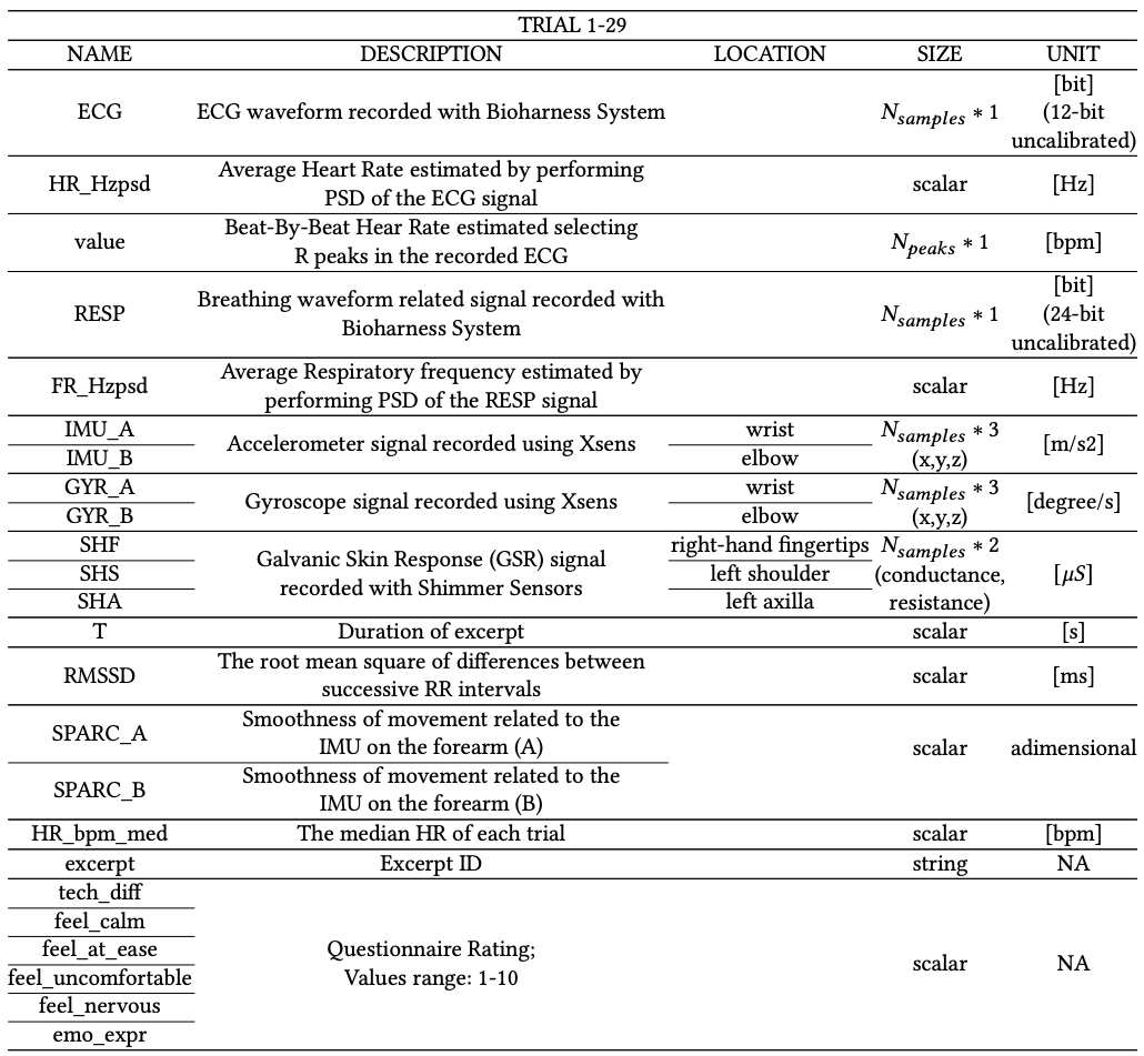
Figure 8. Experimental measurements

References

- (1)
- Aslan and et al. (2014) Sinem Aslan and et al. 2014. Learner Engagement Measurement and Classification in 1:1 Learning. In 2014 13th International Conference on Machine Learning and Applications. , , 545–552.
- Balasubramanian et al. (2012) Sivakumar Balasubramanian, Alejandro Melendez-Calderon, and Etienne Burdet. 2012. A Robust and Sensitive Metric for Quantifying Movement Smoothness. IEEE Transactions on Biomedical Engineering 59, 8 (2012), 2126–2136.
- Basdogan et al. (2000) Cagatay Basdogan, Chih-Hao Ho, Mandayam A. Srinivasan, and Mel Slater. 2000. An Experimental Study on the Role of Touch in Shared Virtual Environments. ACM Trans. Comput.-Hum. Interact. 7, 4 (dec 2000), 443–460.
- Berka and et al. (2007) Chris Berka and et al. 2007. EEG correlates of task engagement and mental workload in vigilance, learning, and memory tasks. Aviation, space, and environmental medicine 78 (06 2007), B231–44.
- Bower (1992) Gordon H Bower. 1992. How might emotions affect learning. The handbook of emotion and memory: Research and theory 3 (1992), 31.
- Bulger and et al. (2008) Monica Bulger and et al. 2008. Measuring Learner Engagement in Computer-Equipped College Classrooms. Journal of Educational Multimedia and Hypermedia 17 (04 2008).
- Csikszentmihalyi (1990) Mihaly Csikszentmihalyi. 1990. Flow: The psychology of optimal experience. Vol. 1990. Harper & Row, New York.
- Csikszentmihalyi (2000) Mihaly Csikszentmihalyi. 2000. Beyond boredom and anxiety. Jossey-bass, 25th Anniversary edition.
- Csikszentmihalyi and Csikszentmihalyi (1988) Mihaly Csikszentmihalyi and Isabella Selega Csikszentmihalyi. 1988. Optimal experience: Psychological studies of flow in consciousness. Cambridge university press, UK.
- DiSalvo et al. (2022) Betsy DiSalvo, Dheeraj Bandaru, Qiaosi Wang, Hong Li, and Thomas Plötz. 2022. Reading the Room: Automated, Momentary Assessment of Student Engagement in the Classroom: Are We There Yet? Proc. ACM Interact. Mob. Wearable Ubiquitous Technol. 6, 3, Article 112 (sep 2022), 26 pages.
- Dror et al. (2019) Rotem Dror, Segev Shlomov, and Roi Reichart. 2019. Deep Dominance - How to Properly Compare Deep Neural Models. In Proceedings of the 57th Annual Meeting of the Association for Computational Linguistics. Association for Computational Linguistics, Florence, Italy, 2773–2785.
- Dubovi (2022) Ilana Dubovi. 2022. Cognitive and emotional engagement while learning with VR: The perspective of multimodal methodology. Computers & Education 183 (2022), 104495.
- Efron and Tibshirani (1994) Bradley Efron and Robert J Tibshirani. 1994. An introduction to the bootstrap. CRC press, USA.
- Fairclough and et al. (2009) Stephen H Fairclough and et al. 2009. Measuring task engagement as an input to physiological computing. In 2009 3rd International Conference on Affective Computing and Intelligent Interaction and Workshops. IEEE Computer Society, Los Alamitos, CA, USA, 1–9.
- Fernández-Sotos et al. (2016) Alicia Fernández-Sotos, Antonio Fernández-Caballero, and José M Latorre. 2016. Influence of tempo and rhythmic unit in musical emotion regulation. Frontiers in computational neuroscience 10 (2016), 80.
- Freeze and Raschke (2007) Ronald D. Freeze and Robyn L. Raschke. 2007. An Assessment of Formative and Reflective Constructs in IS Research. In ECIS. University of St. Gallen, St. Gallen, Switzerland, 171.
- Ganesh and et al. (2014) Gowrishankar Ganesh and et al. 2014. Two is better than one: Physical interactions improve motor performance in humans. Scientific reports 4, 1 (2014), 1–7.
- Gao et al. (2022) Nan Gao, Mohammad Saiedur Rahaman, Wei Shao, Kaixin Ji, and Flora D. Salim. 2022. Individual and Group-Wise Classroom Seating Experience: Effects on Student Engagement in Different Courses. Proc. ACM Interact. Mob. Wearable Ubiquitous Technol. 6, 3, Article 115 (sep 2022), 23 pages.
- Gorman and et al. (2004) Jack M Gorman and et al. 2004. The effect of successful treatment on the emotional and physiological response to carbon dioxide inhalation in patients with panic disorder. Biological Psychiatry 56, 11 (2004), 862–867.
- Katsis et al. (2011) Christos D Katsis, Nikolaos S Katertsidis, and Dimitrios I Fotiadis. 2011. An integrated system based on physiological signals for the assessment of affective states in patients with anxiety disorders. Biomedical Signal Processing and Control 6, 3 (2011), 261–268.
- Knight et al. (2002) James F Knight, Chris Baber, Anthony Schwirtz, and Huw William Bristow. 2002. The Comfort Assessment of Wearable Computers.. In iswc, Vol. 2. Citeseer, IEEE, Seattle, Washington, 65–74.
- Kohavi et al. (1995) Ron Kohavi et al. 1995. A study of cross-validation and bootstrap for accuracy estimation and model selection. In Ijcai, Vol. 2. Montreal, Canada, Morgan Kaufmann Publishers Inc., San Francisco, CA, USA, 1137–1145.
- Lanata et al. (2012) Antonio Lanata, Gaetano Valenza, and Enzo Pasquale Scilingo. 2012. A novel EDA glove based on textile-integrated electrodes for affective computing. Medical & biological engineering & computing 50, 11 (2012), 1163–1172.
- Lee et al. (2019) Victor R. Lee, Liam Fischback, and Ryan Cain. 2019. A wearables-based approach to detect and identify momentary engagement in afterschool Makerspace programs. Contemporary Educational Psychology 59 (2019), 101789.
- Li (2021) Shan Li. 2021. Measuring Cognitive Engagement: An Overview of Measurement Instruments and Techniques. International Journal of Psychology and Educational Studies 8 (07 2021), 63–76.
- Liu and et al. (2018) Ying Liu and et al. 2018. Effects of musical tempo on musicians’ and non-musicians’ emotional experience when listening to music. Frontiers in Psychology 9 (2018), 2118.
- Martocchio (1994) Joseph J Martocchio. 1994. Effects of conceptions of ability on anxiety, self-efficacy, and learning in training. Journal of applied psychology 79, 6 (1994), 819.
- Müllensiefen and et al. (2014) D Müllensiefen and et al. 2014. Measuring the facets of musicality: The Goldsmiths Musical Sophistication Index. Personality and Individual Differences 60 (2014), S35.
- Provenzale and et al. (2021) Cecilia Provenzale and et al. 2021. Assessing the Bowing Technique in Violin Beginners Using MIMU and Optical Proximity Sensors: A Feasibility Study. Sensors 21, 17 (2021), 1–14.
- Rajendra Acharya and et al. (2006) U Rajendra Acharya and et al. 2006. Heart rate variability: a review. Medical and biological engineering and computing 44, 12 (2006), 1031–1051.
- Reed and Peshkin (2008) Kyle B. Reed and Michael A. Peshkin. 2008. Physical Collaboration of Human-Human and Human-Robot Teams. IEEE Transactions on Haptics 1, 2 (2008), 108–120.
- Santhalingam et al. (2023) Panneer Selvam Santhalingam, Parth Pathak, Huzefa Rangwala, and Jana Kosecka. 2023. Synthetic Smartwatch IMU Data Generation from In-the-Wild ASL Videos. Proc. ACM Interact. Mob. Wearable Ubiquitous Technol. 7, 2, Article 74 (jun 2023), 34 pages.
- Shaffer and Ginsberg (2017) Fred Shaffer and Jay P Ginsberg. 2017. An overview of heart rate variability metrics and norms. Frontiers in public health 5 (2017), 258.
- Society for Psychophysiological Research Ad Hoc Committee on Electrodermal Measures (2012) Society for Psychophysiological Research Ad Hoc Committee on Electrodermal Measures. 2012. Publication recommendations for electrodermal measurements. Psychophysiology 49, 8 (2012), 1017–1034.
- Speilberger and et al. (1983) CD Speilberger and et al. 1983. Manual for the Stait-Trait Anxiety Inventory, 1983.
- Valenza and et al. (2014) Gaetano Valenza and et al. 2014. Revealing real-time emotional responses: a personalized assessment based on heartbeat dynamics. Scientific reports 4, 1 (2014), 1–13.
- Warr and Bunce (1995) Peter Warr and David Bunce. 1995. Trainee characteristics and the outcomes of open learning. Personnel psychology 48, 2 (1995), 347–375.
- Wu et al. (2012) Chi-Keng Wu, Pau-Choo Chung, and Chi-Jen Wang. 2012. Representative segment-based emotion analysis and classification with automatic respiration signal segmentation. IEEE Transactions on Affective Computing 3, 4 (2012), 482–495.
- Zeltyn et al. (2016) Sergey Zeltyn, Lior Limonad, and Alexander Zadorojniy. 2016. Enhanced sliding window approach for the inertial-based activity recognition. In Proceedings of the 1st joint workshop on Smart Connected and Wearable Things 2016. TUprints, Darmstadt, 20.