Atoms in a spin-dependent optical lattice potential as a topological insulator with broken time-reversal symmetry

Abstract

We investigate fermionic ⁶Li $F=1/2$ atoms in a 2D spin-dependent optical lattice potential (SDOLP) generated by intersecting laser beams with a superposition of polarizations. The effective interaction of a Li atom with the electromagnetic field contains a scalar and vector (called as fictitious magnetic field, ${\bf B}_{\mathrm{fic}}$) contribution. We calculate the band structure of Li atoms in the SDOLP as a function of the laser intensity and an external magnetic field ${\bf B}_{\mathrm{ext}}=B_{\mathrm{ext}}{\hat{\bf z}}$. We also calculate the Chern numbers of the SDOLP and show that depending on $B_{\mathrm{ext}}$, the system is an ordinary insulator, an Abeliean topological insulator (TI), or a non-Abelian TI. Introducing a blue-detuned laser potential, $V_{\mathrm{BD}}(y)=V_{\mathrm{BD},0}(y)\Theta(|y|-L_{y}/2)$, results in edges for the SDOL. We calculate the resulting edge states (some of which are topological) and study their density, current density, spin-current density and correlate the edge states with the Chern numbers.

Introduction: A topological insulator (TI) is a material whose interior cannot conduct an electric current while its surface (edges) supports such a flow, i.e. the surface is an electric conductor [1, 3, 2, 4, 5]. A TI differs from an ordinary insulator in that it is not possible to continuously deform spin-orbit-induced topological insulators into an ordinary one without closing the bulk gap, i.e., without realizing the topological phase transition, and the presence of time-reversal symmetry is crucial for that [6]. TIs have been theoretically studied [3, 1, 7] and experimentally realized in a variety of systems, including HgTe/CdTe semiconductor quantum wells [8], BiSb alloys [9], and Bi₂Se₃ crystals [10, 11].

Recently there has been significant progress in realizing band structures with nontrivial topology in experiments with cold atomic gases [4, 5]. An advantage in using cold atoms in studying topological phases of matter is that their experimental parameters can be very well controlled. Nevertheless, significant challenges remain in developing techniques to generate fictitious magnetic fields and spin-orbit coupling for neutral atoms (for a recent advances in the field see Refs. [4, 12, 13, 14]). Another attempt to overcome technical difficulties is to put atoms in a 2D spin-dependent optical lattice potential (SDOLP). A recent study of fermionic and bosonic atoms in SDOLP in the limit of singly occupied sites was carried out in Refs. [15, 16]. In addition to determining the wave functions and energy levels of the atoms in the SDOLP, it was shown that such systems could be used as high precision rotation sensors, accelerometers, and magnetometers.

In this Letter we consider a cold fermionic gas of ⁶Li $F=1/2$ atoms in a SDOLP and an external magnetic field. We show that the properties of the system are significantly enriched relative to the system without external magnetic field, and that a radical change of the topological properties can be observed as the strength of the external magnetic field is varied. We calculate the band-structure and the Chern numbers (the topological invariants that classify bands in topological materials [1, 3, 2, 5, 4]) of the bands. Then, we apply blue-detuned lasers which introduce edges to the SDOL. The topological edge states (TES) close the gaps between bands and determine the character of topological phases. Both Abelian and non-Abelian TI phases are found, and simultaneous atomic and spin currents of the TES exist.

SDOLP: The atom Hamiltonian in the SDOLP is

$$H=-\frac{\hbar^{2}}{2M}\,\nabla^{2}+H_{\mathrm{Stark}}({\bf r})+H_{Z}.$$ (1)

The first term on the right hand side of Eq. (1) is the kinetic energy operator of an atom, where $M$ is the atomic mass. The last term on the right hand side of Eq. (1), $H_{Z}=-g_{F}\mu_{B}\,B_{\mathrm{ext}}F_{z}$, is the Zeeman interaction Hamiltonian of the atom with an external magnetic field ${\bf B}_{\mathrm{ext}}=B_{\mathrm{ext}}{\hat{\bf z}}$. The middle term, $H_{\mathrm{Stark}}({\bf r})$, is the optical lattice Stark interaction Hamiltonian. It is calculated as a second-order ac Stark shift [17] created by four laser beams that are tightly focused in the $z$ direction, and produce a 2D SDOLP, similar to the SDOLP in Ref. [15]. The complex slowly varying envelope ${\bf E}({\bf r})$ of the electric field ${\bm{\mathcal{E}}}({\bf r},t)=({\bf E}({\bf r})e^{-i\omega_{l}t}+{\rm{c.c.}})/2$ is given by ${\bf E}({\bf r})=\tfrac{E_{0}}{\sqrt{2}}\sum_{n=1}^{4}\left({\hat{\bf z}}+{\hat{\bf k}}_{n}\times{\hat{\bf z}}\right)e^{i{\bf k}_{n}\cdot{\bf r}}$, where ${\bf r}=(x,y)$, ${\hat{\bf z}}$ is the polarization unit vector along the $z$-axis, the wavevectors are ${\bf k}_{n}=k_{l}\,(\cos[(2n+1)\pi/4],\,\sin[(2n+1)\pi/4],\,0)$, $k_{l}=2\pi/\lambda_{l}$ is the laser wavenumber, $\lambda_{l}$ is the laser wavelength, and ${\hat{\bf k}}_{n}$ is the unit vector in the direction of ${\bf k}_{n}$. For ⁶Li, the total electronic angular momentum is $J=1/2$, hence, the effective interaction of an atom with the electromagnetic field can be described using a scalar potential $V$ and vector potential containing what Cohen-Tannoudji and Dupont-Roc called the fictitious magnetic field ${\bf B}_{\mathrm{fic}}$ [15, 17, 18, 19], and the tensor terms vanish: $H_{\mathrm{Stark}}({\bf r})=V({\bf r})-g_{F}\mu_{B}{\bf B}_{\mathrm{fic}}({\bf r})\cdot{\bf F}.$ Here ${\bf F}$ is the atomic hyperfine angular momentum, $\mu_{B}$ is the Bohr magneton, and for a ground state alkali atom with $L=0$, $J=S=1/2$, $I=1$ nuclear spin, $g_{F}=g_{S}\,\tfrac{F(F+1)-I(I+1)+S(S+1)}{2F(F+1)}$, and $g_{S}$ is the electron spin $g$-factor. The SDOLP is given by $V({\bf r})=-\tfrac{\alpha_{0}(\omega_{l})}{4}{\bf E}^{*}({\bf r})\cdot{\bf E}({\bf r})$ and ${\bf B}_{\mathrm{fic}}({\bf r})=\tfrac{i}{g_{F}\mu_{B}}\,\tfrac{\alpha_{1}(\omega_{l})}{4(2I+1)}\,{\bf E}^{*}({\bf r})\times{\bf E}({\bf r})$. Explicitly,

$$V({\bf r}) = -\frac{V_{0}}{2}\,\Big{[}2+\cos\big{(}q_{0}x\big{)}+\cos\big{(}q_{0}y\big{)}\Big{]},$$ (2)

$${\bf B}_{\mathrm{fic}}({\bf r}) = -B_{0}{\hat{\bf x}}\,\sin\big{(}q_{0}x\big{)}\,\cos^{2}\Big{(}\frac{q_{0}y}{2}\Big{)}$$ (3)

$$-B_{0}{\hat{\bf y}}\,\sin\big{(}q_{0}y\big{)}\,\cos^{2}\Big{(}\frac{q_{0}x}{2}\Big{)}.$$

Here $\alpha_{0}$ and $\alpha_{1}$ are scalar and vector polarizabilities which depend upon the detunings of the laser frequency $\omega_{l}$ from the D₁ and D₂ resonance lines of Li, $V_{0}=\alpha_{0}E_{0}^{2}$, $B_{0}=\tfrac{\sqrt{2}}{(2I+1)g_{F}\mu_{B}}\alpha_{1}E_{0}^{2}$ and $q_{0}=k_{l}/\sqrt{2}$. We use a laser frequency $\omega_{l}$ which is red-detuned from the Li D₂ line by $\Delta=-2\pi\times$642.6 MHz. In the current study we focus on band structure and assume that atomic wave functions need not be well localized within a Wigner-Seitz cell. Note that the divergence of the fictitious magnetic field does not vanish; ${\bf B}_{\mathrm{fic}}({\bf r})$ corresponds to a radially distributed magnetic monopole density. The Hamiltonian (1) has square lattice symmetry with lattice vectors ${\bf a}_{1}=(a_{0},0)$ and ${\bf a}_{2}=(0,a_{0})$, where the lattice period is $a_{0}=2\pi/q_{0}$, hence the reciprocal lattice has square symmetry with reciprocal lattice vectors ${\bf q}_{1}=(q_{0},0)$ and ${\bf q}_{2}=(0,q_{0})$.

The quantum states of the atoms in the SDOLP are parametrized by wavevector ${\bf k}=(k_{x},k_{y})$ belonging to the first Brillouin zone (BZ) of the SDOLP: $|k_{x},k_{y}|<q_{0}/2$, and the energy band number $n$, where $n$ is a positive integer. The corresponding energies $\epsilon_{n,{\bf k}}$ and wave functions $\psi_{n,{\bf k}}({\bf r})$ are determined from the Schödinger equation $H\psi_{n,{\bf k}}({\bf r})=\epsilon_{n,{\bf k}}\psi_{n,{\bf k}}({\bf r})$. The Schödinger equation was solved numerically using Mathematica command NDEigensystem to find radial wave functions $\psi_{n,{\bf k}}({\bf r})$ and eigenenergies $\epsilon_{n,{\bf k}}$. Figure 1 shows the bands calculated for specific values of $V_{0}$, $B_{0}$ and $B_{\mathrm{ext}}$ as specified in the figure caption, where $\mathcal{E}_{0}=\frac{\hbar^{2}k_{l}^{2}}{2M}$ is the recoil energy and $\mathcal{B}_{0}=\mathcal{E}_{0}/(g_{F}\mu_{B})$ is corresponding magnetic field (energy and magnetic field will be given in units of $\mathcal{E}_{0}$ and $\mathcal{B}_{0}$ respectively). The figure also shows edge states in a finite width strip produced by blue-detuned lasers, see below.

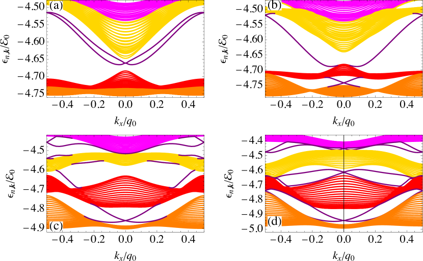
Figure 1: Energies $\epsilon_{n,k_{x}}$ of the energy bands numbered by $n=5$ (orange), $n=6$ (red), $n=7$ (gold), $n=8$ (magenta), for $V_{0}=5\,\mathcal{E}_{0}$, $B_{0}=10\,\mathcal{B}_{0}$, and four values of the external magnetic field $B_{\mathrm{ext}}$: (a) $B_{\mathrm{ext}}=0.05\,\mathcal{B}_{0}$, (b) $B_{\mathrm{ext}}=0.2\,\mathcal{B}_{0}$, (c) $B_{\mathrm{ext}}=0.7\,\mathcal{B}_{0}$, and (d) $B_{\mathrm{ext}}=1.0\,\mathcal{B}_{0}$. Also shown are the edge-state energies (purple) that result when the blue-detuned potential $V_{\mathrm{BD}}(y)(y)=V_{\mathrm{BD},0}\Theta(|y|-L_{y}/2)$ is introduced where $V_{\mathrm{BD},0}$ is taken to be infinite and $L_{y}=25a_{0}$. To experimentally probe high-lying bands and edge states, one would fill the Fermi sea to a desired energy.

The scalar potential $V(\mathbf{r})$ has minima at $\mathbf{r}=\mathbf{a}\equiv n_{1}\mathbf{a}_{1}+n_{2}\mathbf{a}_{2}$ where $n_{1}$ and $n_{2}$ are integers. ${\bf B}_{\mathrm{fic}}({\bf r})$ vanishes at $\mathbf{r}=\mathbf{a}$, and at the edges of the Wigner-Seitz cells, $\mathbf{r}=\mathbf{a}+\tfrac{1}{2}\mathbf{a}_{1}$ and $\mathbf{r}=\mathbf{a}+\tfrac{1}{2}\mathbf{a}_{2}$. Hence the minimum of $V(\mathbf{r})$ at $\mathbf{a}$ [where $V(\mathbf{a})=-2V_{0}$] and the nearest-neighbor minima at $\mathbf{a}+{\bf a}_{j}$ ($j=1,2$) are separated by a barrier of height $V_{0}$. Hence, the bands with $\epsilon_{n,\mathbf{k}}<-V_{0}$ can be well described using a tight-binding model. However, for the bands which are above the barriers, $\epsilon_{n,{\bf k}}>-V_{0}$, tight-binding is a poor approximation. All the bands shown in Fig. 1 are above $-V_{0}$, hence tight-binding cannot be used for them.

Note that nonlinear interactions of ⁶Li, $4\pi\hbar^{2}a_{S}/M$, are weak because the s-wave scattering length $a_{S}=(34\pm 5)a_{0}$ (where $a_{0}$ is the Bohr radius) is small [20]. Hence a single particle picture can be used.

Chern numbers: We determine Chern numbers for the Li atom bands in the SDOLP. Chern numbers are defined on the dispersion bands in wavevector space [1, 4]. For a 2D periodic system, the Chern number $C_{n}$ for the $n$th band is the integration of the Berry curvature, $\mathcal{F}_{xy}(n,{\bf k})=\partial_{k_{x}}A_{y}(n,{\bf k})-\partial_{k_{y}}A_{x}(n,{\bf k})$, over the first BZ,

$$C_{n}=\frac{1}{2\pi}\int_{\rm BZ}d{\bf k}\left(\frac{\partial A_{y}(n,{\bf k})}{\partial k_{x}}-\frac{\partial A_{x}(n,{\bf k})}{\partial k_{y}}\right),$$ (4)

where $A_{\mu}(n,{\bf k})=-i\langle n,{\bf k}|\frac{\partial}{\partial k_{\mu}}|n,{\bf k}\rangle$ is the Berry connection. Expression (4) is formally equivalent to the Berry phase [1, 21, 22] with the difference that the latter can have an integration range which is a subset of the BZ. An efficient method to numerically compute Chern numbers has been proposed in Ref. [23]. One first calculates the link variables $U_{{\bf k}^{\prime},{\bf k}^{\prime\prime}}(n,{\bf k})={\mathrm{Tr}}[\langle n,{\bf k}^{\prime})|n,{\bf k}^{\prime\prime}\rangle]$ for the $n$th Bloch band and normalizes them to unity. Wavevectors ${\bf k}^{\prime}$ and ${\bf k}^{\prime\prime}$ belong to the set $\{{\bf k},{\bf k}+\hat{{\bf k}}_{x},{\bf k}+\hat{{\bf k}}_{y},{\bf k}+\hat{{\bf k}}_{x}+\hat{{\bf k}}_{y}\}$, where $\hat{{\bf k}}_{\mu}$ is a unit vector in direction $\mu$. The curvature $\mathcal{F}_{xy}(n,{\bf k})$ is then given by [23]

$$\mathcal{F}_{xy}(n,{\bf k})=\ln\,\frac{U_{{\bf k},{\bf k}+\hat{{\bf k}}_{x}}(n,{\bf k})\,U_{{\bf k}+\hat{{\bf k}}_{x},{\bf k}+\hat{{\bf k}}_{x}+\hat{{\bf k}}_{y}}(n,{\bf k})}{U_{{\bf k},{\bf k}+\hat{{\bf k}}_{y}}(n,{\bf k})\,U_{{\bf k}+\hat{{\bf k}}_{y},{\bf k}+\hat{{\bf k}}_{x}+\hat{{\bf k}}_{y}}(n,{\bf k})}.$$ (5)

Finally, the Chern numbers are found from the formula $C_{n}=(2\pi\,i)^{-1}\sum_{{\bf k}\in{\rm BZ}}\mathcal{F}_{xy}(n,{\bf k})$, where the sum is evaluated numerically [23].

Increasing the strength of the external magnetic field we find a sequence of topological phase transitions. Phase transitions occur when bandgaps between Bloch bands close and open. The energy gap can vanish at several points in the BZ: the $\Gamma$ point, the vertices of the BZ, and the centers of the edges of the BZ. Some of the gapless spectra have Dirac cones and some have quadratic wavevector dependence. The summary of all topological phase transitions found for external magnetic fields $B_{\mathrm{ext}}<2\,\mathcal{B}_{0}$ is given in the supplementary material (SM) [24]. The lowest critical points at which the topological phase transitions occur are $\{B_{c,1},B_{c,2},B_{c,3},B_{c,4},B_{c,5}\}=\{0.11,0.66,0.89,1.25,1.35\}\mathcal{B}_{0}$. All the Chern numbers vanish below $B_{c,1}$. At the lowest topological phase transition the gap between the $6$th and $7$th bands closes at the center of the BZ and forms a Dirac cone, see Fig. 2. For $B_{c,1}<B_{\mathrm{ext}}<B_{c,2}$, $C_{6}=-1$ and $C_{7}=1$. Indeed, in this case the bulk-boundary correspondence leads to the appearance of two topologically protected chiral edge states in the bandgap, see discussion below. Above $B_{c,2}$ the second topological phase transition appears and the gap between $7$th and $8$th energy bands closes, again at ${\bf k}={\bf 0}$, and $C_{7}$ changes from $+1$ to $-1$, and $C_{8}$ changes from $0$ to $+2$. Note that the sum of all the Chern numbers in the eight lowest energy bands is always equal to zero.

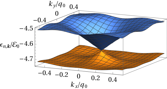
Figure 2: The $6$th and $7$th Bloch bands at the external magnetic field $B_{\mathrm{ext}}=B_{c,1}$. The bands form a Dirac cone at ${\bf k}={\bf 0}$ so the gap between bands is closed at this value of $B_{\mathrm{ext}}$.

Since the Chern numbers $C_{n}$ are non-zero, this system is a topological insulator. For abelian topological insulators, the Chern numbers $C_{n}=-C_{n+1}$, and the number of chiral edge states on each edge between bands $n$ and $n+1$ is $|C_{n}|$ [1, 3]. For non-abelian topological insulators the bulk-edge correspondence is more subtle than the abelian case [25]; multiple tangled bulk bandgaps are present and the system supports non-trivial edge states that manifest the non-Abelian TI features.

Edge states: In order to study edge states for the atoms in the SDOLP we introduce a blue-detuned potential of the form $V_{\mathrm{BD}}(y)=V_{\mathrm{BD},0}\Theta(|y|-L_{y}/2)$ where $\Theta(\bullet)$ is the Heaviside Theta function. This potential mimics the effects of a blue-detuned laser that repels atoms from the region $|y|>L_{y}/2$. For convenience we take $V_{\mathrm{BD},0}$ very large so we can apply Dirichlet boundary conditions at the edge. To compute the edge states we again use the Mathematica command NDEigensystem with Dirichlet boundary conditions at $y=\pm L_{y}/2$ and periodic boundary conditions in $x$. Figure 1 shows the edge states of the finite width strip, $|y|\leq L_{y}/2$, as purple curves that lie in the bandgaps (and within the bands) of the fully periodic system. The edge states in Fig. 1(a) are not TES (all the Chern numbers for the bands are zero for $B_{\mathrm{ext}}<B_{c,1}$). The lower set of edge states in Fig. 1(b) that connect bands 5 and 6 are not TES since there is no gap between the 5th and 6th bands. In contrast, the upper set of edge states in Fig. 1(b) that connect bands 6 and 7 are topological (the Chern number $C_{6}=-1$ and $C_{7}=1$ and the other Chern numbers vanish). In Fig. 1(c) there are edge states between the 5th and 6th bands, 6th and 7th, and 7th and 8th bands. The Chern numbers $C_{6}=C_{7}=-1$ and $C_{8}=2$. Hence, the edge states between the 5th and 6th bands are not topological. There is one pair of TES between the 6th and 7th bands, and two pairs between the 7th and 8th bands. The latter two pairs are located between the 7th and 8th bands near the $k_{x}=0$ point, but are not seen well in Fig. 1(c), but are seen in Fig. 1(d). The former pair connecting the 6th and 7th bands is located in the interval $0.3q_{0}<|k_{x}|<0.4q_{0}$. In Fig. 1(d) there are edge states between all the bands. The Chern numbers are $C_{6}=1$, $C_{7}=-3$ and $C_{8}=2$ which implies that the edge states between the 6th and 7th bands and the 7th and 8th bands are topological. This is surprising because it appears that there is no gap between the 6th and 7th bands (for an infinite SDOLP, our calculations show that there is a gap between the 6th and 7th bands for $B_{c,3}<B_{\mathrm{ext}}<B_{c,4}$, but upon introducing the blue-detuned potential $V_{\mathrm{BD}}(y)$, the gap closes – see SM [24]). One pair of edge states between the 6th and 7th bands cross one another at $k_{x}=0$. Another pair near $k_{x}=\pm 0.4\,q_{0}$ are probably a continuation of the edge states between the 5th and 6th bands. The edge states between the 7th and 8th bands contain two pairs.

In an Abelian TI, the nonvanishing Chern numbers $C_{n}$ and $C_{n+1}$ satisfy the equation $C_{n}+C_{n+1}=0$. In both Fig. 1(c) and (d) $C_{6}$, $C_{7}$ and $C_{8}$ are nonvanishing and $C_{6}+C_{7}$ and $C_{7}+C_{8}$ are nonvanishing, but $C_{6}+C_{7}+C_{8}=0$. Hence, there are two tangled bandgaps; thus the TI is non-Abelian.

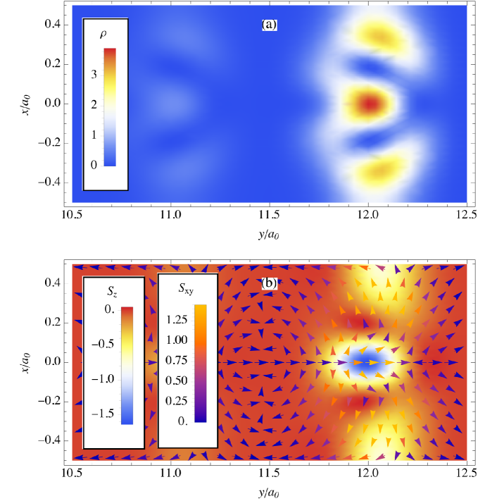
Figure 3: (a) Edge state atom density and (b) spin density for $B_{\mathrm{ext}}=0.2\,\mathcal{E}_{0}/(g_{F}\mu_{B})$ and $k_{x}=-0.2\,q_{0}$ and $L_{y}=25a_{0}$ [see edge state connecting the 6th and 7th bands in Fig. 1(b)]. The colors of the arrows are shown in the $S_{xy}$ legend, and the background color which gives the $S_{z}$ component of the spin density is shown in the left legend.

Not all the edge states shown in purple in Fig. 1 are TES. Only those that connect adjacent bands and lie in the gap between them are TES. The edge states in Fig. 1(a) do not connect different bands and are not topological. Figure 1(b) has edge states that connect the 5th and 6th bands but there is no gap between these bands, hence these edge states are not TES. However, the edge states that connect the 6th and 7th bands have regions in $k_{x}$ that lie in the bandgap; these edge states are TES. The corresponding Chern numbers for the 6th and 7th bands for $B_{c,1}<B_{\mathrm{ext}}<B_{c,2}$ are $C_{6}=-1$ and $C_{7}=1$ respectively. The bulk-boundary correspondence leads to the appearance of one topologically protected chiral edge state in the bandgap on every edge of the topological insulator. Figure 1(c) has edge states that connect the 5th and 6th, 6th and 7th, and 7th and 8th bands. There is no gap between the 5th and 6th bands, hence these edge states are not TES, but there is a pair of TES between the 6th and 7th bands and there are two pairs of TES connecting the 7th and 8th bands. The corresponding Chern numbers for the 6th, 7th and 8th bands for $B_{c,2}<B_{\mathrm{ext}}<B_{c,3}$ are $C_{6}=C_{7}=-1$ and $C_{8}=2$ respectively.

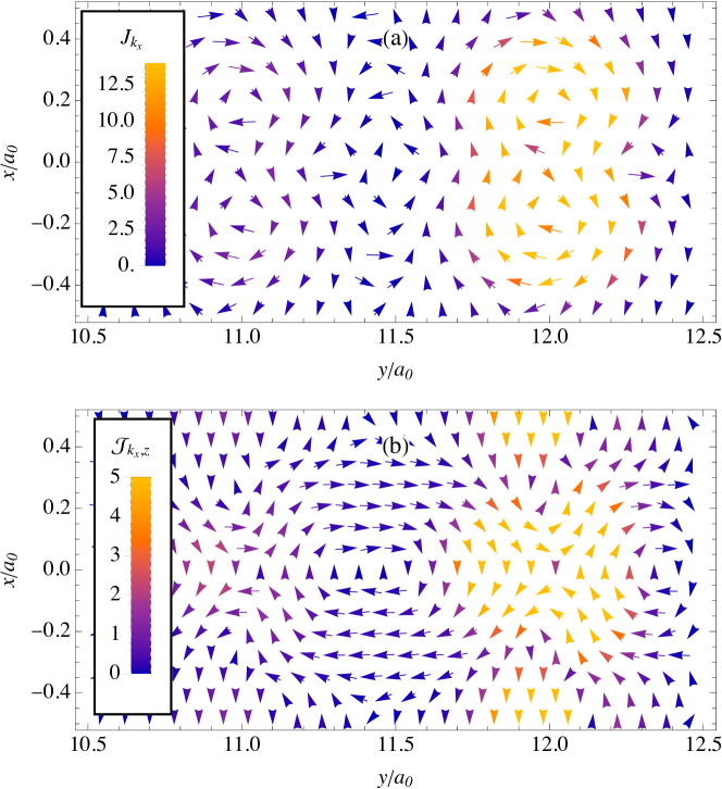
Figure 4: (a) Atom current density $\mathbf{J}_{k_{x}}(\mathbf{r})$ and (b) the spin-current density $\bm{\mathcal{J}}_{k_{x},z}(\mathbf{r})$ for the parameter values used in Fig. 3. Note that the current density flows clockwise, i.e., it has vorticity.

Edge state density, spin density, current density, and spin-current density: The density of a representative edge state with negative $k_{x}$ is shown in Fig. 3(a). The density is restricted to the region near the $y=L_{y}/2$ edge, and the atoms have negative group velocity $v_{g}(k_{x})=\hbar^{-1}d\epsilon/dk_{x}$. The nodes in the edge state density are due to the excited state nature of the edge state. Edge states near $y=-L_{y}/2$ (not shown) have positive $k_{x}$ and positive $v_{g}(k_{x})$. The SM [24] discusses the edge state wave functions.

Figure 3(b) shows the edge state spin density ${\bm{{\mathcal{S}}}}({\bf r})=\psi^{\dagger}_{k_{x}}({\bf r}){\bf F}\psi_{k_{x}}({\bf r})$ (which depends on $k_{x}$), the arrows show the 2-dimensional vector ${\bm{\mathcal{S}}}_{xy}(\mathbf{r})\equiv(\mathcal{S}_{x}(\mathbf{r}),\mathcal{S}_{y}(\mathbf{r}))$, and the color of the arrows show the length $\sqrt{\mathcal{S}_{x}^{2}(\mathbf{r})+\mathcal{S}_{y}^{2}(\mathbf{r})}$. The density plot in Fig. 3(b) shows the $z$-component of the spin density vector, $\mathcal{S}_{z}(\mathbf{r})$ which is negative everywhere except where the wave function has nodes (vortices). The texture of the 2D spin vector ${\bm{\mathcal{S}}}_{xy}(\mathbf{r})$ is due to the $\mathbf{r}$-dependence of $\mathbf{B}_{\mathrm{fic}}(\mathbf{r})$: $\mathcal{S}_{x}({\bf r})$ is an odd function of $x$ since $B_{x,\mathrm{fic}}(\mathbf{r})$ is odd, and $\mathcal{S}_{y}({\bf r})$ is an even function of $x$, since $B_{y,\mathrm{fic}}(\mathbf{r})$ is even. But $\mathcal{S}_{x}({\bf r})$ and $\mathcal{S}_{y}({\bf r})$ have no symmetry with respect to the $y^{\prime}\to-y^{\prime}$ reflection (where $y^{\prime}=12a_{0}-y$) since the edge-state wave function vanishes as a function of $y^{\prime}$ away from the point $\mathbf{r}=(0,12a_{0})$ where the potential has minimum. Additional discussion of edge states and their degeneracy points in $k$-space are presented in the SM [24].

Figure 4(a) shows the atomic current density $\mathbf{J}_{k_{x}}(\mathbf{r})=\tfrac{\hbar}{M}\,\mathrm{Im}\,[\psi_{k_{x}}^{{\dagger}}(\mathbf{r})\,{\bm{\nabla}}\psi_{k_{x}}(\mathbf{r})]$, which can be separated into two parts: $\mathbf{J}_{k_{x}}(\mathbf{r})=J_{k_{x},x}^{\mathrm{av}}(y)\,\hat{\mathbf{x}}+\mathbf{J}_{k_{x}}^{\mathrm{vor}}(\mathbf{r})$. Here $J_{k_{x},x}^{\mathrm{av}}(y)=\tfrac{1}{a_{0}}\int_{-a_{0}/2}^{a_{0}/2}J_{k_{x},x}(\mathbf{r})\,dx$ is an ‘average’ current propagating along the edge of the SDOL, and $\mathbf{J}_{k_{x}}^{\mathrm{vor}}(\mathbf{r})$ which describes a vortex current flow, i.e., a rotational part of the flow. The net atomic current along the edge can be calculated as $J^{\mathrm{tot}}_{k_{x},x}\equiv\int_{-L_{y}/2}^{L_{y}/2}J_{k_{x},x}^{\mathrm{av}}(y)dy$; the total current is negative and depends on $k_{x}$. The total current in the $y$ direction vanishes for all $k_{x}$.

The atomic spin-current density can be denoted by $\mathcal{J}_{k_{x},\alpha,\alpha^{\prime}}(\mathbf{r})=\tfrac{\hbar}{M}\,\mathrm{Im}\,[\psi_{k_{x}}^{{\dagger}}(\mathbf{r})\,F_{\alpha}\partial_{\alpha^{\prime}}\psi_{k_{x}}(\mathbf{r})]$. The subscript $\alpha=x,y,z$, indicates the spin polarization, and the subscript $\alpha^{\prime}=x,y$, specifies the current propagation direction. One can decompose the tensor $\mathcal{J}_{k_{x},\alpha,\alpha^{\prime}}(\mathbf{r})$ into three 2D vectors $\bm{\mathcal{J}}_{k_{x},\alpha}(\mathbf{r})=(\mathcal{J}_{k_{x},\alpha,x}(\mathbf{r}),\mathcal{J}_{k_{x},\alpha,y}(\mathbf{r}))$ which describe spin-polarized currents. Figure 4(b) shows $\bm{\mathcal{J}}_{k_{x},z}(\mathbf{r})$, which has an ‘average’ current along the edge of the SDOL, and vorticity current revealing the rotation of the flow. The non-vanishing total spin-currents are given by $\mathcal{J}^{\mathrm{tot}}_{k_{x},z,x}\equiv\int_{-L_{y}/2}^{L_{y}/2}\mathcal{J}_{k_{x},z,x}^{\mathrm{av}}(y)dy$.

Summary: We studied topological properties of an ensemble of cold fermionic Li atoms in a 2D SDOLP in the presence of an external magnetic field perpendicular to the lattice. Both scalar and vector (fictitious magnetic field) potentials are inherently built into the SDOLP, and both magnetic fields break time-reversal symmetry (see SM [24]). Topological phases, protected by spatial symmetries, appear with increasing external magnetic field. The calculated Chern numbers for the lowest energy bands ($n\leq 8$) are all zero for $B_{\mathrm{ext}}<B_{c,1}$. For $B_{\mathrm{ext}}>B_{c,1}$, the Chern numbers take a series of nonzero values as $B_{\mathrm{ext}}$ increases, revealing both Abelian and non-Abelian topological states and topological phase transitions. For a finite width strip lattice, we observe edge states in energy gaps between successive bands, and some of them are topologically protected. Hence, the atoms in the SDOLP behave as a topological insulator. The topologically protected edge states have interesting properties; both the atom current density and spin-current density have vorticity, and an average flow along the edge.

MB was supported by the NCN Grant No. 2019/32/Z/ST2/00016 through the project MAQS under QuantERA, which has received funding from the European Union’s Horizon 2020 research and innovation program under grant agreement No. 731473.

References

- [1] M. Z. Hasan and C. L. Kane, “Colloquium: Topological insulators”, Rev. Mod. Phys. 82, 3045 (2010).
- [2] X.-L. Qi and S.-C. Zhang, “Topological insulators and superconductors”, Rev. Mod. Phys. 83, 1057 (2011).
- [3] J. K. Asbóth, L. Oroszlány, A. Pályi,A Short Course on Topological Insulators, (Springer International Publishing, 2016).
- [4] N. R. Cooper, J. Dalibard, and I. B. Spielman “Topological bands for ultracold atoms”, Rev. Mod. Phys. 91, 015005 (2019).
- [5] N. Goldman, G. Juzelinas, P. Öhberg and I. B. Spielman, “Light-induced gauge fields for ultracold atoms”, Rep. Prog. Phys. 77 126401 (2014).
- [6] C.-K. Chiu, J. C. Y. Teo, A. P. Schnyder, and S. Ryu, “Classification of topological quantum matter with symmetries”, Rev. Mod. Phys. 88, 035005 (2016).
- [7] B. A. Bernevig, T. L. Hughes, and S.-C. Zhang, “Quantum Spin Hall Effect and Topological Phase Transition in HgTe Quantum Wells”, Science 314, 1757 (2006).
- [8] M. König, S. Wiedmann, C. Brüne, A. Roth, H. Buhmann, L. W. Molenkamp, X.-L. Qi, and S.-C. Zhang, “Quantum spin hall insulator state in HgTe quantum wells”, Science 318, 766 (2007).
- [9] D. Hsieh, D. Qian, L. Wray, Y. Xia, Y. S. Hor, R. J. Cava, and M. Z. Hasan, Nature (London) 452, 970 (2008).
- [10] D. Hsieh, Y. Xia, D. Qian, L. Wray, J. H. Dil, F. Meier, J. Osterwalder, L. Patthey, J. G. Checkelsky, N. P. Ong, A. V. Fedorov, H. Lin, A. Bansil, D. Grauer, Y. S. Hor, R. J. Cava, and M. Z. Hasan, Nature (London) 460, 1101 (2009).
- [11] Y. Xia, D. Qian, D. Hsieh, L. Wray, A. Pal, H. Lin, A. Bansil, D. Grauer, Y. S. Hor, R. J. Cava, and M. Z. Hasan, Nat. Phys. 5, 398 (2009).
- [12] H. Zhai, Rep. Prog. Phys. 78, 026001 (2015).
- [13] J. Dalibard, Quantum Matter at Ultralow Temperatures edited by M. Inguscio, W. Ketterle, and S. Stringari (IOS Press, Amsterdam, 2016).
- [14] M. Aidelsburger, S. Nascimbene, and N. Goldman, C. R. Physique 19, 394 (2018).
- [15] I. Kuzmenko, T. Kuzmenko, Y. Avishai, and Y. B. Band, “Atoms trapped by a spin-dependent optical lattice potential: Realization of a ground-state quantum rotor”, Phys. Rev. A 100, 033415 (2019).
- [16] P. Szulim, M. Trippenbach, Y. B. Band, M. Gajda, and M. Brewczyk, “Atoms in a spin dependent optical potential: ground state topology and magnetization”, New J. Phys. 24, 033041 (2022).
- [17] F. Le Kien, P. Schneeweiss, and A. Rauschenbeutel, “Dynamical polarizability of atoms in arbitrary light fields: general theory and application to cesium”, Eur. Phys. J. D 67, 92 (2013).
- [18] C. Cohen-Tannoudji and J. Dupont-Roc, “Experimental Study of Zeeman Light Shifts in Weak Magnetic Fields”, Phys. Rev. A 5, 968 (1972).
- [19] A. M. Dudarev, R. B. Diener, I. Carusotto, and Q. Niu, “Spin-Orbit Coupling and Berry Phase with Ultracold Atoms in 2D Optical Lattices”, Phys. Rev. Lett. 92, 153005 (2004).
- [20] E. R. I. Abraham, W. I. McAlexander, J. M. Gerton, R. G. Hulet, R. Côtè, and A. Dalgarno “Singlet s-wave scattering lengths of 6Li and 7Li” Phys. Rev. A53, R3713 (1996).
- [21] M. V. Berry, “Quantal Phase Factors Accompanying Adiabatic Changes”, Proc. R. Soc. Lond. 392, 45 (1984).
- [22] S. Rachel, “Interacting topological insulators: a review”, Rep. Prog. Phys. 81, 116501 (2018).
- [23] T. Fukui, Y. Hatsugai, and H. Suzuki, “Chern Numbers in Discretized Brillouin Zone: Efficient Method of Computing (Spin) Hall Conductances”, J. Phys. Soc. Jpn. 74, 1674 (2005).
-
[24]
I. Kuzmenko, M. Brewczyk, G. Łach, Y. B. Band, and M. Trippenbach,
“Supplementary materials: Atoms in a spin-dependent optical lattice potential as a topological insulator with broken time-reversal symmetry”, https
Supplementarymaterials. - [25] T. Jiang , R.-Y. Zhang, Q. Guo, B. Yang, and C. T. Chan, “Two-dimensional non-Abelian topological insulators and the corresponding edge/corner states from an eigenvector frame rotation perspective”, Phys. Rev. B 106, 235428 (2022).