Reconstructing cryptocurrency processes via Markov chains

Abstract

The growing attention on cryptocurrencies has led to increasing research on digital stock markets. Approaches and tools usually applied to characterize standard stocks have been applied to the digital ones. Among these tools is the identification of processes of market fluctuations. Being interesting stochastic processes, the usual statistical methods are appropriate tools for their reconstruction. There, besides chance, the description of a behavioural component shall be present whenever a deterministic pattern is ever found. Markov approaches are at the leading edge of this endeavour. In this paper, Markov chains of orders one to eight are considered as a way to forecast the dynamics of three major cryptocurrencies. It is accomplished using an empirical basis of intra-day returns. Besides forecasting, we investigate the existence of eventual long-memory components in each of those stochastic processes. Results show that predictions obtained from using the empirical probabilities are better than random choices.

Keywords: Markov chains, Cryptocurrency, Forecasting, Market Processes

JEL Classification D8, H51

1 Introduction

Since the introduction of Bitcoin by Nakamoto (2008), cryptocurrencies have received considerable attention from monetary authorities, firms and investors. The reasons for all this attention are the possibility of reducing risk management, improving portfolios and analyzing consumer sentiment (Dyhrberg, 2016). Indeed, few financial innovations have drawn similar attention from regulators, investors and stakeholders.

Attention naturally led to characterizing some stylized facts of the digital market. References Urquhart (2017) and Cunha, C.R. & Silva, R. (2020) show that stylized facts of Bitcoin (BTC) data are similar to those of traditional financial assets. Namely, distributions of BTC one-day returns display fat tails, exhibit volatility clustering and the correlation between its volume and volatility is always positive. Reference Cheah et al.(2018) uses daily data to model the volatility in the cryptocurrency market. Their findings indicate that the cryptocurrencies studied (Bitcoin, Ethereum and Ripple) have long memory. Likewise, Kaya et al. (2020) show that those cryptocurrencies have fat-tail distributions suggesting that their returns approach three standard deviations.

Simultaneously, Bariviera (2017) focus on studying BTC long-range memory of daily and intra-day prices. The authors show that BTC data display high volatility, long-range memory unrelated to market liquidity, and intra-day prices similar across different time scales (5 to 12 hours). Moreover, the persistent behavior of daily prices from 2011 to 2014 was captured by the calculation of the Hurst exponent, showing that, after 2014, it decreased to nearly $0.5$, behaving like a random process. Malladi, R.K. & Prakash L.D. (2021), analyze the returns and volatility of BTC and Ripple (XRP). They found that returns of global stock markets and gold do not have a causal effect on BTC returns. However, the returns of cryptocurrencies with less market capitalization, like XRP, are more affected by gold prices and stock market volatility. Since the prices of XRP are more volatile and more affected by market news, the authors use its prices as a proxy for investor fear and show that its volatility can also drive BTC prices.

Likewise, references Dyhrberg (2016) and Baur (2010) show that BTC has similar hedging capabilities to gold against the US dollar and the Stock Exchange Index. Their arguments rely on hedging capabilities, concluding that investors can use this virtual currency alongside gold to eliminate or minimize specific market risks. In addition, as BTC can be traded continuously, 24 hours per day and seven days per week, Dyhrberg (2016) argues that this virtual currency has specific speed advantages and can be added to the list of hedging tools. Similarly, Deniz, A. & Teker, D. (2020), show that BTC and Gold price series are cointegrated, implying that both series follow similar paths in the long term. They also show, through the Granger test, that gold prices affect BTC prices in a short time. However, these results are different for Ethereum (ETH) and XRP prices, where there is no direct long or/and short-term relation between these price series and gold.

Cheah et al.(2018) show that BTC prices behave like a traditional asset, being prices dominated by highly speculative periods. Therefore, they conclude that the cryptocurrency market shows substantial similarity in stylized empirical facts when compared to traditional markets and, more precisely, in what concerns vulnerability to speculative bubbles. In the same way, Cobert et al. (2018) also study the stochastic properties of the leading cryptocurrencies and their linkages to standard stock market indices. The main findings show that the behavior of cryptocurrency markets is highly connected to each other but decoupled from the primary traditional stock indexes. Therefore, digital stocks are seen as an essential contribution since they offer diversification benefits to investors.

In the present paper, in order to estimate the behavior of some major cryptocurrencies, the processes of one-hour returns of BTC, ETH and XRP are reconstructed. It is done by using Markov chains of orders one to eight. The reconstruction of those cryptocurrencies processes starts with the identification of: (i) the allowed (markovian) transitions in the state space that corresponds to current orbits of the system, and (ii) the occurrence frequency of each orbit in typical samples. It is accomplished by taking the first half ( the past) of each sample to the computation of the conditional probabilities of the allowed transitions. From this empirical base, each second half (the future) is estimated and compared with a random choice. Results show that the predictions obtained from the empirical transitions probabilities outperform random forecasts.

A short overview of the subsequent sections of this paper consists in the following: the next section describes the data used in our empirical approach. Such a description is followed by the presentation of the methodology: a Markov chain model that underlies the reconstruction of three cryptocurrency processes. Section 3 presents and discuss the results obtained from such a reconstruction and compare them with random forecasts. The last section presents and concluding remarks and outlines future work.

2 Data and Methods

The data used in the present study is sourced from coinmarket.com, where historical information about over one thousand cryptocurrencies is available. Three major cryptocurrencies according to their market capitalization: BTC, ETH and XRP were considered. Fig. 1 shows the behavior of hourly-price data for those three digital stocks.

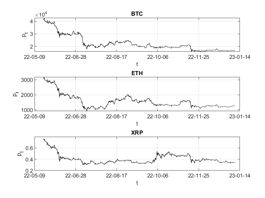
Figure 1: Hourly-prices $p_{t}$ of the three cryptocurrencies, from May-20-2022 to Jan-08-2023.

The three plots in Fig.1 present the series of hourly-prices of BTC, ETH and XRP, from May-20-2022 to Jan-08-2023, comprising each of them 6306 observations.

From the plots in Fig.1, it is quite apparent that the data are very far from stationary, but a different situation comes out when, instead of prices, we considered the series of one-hour returns.

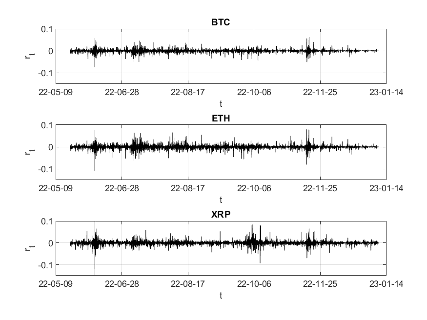
Figure 2: Hourly-returns of the cryptocurrencies, from 2022-05-20 to 2023-01-08

$$r_{t}=log(p_{t})-log(p_{t-1}).$$ (1)

The three plots in Fig.2, show the series the one-hour returns, while the plots in Fig.3 illustrate their dynamics, i.e., the phase spaces of those dynamical systems, as Eq.2 formally states.

$$r\left(t,1\right)\rightarrow r\left(t+1,1\right)$$ (2)

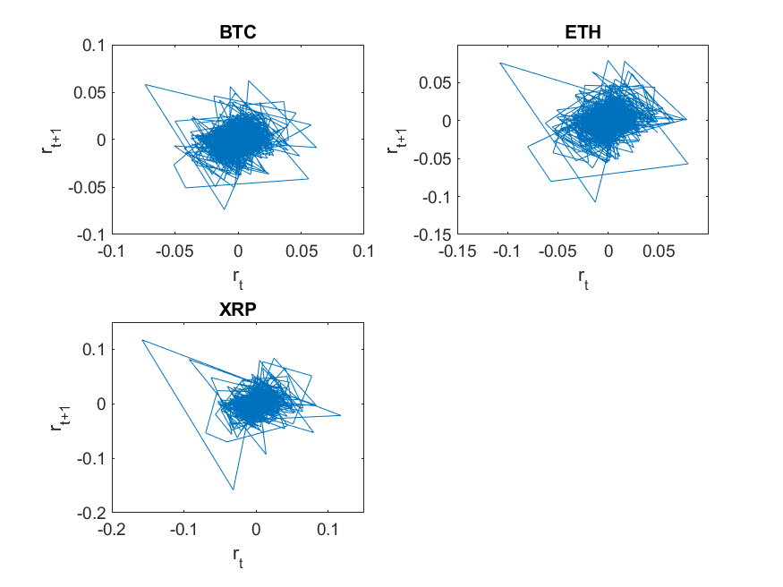
Figure 3: The dynamics of hourly-returns of the three cryptocurrencies, i.e., the phase spaces of those dynamical systems, as Eq.2 formally states.

These last three plots (Fig.3) show that, in the three cases, the bulk of the data consists of a central core of small fluctuations with a few large flights away from the core. This structure of the data will have influence on the results obtained in the next section.

2.1 Markov Chains

There is a huge literature applying Markov Chains to model the behaviour of financial time series. This approach is a fundamental tool in the study of stochastic processes. It has been used widely in many different disciplines, like weather, epidemic, land use, consumer behavior and even for the identification of writers (Khmelev, D.V., & Tweedie, F. J. (2001)).

A sequence of random variables $Z_{1},Z_{2},\ldots,Z_{t},\ldots$ with Markov characteristics is known as a process with first order dependence (as described in Equation 3, this process has no memory). The Markov characteristics means that the distribution of the future realization of $Z_{n+1}$ depends on its immediately previous state ($Z_{n}$) and not on further previous states ($Z_{n-1},Z_{n-2},\ldots$). Formally,

$$Pr(Z_{n+1}=z_{n+1}\mid Z_{1}=z_{1},\ldots,Z_{n}=z_{n})\\ =Pr(Z_{n+1}=z_{n+1}\mid Z_{n}=z_{n})$$ (3)

In a dynamical system, shifting from state $i$ to state $j$ has transition probability $p_{ij}$

$$p_{ij}=Pr(Z_{1}=s_{j}\mid Z_{0}=s_{i})$$ (4)

Fortunately, Markov chains can be approached from a higher order perspective, being Markov chains of higher orders the processes in which the next state depends on two or more preceding ones. Here, Markov chains of orders one to eight are considered as a way to predict cryptocurrency hourly-returns and to investigate the existence of eventual long-memory components in that stochastic process.

2.2 Coding

We consider the dynamical system being coded by a finite alphabet $\Sigma$. Then, $\Omega$, the space of orbits of the system are comprised of infinite sequences $\omega=i_{1}i_{2}\cdots i_{k}\cdots$, $i_{k}\in\Sigma$, with the dynamical law being a shift $\sigma$ on these symbol sequences.

$$\sigma\omega=i_{2}\cdots i_{k}\cdots$$ (5)

Depending on the dynamical law of the coded system, not all sequences will be allowed. The set of allowed sequences in $\Omega$ defines the grammar of the shift. The set of all sequences which coincide on the first $n$ symbols is called a $n-$block and is denoted $[i_{1}i_{2}\cdots i_{n}]$. The probability measures over the $n-$blocks constitute part of information that may be inferred from the data, being the main tool used to characterize the dynamical properties of the dynamical system.

To calculate the probability measures over the $n-$blocks the following computation is performed: for each series of one-hour returns ($r_{t}$) with mean $\hat{r}$ and standard deviation $s$, a five-symbols code $\Sigma$ is defined.

$$\Sigma=\left\{-2,-1,0,1,2\right\}$$ (6)

Then,

$$\begin{array}[]{clc}\left(r\left(t\right)-\overline{r\left(t\right)}\right)>s&\Longleftrightarrow&2\\ s\geq\left(r\left(t\right)-\overline{r\left(t\right)}\right)>\frac{s}{3}&\Longleftrightarrow&1\\ \frac{s}{3}\geq\left(r\left(t\right)-\overline{r\left(t\right)}\right)>-\frac{s}{3}&\Longleftrightarrow&0\\ -\frac{s}{3}\geq\sigma\left(r\left(t\right)-\overline{r\left(t\right)}\right)>-s&\Longleftrightarrow&-1\\ -s\geq\left(r\left(t\right)-\overline{r\left(t\right)}\right)&\Longleftrightarrow&-2\end{array}$$ (7)

This coding is used and the empirical frequencies $\widetilde{\mu}\left([i_{1}\cdots i_{k}]\right)$ for blocks of successively larger order $k$ are found. Naturally, $k$ cannot be arbitrarily large because of statistics. The reliability of results is threatened whenever $5^{k}$ is larger than the size $N$ of the data sample. Therefore, statistical reliability may be directly tested by comparing the number of different occurring blocks and $5^{k}$.

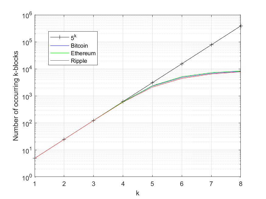
Figure 4: Comparing the number of different occurring blocks of size $k$ and $5^{k}$

Fig.4 shows the evolution of the number of occurring $k-$blocks and $5^{k}$, where the number $p\left(k\right)$ of occurring blocks of size $k$ in each data sample is compared with the maximum possible number, $5^{k}$. In all cases, after $k=4$ the comparison shows the lack of statistics apparent in the comparison of $p\left(k\right)$ with $5^{k}$. These results seem to suggest that the data are described by a short range memory.

2.3 Predicting

Prediction starts by taking the time series of each cryptocurrency and spliting the series into two halves, the first half is then used to predict the other half. The coding procedure presented in the last section is used and after the first half of each sample is coded into $\Sigma=\left\{-2,-1,0,1,2\right\}$, we perform the computation of the conditional probabilities of the allowed transitions on these symbol sequences. The conditional probabilities are computed for blocks of successively larger order ($k$).

As an example, the conditional probabilities computed for blocks of size two are defined in the following Markov transition matrix.

$$P=\left[{\begin{array}[]{ccccc}p_{11}&p_{12}&p_{13}&p_{14}&p_{15}\\ p_{21}&p_{22}&p_{23}&p_{24}&p_{25}\\ p_{31}&p_{32}&p_{33}&p_{34}&p_{35}\\ p_{41}&p_{42}&p_{43}&p_{44}&p_{45}\\ p_{51}&p_{52}&p_{53}&p_{54}&p_{55}\\ \end{array}}\right]$$

where each $p_{ij}$ indicates the probability of shifting from state $i$ to state $j$, as in Equation 3.

The transition matrices for blocks of orders up to eight are computed. From this empirical base, each second half is estimated and compared with a random number chosen at random.

However, when the conditional probabilities are inferred from limited experimental data an extended Markov approximation is more convenient, we used the Less-than-$k$-Markov approach as defined by Vilela-Mendes et al. (2002).

2.3.1 The Less-than-$k$-Markov approach

In each simulation, with an approximation of order $k$, we look at the current block $\left(a_{1}\cdots a_{k}\right)$ of order $k$ and use the $k-$empirical probability to infer the next state $a_{0}$. If that block is not present in the data that were used to construct the empirical probabilities, then we look at the $k-1$ sized block $a_{1}\cdots a_{k-1}$ and use the $k-1$ order empirical probabilities. If required, the process is repeated until an available empirical probability given by a $(k-i)-$order block with $2<i<8$ is found.

Such an extended Markov approach is applied to each $k-$order block in order to estimate the successor $a_{0}$ of each block $\left(a_{1}\cdots a_{k}\right)$. In so doing, the successor $a_{0}$ is compared with a prediction $\widetilde{a}_{0}$ obtained by throwing a random number with the empirical probabilities $\widetilde{P}\left(a_{0}\mid a_{1}\cdots a_{k}\right)$.

The Past predicting the future

Once the empirical probabilities are computed from the first half of each series ($t=1,2,...n$) the second half is visited ($t=n+1,n+2,...2n$) in order to quantify the magnitude of the error found when using each $k-$sized block, the quantity $e_{k}(t)$ is computed for each sample: BTC, ETH and XRP.

$$e_{k}(t)=[\widetilde{a}_{0}-a_{0}(t)]$$ (8)

As half of each series comprises $n$ observations, the averaged error for each $k-block$ is calculated

$$e_{k}=\frac{1}{n}\sum_{t=n+1}^{2n}[\widetilde{a}_{0}-a_{0}(t)]$$ (9)

The average error of the forecast of the second half of each sample is therefore computed as the distance between the observed $a_{0}$ and the corresponding estimated state $\widetilde{a}_{0}$.

The same procedure is performed with the successor $a_{0}$ of each $k-$order block being estimated at random ($\widetilde{r_{0}}$). There, the error is given by the distance

$$eRand_{k}=\frac{1}{n}\sum_{t=n+1}^{2n}[\widetilde{r_{0}}-a_{0}(t)]$$ (10)

In the end, the errors $e_{k}$ and $eRand_{k}$ are averaged over 50 different runs.

2.4 Method outline

In the following, a brief and summarized description of the algorithm used in the simulations is presented. The final results contain average values over 50 runs for each cryptocurrency.

Outline of the algorithm

Take each cryptocurrency series of hourly-prices: BTC, ETH or XRP

1. Compute hourly-returns: $r_{t}=log(p_{t})-log(p_{t-1})$ from the series of prices $p_{t}$ (Eq.1)

2. Split the series of returns into two halves of the same size $n$: $H_{1}$ and $H_{2}$

3. Code the two halves $H1$ and $H2$ into $\Sigma=\left\{-2,-1,0,1,2\right\}$ (Eq.7)

4. Perform the steps (4.1 to 4.5) along $j=1,2,...,50$ simulations:

   1. For each $k-block$ successively larger $k=2,...,8$

      1. 4.1 Build the conditional probabilities $\widetilde{P}[(a_{0}[a_{1}\cdots a_{k}])$

      2. 4.2 Look at the $k$ sized block $a_{1}\cdots a_{k}$ and use the $k$ order empirical probabilities to infer each next state $a_{0}$ with

      3. $\Diamond$ If the block $a_{1}\cdots a_{k}$ is not found, repeat using blocks of size $(k-\i)$ with $2<i<k$ until the available empirical probability is found

      4. 4.3 Visit each ${a}_{0}(t)\in H2$, $t=n+1,n+2,...2n$

      5. 4.4 Measure the error $e_{k}(j)=\frac{1}{n}$$(\sum_{t=n+1}^{2n}[a_{0}(t)-\widetilde{a}_{0}]$) (Eq.8)

      6. 4.5 Compute $eRand_{k}(j)=\frac{1}{n}(\sum_{t=n+1}^{2n}[a_{0}(t)-r_{0}]$ ) being $r_{0}$ chosen at random (Eq.9)

5. Compute the average errors $e_{k}$ and $eRand_{k}$ over $j=1,2,...,50$ simulations (Eq.10)

   1. $\bullet$ $e_{k}=\frac{1}{50}\sum_{j=1}^{50}e_{k}(j)$

   2. $\bullet$ $eRand_{k}=\frac{1}{50}(\sum_{j=1}^{50}eRand_{k}(j)$)

3 Results and Discussion

The first three plots in Fig. 5, show the average error obtained with a 5-symbols alphabet for the three cryptocurrencies. The last plot shows the error obtained for each cryptocurrency and computed when the prediction is performed at random, i.e., from a surrogate matrix of probabilities.

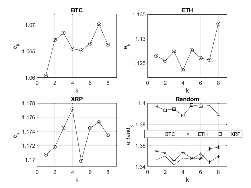
Figure 5: The first half of each sample (the past) predicting the second half (the future), using a 5-symbols alphabet.

These results are similar to those obtained by Vilela-Mendes et al. (2002) where daily returns of three standard stocks and the NYSE index were analysed. Not surprisingly, in all cases, the average prediction obtained from using the empirical probabilities is better than a random choice. However, here, ETH and XRP data show even higher improvements coming from the four and five-symbol blocks, respectively.

The stocks BTC and ETH seem to share closer similarities than any of them with XRP. However, the one-symbol probabilities are similar in the three digital stocks. This suggests that the statistical short-memory component of the market process might be similar for many different stocks, whether for the long-memory component such a similarity might be lost.

As already mentioned in the previous section, statistical limitations underlie the improvements obtained by using higher order blocks, showing much larger fluctuations.

Results previously obtained (Vilela-Mendes et al., 2002) and the need to further characterize the presence of small and large fluctuations, led to the application of the same method, with same data samples being coded by a 3-symbol alphabet. As before, $s$ is the standard deviation of the hourly-returns samples.

$$\Sigma=\left\{-1,0,1\right\}$$ (11)

Then,

$$\begin{array}[]{clc}\left(r\left(t\right)-\overline{r\left(t\right)}\right)>s&\Longleftrightarrow&1\\ s\geq\left(r\left(t\right)-\overline{r\left(t\right)}\right)>s&\Longleftrightarrow&0\\ -s\geq\left(r\left(t\right)-\overline{r\left(t\right)}\right)&\Longleftrightarrow&-1\end{array}$$ (12)

When this shorter code is adopted, the number of large events is the same as before being the statistics of small fluctuations improved. The method is the same with the single replacement of the 5-symbol alphabet by the new one $\Sigma=\{-1,0,1\}$ with just three symbols.

The first three plots in Fig.6 show the average error obtained with a 3-symbols alphabet for the three cryptocurrencies. The last plot shows the error obtained for each cryptocurrency and computed when the prediction is performed at random, i.e., from a surrogate matrix of probabilities.

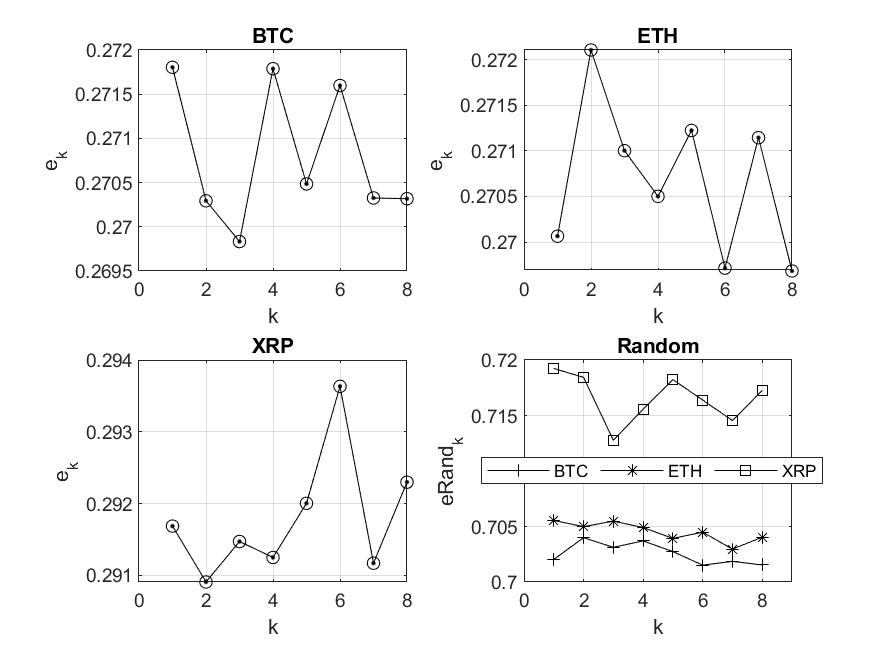
Figure 6: The first half of each sample (the past) predicting the second half (the future), using a 3-symbols alphabet.

Results show a prediction improvement extending to block sizes larger than before (with the 5-symbol alphabet). Because small fluctuation errors are decreased by better statistics, the persistence of the improvement for larger blocks seems to highlight the presence of a long-memory component. Again, the stocks BTC and ETH seem to share closer similarities than any of them with XRP.

The first two plots Fig.6 show that $e_{k}$ computed for BTC and ETH is equally ranged in the y-axis. On the contrary, $e_{k}$ computed for XRP displays quite different limits. A closer correlation between the first two stocks is also present in the values of $eRand_{k}$ as the last plots in Fig.5 and Fig.6 show.

These difference displayed by XRP fluctuations is certainly related to the much larger flights observed in the dynamics of XRP hourly returns presented in Fig.3. The improvement in the predictions obtained for small-order blocks is similar to those presented in reference Vilela-Mendes et al. (2002), where the dynamics of standard stocks was analyzed. A similar approach has also analyzed the dependence of memory on the dynamics of processes of cryptocurrency daily-returns. There, reference (Nascimento, 2022) - also looking at Bitcoin, Ethereum and Ripple - found the occurrence of long-range memory up to 7-order Markov chains.

4 Conclusions

In this paper, a Markov approach is used to model the fluctuations of processes of hourly-returns of three cryptocurrencies: Bitcoin, Ethereum and Ripple. Markov chains of orders one to eight were considered as a way to predict cryptocurrency returns and to investigate the occurrence of eventual long-memory components in those stochastic processes.

Since conditional probabilities are inferred from limited experimental data, an extended Markov approximation seems to be advantageous. Here, we used the Less-than-$k$-Markov approximation as presented in reference Vilela-Mendes et al. (2002).

The most important result is that the average predictions obtained from using the empirical probabilities outperform a random choice.

The main contributions rely on a predictive approach not yet used for series of cryptocurrencies. Moreover, using hourly data we benefit from better statistics when compared with daily ones but avoiding the inconvenient of high-frequency data (i.e. minute observations) since it involves the interplay of many more reaction time scales and market compositions in the trading process. Therefore, the choice of series of hourly observations seems to be an appropriate way to understand the stochastic process that underlies the market mechanism.

Notice, however, that the trade-off between higher order approximations and the lack of statistics is the main limitation of our approach. Future work is planned to apply the same approach to explore the use of the empirical probabilities of one cryptocurrency to predict the behavior of the others. In so doing, we would be able to understand the strength of connectivity between digital stocks in the behaviour of the cryptocurrency market.

Acknowledgments

This article is part of the Strategic Project UIDB050692020. The authors acknowledge financial Support from FCT – Fundação para a Ciência e Tecnologia (Portugal).

References

• Bariviera, A.F., Basgall, M.J., Hasperue, W. & Naiouf, M. (2017). Some Stylized Facts of the Bitcoin Market. Physica A: Statistical Mechanics and Its Applications 484: 82–90.
  https://doi.org/10.1016/j.econlet.2015.02.029.

• Baur, D. & Lucey, B.M. (2010). Is Gold a Hedge or a Safe Haven? An Analysis of Stocks, Bonds and Gold. Financial Review 45 (2): 217–29.
  https://doi.org/10.1111/j.1540-6288.2010.00244.x.

• Cheah, E.T., Mishra, T., Parhi, M. & Zhang, Z. (2018), Long memory interdependency and inefficiency in bitcoin markets, Economics Letters, 167, 18–25.

• Corbet, S., Meegan, A., Larkin, C., Lucey, B. & Yarovaya, L. (2018), Exploring the dynamic relationships between cryptocurrencies and other financial assets, Economics Letters, 165, 28–34.
  https://doi.org/10.1016/j.econlet.2018.01.00

• Cunha, C.R. & Silva, R. (2020). Relevant Stylized Facts about Bitcoin: Fluctuations, First Return Probability, and Natural Phenomena. Physica A: Statistical Mechanics and Its Applications, 550: 124–55. https://doi.org/10.1016/j.physa.2020.124155.

• Dyhrberg, A.H. (2016). Hedging Capabilities of Bitcoin. Is It the Virtual Gold? Finance Research Letters 16: 139–44.
  https://doi.org/10.1016/j.frl.2015.10.025.

• Kaya, P., Okur, M., Ozgur C., & Altintig, Z. A. (2020), 2020. Long Memory in the Volatility of Selected Cryptocurrencies: Bitcoin, Ethereum and Ripple. Journal of Risk and Financial Management 13 (6): 107.

• Khmelev, D.V. & Tweedie, F. J. (2001). Using Markov Chains for Identification of Writer. Literary and Linguistic Computing 16 (3): 299–307.
  https://doi.org/10.1093/llc/16.3.299.

• Malladi, R.K. & Prakash L.D. (2021). Time Series Analysis of Cryptocurrency Returns and Volatilities. Journal of Economics and Finance 45 (1): 75–94.

• Nakamoto, S. (2008). Bitcoin: A Peer-to-Peer Electronic Cash System. Decentralized Business Review, 212–60.
  https://papers.ssrn.com/sol3/papers.cfm

• Nascimento, F., Santos, S., Silva J., Alves, X. & Ferreira, T. (2022). Extracting Rules via Markov Chains for Cryptocurrencies Returns Forecasting. Computational Economics, 1–20.
  https://doi.org/10.1007/s10614-022-10237-7.

• Urquhart, A. (2017), Price clustering in bitcoin, Economics letters, 159, 145–148.
  https://doi.org/10.1016/j.econlet.2017.07.035.

• Vilela-Mendes, R., Lima, R. & Araujo, T. (2002). A Process-Reconstruction Analysis of Market Fluctuations. International journal of Theoretical Applied Finance 5 (08): 797–821.
  http://doi.org/10.1142/S0219024902001730.

Declarations

• Funding
  This article is part of the Strategic Project UIDB/05069/2020. The authors acknowledge financial Support from FCT – Fundação para a Ciência e Tecnologia (Portugal).

• Conflict of interest/Competing interests The authors have no conflicts of interest to declare that are relevant to the content of this article.

• Ethics approval: Not applicable

• Consent to participate: Not applicable

• Consent for publication: Not applicable

• Availability of data and materials Data are available at coinmarket.com

• Code availability Code will be available at a GitHub public repository.

• Authors’ contributions

  T. Araújo : Methodology, Software, Supervision, Writing-Reviewing and Editing.
  P. Barbosa: Data mining, Software, Writing - Original draft preparation.