On the lower bound of the Heisenberg uncertainty product in the Boltzmann states

Abstract

The uncertainty principle lies at the heart of quantum mechanics, as it describes the fundamental trade-off between the precision of position and momentum measurements. In this work, we study the quantum particle in the Boltzmann states and derive a refined lower bound on the product of $\Delta x$ and $\Delta p$. Our new bound is expressed in terms of the ratio between $\Delta x$ and the thermal de Broglie wavelength, and provides a valuable tool for characterizing thermodynamic precision. We apply our results to the Brownian oscillator system, where we compare our new bound with the well-known Heisenberg uncertainty principle. Our analysis shows that our new bound offers a more precise measure of the thermodynamic limits of precision.

Introduction.

The uncertainty principle is a cornerstone of quantum mechanics, expressing the fundamental limitation on our ability to simultaneously measure certain pairs of physical observables Hei49 . The most well–known version of the uncertainty principle is the Heisenberg uncertainty relation, which places a lower bound on the product of the standard deviations of position and momentum for a quantum particle Hei27172 . It reads

$$\Delta x\Delta p\geq\frac{\hbar}{2},$$ (1)

where $\Delta x\equiv\sqrt{\langle\delta\hat{x}\delta\hat{x}\rangle}$, $\Delta p\equiv\sqrt{\langle\delta\hat{p}\delta\hat{p}\rangle}$ and $\hbar$ is the reduced Planck constant. Equation (1) holds for any quantum pure or mixed state, giving a universal lower bound of the Heisenberg uncertainty product $\Delta x\Delta p$. It is also usually interpreted as some upper limit to the precision of our measurements in microscopic world and inspires a lot of studies and discussions on this thread; see e.g. Ref  Bus07155 ; Rud1238003 ; Roz12100404 ; Bao205658 ; Has232828 .

In recent years, there has been growing interest in understanding the precision of observables in quantum thermodynamic regimes Lee18032119 ; Bra18090601 ; Has19110602 ; Tim19090604 ; Sei19176 ; Has19062126 ; Gua19033021 ; Hor2015 ; Van22140602 ; Fu22024128 ; Kam23L052101 . Especially, when in the equilibrium Boltzmann state, the system density operator is then proportional to $\exp(-\beta\hat{H})$ with $\beta\equiv 1/(k_{B}T)$ being the inverse temperature and $\hat{H}$ the Hamiltonian. One natural question arises: Can the lower bound of the Heisenberg uncertainty product $\Delta x\Delta p$ be refined when the system is constrained in the Boltzmann equilibrium state?

On the other hand, when the thermodynamic effects are involved at finite temperatures, the thermal de Broglie wavelength,

$$\lambda_{\rm th}\equiv\sqrt{\frac{2\pi\hbar^{2}}{mk_{B}T}},$$ (2)

can be roughly viewed the average de Broglie wavelength of particles, where $m$ is the mass of the particle Hua87 ; Cha87 . It describes the wave–like nature of particles at certain temperatures. At higher temperatures, particles have greater kinetic energy, which leads to shorter thermal de Broglie wavelengths. Therefore, the thermal de Broglie wavelength is crucial for predicting and analyzing the behavior of particles under different temperatures. For example, when $\lambda_{\rm th}\sim n^{-1/3}$ with $n$ the particle number density, the quantum effect is anticipated to be prominent Hua87 ; Cha87 . So, another question comes: How shall we connect $\lambda_{\rm th}$ to the thermodynamic uncertainty of precision?

In this work, we report on the discovery of a refined lower bound, named as the Boltzmann lower bound, of the Heisenberg uncertainty product in the Boltzmann states. The uncertainty relation is then expressed as

$$\Delta x\Delta p\geq\frac{\hbar}{2}\times\Gamma\Big{(}\frac{1}{4\pi r^{2}}\Big{)}\ \ \text{with}\ \ r\equiv\Delta x/\lambda_{\rm th}.$$ (3)

Here, $\Gamma(x)>1$ is a constructed function reading

$$\Gamma(x)=\frac{g^{-1}(x)}{x},$$ (4)

where $g^{-1}$ is the inverse function of $g(x)=x\tanh(x/2)$. In Eq. (3), $r$ is defined as the ratio of $\Delta x$ to the thermal de Broglie wavelength. Generally, Eq. (3) supplies us with a lower bound that is encoded with both the quantum ($\hbar$) and thermodynamic ($\lambda_{\rm th}$) features; see Fig. 1.

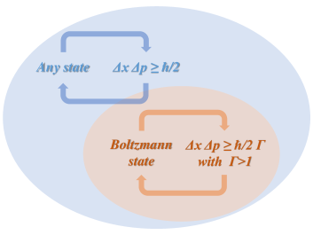
Figure 1: An illustrative figure of Heisenberg lower bound (in light blue) [cf. Eq. (1)] versus Boltzmann lower bound (in orange) [cf. Eq. (3)].

The remainder of this paper is organized as follows. Next, we present the step–by–step derivation of the Boltzmann lower bound in Eq. (3). The demonstration and discussion are then carried out on the Brownian oscillator system, including the comparison with the celebrated lower bound of Heisenberg. Finally, we summarize the paper.

Boltzmann lower bound.

In this section, we will present the step–by–step derivation of Eq. (3). The methodology here is closely related to that exploited in deriving thermodynamic uncertainty relations Str22 .

Step 0: Notations and preliminary knowledge. For later use, we denote

$$c(t)\equiv\langle\delta\hat{x}(t)\delta\hat{x}(0)\rangle,$$ (5)

where the average $\langle(\,\cdot\,)\rangle$ runs over the Boltzmann state $\propto\exp(-\beta\hat{H})$. Evidently,

$$c(t=0)=(\Delta x)^{2}.$$ (6)

In the non-relativistic scenario where $\hat{p}$ is only involved in the kinetic energy term as $\hat{p}^{2}/(2m)$, we further have Yan05187

$$\dot{c}(0)=\frac{1}{m}\langle\delta\hat{p}\delta\hat{x}\rangle=-\frac{1}{m}\langle\delta\hat{x}\delta\hat{p}\rangle=-\frac{i\hbar}{2m},$$ (7)

and

$$\ddot{c}(0)=-\bigg{(}\frac{\Delta p}{m}\bigg{)}^{2}.$$ (8)

In deriving Eqs. (7) and (8), we have used the differential time–reversal relation, which reads Yan05187

$$\langle\dot{\hat{A}}(t)\hat{B}(0)\rangle=-\langle\hat{A}(t)\dot{\hat{B}}(0)\rangle$$ (9)

for any operator $\hat{A}$ and $\hat{B}$ in the equilibrium states. Set $\hat{A}=\hat{B}=\delta\hat{x}$ and $t=0$ in Eq. (9), by further noting $\delta\dot{\hat{x}}=i[\hat{H},\delta\hat{x}]=\hat{p}/m$ and $\langle\hat{p}\rangle=0$, and we have

$$\langle\delta\hat{p}\delta\hat{x}\rangle=-\langle\delta\hat{x}\delta\hat{p}\rangle.$$ (10)

This, together with the relation$\langle[\delta\hat{x},\delta\hat{p}]\rangle\equiv\langle\delta\hat{x}\delta\hat{p}\rangle-\langle\delta\hat{p}\delta\hat{x}\rangle=i\hbar$, gives rise to Eq. (7). Similarly, we can easily obtain Eq. (8) by setting $\hat{A}=\delta\hat{p}$ and $\hat{B}=\delta\hat{x}$.

Step 1: Detailed balance and positivity. Let us start the derivation of Eq. (3) with the detailed balance relation reading Cal5134 ; Yan05187

$$\frac{C(-\omega)}{C(\omega)}=e^{-\beta\hbar\omega},$$ (11)

where [cf. Eq. (15)]

$$C(\omega)\equiv\frac{1}{2}\int_{-\infty}^{\infty}\!{\rm d}t\,e^{i\omega t}c(t)$$ (12)

is real and positive definite, i.e.

$$\forall\omega,\ \ [C(\omega)]^{\ast}=C(\omega)\ \ \text{and}\ \ C(\omega)\geq 0.$$ (13)

Therefore, one may introduce a probability distribution $P(\omega)$ over the frequency domain as

$$P(\omega)\equiv\frac{C(\omega)}{\pi(\Delta x)^{2}},\ \ \ \ \omega\in(-\infty,\infty).$$ (14)

The normalization factor $\pi(\Delta x)^{2}$ can be inferred from the inverse transform of Eq. (12),

$$c(t)=\frac{1}{\pi}\int_{-\infty}^{\infty}\!{\rm d}\omega\,e^{-i\omega t}C(\omega),$$ (15)

by setting $t=0$. Equation (11) then directly leads to

$$P(-\omega)=e^{-\beta\hbar\omega}P(\omega).$$ (16)

This is the equation to be used in the next step.

Step 2: The distribution $Q(\omega)$. To proceed, we further introduce a distribution defined only on the interval $\omega\in[0,\infty)$ as Str22

$$Q(\omega)=(1+e^{-\beta\hbar\omega})P(\omega).$$ (17)

By using Eq. (16), it is easy to verify $Q(\omega)\geq 0$ and

$$\int_{0}^{\infty}\!{\rm d}\omega\,Q(\omega)=1.$$

This means $Q(\omega)$ is also a normalized distribution over the definition domain. Hereafter, we denote expectation values of any function $f(\omega\geq 0)$ with respect to $P(\omega)$ by $\langle f(\omega)\rangle$, while denote that to $Q(\omega)$ by $\langle f(\omega)\rangle_{\mbox{\tiny Q}}$.

The first and second moments of $\omega$ with respect to $P(\omega)$ and $Q(\omega)$ are then connected as

$$\beta\hbar\langle\omega\rangle=\langle g(\beta\hbar\omega)\rangle_{\mbox{\tiny Q}}$$ (18)

and

$$\langle\omega^{2}\rangle=\langle\omega^{2}\rangle_{\mbox{\tiny Q}}.$$ (19)

In Eq. (18),

$$g(x)=x\tanh(x/2).$$ (20)

Step 3: Convexity and inequality. It is easy to verify that $g(\sqrt{x})$ is monotonically increasing and concave for $x\geq 0$ Str22 . Therefore, its inverse function $k^{2}$, with $k=g^{-1}$, must be convex .

Then according to Jensen’s inequality Jen06175 , we have

$$\begin{split}\langle\omega^{2}\rangle&\overset{(\ref{2ndm})}{=\joinrel=}\langle\omega^{2}\rangle_{\mbox{\tiny Q}}=\frac{\langle k^{2}[g(\beta\hbar\omega)]\rangle_{\mbox{\tiny Q}}}{(\beta\hbar)^{2}}\\ &\geq\frac{k^{2}[\langle g(\beta\hbar\omega)\rangle_{\mbox{\tiny Q}}]}{(\beta\hbar)^{2}}\overset{(\ref{1stm})}{=\joinrel=}\frac{k^{2}(\beta\hbar\langle\omega\rangle)}{(\beta\hbar)^{2}}.\end{split}$$ (21)

The second equality in the first line is deduced from $[kg(\sqrt{x})]^{2}=x$, by setting $x=(\beta\hbar\omega)^{2}$. The “$\geq$” in the second line is the Jensen inequality for the convex function $k^{2}$. Finally, we obtain

$$\langle\omega^{2}\rangle\geq\frac{k^{2}(\beta\hbar\langle\omega\rangle)}{(\beta\hbar)^{2}}$$ (22)

in this step.

Step 4: Relation to $\Delta x$ and $\Delta p$. As inferred from Eqs. (14) and (15), together with Eqs. (6)–(8), we know that

$$\langle\omega\rangle=\frac{\hbar}{2m(\Delta x)^{2}}$$ (23)

and

$$\langle\omega^{2}\rangle=\Big{(}\frac{\Delta p}{m\Delta x}\Big{)}^{2}.$$ (24)

Then after some simple algebram Eq. (22) gives rise to Eq. (3), with

$$\Gamma(x)=\frac{k(x)}{x}=\frac{g^{-1}(x)}{x}.$$ (25)

Here, $g(x)$ is as defined in Eq. (20).

It is easy to see $\Gamma(x)>1$ for all $x>0$. To prove this, one may just verify $g(x)<x$. This is obvious since $\tanh(x/2)<1$ for all $x>0$. Here we plot the image of the function $\Gamma(x)$ in Fig. 2 for readers’ reference.

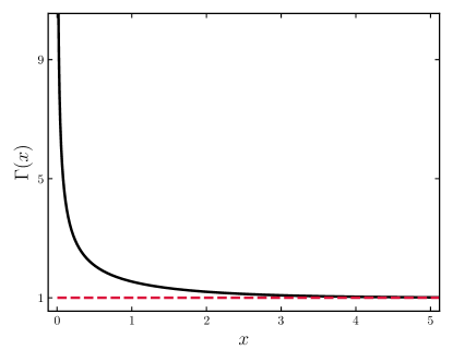
Figure 2: The image of function $\Gamma(x)$; see Eq. (25) with Eq. (20).

As shown in the Fig. 2, when $x\rightarrow\infty$, $\Gamma(x)\rightarrow 1$.

Numerical demonstrations.

As a illustration, we consider a Brownian oscillator system with the Hamiltonian in the Calderia–Leggett form Cal83587 ; Cal83374 ; Wei12 ; Yan05187 ,

$$\begin{split}\hat{H}&=\left(\frac{\hat{p}^{2}}{2m}+\frac{1}{2}m\Omega^{2}\hat{x}^{2}\right)\\ &\quad+\sum_{j}\left[\frac{p_{j}^{2}}{2m_{j}}+\frac{1}{2}m_{j}\omega_{j}^{2}\Big{(}x_{j}-\frac{c_{j}}{m_{j}\omega_{j}^{2}}\hat{x}\Big{)}^{2}\right].\end{split}$$ (26)

It involves a vibrational mode $\hat{x}$ and $\hat{p}$ and its coupling to a solvent bath,

$$h_{\mbox{\tiny B}}=\sum_{j}\Big{(}\frac{p_{j}^{2}}{2m_{j}}+\frac{1}{2}m_{j}\omega_{j}^{2}x_{j}^{2}\Big{)}.$$ (27)

The response of the vibrational mode is defined as

$$\chi(t)\equiv\frac{i}{\hbar}\langle[\hat{x}(t),\hat{x}(0)]\rangle,$$ (28)

where we have denoted

$$\hat{x}(t)\equiv e^{iHt/\hbar}\hat{x}(0)e^{-iHt/\hbar}.$$ (29)

In the frequency domain, its reads Yan05187

$$\begin{split}\tilde{\chi}(\omega)\equiv\int^{\infty}_{0}\!\!{\rm d}t\,e^{i\omega t}\chi(t)=\frac{1/m}{\Omega^{2}-\omega^{2}-i\omega\tilde{\gamma}(\omega)}.\end{split}$$ (30)

Here, the bath–induced friction function is

$$\tilde{\gamma}(\omega)\equiv\int_{0}^{\infty}\!\!{\rm d}t\,e^{i\omega t}\gamma(t)$$ (31)

with

$$\gamma(t)=(1/m)\sum_{j}c_{j}^{2}/(m_{j}\omega_{j}^{2})\cos(\omega_{j}t)$$ (32)

being the classical frictional function. In simulation, we adopt the Drude model for the bath, as

$$\tilde{\gamma}(\omega)=\frac{i\eta\Omega}{\omega+i\zeta}$$ (33)

where $\eta$ and $\zeta$ are two parameters characterizing the coupling strength and damping rate, respectively.

The $C(\omega)$ in Eq. (12) is related to $\tilde{\chi}(\omega)$ via the fluctuation–dissipation theorem reading Cal5134 ; Yan05187

$$C(\omega)=\frac{\hbar\,{\rm Im}\tilde{\chi}(\omega)}{1-e^{-\beta\omega}},$$ (34)

or equivalently [cf. Eq. (15)],

$$c(t)=\frac{\hbar}{\pi}\int_{-\infty}^{\infty}\!\!{\rm d}\omega\,e^{-i\omega t}\frac{{\rm Im}\tilde{\chi}(\omega)}{1-e^{-\beta\omega}}.$$ (35)

From Eq. (35), we can compute the $\Delta x$ and $\Delta p$, and also generator the Boltzmann lower bound. We obtain them numerically at different temperatures and plot the data in Fig. 3.

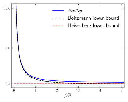
Figure 3: The uncertainty $\Delta x\Delta p$ of the Brownian oscillator system in the Boltzmann states at different temperatures. We set $\hbar=k_{B}=1$, $m=\Omega^{-1}$, and $\tilde{\gamma}(\omega)=i\eta\Omega/(\omega+i\zeta)$ with $\eta=\zeta=10\Omega$.

As shown in Fig. 3, our numerical results support our findings. Besides, we can observe that the Boltzmann lower bound coincides with that of Heisenberg, $\hbar/2$, at extremely low temperatures ($\beta\Omega\gg 1$); see the black versus red dash lines in this regime. This is in line with our physical perception: the thermodynamic effect tapers off when the temperature tends to zero.

Howerver, it is evident that Eq. (3) gives rise to a much more refined lower bound at relatively high temperatures ($\beta\Omega\sim 1$); see the blue solid versus black dash lines. Here, it is the constraint of the thermodynamic canonical distribution that further reduces the precision expressed via the the Heisenberg uncertainty product $\Delta x\Delta p$.

Summary.

To summarize, in this work we investigate the Heisenberg uncertainty product in the context of quantum particles in Boltzmann states. A refined lower bound for this product is derived, which is expressed as a function of the ratio between the standard deviation of position and the thermal de Broglie wavelength. We demonstrate the Boltzmann lower bound on the Brownian oscillator system and compare the results with the traditional Heisenberg uncertainty principle.

Overall, the Boltzmann lower bound represents a new tool for characterizing the thermodynamic precision, and opens up new avenues for future researches in quantum thermodynamics and related fields. It may inspire studies exploring the uncertainty relations in other contexts. For example, exploring the impact of thermal effects on the Heisenberg uncertainty principle may shed light on the complex interactions between quantum mechanics and thermodynamics Lan54643 ; Elc57161 ; Koc81380 ; Mig202471 ; Koy22014104 . From a practical perspective, the refined lower bound developed in this work could be useful in fields such as nanotechnology, where precise measurement of position and momentum is crucial Gar04 ; Cle101155 ; Soa14825 . It could also provide insights into the behavior of complex systems such as biological molecules, where thermal effects are often important Lee071462 ; Che09241 ; Lam1310 . It is anticipated the finding in this work would become an important ingredient in a wide range of fields.

Besides, in a recent analysis based on the thermodynamic considerations, it has been shown that the Heisenberg uncertainty relation is deformed in the quantum gravity regime Buo22136818 . Particularly, the lower bound of the Heisenberg uncertainty product gets increased for positive values of the deformation parameter Buo22136818 . It is attractive to establish relationship between the lower bound deformation with the quantum gravity and that with the thermodynamic considerations presented in this work. This may help understand the gravity–thermodynamic conjecture, originally formulated for black holes in Jac951260 , which establishes a profound connection between gravity and thermodynamic effects.

- (1) W. Heisenberg, The Physical Principles of the Quantum Theory, Courier Corporation, 1949.
- (2) W. Heisenberg, Z. Physik 43, 172 (1927).
- (3) P. Busch, T. Heinonen, and P. Lahti, Phys. Rep. 452, 155 (2007).
- (4) L. Rudnicki, S. P. Walborn, and F. Toscano, Europhys. Lett. 97, 38003 (2012).
- (5) L. A. Rozema, A. Darabi, D. H. Mahler, A. Hayat, Y. Soudagar, and A. M. Steinberg, Phys. Rev. Lett. 109, 100404 (2012).
- (6) H. Bao, S. Jin, J. Duan, S. Jia, K. Mølmer, H. Shen, and Y. Xiao, Nat. Commun. 11, 5658 (2020).
- (7) Y. Hasegawa, Nat. Commun. 14, 2828 (2023).
- (8) S. Lee, C. Hyeon, and J. Jo, Phys. Rev. E 98, 032119 (2018).
- (9) K. Brandner, T. Hanazato, and K. Saito, Phys. Rev. Lett. 120, 090601 (2018).
- (10) Y. Hasegawa and T. Van Vu, Phys. Rev. Lett. 123, 110602 (2019).
- (11) A. M. Timpanaro, G. Guarnieri, J. Goold, and G. T. Landi, Phys. Rev. Lett. 123, 090604 (2019).
- (12) U. Seifert, Physica A 504, 176 (2018).
- (13) Y. Hasegawa and T. Van Vu, Phys. Rev. E 99, 062126 (2019).
- (14) G. Guarnieri, G. T. Landi, S. R. Clark, and J. Goold, Phys. Rev. Res. 1, 033021 (2019).
- (15) J. M. Horowitz and T. R. Gingrich, Nat. Phys. 16, 15 (2020).
- (16) T. Van Vu and K. Saito, Phys. Rev. Lett. 128, 140602 (2022).
- (17) R.-S. Fu and T. R. Gingrich, Phys. Rev. E 106, 024128 (2022).
- (18) T. Kamijima, S. Ito, A. Dechant, and T. Sagawa, Phys. Rev. E 107, L052101 (2023).
- (19) K. Huang, Statistical Mechanics (Second Edition), John Wiley and Sons, New York, 1987.
- (20) D. Chandler, Introduction to Modern Statistical Mechanics, Oxford University Press, New York, 1987.
- (21) P. Strasberg, Quantum Stochastic Thermodynamics: Foundations and Selected Applications, Oxford University Press, 2022.
- (22) Y. J. Yan and R. X. Xu, Annu. Rev. Phys. Chem. 56, 187 (2005).
- (23) H. B. Callen and T. A. Welton, Phys. Rev. 83, 34 (1951).
- (24) J. L. W. V. Jensen, Acta Math. 30, 175 (1906).
- (25) A. O. Caldeira and A. J. Leggett, Physica A 121, 587 (1983).
- (26) A. O. Caldeira and A. J. Leggett, Ann. Phys. 149, 374 (1983), [Erratum: 153, 445 (1984)].
- (27) U. Weiss, Quantum Dissipative Systems, World Scientific, Singapore, 2012, 4rd ed.
- (28) P. T. Landsberg, Phys. Rev. 643, 95 (1954).
- (29) E. W. Elcock and P. T. Landsberg, Phys. Rev. 643, 95 (1954).
- (30) R. H. Koch, D. J. V. Harlingen, and J. Clarke, Appl. Phys. Lett. 38, 380 (1981).
- (31) R. de Miguel and J. M. Rubí, Nanomaterials 10-12, 2471 (2020).
- (32) S. Koyanagi and Y. Tanimura, J. Chem. Phys. 157, 014104 (2022).
- (33) C. W. Gardiner and P. Zoller, Quantum Noise, Springer, Wellington, New Zealand, 2004, 3 ed.
- (34) A. A. Clerk, M. H. Devoret, S. M. Girvin, F. Marquardt, and R. J. Schoelkopf, Rev. Mod. Phys. 82, 1155 (2010).
- (35) A. Soare, H. Ball, D. Hayes, J. Sastrawan, M. C. Jarratt, J. J. McLoughlin, X. Zhen, T. J. Green, and M. J. Biercuk, Nat. Phys. 10, 825 (2014).
- (36) H. Lee, Y.-C. Cheng, and G. R. Fleming, Science 316, 1462 (2007).
- (37) Y. C. Cheng and G. R. Fleming, Annu. Rev. Phys. Chem. 60, 241 (2009).
- (38) N. Lambert, Y.-N. Chen, Y.-C. Cheng, C.-M. Li, G.-Y. Chen, and F. Nori, Nature Physics 9, 10 (2013).
- (39) L. Buoninfante, G. G. Luciano, L. Petruzziello, and F. Scardigli, Phys. Lett. B 824, 136818 (2022).
- (40) T. Jacobson, Phys. Rev. Lett. 75, 1260 (1995).