Q-Learning for Continuous State and Action MDPs under Average Cost Criteria

Abstract

For infinite-horizon average-cost criterion problems, we present several approximation and reinforcement learning results for Markov Decision Processes with standard Borel spaces. Toward this end, (i) we first provide a discretization based approximation method for fully observed Markov Decision Processes (MDPs) with continuous spaces under average cost criteria, and we provide error bounds for the approximations when the dynamics are only weakly continuous under certain ergodicity assumptions. In particular, we relax the total variation condition given in prior work to weak continuity as well as Wasserstein continuity conditions. (ii) We provide synchronous and asynchronous Q-learning algorithms for continuous spaces via quantization, and establish their convergence. (iii) We show that the convergence is to the optimal Q values of the finite approximate models constructed via quantization. Our Q-learning convergence results and their convergence to near optimality are new for continuous spaces, and the proof method is new even for finite spaces, to our knowledge.

1 Introduction

In this paper, we study approximate solutions for Markov decision processes (MDPs) under average cost criteria. We consider problems with continuous state and action spaces and provide approximate planning and reinforcement learning results. We, in particular, show near optimality of the solutions to approximate models and those obtained via reinforcement learning.

Before we present the related research in these problems and discuss our contributions in more detail, we introduce the problem formulation:

A fully observed Markov control model is a five-tuple

$$(\mathbb{X},\mathbb{U},\{\mathbb{U}(x),x\in\mathbb{X}\},{\cal T},c)$$

such that $\mathbb{X}$ is the (standard Borel) state space, $\mathbb{U}$ is the action space, $\mathbb{U}(x)\subset\mathbb{U}$ is the control action set when the state is $x$, so that

$$\mathbb{K}=\{(x,u):x\in\mathbb{X},u\in\mathbb{U}(x)\}\subset\mathbb{X}\times\mathbb{U},$$

is the set of feasible state-action pairs, and ${\cal T}$ is a stochastic kernel on $\mathbb{X}$ given $\mathbb{K}$. Finally $c:\mathbb{K}\to\mathbb{R}$ is the cost function.

Let $\mathbb{H}_{0}:=\mathbb{X},\quad\mathbb{H}_{t}=\mathbb{H}_{t-1}\times\mathbb{K}$ for $t=1,2,\ldots$. We let, for $t\in\mathbb{Z}_{+}$, $h_{t}$ denote an element of $\mathbb{H}_{t}$, where $h_{t}=\{x_{[0,t]},u_{[0,t-1]}\}$, where we use the notation $x_{[0,t]}:=\{x_{0},x_{1},\cdots,x_{t}\}$. An admissible control policy $\gamma$ is a sequence of measurable functions $\{\gamma_{t},t\geq 0\}$ such that $\gamma:\mathbb{H}_{t}\to\mathbb{U}$ with $u_{t}=\gamma_{t}(h_{t})$.

We consider the following average cost problem of finding

$$J^{*}(x):=\inf_{\gamma}J(x,\gamma)=\inf_{\gamma\in\Gamma_{A}}\limsup_{T\to\infty}{1\over T}E^{\gamma}_{x}[\sum_{t=0}^{T-1}c(x_{t},u_{t})]$$ (1)

where $\Gamma_{A}$ is the set of all admissible policies.

1.1 Literature Review

Efficient solutions of MDPs with continuous or finite but large spaces is an important problem. On this, various approximation techniques have been presented, with a partial list including approximate value or policy iteration, approximate dynamic programming, neuro-dynamic programming, reinforcement learning, simulation-based techniques, state aggregation, etc. (see e.g. [9, 3, 7, 4, 39, 40, 36, 26, 11, 38]). Majority of literature have focused on either finite horizon problems and-or infinite horizon discounted cost problems, by using the dynamic programming principle and the contraction properties of Bellman operators via the discount factor. For the average cost problems, however, the same techniques are not immediately applicable.

For MDPs with continuous state spaces, existence for optimal solutions has been well studied under the infinite horizon average cost criteria, under either weak continuity of the kernel (in both the state and action), or strong continuity (of the kernel in actions for every state) properties and measurable selection conditions, together with various stability assumptions. We refer the reader to [2, 14, 16, 17, 8, 12, 41, 42, 16, 5, 10] for comprehensive surveys on optimality results and general solution techniques for optimal control under the average cost criteria. However, research on computational and reinforcement learning methods for average cost optimality still entail open problems, especially for MDPs with continuous spaces.

The contributions of the paper are with regard to finite approximations, their near optimality, and reinforcement learning for average cost problems. We will summarize the related research in these areas separately:

Approximations for the average cost criterion. Related to the aggregation (discretization) methods we will study in this paper, [30, 27, 29, 31] have shown that only under weak continuity conditions for an MDP with standard Borel state and action spaces, finite models obtained by the quantization of the state and action spaces leads to control policies that are asymptotically optimal as the quantization rate increases. However, the aforementioned papers usually focused on the approximation methods under either finite horizon or infinite horizon discounted cost criteria. We note that the analysis of average cost problems is typically more challenging especially for problems with continuous spaces, as the stability (or the ergodicity) of the problem, plays a crucial role. For the average cost criterion, [32], [28, Theorem 4.14] provide error bounds for finite approximations under total variation continuity of the transition models as well as certain mixing conditions.

In our paper, we will relax the total variation continuity condition to weak or Wasserstein continuity.

Reinforcement learning for the average cost criterion.

There are a number of publications that study reinforcement learning methods for MDPs under average cost criterion. To our knowledge, all of these studies focus on finite spaces.

[1, 13] are among the earliest studies that provide convergent learning algorithms based on relative value iteration (as well as stochastic shortest path under a recurrence condition for a given state), and the convergence of these algorithms in these studies have been established via the ODE method [6] for finite models.

Among the relatively more recent studies, [43] provides convergent off-policy learning algorithms without using a reference function/state utilized in [1] (but using an explicit estimate of the reward) to stabilize the value function estimation for finite models; the convergence proof in [43] builds on the ODE method [1, 6]. [47] studies a policy improvement method for average-cost (reward) MDPs for finite state-action spaces. [44] focuses on robust model-free methods for finite systems where the transition model belongs to an uncertainty set which is constructed under various metrics. [37] focuses on relaxing the exponential mixing assumption for average cost criteria for finite models and provides an actor-critic method. Reference [46] studies finite sample guarantees for a synchronous Q-learning algorithm under the average cost criterion. We also note that [45] studies a convergent actor-critic method under average-cost criteria for continuous models with linear systems and additive Gaussian noise. We finally refer the reader to [39] for a general review on the subject primarily under the discounted cost criterion, but also on the average cost criterion.

Almost all of these papers focus on MDP problems under infinite horizon average cost criteria for finite models, i.e. where the state and the actions spaces are finite, and thus are able to use the Markovian nature for learning. The algorithms in the papers noted above possess several variations and impose complementary technical conditions to stabilize the value function updates in the corresponding $Q$-learning algorithms.

[1, Section 5] notes the need for generalizing the analysis to continuous spaces.

Toward this end, in our paper we consider general continuous spaces for which we first construct a discretized model where we present weaker continuity conditions than currently available in the literature. After discretization, the convergence analysis for learning methods requires further adaptations as the discretized states are no longer Markovian. In addition, ergodicity conditions are required to ensure the stability of the associated stochastic iteration algorithms. For continuous models, the ergodicity conditions and the stability analysis differ significantly from those involving finite models. In particular, in our paper, we will obtain an average cost counterpart of the analysis presented in [23], which in turn builds on [22].

Contributions. In view of the above, we address several open questions in the literature along the following directions:

• In Section 3, we provide a discretization based approximation method for fully observed MDPs with continuous spaces under average cost criteria, and we will provide error bounds for the approximations when the dynamics are only weakly continuous under certain ergodicity assumptions. Theorems 7 and 8 present near optimality of control policies obtained for quantized models. Notably, we relax the total variation condition given in [32, 28], where a different technique was utilized, to weak (Feller) continuity (in Theorem 9) or Wasserstein continuity conditions (in Theorems 7 and 8); the former leads only to asymptotic convergence whereas the latter provides a rate of convergence.

• In Section 4, we present quantized Q learning algorithms that will converge to the optimal Q values of the approximate models constructed in Section 3. When one runs the $Q$-learning algorithm, it is important to note that the quantized process is not an MDP, and in fact should be viewed as a POMDP, the view which was utilized in [22] and [23]. In the synchronous setup, however, this does not lead to a challenge as we can simulate the environment under an approximate model, though with an artificial simulation given the data and an off-line analysis. The proof, however, is more direct for this setup. On the other hand, for the asynchronous setup, the data is given sequentially and we cannot rely on Markovian properties. Accordingly, we will generalize the proof method given in [22] for the average cost criterion and we impose ergodicity properties under an exploration policy. In particular, in Section 4.1 we present and study a synchronous Q learning algorithm, and in Section 4.2, we present and study an asynchronous algorithm. Theorem 10 establishes the convergence of a synchronous Q-learning algorithm. Theorem 11 shows the convergence of an asynchronous Q-learning algorithm.

• We finally note that even for the finite space/action setup our Q-learning comvergence proof method is new, to our knowledge; where prior work focused on the ODE method; the proof method presented in our paper facilitates the stochastic analysis needed given the non-Markovian nature of quantized state dynamics.

2 Average Cost Optimality Equation, Contraction Properties of Relative Value Iteration

We start our analysis by first reviewing some related results on average cost optimality.

2.1 The Contraction Properties of Relative Value Iteration

Consider the following average cost problem of finding

$$J^{*}(x):=\inf_{\gamma}J(x,\gamma)=\inf_{\gamma\in\Gamma_{A}}\limsup_{T\to\infty}{1\over T}E^{\gamma}_{x}[\sum_{t=0}^{T-1}c(x_{t},u_{t})]$$ (2)

To study the average cost problem, one common approach is to establish the existence of an Average Cost Optimality Equation (ACOE), and an associated verification theorem.

Definition 1.

The collection of functions $g:\mathbb{X}\to\mathbb{R},h:\mathbb{X}\to\mathbb{R},f:\mathbb{X}\to\mathbb{U}$ is a canonical triplet if for all $x\in\mathbb{X}$,

$$g(x)=\inf_{u\in\mathbb{U}}\int g(x^{\prime}){\cal T}(dx^{\prime}|x,u)$$

$$g(x)+h(x)=\inf_{u\in\mathbb{U}}\bigg{(}c(x,u)+\int h(x^{\prime}){\cal T}(dx^{\prime}|x,u)\bigg{)}$$

with

$$g(x)=\int g(x^{\prime}){\cal T}(dx^{\prime}|x,f(x))$$

$$g(x)+h(x)=\bigg{(}c(x,f(x))+\int h(x^{\prime}){\cal T}(dx^{\prime}|x,f(x))\bigg{)}$$

We will refer to these relations as the Average Cost Optimality Equation (ACOE).

Theorem 2.

[2, 16][Verification Theorem] Let $g,h,f$ be a canonical triplet. a) If $g$ is a constant and

$$\limsup_{n\to\infty}{1\over n}E^{\gamma}_{x}[h(x_{n})]=0,$$ (3)

for all $x$ and under every policy $\gamma$, then the stationary deterministic policy $\gamma^{*}=\{f,f,f,\cdots\}$ is optimal so that

$$g=J(x,\gamma^{*})=\inf_{\gamma\in\Gamma_{A}}J(x,\gamma)$$

where

$$J(x,\gamma)=\limsup_{T\to\infty}{1\over T}E^{\gamma}_{x}[\sum_{k=0}^{T-1}c(x_{t},u_{t})].$$

b) If $g$, considered above, is not a constant and depends on $x$, then under any policy $\gamma$

$$\limsup_{N\to\infty}{1\over N}E_{x}^{\gamma^{*}}[\sum_{t=0}^{N-1}g(x_{t})]\leq\inf_{\gamma}\limsup_{N\to\infty}{1\over N}E^{\gamma}_{x}[\sum_{t=0}^{T-1}c(x_{t},u_{t})],$$

provided that (3) holds. Furthermore, $\gamma^{*}=\{f\}$ is optimal.

2.2 Contraction via the span semi-norm

Fix $z\in\mathbb{X}$ and consider the space of measurable and bounded functions $h$ with the restriction that $h(z)=0$. Let $(g,h,f)$ be a canonical triplet with $g\equiv\rho\in\mathbb{R}$ so that

$$\rho+h(x)=\inf_{u\in\mathbb{U}}\bigg{(}c(x,u)+\int h(x^{\prime}){\cal T}(dx^{\prime}|x,u)\bigg{)}$$

Consider the following assumption.

Assumption 2.1.

For some $\alpha\in[0,1)$, and for all $x,x^{\prime}\in\mathbb{X}$ and $u,u^{\prime}\in\mathbb{U}$

$$\|P(\cdot|x,u)-P(\cdot|x^{\prime},u^{\prime})\|_{TV}\leq 2\alpha$$

Consider the following span semi-norm:

$$\|u\|_{sp}=\sup_{x}u(x)-\inf_{x}u(x)$$

The space of measurable bounded functions that satisfy $h(z)=0$ under the semi-norm $\|u\|_{sp}$ is a Banach space (and hence the semi-norm becomes a norm in this space since $\|u\|_{sp}=0$ implies $u\equiv 0$).

Define

$$\mathbb{T}(h)(x)=\inf_{u\in\mathbb{U}}\bigg{(}c(x,u)+\int h(x^{\prime}){\cal T}(dx^{\prime}|x,u)\bigg{)}$$ (4)

Let

$$(\mathbb{T}_{z}(h))(x)=(\mathbb{T}(h))(x)-(\mathbb{T}(h))(z)$$

Note that $\mathbb{T}_{z}$ maps the aforementioned Banach space to itself under standard measurable selection conditions. see e.g. [16, Theorem 3.3.5].

First note that for pairs $(x,u)$ and $(x^{\prime},u^{\prime})$, with $\mu(dx_{1}):=P(dx_{1}|x,u)-P(dx_{1}|x^{\prime},u^{\prime})$ defining a signed measure, by the Jordan-Hahn decomposition theorem [20, Theorem 2.8] there exists $A$ with $\mu(A)=-\mu(A^{c})\geq 0$ so that the restriction of $\mu$ to $A$ (i.e., $\mu_{A}(B):=\mu(B\cap A)$ for every Borel $B$) defines a non-negative measure and the restriction of $-\mu$ to $A^{c}$ defines a non-negative measure with $\mu(A)-\mu(A^{c})=\|\mu\|_{TV}\leq 2\alpha$ and thus $\mu(A)\leq\alpha$. Thus, for any $x,x^{\prime},u,u;$

$$\int h(x_{1})P(dx_{1}|x,u)-h(x_{1})P(dx_{1}|x^{\prime},u^{\prime})$$

$$=\int_{A}h(x_{1})(P(dx_{1}|x,u)-P(dx_{1}|x^{\prime},u^{\prime}))+\int_{A^{c}}h(x_{1})(P(dx_{1}|x,u)-P(dx_{1}|x^{\prime},u^{\prime}))$$

$$=\int_{A}h(x_{1})(P(dx_{1}|x,u)-P(dx_{1}|x^{\prime},u^{\prime}))-\int_{A^{c}}h(x_{1})(P(dx_{1}|x^{\prime},u^{\prime})-P(dx_{1}|x,u))$$

$$\leq\int_{A}\bigg{(}\sup_{x_{1}}h(x_{1})\bigg{)}(P(dx_{1}|x,u)-P(dx_{1}|x^{\prime},u^{\prime}))-\int_{A^{c}}\bigg{(}\inf_{x_{1}}h(x_{1})\bigg{)}(P(dx_{1}|x^{\prime},u^{\prime})-P(dx_{1}|x,u))$$

$$\leq\bigg{(}\sup_{x_{1}}h(x_{1})\bigg{)}\mu(A)-\bigg{(}\inf_{x_{1}}h(x_{1})\bigg{)}\mu(A^{c})$$

$$\leq\alpha\|h\|_{sp}$$

Then, note that for $v_{1}$ and $v_{2}$ bounded and with $\mathbb{T}(v_{i})(x)$ achieved with control $u^{x}_{i}$ at $x$, we have that for any $x,x^{\prime}$

$$\bigg{(}(\mathbb{T}(v_{1}))(x)-(\mathbb{T}(v_{2}))(x)\bigg{)}-\bigg{(}(\mathbb{T}(v_{1}))(x^{\prime})-(\mathbb{T}(v_{2}))(x^{\prime})\bigg{)}$$

$$\leq\int(v_{1}(x_{1})-v_{2}(x_{1}))\bigg{(}P(dx_{1}|x,u^{x}_{2})-P(dx_{1}|x^{\prime},u^{x^{\prime}}_{1})\bigg{)}\leq\alpha\|v_{1}-v_{2}\|_{sp},$$

(where for the first term $(\mathbb{T}(v_{1}))(x)-(\mathbb{T}(v_{2}))(x)$we upper bound the difference by applying $u^{x}_{2}$ for the right hand side of (4) involving $v_{1}$, and for the second term $(\mathbb{T}(v_{1}))(x^{\prime})-(\mathbb{T}(v_{2}))(x^{\prime})$ we apply $u^{x^{\prime}}_{1}$ for bounding $(\mathbb{T}(v_{2}))(x^{\prime})$) and thus, since $x,x^{\prime}$ are arbitrary, we have

$$\|\mathbb{T}(v_{1})-\mathbb{T}(v_{2})\|_{sp}\leq\alpha\|v_{1}-v_{2}\|_{sp}.$$

Furthermore, since $(\mathbb{T}(v_{i}))(z)$ only serves as a shift term in the following, we have that

$$\|\mathbb{T}_{z}(v_{1})-\mathbb{T}_{z}(v_{2})\|_{sp}=\|\mathbb{T}(v_{1})-\mathbb{T}(v_{2})\|_{sp}\leq\alpha\|v_{1}-v_{2}\|_{sp}.$$

We can then state the following.

Theorem 3.

[14, Lemma 3.5] Under Assumption 2.1, the iterations

$$h_{n+1}=\mathbb{T}_{z}(h_{n}),$$

with $h_{0}\equiv 0$ converges to a fixed point: $\mathbb{T}_{z}(h)=h$, which leads to the ACOE triplet in Definition 1. In particular, if the cost is bounded, under Assumption 2.1, and the controlled kernel satisfies the standard measurable selection conditions, there exists a solution to the ACOE, which in turn leads to an optimal policy.

Remark 2.1.

We recall [15, Theorem 3.2]. The condition in Assumption 2.1 can then be replaced by any of the conditions given in the following:

Proposition 2.1.

[15, Theorem 3.2] Consider the following.

• There exists a state $x^{*}\in\mathbb{X}$ and a number $\beta>0$ such that $\mathcal{T}(\{x^{*}\}|x,\gamma)\geq\beta$, for all $x\in\mathbb{X},\gamma\in\Gamma_{s}$.

• There exists a positive integer $t$ and a non-trivial measure $\mu$ on $\mathbb{X}$ such that $\mathcal{T}^{t}(\cdot|x,\gamma)\geq\mu(\cdot)$ for all $x\in\mathbb{X},\gamma\in\Gamma_{s}$.

• For each $\gamma\in\Gamma_{s}$, the transition kernel $\mathcal{T}(dy|x,\gamma)$ has a density $p(y|x,\gamma)$ with respect to a sigma-finite measure $m$ on $\mathbb{X}$, and there exist $\epsilon>0$ and $C\in\mathcal{B}(\mathbb{X})$ such that $m(C)>0$ and $p(y|x,\gamma)\geq\epsilon$ for all $y\in C,x\in\mathbb{X},\gamma\in\Gamma_{s}$.

• For each $\gamma\in\Gamma_{s}$, $\mathcal{T}(dy|x,\gamma)$ has a density $p(y|x,\gamma)$ with respect to a sigma-finite measure $m$ on $\mathbb{X}$, and $p(y|x,\gamma)\geq p_{0}(y)$ for all $x,y\in\mathbb{X}$, $\gamma\in\Gamma_{s}$, where $p_{0}$ is a non-negative measurable function with $\int p_{0}(y)m(dy)>0$.

• There exists a positive integer $t$ and a measure $\mu$ on $\mathbb{X}$ such that $\mu(\mathbb{X})<2$ and $\mathcal{T}^{t}(\cdot|x,\gamma)\leq\mu(\cdot)$ for all $x\in\mathbb{X},\gamma\in\Gamma_{s}$.

• There exists a positive integer $t$ and a positive number $\beta<1$ such that $\|\mathcal{T}^{t}(\cdot|x,\gamma)-\mathcal{T}^{t}(\cdot|x^{\prime},\gamma)\|_{TV}\leq 2\beta$ for all $x,x^{\prime}\in\mathbb{X},\gamma\in\Gamma_{s}$.

• There exists a positive integer $t$ and a positive number $\beta$ for which the following holds: For each $\gamma\in\Gamma_{s}$, there is a probability measure $\mu_{\gamma}$ on $\mathbb{X}$ such that $\mathcal{T}^{t}(\cdot|x,\gamma)\geq\beta\mu_{\gamma}(\cdot)$ for all $x\in\mathbb{X}$.

• There exist positive numbers $c$ and $\beta$, with $\beta<1$, for which the following holds: For each $\gamma\in\Gamma_{s}$, there is a probability measure $p_{\gamma}$ on $\mathbb{X}$ such that $\|\mathcal{T}^{t}(\cdot|x,\gamma)-p_{\gamma}(\cdot)\|_{TV}\leq c\beta^{t}$ for all $x\in\mathbb{X},t\in\mathds{N}$.

• The state process is uniformly ergodic such that $\lim_{t\to\infty}\|\mathcal{T}^{t}(\cdot|x,\gamma)-p_{\gamma}(\cdot)\|_{TV}=0$ uniformly in $x\in\mathbb{X}$ and $\gamma\in\Gamma_{s}$.

The conditions above are related as follows:

$$a\to b$$

$$e\to f$$

$$c\to d\to b\to f\leftrightarrow g\leftrightarrow h\leftrightarrow i.$$

As a corollary, we conclude that the iteration (4) or $\mathbb{T}_{z}$ is a contraction under any of the conditions in Proposition 2.1 and these can be utilized instead in Theorem 3.

2.3 An alternative argument under the sup norm by equivalence with a discounted cost problem

The following, alternative to the above, approach will prove to be useful in our Q-learning algorithm. We have the following minorization condition.

Assumption 2.2.

There exists a positive measure $\mu$ with

$${\cal T}(B|x,u)\geq\mu(B),$$

for all $B\in{\cal B}(\mathbb{X})$.

Under Assumption 2.2, we have that with

$${\cal T}^{\prime}(\cdot|x,u)={\cal T}(\cdot|x,u)-\mu(\cdot)$$

a positive measure, the map

$$(\mathbb{T}^{\prime}(f))(x)=\min_{u}\bigg{(}c(x,u)+\int f(x_{1}){\cal T}^{\prime}(dx_{1}|x,u)\bigg{)}$$ (5)

is a contraction with contraction constant $\alpha:=1-\mu(\mathds{X})<1$ (see [14, p.61] for a historical review on this approach). With this approach, one avoids the use of the span semi-norm approach. Accordingly, one can apply the standard value iteration algorithm using $(\mathbb{T}^{\prime}$. The limit equation

$$f(x) =\min_{u}(c(x,u)+\int f(x_{1}){\cal T}^{\prime}(dx_{1}|x,u))$$

$$=\min_{u}(c(x,u)+\int f(x_{1}){\cal T}(dx_{1}|x,u))-\int f(x_{1})\mu(dx_{1})$$ (6)

is the desired ACOE in Definition 1 with $g\equiv\int f(x_{1})\mu(dx_{1})$. The existence of a minimizing control policy is ensured under measurable selection conditions, under either weak continuity of the kernel (in both the state and action), or strong continuity (of the kernel in actions for every state) properties and measurable selection conditions. The corresponding measurable selection criteria are given by [18, Theorem 2], [34], [33] and [25]. We also refer the reader to [16] for a comprehensive analysis and detailed literature review.

3 Near Optimality of Quantized State and Action Space Approximations

In the following, we follow [31] [28] to arrive at approximate MDPs with finite state and action spaces. Different from [31] [28], we will require weaker conditions for the average cost criteria (notably, only weak convergence will be sufficient for the average cost approximation results, unlike the total variation continuity assumption in [31] [28]).

Definition 4.

A measurable function $q:{\mathbb{X}}\rightarrow\mathbb{U}$ is called a quantizer from ${\mathbb{X}}$ to $\mathbb{U}$ if the range of $q$, i.e., $q({\mathbb{X}})=\{q(x)\in\mathbb{U}:x\in{\mathbb{X}}\}$, is finite.

The elements of $q({\mathbb{X}})$ (the possible values of $q$) are called the levels of $q$.

3.1 Finite Action Approximate MDP: Quantization of the Action Space

Let $d_{\mathbb{U}}$ denote the metric on $\mathbb{U}$. Since the action space $\mathbb{U}$ is compact and thus totally bounded, one can find a sequence of finite sets $\Lambda_{n}=\{a_{n,1},\ldots,a_{n,k_{n}}\}\subset\mathbb{U}$ such that for all $n$,

$$\min_{i\in\{1,\ldots,k_{n}\}}d_{\mathbb{U}}(a,a_{n,i})<1/n\text{ for all }a\in\mathbb{U}.$$

In other words, $\Lambda_{n}$ is a $1/n$-net in $\mathbb{U}$. Assume that the sequence $\{\Lambda_{n}\}_{n\geq 1}$ is fixed. To ease the notation in the sequel, let us define the mapping

$$\Upsilon_{n}(f)(x):=\mathop{\rm arg\,min}_{a\in\Lambda_{n}}d_{\mathbb{U}}(f(x),a),$$ (7)

where ties are broken so that $\Upsilon_{n}(f)(x)$ is measurable.

We will present conditions on the components of the MDP under which there exists a sequence of finite subsets $\{\Lambda_{n}\}_{n\geq 1}$ of $\mathbb{U}$ for which the following holds:

Assumption 3.1.

• The one stage cost function $c$ is bounded and continuous.

• The stochastic kernel ${\cal T}(\,\cdot\,|x,a)$ is weakly continuous in $(x,a)\in{\mathbb{X}}\times\mathbb{U}$.

• $\mathbb{U}$ is compact.

• $\mathbb{X}$ is compact.

Note that this assumption is essentially a geometric ergodicity condition we studied earlier in Proposition 2.1.

Suppose that Assumptions 3.1 and 2.2 hold. This implies that, as we have seen earlier, there is a solution to the average cost optimality equation (ACOE) and the stationary policy which minimizes this ACOE is an optimal policy.

Theorem 5.

[Average Cost][30, 28] We have, under Assumptions 3.1 and 2.2, the value functions (that is, the optimal expected average cost) satisfy

$$\lim_{n\rightarrow\infty}|V^{*}_{n}-V^{*}|=0,$$

where $V^{*}$ and $V^{*}_{n}$ ($n\geq 1$) (the value functions of the true model and the approximate model sequence, respectively) do not depend on $x$.

One can also obtain rates of convergence results [31] [28], under more stringent Lipschitz continuity conditions.

3.2 Finite State Approximate MDP: Quantization of the State Space

We now establish near optimality under finite state approximations. We construct a finite state MDP building on [31] [28], by choosing a collection of disjoint sets $\{B_{i}\}_{i=1}^{M}$ such that $\bigcup_{i}B_{i}=\mathds{X}$, and $B_{i}\bigcap B_{j}=\emptyset$ for any $i\neq j$. Furthermore, we choose a representative state, $y_{i}\in B_{i}$, for each disjoint set. For this setting, we denote the new finite state space by $\mathds{Y}:=\{y_{1},\dots,y_{M}\}$, and the mapping from the original state space $\mathds{X}$ to the finite set $\mathds{Y}$ is done via

$$q(x)=y_{i}\quad\text{ if }x\in B_{i}.$$ (8)

Furthermore, we choose a weight measure $\pi^{*}\in{\mathcal{P}}(\mathds{X})$ on $\mathds{X}$ such that $\pi^{*}(B_{i})>0$ for all $B_{i}$. We now define normalized measures using the weight measure on each separate quantization bin $B_{i}$ as follows:

$$\hat{\pi}_{y_{i}}^{*}(A):=\frac{\pi^{*}(A)}{\pi^{*}(B_{i})},\quad\forall A\subset B_{i},\quad\forall i\in\{1,\dots,M\},$$ (9)

that is, $\hat{\pi}_{y_{i}}^{*}$ is the normalized weight measure on the set $B_{i}$, where $y_{i}$ belongs to.

We now define the stage-wise cost and transition kernel for the MDP with this finite state space $\mathds{Y}$ using the normalized weight measures. Indeed, for any $y_{i},y_{j}\in\mathds{Y}$ and $u\in\mathds{U}$, the stage-wise cost and the transition kernel for the finite-state model are defined as

$$C^{*}(y_{i},u) =\int_{B_{i}}c(x,u)\,\hat{\pi}_{y_{i}}^{*}(dx),$$

$$P^{*}(y_{j}|y_{i},u) =\int_{B_{i}}\mathcal{T}(B_{j}|x,u)\,\hat{\pi}_{y_{i}}^{*}(dx).$$ (10)

Having defined the finite state space $\mathds{Y}$, the cost function $C^{*}$ and the transition kernel $P^{*}$, we can now introduce the optimal value function for this finite model. We denote the optimal value function which is defined on $\mathds{Y}$ by $\hat{J}:\mathds{Y}\to\mathds{R}$.

Note that we can extend this function over the original state space $\mathds{X}$ by making it constant over the quantization bins. In other words, if $y\in B_{i}$, then for any $x\in B_{i}$, we write

$$\hat{J}(x):=\hat{J}(y).$$

Furthermore, by construction, the extended value function $\hat{J}(x)$ corresponds to the following cost and transition models defined on the original state space $\mathds{X}$:

$$\hat{c}(x,u) =C^{*}(q(x),u)$$

$$\hat{\mathcal{T}}(A|x,u) =\int_{B_{i}}\mathcal{T}(A|x,u)\,\hat{\pi}_{y_{i}}^{*}(dx)\text{ for any }A\in{\mathcal{B}}(\mathds{X}).$$

In the following, we establish approximation and performance results for solutions obtained via the finite MDPs when applied to the true model.

3.3 Finite MDP Approximation via Wasserstein Continuity with Modulus of Continuity in Approximation

We further define an average loss function $L:\mathds{X}\to\mathds{R}$ as a result of the quantization. For some $x\in\mathds{X}$, where $x$ belongs to a quantization bin $B_{i}$ whose representative state is $y_{i}$ (i.e. $q(x)=y_{i}$), a weighted loss function $L(x)$ is defined as

$$L(x):=\int_{B_{i}}\|x-x^{\prime}\|\,\hat{\pi}_{y_{i}}^{*}(dx^{\prime}).$$ (11)

That is, $L(x)$ can be seen as the mean distance to $x$ of the bin $B_{i}$ under the measure $\hat{\pi}^{*}_{y_{i}}$. We denote the uniform bound on the quantization error by $L_{\mathds{X}}$ such that

$$L_{\mathds{X}}:=\sup_{x}L(x)$$

In particular, we have the following immediate result:

Assumption 3.2.

• The original cost function $c$ is Lipschitz, such that $|c(x,u)-c(x^{\prime},u^{\prime})|\leq K_{c}(|x-x^{\prime}|+|u-u^{\prime}|)$ for some $K_{c}<\infty$ for all $x,x^{\prime},u,u^{\prime}$.

• The transition kernel $\mathcal{T}$ is Lipschitz continuous under the first order Wasserstein distance such that $W_{1}(\mathcal{T}(\cdot|x,u),\mathcal{T}(\cdot|x^{\prime},u^{\prime}))\leq K_{f}(|x-x^{\prime}|+|u-u^{\prime}|)$ for some $K_{f}<\infty$ for all $x,x^{\prime},u,u^{\prime}$.

Lemma 6.

Under Assumption 3.2, we have that for all $x,u$

$$|\hat{c}(x,u)-c(x,u)|\leq K_{c}L_{\mathds{X}}$$

$$W_{1}(\hat{\mathcal{T}}(\cdot|x,u),\mathcal{T}(\cdot|x,u))\leq K_{f}L_{\mathds{X}}.$$

Proof.

Let $x\in B_{i}$. For the cost difference, we write

$$|\hat{c}(x,u)-c(x,u)|=\left|\int_{B_{i}}c(x^{\prime},u)\hat{\pi}_{i}^{*}(dx^{\prime})-c(x,u)\right|=\left|\int_{B_{i}}c(x^{\prime},u)-c(x,u)\hat{\pi}_{i}^{*}(dx^{\prime})\right|$$

$$\leq\int_{B_{i}}K_{c}|x-x^{\prime}|\hat{\pi}_{i}^{*}(dx^{\prime})\leq K_{c}L_{\mathds{X}}.$$

For the transition difference, for any $\|f\|_{Lip}\leq 1$, we similarly write

$$\left|\int f(x_{1})\hat{\mathcal{T}}(dx_{1}|x,u)-\int f(x_{1})\mathcal{T}(dx_{1}|x,u)\right|$$

$$=\left|\int\int_{B_{i}}f(x_{1})\mathcal{T}(dx_{1}|x^{\prime},u)\hat{\pi}_{i}^{*}(dx^{\prime})-\int f(x_{1})\mathcal{T}(dx_{1}|x,u)\right|$$

$$\leq\int_{B_{i}}K_{f}|x-x^{\prime}|\hat{\pi}_{i}^{*}(dx^{\prime})\leq K_{f}L_{\mathds{X}}.$$

∎

We impose Assumption 2.2 (the reader can refer to Proposition 2.1 for its relation the ergodicity) on the the kernel $\mathcal{T}$. An immediate implication of Assumption 2.2 is that

$$\hat{\mathcal{T}}(\cdot|x,u)\geq\mu(\cdot)$$

by construction. That is, the discretized MDP also possesses the ergodicity properties of the original MDPS under Assumption 2.2.

Theorem 7.

Under Assumption 3.2 and Assumption 2.2, $J^{*}(x)$ and $\hat{J}(x)$ are constant so that

$$j^{*} =J^{*}(x),\text{ for all }x\in\mathds{X},$$

$$\hat{j} =\hat{J}(x),\text{ for all }x\in\mathds{X}.$$

Furthermore, if $K_{f}<1$

$$|j^{*}-\hat{j}|\leq\frac{K_{c}}{1-K_{f}}L_{\mathds{X}}$$

Proof.

We start by defining the finite horizon problem: Let $J_{T}^{*}(x)$ denote the optimal value function for a finite, $T$, horizon control problem with initial state $x$ for the original problem such that

$$J_{T}^{*}(x)=\inf_{\gamma}\left(\sum_{t=0}^{T}E_{x}^{\gamma}\left[c(X_{t},U_{t})\right]\right).$$

Similarly, we denote the finite horizon value function for the discretized model by $\hat{J}_{T}(x)$. Under Assumption 2.2, for the original model the following ACOE is satisfied for the original model:

$$h(x)=\inf_{u\in\mathds{X}}\left\{c(x,u)+\int h(x_{1})\mathcal{T}(dx_{1}|x,u)\right\}-\int h(x)\mu(dx).$$

Similarly, for the discretized model we have the following ACOE

$$\hat{h}(y)=\inf_{u\in\mathds{X}}\left\{C^{*}(y,u)+\sum\hat{h}(y_{1})P^{*}(y_{1}|y,u)\right\}-\int\hat{h}(q(x))\mu(dx).$$

We then have by Theorem 2:

$$J^{*}(x)=j^{*}=\int h(x)\mu(dx)$$

$$\hat{J}(x)=\hat{j}=\int\hat{h}(q(x))\mu(dx).$$

for all $x\in\mathds{X}$. Furthermore, using the boundedness of the stage-wise cost function, and Assumption 2.2, one can show that the relative value functions $h,\hat{h}$ are uniformly bounded, and thus, it follows that a solution to ACOE exists (by Section 2.3, see also[16, Theorem 5.2.4]) and we have

$$\left|\frac{J_{T}^{*}(x)}{T}-j^{*}\right|\to 0,\qquad\left|\frac{\hat{J}_{T}(x)}{T}-\hat{j}\right|\to 0$$

for all $x\in{\mathds{X}}$, which proves the first part of the result.

For the second part, we write

$$|j^{*}-\hat{j}|\leq\left|J^{*}(x)-\frac{J_{T}^{*}(x)}{T}\right|+\left|\frac{J_{T}^{*}(x)}{T}-\frac{\hat{J}_{T}(x)}{T}\right|+\left|\frac{\hat{J}_{T}(x)}{T}-\hat{J}(x)\right|$$ (12)

In particular, we have that

$$|j^{*}-\hat{j}| \leq\liminf_{T\to\infty}\bigg{(}\left|J^{*}(x)-\frac{J_{T}^{*}(x)}{T}\right|+\left|\frac{J_{T}^{*}(x)}{T}-\frac{\hat{J}_{T}(x)}{T}\right|+\left|\frac{\hat{J}_{T}(x)}{T}-\hat{J}(x)\right|\bigg{)}$$

$$=\lim_{T\to\infty}\left|J^{*}(x)-\frac{J_{T}^{*}(x)}{T}\right|+\liminf_{T\to\infty}\left|\frac{J_{T}^{*}(x)}{T}-\frac{\hat{J}_{T}(x)}{T}\right|+\lim_{T\to\infty}\left|\frac{\hat{J}_{T}(x)}{T}-\hat{J}(x)\right|\bigg{)}$$

since we have that the first and the last terms go to $0$ as $T\to\infty$ (and the limits exist). For the intermediate term, by applying the Abelian inequality, and taking $\beta\uparrow 1$ in [23, Theorem 2.5] (see also [28, Theorem 4.38]), we have that

$$\liminf_{T\to\infty}\left|\frac{J_{T}^{*}(x)}{T}-\frac{\hat{J}_{T}(x)}{T}\right|\leq\frac{K_{c}}{1-K_{f}}L_{\mathds{X}}$$

These lead to the desired result.

∎

The previous result gives us an upper bound on the difference of the value functions, however, it is not practically conclusive, as we are actually interested in the performance of the policy designed for the discretized model when applied for the original model. For this problem, we should note that there be might several policies that achieve the optimal performance for the discretized model under the average cost optimality criterion, and these different policies might perform differently when they are applied to the original problem (see [21, Section 4]).

Hence, we will work with policies that satisfy the ACOE whose existence is guaranteed under Assumption 2.2. In particular, we will find performance loss bounds for the policy $\hat{\gamma}$ that satisfies:

$$\hat{j}+\hat{h}(x) =\hat{c}(x,\hat{\gamma}(x))+\int\hat{h}(x_{1})\hat{\mathcal{T}}(dx_{1}|x,\hat{\gamma}(x))$$ (14)

$$=\inf_{u\in\mathds{U}}\left\{\hat{c}(x,u)+\int\hat{h}(x_{1})\hat{\mathcal{T}}(dx_{1}|x,u)\right\}$$

Theorem 8.

Suppose $\hat{\gamma}$ satisfies (14). Under Assumption 3.2 and Assumption 2.2, if $K_{f}<1$

$$J(x,\hat{\gamma})-J^{*}(x)\leq\frac{2K_{c}}{1-K_{f}}L_{\mathds{X}}$$

Proof.

We start by noting that under Assumption 2.2, we have

$$\mathcal{T}(\cdot|x,u)\geq\mu(\cdot),\qquad\hat{\mathcal{T}}(\cdot|x,u)\geq\mu(\cdot).$$ (15)

In particular, if we define the following operators

$$Th(x):=c(x,\hat{\gamma}(x))+\int h(x_{1})\mathcal{T}(dx_{1}|x,\hat{\gamma}(x))-\int h(x_{1})\mu(dx_{1})$$

$$\hat{T}h(x):=\hat{c}(x,\hat{\gamma}(x))+\int h(x_{1})\hat{\mathcal{T}}(dx_{1}|x,\hat{\gamma}(x))-\int h(x_{1})\mu(dx_{1})$$

$$T^{*}h(x):=c(x,\gamma^{*}(x))+\int h(x_{1})\mathcal{T}(dx_{1}|x,\gamma^{*}(x))-\int h(x_{1})\mu(dx_{1}),$$

where $\gamma^{*}$ is optimal for the average cost problem and solves the ACOE. One can then show that (see (5)), these operators are contractions using the relations (15) with contraction constant $\alpha:=1-\mu(\mathds{X})<1$.

Furthermore, these operators admit unique fixed points, say $h(x),\hat{h}(x),h^{*}(x)$ respectively, such that

$$h(x)=c(x,\hat{\gamma}(x))+\int h(x_{1})\mathcal{T}(dx_{1}|x,\hat{\gamma}(x))-\int h(x_{1})\mu(dx_{1})$$

$$\hat{h}(x)=\hat{c}(x,\hat{\gamma}(x))+\int\hat{h}(x_{1})\hat{\mathcal{T}}(dx_{1}|x,\hat{\gamma}(x))-\int\hat{h}(x_{1})\mu(dx_{1})$$

$$h^{*}(x)=c(x,\gamma^{*}(x))+\int h^{*}(x_{1})\mathcal{T}(dx_{1}|x,\gamma^{*}(x))-\int h^{*}(x_{1})\mu(dx_{1}).$$

Note that the above equations are in the same form as an Average Cost Optimality Equation (ACOE), and hence, we have that $J(x,\hat{\gamma})=\int h(x_{1})\mu(dx_{1})$, $\hat{J}(x)=\int\hat{h}(x_{1})\mu(dx_{1})$, and $J^{*}(x)=\int h^{*}(x_{1})\mu(dx_{1})$.

We now write

$$J(x,\hat{\gamma})-J^{*}(x)\leq\left|J(x,\hat{\gamma})-\hat{J}(x)\right|+\left|\hat{J}(x)-J^{*}(x)\right|.$$

The second term is bounded by Theorem 7. For the first term, we first study the difference $|h(x)-\hat{h}(x)|$:

$$|h(x)-\hat{h}(x)|=|Th(x)-\hat{T}\hat{h}(x)|=|Th(x)-\hat{T}\hat{h}(x)\pm T\hat{h}(x)\pm Th^{*}(x)\pm\hat{T}h^{*}(x)|$$

$$\leq|Th(x)-T\hat{h}(x)|+|T\hat{h}(x)-Th^{*}(x)|+|Th^{*}(x)-\hat{T}h^{*}(x)|+|\hat{T}h^{*}(x)-\hat{T}\hat{h}(x)|$$

$$\leq\alpha\|h-\hat{h}\|_{\infty}+\alpha\|\hat{h}-h^{*}\|_{\infty}+K_{c}L_{\mathds{X}}+\|h^{*}\|_{Lp}K_{f}L_{\mathds{X}}+\alpha\|h^{*}-\hat{h}\|_{\infty}$$

where we have used the fact that the used operators are contractions, and the results of Lemma 6.

We know show that $\|h^{*}\|_{Lip}\leq\frac{K_{c}}{1-K_{f}}$. Note that $\gamma^{*}$ is the optimal policy and also the selector. So, for any $x,x^{\prime}\in\mathds{X}$ we can start by writing

$$|h^{*}(x)-h^{*}(x^{\prime})| \leq\sup_{u}\bigg{|}c(x,u)+\int h^{*}(x_{1})\mathcal{T}(dx_{1}|x,u)-\int h^{*}(x_{1})\mu(dx_{1})$$

$$\qquad\qquad-c(x^{\prime},u)-\int h^{*}(x_{1})\mathcal{T}(dx_{1}|x^{\prime},u)+\int h^{*}(x_{1})\mu(dx_{1})\bigg{|}$$

$$\leq K_{c}|x-x^{\prime}|+K_{f}\|h^{*}\|_{Lip}|x-x^{\prime}|$$

which implies that $\|h^{*}\|_{Lip}\leq\frac{K_{c}}{1-K_{f}}$.

We now focus on the term $\|h^{*}-\hat{h}\|_{\infty}$. Note again that $\hat{\gamma}$ is a selector for the operator $\hat{T}$, as $\gamma^{*}$ is for $T^{*}$, hence we write:

$$|h^{*}(x)-\hat{h}(x)|\leq\sup_{u}\bigg{|} c(x,u)+\int h^{*}(x_{1})\mathcal{T}(dx_{1}|x,u)-\int h^{*}(x_{1})\mu(dx_{1})$$

$$-\hat{c}(x,u)-\int\hat{h}(x_{1})\hat{\mathcal{T}}(dx_{1}|x,u)+\int\hat{h}(x_{1})\mu(dx_{1})\pm\int h^{*}(x_{1})\hat{\mathcal{T}}(dx_{1}|x,u)\bigg{|}$$

$$\leq K_{c}L_{\mathds{X}}+\alpha\|h^{*}-\hat{h}\|_{\infty}+K_{f}L_{\mathds{X}}\|h^{*}\|_{Lip}$$

where we have used Lemma 6 at the last step, and the result that if we denote by the kernel $\hat{\mathcal{T}}^{-}(dx_{1}|x,u):=\hat{\mathcal{T}}(dx_{1}|x,u)-\mu(dx_{1})$, we can write

$$\int h^{*}(x_{1})\hat{\mathcal{T}}(dx_{1}|x,u)-\int\hat{h}(x_{1})\hat{\mathcal{T}}(dx_{1}|x,u)-\int h^{*}(x_{1})\mu(dx_{1})+\int\hat{h}(x_{1})\mu(dx_{1})$$

$$=\int h^{*}(x_{1})\hat{\mathcal{T}}^{-}(dx_{1}|x,u)-\int\hat{h}(x_{1})\hat{\mathcal{T}}^{-}(dx_{1}|x,u)\leq\alpha\|h^{*}-\hat{h}\|_{\infty}$$

We can can rearrange the term and use the bound on $\|h^{*}\|_{Lip}$ to conclude that

$$\|h^{*}-\hat{h}\|_{\infty}\leq\frac{K_{c}}{(1-K_{f})(1-\alpha)}L_{\mathds{X}}.$$

Combining what we have so far, we can write

$$\|h-\hat{h}\|_{\infty}\leq\frac{K_{c}}{(1-K_{f})(1-\alpha)}L_{\mathds{X}}.$$

For the difference $\left|J(x,\hat{\gamma})-\hat{J}(x)\right|$ we then have

$$\left|J(x,\hat{\gamma})-\hat{J}(x)\right|=\left|\int h(x_{1})\mu(dx_{1})-\int\hat{h}(x_{1})\mu(dx_{1})\right|\leq\|h-\hat{h}\|_{\infty}\mu(\mathds{X})$$

$$\leq\frac{K_{c}}{(1-K_{f})(1-\alpha)}L_{\mathds{X}}(1-\alpha)=\frac{K_{c}}{1-K_{f}}L_{\mathds{X}},$$

where we have used the identity $\mu(\mathds{X})=1-\alpha$. Hence, the proof is complete. ∎

3.3.1 Finite Approximations via Weak Continuity and Asymptotic Optimality

We apply a uniform quantization of the compact state space with diameter $\frac{1}{n}$ so that $\sup_{x\in\mathbb{X}}d_{\mathbb{X}}(q(x),x)\leq\frac{1}{n}$.

We recall that in [28, Section 4.2.2] total variation continuity was imposed for near optimality of quantized models under the average cost criterion. In the previous subsection, this was relaxed to Wasserstein continuity. The convergence result along the same lines, can be shown to work under only Assumptions 2.2 and 3.1, as for the intermediate step in (12) weak continuity of the kernel is sufficient. Accordingly, via (5), we present a more relaxed condition, though without a modulus of continuity.

Theorem 9.

Under Assumptions 3.1 and 2.2, we have that

$$\lim_{n\rightarrow\infty}|V^{*}_{n}-V^{*}|=0,$$

Proof.

The proof can build on two alternative approaches. In one, we can consider (12) and for the intermediate term apply the finite horizon analysis via an inductive argument as in [24, Theorem 16] or [31, Theorem 2.2 and 4.1], and for the first and the last terms in (12) utilize uniform ergodicity.

Alternatively, one can apply the contraction analysis on the value iteration given in (5) and directly follow the analysis in [24, Theorem 16]. ∎

Now that we have presented the contraction framework needed for our analysis, we will move on to establishing a Q-learning algorithm and its convergence to near optimality.

4 Quantized Q-Learning for Continuous Spaces under Infinite Horizon Average Cost Criterion

In this section, we will present synchronous and asynchronous Q learning algorithms for systems with continuous spaces and show the convergence to appropriately defined finite MDP models consistent those constructed in Section 3.2.

In the following, we assume that the action space is finite, in view of the approximation discussions in Section 3.1.

We denote by $Q^{*}:\mathds{Y}\times\mathds{U}$ the Q values (factors, or functions) for the finite model introduced in Section 3.2 for some weight measure $\pi^{*}\in{\mathcal{P}}(\mathds{X})$. For any discretized state $y_{i}\in\mathds{Y}$ and any control action $u\in\mathds{U}$, the Q value of the pair $(y_{i},u)$ satisfies the following:

$$j^{*}+Q^{*}(y_{i},u)=C^{*}(y_{i},u)+\sum_{y_{j}\in\mathds{Y}}P^{*}(y_{j}|y_{i},u)\min_{v\in\mathds{U}}Q^{*}(y_{j},v).$$ (16)

where $P^{*}$ and $C^{*}$ are defined in (3.2).

Theorem 7 and Theorem 8 provide bounds on the error of value functions and policies designed for discretized models (and Theorem 9 generalizes this to the case with only weakly continuous models, though with only asymptotic convergence). Hence, if we can find iterations that converge to the Q values in (16), we will be able to obtain performance results through Theorems 7, 8 and 9.

In the following, we present a synchronous and an asynchronous algorithm. When one runs the $Q$-learning algorithm, it is important to note that the quantized process is not an MDP, and in fact should be viewed as a POMDP, the view which was utilized in [22] and [23]. In the synchronous setup, however, this does not lead to a challenge as we can simulate the environment under an approximate model, though with an artificial simulation given the data and an off-line analysis. The proof, however, is more direct for this setup. On the other hand, for the asynchronous setup, the data is given sequentially and we cannot rely on the Markov properties. Accordingly, we will generalize the proof method given in [22] for the average cost criterion and we impose ergodicity properties under an exploration policy.

4.1 Synchronous Q Learning for Discretized Models

We first present a synchronous Q learning algorithm. As noted above, the proof is more direct in this case. In the following, we itemize the synchronous Q-learning algorithm, which we will use in the section. Note that the discretization part of the algorithm follows the same steps as introduced in Section 3.2.

• Choose a collection of disjoint sets $\{B_{i}\}_{i=1}^{M}$ such that $\bigcup_{i}B_{i}=\mathds{X}$, and $B_{i}\bigcap B_{j}=\emptyset$ for any $i\neq j$. Furthermore, choose a representative state, $y_{i}\in B_{i}$, for each disjoint set. Denote the new finite state space by $\mathds{Y}:=\{y_{0},y_{1},\dots,y_{M-1}\}$.

• Pick a discrete state, say $y_{0}$, and an action $u_{0}$ for normalization.

• Define a mapping, $q:\mathds{X}\to\mathds{Y}$ such that

  $$q(x)=y_{i}\quad\text{ if }x\in B_{i}.$$

• Choose a weight measure $\pi^{*}\in{\mathcal{P}}(\mathds{X})$ on $\mathds{X}$ such that $\pi^{*}(B_{i})>0$ for all $B_{i}$. We define normalized measures using the weight measure on each separate quantization bin $B_{i}$ as follows:

  $$\hat{\pi}_{y_{i}}^{*}(A):=\frac{\pi^{*}(A)}{\pi^{*}(B_{i})},\quad\textrm{for Borel $A$}\subset B_{i},\quad\forall i\in\{0,\dots,M-1\}.$$

• Choose a randomized exploration policy $\gamma:\mathds{Y}\to\mathds{U}$

• For the fixed state $y_{0}$, and the action $u_{0}$ generate a state variable, $x_{0}\sim\hat{\pi}_{y_{0}}^{*}(\cdot)$ from the quantization bin $B_{0}$, $y_{0}$ belongs to. Record the cost $C_{0}=c(x_{0},u_{0})$, and the next state $X_{1}^{0}\sim\mathcal{T}(\cdot|x_{0},u_{0})$. Denote by $m_{t}:=C_{0}+\min_{v\in\mathds{U}}Q_{t}(q(X_{1}^{0}),v)$

• At every time step $t$, generate state variables $x_{i}\in B_{i}$ for every $i\in\{0,\dots,M-1\}$ according to the local weight measure $\hat{\pi}_{y_{i}}^{*}$, and pick a control action $u_{i}\in\mathds{U}$ according to the exploration policy $\gamma$. Set $N(y_{i},u_{i})=N(y_{i},u_{i})+1.$

• Observe the cost $C_{i}:=c(x_{i},u_{i})$ and the next state $X_{1}^{i}\sim\mathcal{T}(\cdot|x_{i},u_{i})$ for every $i$.

• Update the Q values synchronously for the control actions assigned at that time step. Note that the iterations are synchronous across the discrete state variables but not across the control actions. For all $i$

  $$Q_{t+1}(y_{i},u_{i})=(1-\alpha_{t}(y_{i},u_{i}))Q_{t}(y_{i},u_{i})+\alpha_{t}(y_{i},u_{i})\left[C_{i}+\min_{v\in\mathds{U}}Q_{t}(q(X_{1}^{i}),v)-m_{t}\right]$$

  where $\alpha_{t}(y_{i},u_{i})=\frac{1}{1+N(y_{i},u_{i})},$

We will study the key step in the algorithm, which is the iteration:

$$Q_{t+1}(y_{i},u_{i})=(1-\alpha_{t}(y_{i},u_{i}))Q_{t}(y_{i},u_{i})+\alpha_{t}(y_{i},u_{i})\left[C_{i}+\min_{v\in\mathds{U}}Q_{t}(q(X_{1}^{i}),v)-m_{t}\right]$$ (17)

where $m_{t}:=C_{0}+\min_{v\in\mathds{U}}Q_{t}(q(X_{1}^{0}),v)$.

Note that even though the algorithm is synchronous for the state variables, the action variables are not updated synchronously, hence, we still keep a different learning rate and a counter for different state-action pairs.

Algorithm 1 Learning Algorithm: Synchronous Quantized Q-Learning

  Input: $Q_{0}$ (initial $Q$-function), $\{B_{i}\}_{i=0}^{M}\subset\mathds{X}$ (quantization bins), $q:\mathds{X}\rightarrow\mathds{Y}$ (quantizer), $\pi^{*}\in{\mathcal{P}}(\mathds{X})$ (weight measure), $\gamma^{*}$ (exploration policy), $L$ (number of iterations), some fixed quantization bin $B_{0}$, $\alpha_{t}$ (learning rates).

  Start with $Q_{0}$

  for $t=0,\ldots,L-1$ do

     

• For the fixed discrete state $y_{0}$ and the action $u_{0}$, generate $x_{0}\in B_{0}$ according to the weight measure $\pi^{*}$, generate the cost $C_{0}=c(x_{0},u_{0})$ and the next state $X^{0}_{1}\sim\mathcal{T}(\,\cdot\,|x_{0},u_{0})$, record $m_{t}=C_{0}+\min_{v\in\mathds{U}}Q_{t}(q(X_{1}^{0}),v)$

     For all $i\in\{0,1,\dots,M\}$

• Generate $x_{i}\in B_{i}$ according to the weight measure $\pi^{*}$, and generate an action $u_{i}$ according to the policy $\gamma$ $\Longrightarrow$ generate the cost $C_{i}=c(x_{i},u_{i})$ and the next state $X^{i}_{t+1}\sim\mathcal{T}(\,\cdot\,|x_{i},u_{i})$, set $N(y_{i},u_{i})=N(y_{i},u_{i})+1.$

• Update $Q$-function $Q_{t}$ for the inputs $(y_{i},u_{i})=(q(x_{i}),u_{i})$ as follows:

  $$Q_{t+1}(y_{i},u_{i})=(1-\alpha_{t}(y_{i},u_{i}))Q_{t}(y_{i},u_{i})+\alpha_{t}(y_{i},u_{i})\left[C_{i}+\min_{v\in\mathds{U}}Q_{t}(q(X_{1}^{i}),v)-m_{t}\right]$$

  where

  $$\alpha_{t}(y_{i},u_{i})=\frac{1}{1+N(y_{i},u_{i})},$$

  end for

  return  $Q_{L}$

The next result show that these iterations converge to the Q values given in (16), for an appropriate weight measure.

Theorem 10.

Under Assumption 2.2, if $\alpha_{t}=\frac{1}{t}$, the iterations given in (17), converge to (16), with

$$j^{*}=\sum_{u\in\mathds{U}}C^{*}(y_{0},u)\gamma(u|y_{0})+\sum_{u\in\mathds{U}}\sum_{y_{j}\in\mathds{Y}}P^{*}(y_{j}|y_{0},u)\min_{v\in\mathds{U}}Q^{*}(y_{j},v)\gamma(u|y_{0}).$$

Furthermore, for any policy $\hat{\gamma}$ such that $Q^{*}(y,\gamma(y))=\min_{u}Q^{*}(y,u)$, under Assumption 3.2, if $K_{f}<1$ we have that

$$J(x,\hat{\gamma})-J^{*}(x)\leq\frac{2K_{c}}{1-K_{f}}L_{\mathds{X}}$$

Proof.

We define the following operator $\mathbb{T}_{0}$ on the bounded measurable functions ${\mathcal{B}}(\mathds{Y}\times{\mathds{U}})$, such that:

$$\mathbb{T}_{0}f(y,u)= C^{*}(y,u)+\sum_{y_{1}}P^{*}(y_{1}|y,u)\min_{v}f(y,v)$$

$$-\sum_{u_{0}}C^{*}(y_{0},u_{0})\gamma(u|y_{0})-\sum_{u_{0}}\sum_{y_{1}}P^{*}(y_{1}|y_{0},u_{0})\min_{v}f(y,v)\gamma(u|y_{0})$$

where the operator depends on the exploration policy $\gamma$. One can show that under Assumption 2.2, the operator is a contraction with $\alpha:=\mu(\mathds{X})<1$.

The fixed point, say $Q^{*}(y,u),$ of the mapping $\mathbb{T}_{0}$, is given by

$$Q^{*}(y,u) =(\mathbb{T}_{0}Q^{*})(y,u)=C^{*}(y,u)+\sum_{y^{\prime}}\min_{u}Q^{*}(y^{\prime},u)P^{*}(y^{\prime}|y,u)-j^{*}$$

where

$$j^{*}=\sum_{u\in\mathds{U}}C^{*}(y_{0},u)\gamma(u|y_{0})+\sum_{u\in\mathds{U}}\sum_{y_{j}\in\mathds{Y}}P^{*}(y_{j}|y_{0},u)\min_{v\in\mathds{U}}Q^{*}(y_{j},v)\gamma(u|y_{0})$$

which satisfies (16).

We claim that the iterations in (17) converge to the fixed point $Q^{*}(y,u)$ for all $(y,u)\in\mathds{Y}\times\mathds{U}$. To show this, let $\Delta_{t}(y_{i},u_{i}):=Q_{t}(y_{i},u_{i})-Q^{*}(y_{i},u_{i})$. We can then write:

$$\Delta_{t}(y_{i},u_{i})=(1-\alpha_{t})Q_{t}(y_{i},u_{i})+\alpha_{t}F_{t}(y_{i},u_{i})$$

where

$$F_{t}(y_{i},u_{i}) =C_{i}+V_{t}(Y_{1}^{i})-C_{0}-V_{t}(Y_{1}^{0})$$

$$-\left[C^{*}(y_{i},u_{i})+\sum_{y_{j}}P^{*}(y_{j}|y_{i},u_{i})V^{*}(y_{j})-\sum_{u_{0}}C^{*}(y_{0},u)\gamma(u_{0}|y_{0})-\sum_{u_{0}}\sum_{y_{j}}P^{*}(y_{j}|y_{0},u_{0})V^{*}(y_{j})\right]$$

where $V_{t}(y):=\min_{v\in\mathds{U}}Q_{t}(y,v)$, and $Y_{1}^{i}=q(X_{1}^{i})$. By [19, Theorem 1], $\Delta_{t}$ converges to 0 uniformly if we can show that

$$E[F_{t}(y_{i},u_{i})]\leq\alpha\|\Delta_{t}\|_{\infty}.$$

We can write

$$E[F_{t}(y_{i},u_{i})] =\int_{B_{i}}c(x,u_{i})\pi_{i}^{*}(dx)+\sum_{y_{j}}V_{t}(y_{j})P^{*}(y_{j}|y_{i},u_{i})$$

$$-\sum_{u_{0}}\int_{B_{0}}c(x,u_{0})\pi_{0}^{*}(dx)\gamma(u_{0}|y_{0})-\sum_{u_{0}}\sum_{y_{j}}V_{t}(y_{j})P^{*}(y_{j}|y_{0},u_{0})\gamma(u_{0}|y_{0})$$

$$-C^{*}(y_{i},u_{i})-\sum_{y_{j}}P^{*}(y_{j}|y_{i},u_{i})V^{*}(y_{j})$$

$$+\sum_{u_{0}}C^{*}(y_{0},u)\gamma(u_{0}|y_{0})+\sum_{u_{0}}\sum_{y_{j}}V^{*}(y_{j})P^{*}(y_{j}|y_{0},u_{0})\gamma(u_{0}|y_{0})$$

$$=\sum_{y_{j}}V_{t}(y_{j})-V^{*}(y_{j})P^{*}(y_{j}|y_{i},u_{i})+\sum_{u_{0}}\sum_{y_{j}}V^{*}(y_{j})-V_{t}(y_{j})P^{*}(y_{j}|y_{0},u_{0})\gamma(u_{0}|y_{0})$$

$$\leq\mathbb{T}_{0}Q_{t}(y_{i},u_{i})-\mathbb{T}_{0}V^{*}(y_{i},u_{i})$$

$$\leq\alpha\|\Delta\|_{\infty}$$

where the last step follows since $\mathbb{T}_{0}$ is a contraction.

For the second part of the result, we note that the limit Q values corresponds to the model introduced in Section 3.2, hence the result follows directly from Theorem 8. ∎

4.2 Asynchronous Q Learning for Discretized Models

The Q-learning algorithm we presented earlier is constructed under the assumption that we can generate samples from every quantization bin synchronously. We now present an algorithm that will learn the Q values and the optimal policy of the finite model constructed in Section 3.2, from a single trajectory.

The decision maker applies an arbitrary admissible policy $\gamma$ and collects realizations of observations, action, and stage-wise cost under this policy:

$$Y_{0},U_{0},c(X_{0},U_{0}),Y_{1},U_{1},c(X_{1},U_{1})\ldots.$$

where $Y_{t}$ denotes the representative state for the quantized state $X_{t}$.

We propose a shifter Q learning algorithm by subtracting the value $\frac{\delta}{|\mathds{Y}|}\sum_{y^{\prime}}V_{t}(y^{\prime})$ for some small enough $\delta>0$, where $V_{t}(y^{\prime})=\min_{u}Q_{t}(y^{\prime},u)$ to get

$$Q_{t+1}(Y_{t},U_{t})=(1-\alpha_{t}(Y_{t},U_{t}))\,Q_{t}(Y_{t},U_{t})$$

$$\phantom{xxxxxxxxxxxxxxxx}+\alpha_{t}(Y_{t},U_{t})\left(c(X_{t},U_{t})+\min_{v\in\mathds{U}}Q_{t}(Y_{t+1},v)-\frac{\delta}{|\mathds{Y}|}\sum_{y^{\prime}}V_{t}(y^{\prime})\right).$$ (18)

The algorithm is summarized as follows:

Algorithm 2 Learning Algorithm: Asynchronous Quantized Q-Learning

  Input: $Q_{0}$ (initial $Q$-function), $q:\mathds{X}\rightarrow\mathds{Y}$ (quantizer), $\gamma^{*}$ (exploration policy), $L$ (number of data points), $\{N(y,u)=0\}_{(y,u)\in\mathds{\mathds{Y}\times\mathds{U}}}$ (number of visits to discrete state-action pairs), $\delta>0$.

  Start with $Q_{0}$

  for $t=0,\ldots,L-1$ do

     

• If $(X_{t},U_{t})$ is the current state-action pair $\Longrightarrow$ observe the cost $c(X_{t},U_{t})$ and the next state $X_{t+1}\sim\mathcal{T}(\,\cdot\,|X_{t},U_{t})$, and set

  $$N(q(X_{t}),U_{t})=N(q(X_{t}),U_{t})+1.$$

• Update $Q$-function $Q_{t}$ for the inputs $(Y_{t},U_{t})=(q(X_{t},U_{t}))$ as follows:

  $$Q_{t+1}(q(X_{t}),U_{t})=(1-\alpha_{t}(q(X_{t}),U_{t}))\,Q_{t}(q(X_{t}),U_{t})$$

  $$\phantom{xxxxxxxxxxxxxxxx}+\alpha_{t}(q(X_{t}),U_{t})\left(c(X_{t},U_{t})+\min_{v\in\mathds{U}}Q_{t}(q(X_{t+1}),v)-\frac{\delta}{|\mathds{Y}|}\sum_{y^{\prime}}V_{t}(y^{\prime})\right),$$

  where

  $$\alpha_{t}(q(X_{t}),U_{t})=\frac{1}{1+N(q(X_{t}),U_{t})},\qquad V_{t}(y)=\min_{u}Q_{t}(y,u).$$

• Generate $U_{t+1}\sim\gamma^{*}(\cdot|q(X_{t+1}))$.

  end for

  return  $Q_{L}$

The following assumptions will be imposed for the convergence.

Assumption 4.1.

• We let $\alpha_{t}(y,u)=0$ unless $(Y_{t},U_{t})=(y,u)$. Otherwise, let

  $$\alpha_{t}(y,u)={1\over 1+\sum_{k=0}^{t}1_{\{Y_{k}=I,U_{k}=u\}}}.$$

• Under the (memoryless or stationary) exploration policy $\gamma(\cdot|\cdot)$, $X_{t}$ is uniquely ergodic and thus has a unique invariant invariant measure $\pi_{\gamma}$.

• During the exploration phase, every observation-action pair $(y,u)$ is visited infinitely often.

We note that a sufficient condition for the second item above is that the state process $\{X_{t}\}_{t\geq 0}$ is positive Harris recurrent under the exploration policy.

We also impose the following assumption on the transitions which is quite similar to Assumption 2.2 with the difference being we now require $\mu(B_{i})>0$ for every quantization bin $B_{i}$. This extra requirement implies that the state may be able to move to any quantization bin under any action with positive probability.

Assumption 4.2.

• There exists a non-trivial measure $\mu(\cdot)$ defined on $\mathds{X}$, with $\mu(\mathds{X})<1$ such that

  $$\mathcal{T}(\cdot|x,u)\geq\mu(\cdot)$$

  for all $x,u\in\mathds{X}\times\mathds{U}$.

• Furthermore, for each quantization bin $B_{i}\subset\mathds{X}$, $\mu(B_{i})>0$.

For the discounted cost criterion, an analogous result was proven in [22] (see also related results in [38] and [35]). It states that the algorithm in (4.1) converges to the optimal Q-function of a MDP whose system components can be described by transition kernel, observation channel, and stage-wise cost of the finite model introduced in Section 3.2.

Theorem 11.

• Under Assumption 4.2 and Assumption 3.2 and Assumption 4.1, the algorithm given in (4.2) converges almost surely, for small enough $\delta$, to $Q^{*}$ which satisfies

  $$j^{*}+Q^{*}(y,u)=C^{*}(y,u)+\sum_{z\in\mathds{Y}}P^{*}(z|y,u)\min_{v\in\mathds{U}}Q^{*}(z,v).$$ (19)

  $P^{*}$ and $C^{*}$ are defined in (3.2) with weight measure being the stationary distribution of the state process $X_{t}$ under the exploration policy.

• Furthermore, for any policy $\hat{\gamma}$ such that $Q^{*}(y,\gamma(y))=\min_{u}Q^{*}(y,u)$, we have that

  $$J(x,\hat{\gamma})-J^{*}(x)\leq\frac{2K_{c}}{1-K_{f}}L_{\mathds{X}}$$

• Under Assumptions 3.1 and 2.2 only, we will have asymptotic convergence.

Proof.

We start by noting that for small enough $\delta$, we have that the positive measure $\mu^{\prime}$ defined as

$$\mu^{\prime}(y^{\prime})=\frac{\delta}{|\mathds{Y}|}$$

satisfies

$$P^{*}(\cdot|y,u)\geq\mu(\cdot)\geq\mu^{\prime}(\cdot).$$

We now define the following new transition measure (not necessarily a conditional probability measure)

$$\hat{P}^{*}(\cdot|y,u)=P^{*}(\cdot|y,u)-\mu^{\prime}(\cdot).$$

Then, as noted earlier, the following operator is a contraction with $1-\delta$ on bounded measurable functions ${\mathcal{B}}(\mathds{Y}\times{\mathds{U}})$ (see (5) and [14, p.61])

$$(\hat{\mathbb{T}}f)(y,u)=C^{*}(y,u)+\sum_{y^{\prime}}\min_{u}f(y^{\prime},u)\hat{P}^{*}(y^{\prime}|y,u).$$

We define the fixed point, say $Q^{*}(y,u),$ of the mapping $\hat{\mathbb{T}}$, such that

$$Q^{*}(y,u) =(\hat{\mathbb{T}}Q^{*})(y,u)=C^{*}(y,u)+\sum_{y^{\prime}}\min_{u}Q^{*}(y^{\prime},u)\hat{P}^{*}(y^{\prime}|y,u)$$

$$=C^{*}(y,u)+\sum_{y^{\prime}}\min_{u}Q^{*}(y^{\prime},u)P^{*}(y^{\prime}|y,u)-\sum_{y^{\prime}}\min_{u}Q^{*}(y^{\prime},u)\mu^{\prime}(y^{\prime})$$

$$=C^{*}(y,u)+\sum_{y^{\prime}}\min_{u}Q^{*}(y^{\prime},u)P^{*}(y^{\prime}|y,u)-\frac{\delta}{|\mathds{Y}|}\sum_{y^{\prime}}\min_{u}Q^{*}(y^{\prime},u)$$

which satisfies an ACOE with $\frac{\delta}{|\mathds{Y}|}\sum_{y^{\prime}}\min_{u}Q^{*}(y^{\prime},u)=j^{*}$.

We claim that the iterations converge to $Q^{*}$. Now, let $\Delta(y_{i},u_{i}):=Q_{t}(y_{i},u_{i})-Q^{*}(y_{i},u_{i})$, we then write

$$\Delta_{t+1}(y_{i},u_{i})=(1-\alpha_{t}(y_{i},u_{i}))\Delta_{t}(y_{i},u_{i})+\alpha_{t}(y_{i},u_{i})F_{t}(y_{i},u_{i})$$

where

$$F_{t}(y_{i},u_{i})= \left(C_{i}+V_{t}(Y_{t+1})-\frac{\delta}{|\mathds{Y}|}\sum_{y^{\prime}}V_{t}(y^{\prime})\right)$$

$$-\left(C^{*}(y_{i},u_{i})+\sum_{y^{\prime}}V^{*}(y^{\prime})P^{*}(y^{\prime}|y,u)-\frac{\delta}{|\mathds{Y}|}\sum_{y^{\prime}}V^{*}(y^{\prime})\right)$$

where $Y_{t+1}=q(X_{t+1})$. We now write $F_{t}=\hat{F}_{t}+r_{t}$ by adding and subtracting $V^{*}(Y_{t+1})$ where

$$\hat{F}_{t}(y_{i},u_{i})=V_{t}(Y_{t+1})-\frac{\delta}{|\mathds{Y}|}\sum_{y^{\prime}}V_{t}(y^{\prime})-\left(V^{*}(Y_{t+1})-\frac{\delta}{|\mathds{Y}|}\sum_{y^{\prime}}V^{*}(y^{\prime})\right)$$

$$r_{t}(y_{i},u_{i})=C_{i}-C^{*}(y_{i},u_{i})+V^{*}(Y_{t+1})-\frac{\delta}{|\mathds{Y}|}\sum_{y^{\prime}}V^{*}(y^{\prime}).$$

We further separate

$$\hat{F}_{t}(y_{i},u_{i})=E[\hat{F}_{t}(y_{i},u_{i})|h_{t}]+\left(\hat{F}_{t}(y_{i},u_{i})-E[\hat{F}_{t}(y_{i},u_{i})|h_{t}]\right)$$

where $h_{t}=\{y_{t},u_{t},\dots,y_{0},u_{0}\}$. We define three processes $\delta_{t}(y_{i},u_{i})$, $w_{t}(y_{i},u_{i})$, and $v_{t}(y_{i},u_{i})$:

$$\delta_{t+1}(y_{i},u_{i})=(1-\alpha_{t}(y_{i},u_{i}))\delta_{t}(y_{i},u_{i})+\alpha_{t}(y_{i},u_{i})E[\hat{F}_{t}(y_{i},u_{i})|h_{t}]$$

$$w_{t+1}(y_{i},u_{i})=(1-\alpha_{t}(y_{i},u_{i}))w_{t}(y_{i},u_{i})+\alpha_{t}(y_{i},u_{i})\left(\hat{F}_{t}(y_{i},u_{i})-E[\hat{F}_{t}(y_{i},u_{i})|h_{t}]\right)$$

$$v_{t+1}(y_{i},u_{i})=(1-\alpha_{t}(y_{i},u_{i}))v_{t}(y_{i},u_{i})+\alpha_{t}(y_{i},u_{i})r_{t}(y_{i},u_{i}).$$

We first show that $v_{t}(y_{i},u_{i})\to 0$ for all $(y_{i},u_{i})$. Since the learning rates are linear, one can show that $v_{t}\to 0$, if

$$\frac{1}{T}\sum_{t=1}^{T}C_{i}\to C^{*}(y_{i},u_{i})$$

$$\frac{1}{T}\sum_{t=1}^{T}V^{*}(Y_{t+1}^{i})\to\sum_{y^{\prime}}V^{*}(y^{\prime})P^{*}(y^{\prime}|y_{i},u_{i})$$

where $Y_{t+1}^{i}$ denotes the next quantized state following the pair $(y_{i},u_{i})$ after the $t$th time $(t_{i},u_{i})$ have been visited. Both these convergences holds since we assume that the controlled state process $X_{t}$ converges to its unique invariant measure, $\pi_{\gamma}$ under the exploration policy $\gamma$.

The process $v_{t}(y_{i},u_{i})$ converges to 0 since $E\left(\hat{F}_{t}(y_{i},u_{i})-E[\hat{F}_{t}(y_{i},u_{i})|h_{t}]\right)=0$.

Note that under Assumption 4.2

$$E[\hat{F}_{t}(y_{i},u_{i})|h_{t}]\leq\alpha\|V_{t}-V^{*}\|_{\infty}\leq\alpha\|\Delta_{t}\|_{\infty}$$

where $\alpha:=(1-\delta)<1$.

Since, we have that $(w_{t}+v_{t})(y_{i},u_{i})\to 0$ for all $(y_{i},u_{i})$, and $E[\hat{F}_{t}(y_{i},u_{i})|h_{t}]\leq\alpha\|\Delta_{t}\|_{\infty}$; for $\Delta_{t}=\delta_{t}+w_{t}+v_{t}$, for $t>T$ such that $\|w_{t}+v_{t}\|_{\infty}\leq\epsilon$ we can write

$$\Delta_{t}(y_{i},u_{i})\leq(1-\alpha_{t}(y_{i},u_{i}))\Delta_{t}(y_{i},u_{i})+\alpha_{t}(y_{i},u_{i})\alpha(\|\Delta\|_{\infty}+\epsilon)$$ (20)

Hence, following the proof of [22, Theorem 4.1], we can show that $\|\Delta_{t}\|_{\infty}\to 0$. In particular, one can choose some $C<\infty$, such that $\hat{\alpha}:=\alpha(C+1)/C<1$, so that

$$\alpha(\|\Delta\|_{\infty}+\epsilon)\leq\hat{\alpha}\|\Delta\|_{\infty}.$$

For $\|\Delta\|_{\infty}>C\epsilon$, we can rearrange (20), to show that

$$\Delta_{t}(y_{i},u_{i})<\|\Delta\|_{\infty},$$

which implies that for $\|\Delta\|_{\infty}>C\epsilon$ the process monotonically decreases. Then, there are two possibilities: it either gets below $C\epsilon$ or it never gets below $C\epsilon$ in which case by the monotone non-decreasing property it will converge to some number, say $M_{1}$ with $M_{1}\geq C\epsilon$.

If $\|\Delta\|_{\infty}$ ever gets below $C\epsilon$ , by rearranging (20), we can also show that

$$\Delta_{t}(y_{i},u_{i})<C\epsilon$$

hence it always stays below $C\epsilon$. Following the steps in the proof of [22, Theorem 4.1], we can also show that it is not possible that $M_{1}\geq C\epsilon$, which proves item $(i)$.

(ii) and (iii) are consequences of Theorems 7, 8 and 9.

∎

Remark 4.1.

One further difference between the synchronous and the asynchronous Q-learning algorithms presented is that in the latter, Assumption 4.2(ii) holds and a lower bound (represented by $\frac{\delta}{|\mathbb{Y}|}$ in the algorithm) is assumed to be known, whereas in the former this condition (and therefore its knowledge) is not assumed; on the other hand, the synchronous algorithm is not on-line.

5 Simulation and Case Study

We consider a variant of the machine replacement problem adapted to continuous spaces. We let the state space to be $\mathds{X}=[0,1]$, and the action space to be $\mathds{U}=[-1,1]$. The state $x$ represents how well the machine operates where $0$ represents a fully broken machine, and the state $1$ represents a fully functioning machine. The control action $u$ represents the repair effort, where $u=0$ means no repair at all, and $u=1$ means full effort for the repair. The stage wise cost function is given by

$$c(x,u)=0.7(1-x)+0.2(u+1)$$

For the dynamics we assume; if $u>0$, for a given state $x$

$$x_{1}\sim\begin{cases}&\rm{Unif}[x,\min(x+u,1)]\text{ w.p. }0.9\\ &\rm{Unif}[0,1]\text{ w.p. }0.1\end{cases}$$

i.e. the repair moves to state towards $1$ randomly if it works with probability 0.9 or the state is moved somewhere in $[0,1]$ uniformly with probability $0.1$ if the repair does not work.

If $u\leq 0$

$$x_{1}\sim\begin{cases}&\rm{Unif}[\max(x+u,0),x]\text{ w.p. }0.9\\ &\rm{Unif}[0,1]\text{ w.p. }0.1\end{cases}$$

i.e. either the state is moved towards state $0$ uniformly with probability 0.9 or it is moved somewhere in $[0,1]$ uniformly with probability $0.1$.

The following Figure 1 is for the relative value function convergence of the synchronous and the asynchronous algorithms when we use the discretized state space and action with size 5. Recall that the relative value function that satisfies the ACOE is not unique and any shifted version of the function satisfies the ACOE. Hence, for better comparison we normalize them by subtracting the minimum value the functions when we plot them. It can be seen that there is slight difference between the limit values for asynchronous and synchronous algorithms. The reason is that the weight measure $\pi^{*}$ (see (9)) is different for both algorithms. For the asynchronous algorithm, $\pi^{*}$ is the invariant measure of the state process under the exploration policy, whereas for the synchronous one, $\pi^{*}$ depends on our choice to generate the states. In particular, for the plotted values, we have used the uniform measure.

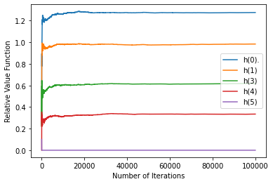
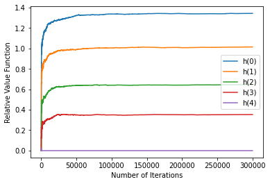
Fig. 1: Relative value function convergence for synchronous(left) and asynchronous(right) algorithms

The following Figure 2 shows the convergence of the value constant, i.e. $\frac{\delta}{\mathds{Y}}\sum_{y^{\prime}}V_{t}(y^{\prime})$, for different initial values $x_{0}=0.3,0.5,0.8$ for the asynchronous algorithm. We use the discretized action values $\hat{\mathds{U}}=\{-1,0,1\}$, and for the state space we choose the bins to be the intervals $[0,0.25],(0.25,0.5],(0.5,0.75],(0.75,1]$. As it can be seen from the figure, and as expected, the limit value constant does not depend on the initial state.

Fig. 2: Algorithm convergence under different initial conditions

In Figure 3, the above line shows the total average cost when we use the policy learned by the algorithm when we use $\hat{\mathds{U}}=\{-1,0,1\}$ for different quantization rates in the state space, and the below line shows the performances of the learned policies when $\hat{\mathds{U}}=\{-1,-0.5,0,0.5,1\}$ for different state space quantization. For the state space, we use uniform quantization, i.e. if the size of the discrete state space is $M=3$, the quantization bins are $[0,\frac{1}{3}],(\frac{1}{3},\frac{2}{3}],(\frac{2}{3},1]$. It is clear from the figure that as the quantization rate increases the regret decreases. Note that the asynchronous and the synchronous algorithms learn the same policy, therefore we do not plot them separately.

Fig. 3: Learned policy performance under different quantization rates

6 Concluding Remarks

For infinite-horizon average-cost criterion problems, we presented approximation and reinforcement learning results for Markov Decision Processes with standard Borel spaces. We first provided a discretization based approximation method for fully observed Markov Decision Processes (MDPs) with continuous spaces under average cost criteria, and we provide error bounds for the approximations when the dynamics are only weakly continuous under certain ergodicity assumptions. In particular, we relaxed the total variation condition given in prior work to weak continuity as well as Wasserstein continuity conditions. We then presented synchronous and asynchronous Q-learning algorithms for continuous spaces via quantization, and establish their convergence. We showed that the convergence is to the optimal Q values of the finite approximate models constructed via quantization.

A future research problem is the following. Since we are considering an average cost problem, one can obtain an online Q-learning algorithm where the past is used to optimally adapt the exploration policy, so that the optimal cost is obtained for each sample path under mild ergodicity conditions. This can be done, e.g. by increasing the exploration lengths and adapting the obtained policy with a diminishing exploration.

References

- [1] J. Abounadi, D. Bertsekas, and V. S. Borkar. Learning algorithms for Markov decision processes with average cost. SIAM Journal on Control and Optimization, 40(3):681–698, 2001.
- [2] A. Arapostathis, V. S. Borkar, E. Fernandez-Gaucherand, M. K. Ghosh, and S. I. Marcus. Discrete-time controlled Markov processes with average cost criterion: A survey. SIAM J. Control and Optimization, 31:282–344, 1993.
- [3] D.P. Bertsekas. Convergence of discretization procedures in dynamic programming. IEEE Trans. Autom. Control, 20(3):415–419, Jun. 1975.
- [4] D.P. Bertsekas and J.N. Tsitsiklis. Neuro-dynamic programming. Athena Scientific, 1996.
- [5] V. S. Borkar. Convex analytic methods in Markov decision processes. In Handbook of Markov Decision Processes, E. A. Feinberg, A. Shwartz (Eds.), pages 347–375. Kluwer, Boston, MA, 2001.
- [6] V.S. Borkar and S.P. Meyn. The ode method for convergence of stochastic approximation and reinforcement learning. SIAM Journal on Control and Optimization, 38(2):447–469, 2000.
- [7] C.S. Chow and J. N. Tsitsiklis. An optimal one-way multigrid algorithm for discrete-time stochastic control. IEEE transactions on automatic control, 36(8):898–914, 1991.
- [8] O. Costa and F. Dufour. Average control of markov decision processes with feller transition probabilities and general action spaces. Journal of Mathematical Analysis and Applications, 396(1):58–69, 2012.
- [9] F. Dufour and T. Prieto-Rumeau. Approximation of Markov decision processes with general state space. J. Math. Anal. Appl., 388:1254–1267, 2012.
- [10] E.A. Feinberg, P.O. Kasyanov, and N.V. Zadioanchuk. Average cost Markov decision processes with weakly continuous transition probabilities. Math. Oper. Res., 37(4):591–607, Nov. 2012.
- [11] C. Gaskett and A. Zelinsky D. Wettergreen. Q-learning in continuous state and action spaces. In Australasian joint conference on artificial intelligence, pages 417–428. Springer, 1999.
- [12] E. Gordienko and O. Hernandez-Lerma. Average cost Markov control processes with weighted norms: Existence of canonical policies. Appl. Math., 23(2):199–218, 1995.
- [13] Abhijit Gosavi. Reinforcement learning for long-run average cost. European journal of operational research, 155(3):654–674, 2004.
- [14] O. Hernandez-Lerma. Adaptive Markov control processes, volume 79. Springer Science & Business Media, 2012.
- [15] O. Hernández-Lerma, R. Montes de Oca, and R. Cavazos-Cadena. Recurrence conditions for markov decision processes with borel state space: a survey. Annals of Operations Research, 28(1):29–46, 1991.
- [16] O. Hernandez-Lerma and J. B. Lasserre. Discrete-Time Markov Control Processes: Basic Optimality Criteria. Springer, 1996.
- [17] O. Hernández-Lerma and J. B. Lasserre. Further topics on discrete-time Markov control processes. Springer, 1999.
- [18] C. J. Himmelberg, T. Parthasarathy, and F. S. Van Vleck. Optimal plans for dynamic programming problems. Mathematics of Operations Research, 1(4):390–394, 1976.
- [19] T. Jaakkola, M. I. Jordan, and S. P. Singh. On the convergence of stochastic iterative dynamic programming algorithms. Neural computation, 6(6):1185–1201, 1994.
- [20] O. Kallenberg. Foundations of Modern Probability. Springer-Verlag, New York, 1997.
- [21] A. D. Kara, M. Raginsky, and S. Yüksel. Robustness to incorrect models and data-driven learning in average-cost optimal stochastic control. Automatica, 139:110179, 2022.
- [22] A. D. Kara and S. Yüksel. Convergence of finite memory Q learning for POMDPs and near optimality of learned policies under filter stability. Mathematics of Operations Research, 2022.
- [23] A.D Kara, N. Saldi, and S. Yüksel. Q-learning for MDPs with general spaces: Convergence and near optimality via quantization under weak continuity. Journal of Machine Learning Research, 2023 (arXiv:2111.06781), 2023.
- [24] Ali D. Kara and S. Yüksel. Robustness to approximations and model learning in mdps and pomdps. In A. B. Piunovskiy and Y. Zhang, editors, Modern Trends in Controlled Stochastic Processes: Theory and Applications, Volume III. Luniver Press, 2021.
- [25] K. Kuratowski and C. Ryll-Nardzewski. A general theorem on selectors. Bull. Acad. Polon. Sci. Ser. Sci. Math. Astronom. Phys, 13(1):397–403, 1965.
- [26] F. C. Melo, S. P. Meyn, and I. M. Ribeiro. An analysis of reinforcement learning with function approximation. In Proceedings of the 25th international conference on Machine learning, pages 664–671, 2008.
- [27] N. Saldi, T. Linder, and S. Yüksel. Asymptotic optimality and rates of convergence of quantized stationary policies in stochastic control. IEEE Trans. Automatic Control, 60:553 –558, 2015.
- [28] N. Saldi, T. Linder, and S. Yüksel. Finite Approximations in Discrete-Time Stochastic Control: Quantized Models and Asymptotic Optimality. Springer, Cham, 2018.
- [29] N. Saldi, S. Yüksel, and T. Linder. Finite-state approximation of Markov decision processes with unbounded costs and Borel spaces. In IEEE Conf. Decision Control, Osaka. Japan, December 2015.
- [30] N. Saldi, S. Yüksel, and T. Linder. Near optimality of quantized policies in stochastic control under weak continuity conditions. Journal of Mathematical Analysis and Applications, also arXiv:1410.6985, 2015.
- [31] N. Saldi, S. Yüksel, and T. Linder. On the asymptotic optimality of finite approximations to markov decision processes with borel spaces. Mathematics of Operations Research, 42(4):945–978, 2017.
- [32] Naci Saldi. Finite-state approximations to discounted and average cost constrained markov decision processes. IEEE Transactions on Automatic Control, 64(7):2681–2696, 2019.
- [33] M. Schäl. A selection theorem for optimization problems. Archiv der Mathematik, 25(1):219–224, 1974.
- [34] M. Schäl. Conditions for optimality in dynamic programming and for the limit of n-stage optimal policies to be optimal. Z. Wahrscheinlichkeitsth, 32:179–296, 1975.
- [35] S. P. Singh, T. Jaakkola, and M. I. Jordan. Learning without state-estimation in partially observable markovian decision processes. Machine Learning Proceedings 1994, pages 284–292, 1994.
- [36] S. P. Singh, T. Jaakkola, and M. I. Jordan. Reinforcement learning with soft state aggregation. Advances in neural information processing systems, pages 361–368, 1995.
- [37] W. A. Suttle, A. Bedi, B. Patel, B. M. Sadler, A. Koppel, and D. Manocha. Beyond exponentially fast mixing in average-reward reinforcement learning via multi-level Monte Carlo actor-critic. In Proceedings of the 40th International Conference on Machine Learning, volume 202 of Proceedings of Machine Learning Research, pages 33240–33267. PMLR, 23–29 Jul 2023.
- [38] C. Szepesvári and W. D. Smart. Interpolation-based q-learning. In Proceedings of the twenty-first international conference on Machine learning, page 100, 2004.
- [39] C. Szepesvári. Algorithms for reinforcement learning. volume 4, pages 1–103, 2010.
- [40] J. N. Tsitsiklis and B. Van Roy. An analysis of temporal-difference learning with function approximation. IEEE transactions on automatic control, 42(5):674–690, 1997.
- [41] O. Vega-Amaya. The average cost optimality equation: a fixed point approach. Bol. Soc. Mat. Mexicana, 9(3):185–195, 2003.
- [42] Oscar Vega-Amaya. The average cost optimality equation: a fixed point approach. Bol. Soc. Mat. Mexicana, 9(1):185–195, 2003.
- [43] Y. Wan, A. Naik, and R. S. Sutton. Learning and planning in average-reward Markov decision processes. In International Conference on Machine Learning, pages 10653–10662. PMLR, 2021.
- [44] Y. Wang, A. Velasquez, G. K. Atia, A. Prater-Bennette, and S. Zou. Model-free robust average-reward reinforcement learning. In Proceedings of the 40th International Conference on Machine Learning, volume 202 of Proceedings of Machine Learning Research, pages 36431–36469. PMLR, 23–29 Jul 2023.
- [45] Z. Yang, Y. Chen, M. Hong, and Z. Wang. Provably global convergence of actor-critic: A case for linear quadratic regulator with ergodic cost. Advances in neural information processing systems, 32, 2019.
- [46] S. Zhang, Z. Zhang, and S.T. Maguluri. Finite sample analysis of average-reward td learning and -learning. Advances in Neural Information Processing Systems, 34:1230–1242, 2021.
- [47] Y. Zhang and K. W. Ross. On-policy deep reinforcement learning for the average-reward criterion. In Marina Meila and Tong Zhang, editors, Proceedings of the 38th International Conference on Machine Learning, volume 139 of Proceedings of Machine Learning Research, pages 12535–12545. PMLR, 18–24 Jul 2021.