ST-MLP: A Cascaded Spatio-Temporal Linear Framework with Channel-Independence Strategy for Traffic Forecasting

Abstract

The criticality of prompt and precise traffic forecasting in optimising traffic flow management in Intelligent Transportation Systems (ITS) has drawn substantial scholarly focus. Spatio-Temporal Graph Neural Networks (STGNNs) have been lauded for their adaptability to road graph structures. Yet, current research on STGNNs architectures often prioritises complex designs, leading to elevated computational burdens with only minor enhancements in accuracy. To address this issue, we propose ST-MLP, a concise spatio-temporal model solely based on cascaded Multi-Layer Perceptron (MLP) modules and linear layers. Specifically, we incorporate temporal information, spatial information and predefined graph structure with a successful implementation of the channel-independence strategy - an effective technique in time series forecasting. Empirical results demonstrate that ST-MLP outperforms state-of-the-art STGNNs and other models in terms of accuracy and computational efficiency. Our finding encourages further exploration of more concise and effective neural network architectures in the field of traffic forecasting.

Introduction

Traffic forecasting is pivotal in the Intelligent Traffic System (ITS) since it can provide accurate road status data that aids informed decision-making for agencies (Wang et al. 2023b; Wang, Sun, and Boukerche 2022; Wang et al. 2022a). Consequently, it has gained considerable attention from both academia and industry (Wang et al. 2023a, 2022b).

Traffic forecasting is often treated as a spatio-temporal time series forecasting problem (Jin et al. 2023). Thanks to the rise of deep learning, spatio-temporal graph neural networks (STGNNs) have become a popular research direction. Various STGNNs have been introduced, showing impressive forecasting accuracy (Weng et al. 2023; Guo et al. 2021, 2019). These models use different strategies: some rely on predefined adjacency matrices to capture spatial correlations (Guo et al. 2019; Wu et al. 2019), while others use neural networks to extract dynamic spatial patterns (Guo et al. 2021; Bai et al. 2020; Oreshkin et al. 2021). A few even combine both methods (Shao et al. 2022b). However, recent STGNNs have grown more complex without delivering much better performance, leading to longer computation times and higher memory usage (Shao et al. 2022a). This situation has prompted a reevaluation of these complex architectures, sparking a search for simpler and more efficient techniques (Liu et al. 2023a).

In time series forecasting, some simpler yet effective methods like TSMixer (Ekambaram et al. 2023) and TiDE (Das et al. 2023) have shown strong performance on different forecasting tasks. In the area of analyzing spatio-temporal data, a straightforward approach called STID by Shao et al. combines spatial and temporal information using MLPs, achieving good results while being efficient (Shao et al. 2022a). Also, Qin et al. designed an architecture based on MLP transformers (Qin et al. 2023) that outperforms many complex models. Yet, despite these successful examples, there’s still a lack of exploration of concise models in traffic and spatio-temporal forecasting.

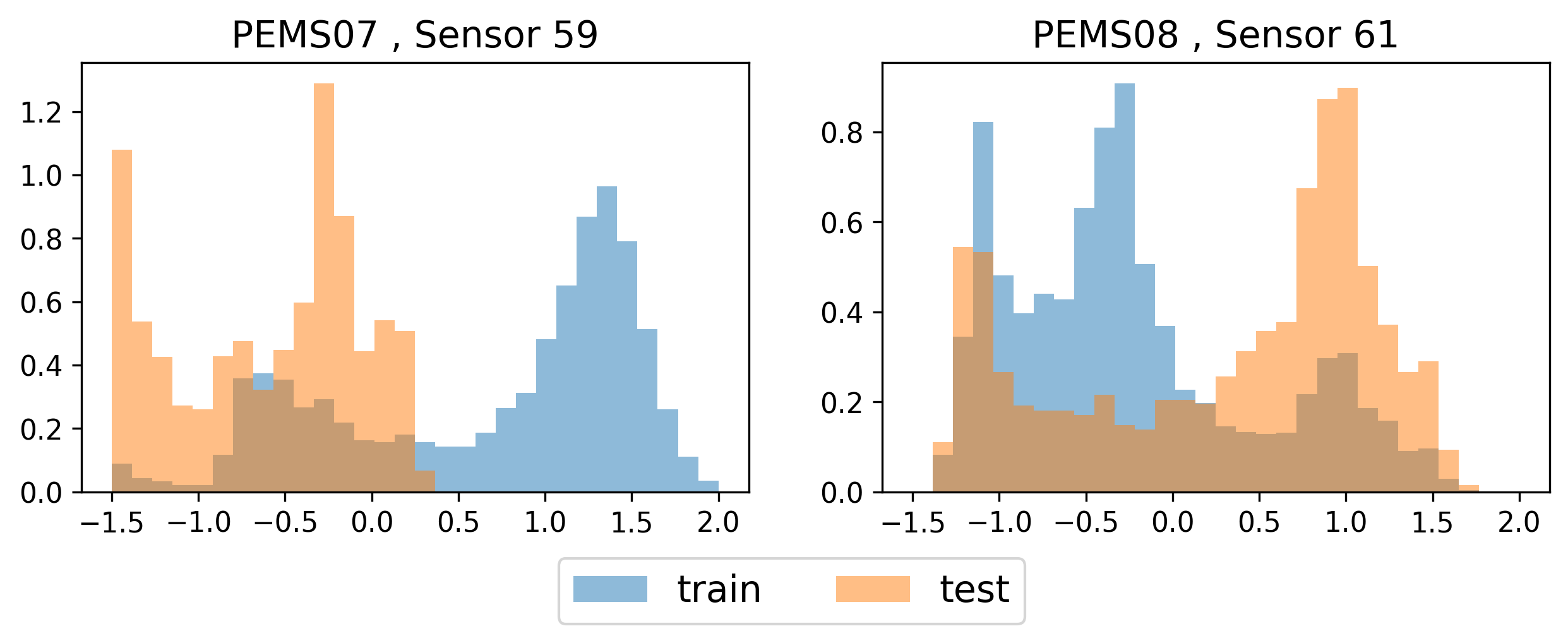
Figure 1: Examples of train & test data distribution shift on PEMS07 and PEMS08 traffic datasets. Data is processed by Z-Score normalization.

Moreover, dealing with the issue of distribution shift between training and testing data has been a common challenge in multivariate time series forecasting (Kim et al. 2021). This shift can have negative impacts, including problems related to overfitting. It’s important to highlight that this distribution shift problem also emerges in various spatio-temporal forecasting tasks, even after datasets have been normalized, as shown in Figure 1. Recent research has introduced a technique called ”channel-independence” (CI) to tackle distribution shift and mitigate overfitting in long-term time series forecasting (Han, Ye, and Zhan 2023; Nie et al. 2023). To elaborate, CI involves using only the historical data within a single channel to predict future time steps within that same channel, without directly incorporating any information from other channels. In the context of spatio-temporal forecasting tasks, CI can be understood as predicting the future data of a specific node without depending on data from other nodes.

However, CI has not found widespread application in spatio-temporal data analysis, particularly when prior predefined graph structures are involved. Many models tend to capture spatio-temporal correlations within data by employing various techniques along both the temporal and spatial dimensions, often leading to channel-mixing (CM). CM stands in contrast to the concept of CI. This prompts us to think: is it feasible to harness the benefits of CI while simultaneously retaining the ability to capture the underlying spatio-temporal relationships within traffic patterns?

In this paper, we propose a spatio-temporal MLP (ST-MLP), a cascaded channel-independent framework for efficient traffic forecasting. The main contributions of our work can be summarized as follows:

• We propose a concise structure that is solely based on MLPs, ensuring its simplicity and efficiency.

• To our best knowledge, our work is the first one to apply the channel-independence strategy in spatio-temporal forecasting problems while incorporating information from predefined graphs.

• In an effort to enhance the integration of diverse embeddings, we implement a cascaded structure. Comparative analysis demonstrates that this method outperforms the conventional approach of simple concatenation.

• Extensive evaluation on various traffic datasets show the superiority of ST-MLP by contrasting its results against those of more than 10 state-of-the-art models.

Preliminary

Problem Definition

Formally, a graph $G$ is defined as an ordered pair $(V,E)$, where $V$ represents the set of vertices (or nodes) and $E$ represents the set of edges. In this paper, we construct the adjacency matrix $A$ of $G$ by scaling the normalized Laplacian matrix (Kipf and Welling 2016). Suppose the historical traffic data is embedded on graph $G$ with $C$ multivariate traffic features and $T$ time intervals. Thus, the historical time series feature can be denoted as $X\in\mathbb{R}^{N\times T\times C}$.

The objective of traffic forecasting is to learn a mapping function $f$ that takes historical traffic data $X$ and graph $G$ as inputs to predict future traffic data for $Q$ time intervals, denoted as $\hat{X}\in\mathbb{R}^{N\times Q\times C}$. For simplicity, in this paper, we set $C$ = 1, resulting in $X\in\mathbb{R}^{N\times T}$ and $\hat{X}\in\mathbb{R}^{N\times Q}$. Subsequently, we refer to the first dimension as the channel dimension and the second dimension as the temporal dimension.

Drawing on insights from  Chen et al., we can enhance the forecasting performance by incorporating additional time-related information. Our focus will be specifically on Time in Day (TD) and Day in Week (DW). TD represents the index of a particular time slot within a day, while DW signifies the weekday label. For any given input data $X$, the corresponding TD and DW can be represented as two integral vectors: $T_{td}\in\mathbb{R}^{T}$ and $T_{dw}\in\mathbb{R}^{T}$, respectively, with these vectors remaining consistent across all nodes. The concepts of TD and DW are directly tied to the recurring daily and weekly patterns of traffic flow due to the evident periodic nature of traffic.

Therefore, the forecast task could be expressed as:

$$\hat{X}=f(G,X,T_{td},T_{dw}).$$ (1)

Channel-independence on Spatio-temporal Data

A multivariate time series can be analogously seen as a multi-channel signal. In the context of spatio-temporal forecasting tasks, we designate the spatial dimension as channels, where each of the $N$ nodes corresponds to a distinct channel. Assuming we have an input data denoted as $X_{input}\in\mathbb{R}^{N\times T}$ for processing, there exist three fundamental types of modules:

$$X_{t}=\texttt{TemporalMix}(X_{input}),$$ (2)

$$X_{c}=\texttt{ChannelMix}(X_{input}),$$ (3)

$$X_{tc}=\texttt{TemporalChannelMix}(X_{input}).$$ (4)

In this context, the TemporalMix module maps the temporal dimension of $X_{input}$ into $X_{t}\in\mathbb{R}^{N\times T^{\prime}}$; the ChannelMix module, conversely, maps the channel (spatial) dimension of $X_{input}$ into $X_{t}\in\mathbb{R}^{N^{\prime}\times T}$; and the TemporalChannelMix module operates both dimensions, yielding an output denoted as $X_{tc}\in\mathbb{R}^{N^{\prime}\times T^{\prime}}$. Here, $T^{\prime}$ signifies the intended temporal dimension, while $N^{\prime}$ represents the intended spatial dimension for the output of these three core modules. It is noteworthy that models adopting the CI strategy incorporate solely modules as described in Equation (2), whereas CM models have the flexibility to encompass any of these module types.

The CI approach serves a dual purpose: it not only addresses the challenge of distribution shift but also leads to a reduction in the variance of prediction outcomes (Han, Ye, and Zhan 2023). To preserve the inherent spatio-temporal correlations while reaping the advantages of CI, this paper adopts a strategy wherein all temporal and spatial information, inclusive of the underlying graph structure, is amalgamated within the temporal dimension. This arrangement facilitates the autonomous prediction of each channel while retaining the benefits of independent forecasting.

Proposed Method

In this section, we would like to explain the general ST-MLP structure and its components in details.

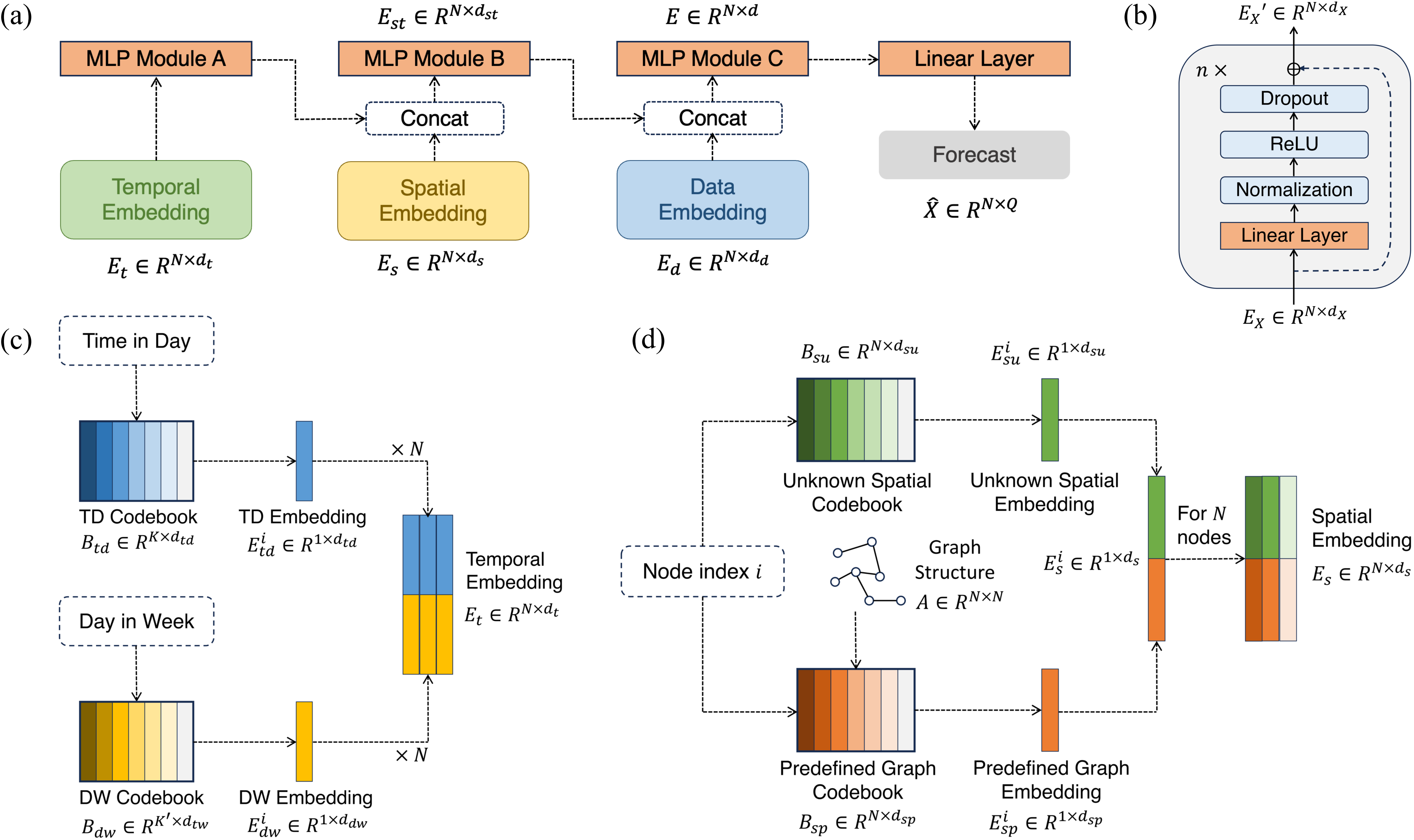
Figure 2: (a) Architecture of ST-MLP. It uses temporal embedding, spatial embedding and data embedding to generate the forecast result. (b) Structure of MLP Module in Figure 2(a). (c) Details of Temporal Embedding, which contains information from Time in Day and Day in Week. (d) Details of Spatial Embedding, which consists of unknown spatial embedding and predefined graph embedding.

General Structure

As illustrated in Figure 2 (a), ST-MLP adopts a cascaded structure to merge different types of information in distinct embeddings. In our study, the symbols marked as $d_{X}$ stand for hyperparameters used to define the temporal dimension of various embeddings. Here, the symbol $X$ acts as a variable that adjusts to different scenarios. Further details about $d_{X}$ and all other symbols are outlined in the Appendix. Specifically, our model takes into account three crucial embeddings: temporal embedding $E_{t}\in\mathbb{R}^{N\times d_{t}}$, which holds crucial temporal details of the traffic data; spatial embedding $E_{s}\in\mathbb{R}^{N\times d_{s}}$, representing the spatial correlations in the traffic graph; and data embedding $E_{d}\in\mathbb{R}^{N\times d_{d}}$. The specifics of each embedding will be explained in the upcoming sections.

In the initial stage, the temporal embedding undergoes processing through the MLP module A. Following this, it gets combined with the spatial embedding in the subsequent stage. This combined data then undergoes processing by the MLP module B, resulting in the creation of a spatio-temporal embedding denoted as $E_{st}\in\mathbb{R}^{N\times d_{st}}$, where $d_{st}=d_{s}+d_{t}$. Moving on to the third stage, the spatio-temporal embedding is merged with the data embedding. Here, the MLP module C is applied, generating a comprehensive embedding $E\in\mathbb{R}^{N\times d}$, where $d=d_{st}+d_{d}$. In the final step, a linear layer is employed to map $E$ to the forecasted outcome $\hat{X}\in\mathbb{R}^{N\times Q}$. It’s important to note that all these operations are carried out within the temporal dimension to ensure the application of the CI strategy.

MLP Module

In Figure 2 (b), the general and straightforward design of the MLP module is depicted. In the cases of modules A, B, and C, we repeat the basic block $n_{A}$, $n_{B}$, and $n_{C}$ times respectively. These values are adjustable hyperparameters. Each basic block encompasses a linear layer that solely operates on the embedding dimension $d_{X}$, a normalization layer for stability during training, a ReLU activation function, a dropout layer to curb overfitting, and a residual connection. It’s worth noting that we maintain the CI strategy within the MLP modules since we are only operating the temporal dimension.

Temporal Embedding

Embedding of Time in Day

Let’s consider a day divided into $K$ time slots equally. When we’re given $T_{td}$, the final time index in $T_{td}$ is used. This index is then transformed into a one-hot vector, $t_{td}\in\mathbb{R}^{1\times K}$, which signifies the Time in Day (TD) index for the entire sequence. Alongside this, there’s a codebook $B_{td}\in\mathbb{R}^{K\times d_{td}}$ that can be learned. In Figure 2 (c), when we perform a dot product of $t_{td}\cdot B_{td}$, we’re essentially selecting the corresponding embedding vector $E_{td}^{i}\in\mathbb{R}^{1\times d_{td}}$ that corresponds to a specific TD index. Since all nodes share the same time information, we can replicate $E_{td}^{i}$ $N$ times to obtain the embedding $E_{td}\in\mathbb{R}^{N\times d_{td}}$, representing the TD details for all nodes.

Embedding of Day in Week

Considering there are $K^{\prime}=7$ days in a week, we can take the index from the end of the sequence $T_{dw}$. This index is transformed into a one-hot vector $t_{dw}\in\mathbb{R}^{1\times K^{\prime}}$ that signifies the Day in Week (DW) index for the entire sequence. Similar to the TD embedding, the embedding of DW $E_{dw}\in\mathbb{R}^{N\times d_{dw}}$ can be obtained from a learnable codebook $B_{dw}\in\mathbb{R}^{K^{\prime}\times d_{dw}}$. This helps us capture weekly patterns.

Temporal Embedding Representation

As shown in Figure 2 (c), $E_{td}$ and $E_{dw}$ are generated paralleled, then are concatenated together:

$$E_{t}=\texttt{Concat}[(E_{td},E_{dw}),\texttt{dim}=1].$$ (5)

Hence, we can derive the general temporal embedding $E_{t}\in\mathbb{R}^{N\times d_{t}}$, where $d_{t}=d_{td}+d_{dw}$.

Spatial Embedding

Embedding of known predefined graph structure

With $A\in\mathbb{R}^{N\times N}$ representing a predefined adjacency matrix, we aim to integrate fixed graph details into the neural network. To achieve this, we start by initializing a learnable codebook $B_{sp}\in\mathbb{R}^{N\times d_{sp}}$. We then utilize matrix multiplication to proceed:

$$AB_{sp}=E_{sp},$$ (6)

where $E_{sp}\in\mathbb{R}^{N\times d_{sp}}$. Next, we employ the node index $i$ to select the appropriate embedding vector $E_{sp}^{i}\in\mathbb{R}^{1\times d_{sp}}$, as illustrated in Figure 2 (d). This approach allows us to include predetermined graph information while retaining the CI principle within the model structure.

Embedding of unknown spatial information

Previous studies underscore that a pre-defined graph may not fully encapsulate all the authentic spatial intricacies inherent in real-world scenarios (Zhang et al. 2020; Guo et al. 2021). To uncover hidden spatial details from traffic data, we introduce an additional learnable codebook $B_{su}\in\mathbb{R}^{N\times d_{su}}$ to signify inherent spatial characteristics. Similar to the procedure discussed in the preceding paragraph while learning $E_{sp}^{i}$, we acquire $E_{su}^{i}\in\mathbb{R}^{1\times d_{su}}$ for node $i$.

Spatial Embedding Representation

In Figure 2 (d), similar to the approach used for temporal representation, the overall spatial representation is obtained by concatenating two spatial embeddings:

$$E_{s}^{i}=\texttt{Concat}[(E_{sp}^{i},E_{su}^{i}),\texttt{dim}=1].$$ (7)

By repeating this for all $N$ nodes, we can get the final spatial embedding $E_{s}\in\mathbb{R}^{N\times d_{s}}$, where $d_{s}=d_{sp}+d_{su}$.

Data Embedding

We replicate $T_{td}$ for $N$ times, resulting in $T_{td}^{\prime}\in\mathbb{R}^{N\times T}$. Similarly, we repeat the procedure with $T_{dw}$ to generate $T_{dw}^{\prime}\in\mathbb{R}^{N\times T}$. As for the data embedding, we concatenate $X$, $T_{td}^{\prime}$, and $T_{dw}^{\prime}$ to construct a representation that encapsulates both the original traffic data and time stamps. Ultimately, a linear transformation is employed to map the temporal dimension to $d_{d}$:

$$E_{d}=\texttt{Linear}(\texttt{Concat}[(X,T_{td}^{\prime},T_{dw}^{\prime}),\texttt{dim}=1]),$$ (8)

where $E_{d}\in\mathbb{R}^{N\times d_{d}}$.

Experiments

Datasets

We employ four widely used public traffic datasets to conduct a comparative analysis of forecasting performance. These datasets encompass a variety of traffic data types, including traffic speed and volume. Specifically, we utilize the PEMS-BAY dataset for traffic speed and the PEMS04, PEMS07, and PEMS08 datasets for traffic volume, as documented by Chen et al. (Chen et al. 2001; Liang et al. 2023). The traffic measurements in these datasets are collected from loop sensors situated on highway networks. These measurements are aggregated into 5-minute intervals and subsequently subjected to Z-Score normalization. Our data is divided into three subsets: training (70%), validation (10%), and testing (20%).

Baseline Methods

We compare the proposed model (ST-MLP) with the following methods for traffic forecasting. For conventional method, we choose Historical Inertia (HI) (Cui, Xie, and Zheng 2021). For STGNNs Methods, we choose Graph WaveNet (Wu et al. 2019), DCRNN (Li et al. 2017), AGCRN (Bai et al. 2020), STGCN (Yu, Yin, and Zhu 2017), StemGNN (Cao et al. 2020), GTS (Shang, Chen, and Bi 2021), MTGNN (Wu et al. 2020), DGCRN (Li et al. 2023). For time series forecasting methods. we choose DLinear (Zeng et al. 2023), and PatchTST (Nie et al. 2023). In addition, we also apply two innovative methods: STID (Shao et al. 2022a) and STNorm (Deng et al. 2021).

We use BasicTS and Easytorch  (Wang 2020; Liang et al. 2023) to implement baseline models. To ensure fair and consistent evaluations, all baseline models are assessed under identical environments. Details are provided in  Appendix.

Implementation Details

In our traffic forecasting benchmarks, we adopt a historical data approach involving a 12-step strategy. This approach uses the last 12 observations, equivalent to a 1-hour interval, to predict the upcoming 12-step observations, also spanning an hour. We consider time intervals of 3 steps (15 minutes), 6 steps (30 minutes), and 12 steps (60 minutes) between historical inputs and target forecasts. Additionally, we evaluate the average performance over the 12 steps. Given that the datasets’ time intervals are 5 minutes each, a single day is divided into 288 time intervals. Consequently, the parameter $K$ for embedding Time in Day is set to 288. The training process for all models takes place on an AMD EPYC 7642 Processor @ 2.30GHz with a single RTX 3090 (24GB) GPU.

In natural language processing tasks, Layer Normalization is often favored over Batch Normalization. However, in time series tasks, this issue is still a subject of debate (Nie et al. 2023). We consider this as a critical hyperparameter in our experiments. To assess the performance of all methods, we employ three metrics: Mean Absolute Error (MAE), Root Mean Square Error (RMSE), and Mean Absolute Percentage Error (MAPE). All the necessary settings for reproducing our results are available in our code and Appendix.

Datasets Methods 15 min 30 min 60 min Average MAE RMSE MAPE MAE RMSE MAPE MAE RMSE MAPE MAE RMSE MAPE PEMS-BAY HI 3.06 7.05 6.85% 3.06 7.04 6.84% 3.05 7.03 6.83% 3.05 7.05 6.84% GraphWaveNet 1.31 2.76 2.75% 1.66 3.77 3.76% 1.98 4.58 4.69% 1.60 3.69 3.60% DCRNN 1.31 2.76 2.73% 1.65 3.75 3.70% 1.97 4.58 4.66% 1.59 3.68 3.57% AGCRN 1.35 2.83 2.91% 1.66 3.76 3.80% 1.93 4.46 4.57% 1.60 3.65 3.64% STGCN 1.36 2.82 2.87% 1.70 3.82 3.86% 2.01 4.59 4.73% 1.64 3.73 3.70% StemGNN 1.57 3.26 3.45% 2.12 4.67 4.95% 2.80 6.16 6.78% 2.09 4.72 4.89% GTS 1.36 2.87 2.85% 1.72 3.84 3.88% 2.05 4.60 4.87% 1.66 3.75 3.73% MTGNN 1.33 2.80 2.78% 1.64 3.73 3.71% 1.93 4.48 4.60% 1.58 3.63 3.56% DGCRN 1.33 2.76 2.74% 1.65 3.74 3.67% 1.98 4.58 4.62% 1.62 3.68 3.58% DLinear 1.58 3.41 3.28% 2.15 4.89 4.71% 2.97 6.76 6.89% 2.14 5.04 4.72% PatchTST 1.55 3.38 3.26% 2.12 4.92 4.67% 2.98 6.93 6.88% 2.12 5.10 4.71% STID 1.31 2.78 2.74% 1.63 3.70 3.68% 1.90 4.39 4.48% 1.56 3.60 3.51% STNorm 1.33 2.82 2.78% 1.65 3.78 3.68% 1.91 4.45 4.47% 1.58 3.66 3.51% ST-MLP 1.32 2.78 2.77% 1.62 3.65 3.67% 1.90 4.34 4.45% 1.56 3.55 3.50% PEMS04 HI 42.33 61.64 29.90% 42.35 61.66 29.92% 42.38 61.67 29.96% 42.35 61.66 29.92% GraphWaveNet 17.68 28.53 12.46% 18.58 29.97 13.20% 20.01 31.98 14.22% 18.57 29.92 13.09% DCRNN 18.49 29.55 12.62% 19.58 31.27 13.32% 21.40 33.84 14.75% 19.59 31.28 13.37% AGCRN 18.41 29.50 12.49% 19.31 30.99 13.50% 20.48 32.75 14.19% 19.24 30.88 13.30% STGCN 18.74 29.94 13.02% 19.65 31.47 13.61% 21.27 33.79 14.73% 19.69 31.47 13.67% StemGNN 19.70 31.30 13.56% 21.83 34.50 15.15% 26.22 40.76 18.20% 22.17 35.12 15.41% GTS 19.29 30.49 13.30% 20.88 32.83 14.62% 23.56 36.38 16.92% 20.94 32.92 14.71% MTGNN 18.12 29.50 12.44% 18.97 31.09 12.91% 20.42 33.27 13.79% 18.97 31.04 12.93% DGCRN 18.85 29.95 12.92% 20.04 32.07 13.50% 22.32 36.28 14.61% 20.29 32.55 13.60% DLinear 22.28 34.95 14.84% 26.97 41.79 18.42% 37.37 56.55 25.47% 27.94 43.89 19.07% PatchTST 22.28 34.74 14.62% 27.06 41.73 17.79% 37.73 56.80 25.21% 28.08 43.89 18.58% STID 17.52 28.57 11.96% 18.34 29.98 12.48% 19.66 31.98 13.40% 18.34 29.95 12.47% STNorm 18.47 31.17 12.90% 19.27 32.99 13.05% 20.47 34.43 13.71% 19.21 32.56 13.10% ST-MLP 17.32 28.41 11.92% 18.08 29.83 12.32% 19.18 31.52 12.89% 18.05 29.72 12.28% PEMS07 HI 49.02 71.15 22.73% 49.04 71.18 22.75% 49.06 71.21 22.79% 49.03 71.18 22.75% GraphWaveNet 18.72 30.62 7.86% 20.19 33.17 8.53% 22.46 36.59 9.65% 20.14 33.06 8.54% DCRNN 19.44 31.22 8.22% 21.12 34.13 8.93% 24.04 38.44 10.34% 21.14 34.13 8.99% AGCRN 19.35 31.87 8.17% 20.74 34.74 8.78% 22.84 38.32 9.79% 20.71 34.65 8.86% STGCN 20.59 33.30 8.78% 21.98 36.09 9.28% 24.51 40.26 10.72% 22.03 36.14 9.42% StemGNN 19.79 32.12 8.52% 21.91 35.63 9.42% 25.65 41.05 11.15% 22.03 35.81 9.54% GTS 20.11 31.92 8.53% 22.27 35.11 9.46% 25.72 39.96 11.08% 22.24 35.17 9.47% MTGNN 19.33 31.20 8.56% 20.93 34.16 8.90% 23.52 38.21 10.14% 20.93 34.14 9.08% DGCRN 19.03 30.74 8.16% 20.41 33.27 8.69% 22.58 36.74 9.63% 20.44 33.25 8.73% DLinear 24.71 38.05 9.84% 30.56 46.90 13.87% 43.70 65.37 20.42% 31.72 49.43 14.52% PatchTST 24.73 37.97 10.32% 30.75 47.06 12.92% 44.21 66.02 18.97% 31.98 49.68 13.54% STID 18.37 30.40 7.77% 19.64 32.86 8.29% 21.53 36.11 9.26% 19.59 32.77 8.30% STNorm 19.15 31.68 8.04% 20.58 34.88 8.63% 22.66 38.51 9.75% 20.50 34.66 8.69% ST-MLP 18.30 30.33 7.68% 19.55 32.69 8.27% 21.43 35.86 9.19% 19.51 32.61 8.26% PEMS08 HI 36.65 50.44 21.60% 36.66 50.45 21.63% 36.68 50.46 21.68% 36.66 50.45 21.63% GraphWaveNet 13.57 21.66 9.00% 14.48 23.46 9.33% 15.90 25.89 10.31% 14.47 23.46 9.34% DCRNN 14.07 22.14 9.23% 15.14 24.18 9.91% 16.84 26.87 11.12% 15.13 24.13 9.93% AGCRN 14.28 22.51 9.37% 15.32 24.41 9.93% 17.01 27.03 11.07% 15.35 24.45 10.01% STGCN 14.93 23.41 9.78% 15.92 25.25 10.19% 17.70 27.86 11.56% 15.98 25.26 10.43% StemGNN 14.98 23.56 10.64% 16.49 26.29 11.38% 19.26 30.37 13.20% 16.62 26.42 11.65% GTS 15.03 23.54 9.49% 16.48 26.00 10.50% 19.00 29.57 12.44% 16.54 26.02 10.60% MTGNN 14.23 22.32 9.98% 15.24 24.33 10.22% 16.86 26.85 12.13% 15.27 24.29 10.59% DGCRN 13.79 21.91 9.13% 14.81 23.83 9.74% 16.39 26.34 11.02% 14.85 23.84 9.84% DLinear 17.75 24.49 11.16% 21.62 34.85 13.33% 30.42 46.33 20.12% 22.42 35.44 14.28% PatchTST 17.81 27.58 10.76% 21.77 34.03 13.10% 30.76 46.86 18.43% 22.60 35.68 13.62% STID 13.32 21.61 8.79% 14.21 23.52 9.33% 15.61 25.91 10.39% 14.23 23.48 9.40% STNorm 14.42 22.85 9.17% 15.41 24.97 9.85% 16.88 27.68 10.70% 15.37 24.91 9.82% ST-MLP 13.12 21.29 8.59% 14.03 23.10 9.30% 15.41 25.48 10.17% 14.03 23.07 9.25%

Table 1: Results on various traffic datasets. MAE, MSE and MAPE for 3, 6, 12 horizons as well averaged over a one-hour (12 steps) are reported. Best results are bold marked. ST-MLP achieves the best performance overall.

Experimental Result

The outcomes of the model comparison are detailed in Table 1. All baseline models exhibit significant improvements over the HI model, indicating their proficiency in capturing the underlying spatio-temporal patterns in the provided data. As the prediction horizon lengthens, the precision of all models declines, underscoring the challenge of time series forecasting as the prediction timeframe extends further into the future.

In the case of the traffic speed dataset PEMS-BAY, our model attains the highest overall accuracy compared to other advanced STGNNs. Moreover, some basic baseline models, like STID, also demonstrate competitive results. This suggests that crafting effective traffic forecasting algorithms might not always need intricate neural network architectures.

Concerning the traffic flow datasets PEMS04, PEMS07, and PEMS08, our model exhibits superior performance and consistently surpasses the baseline methods by a considerable margin. It’s worth noting that approaches specifically tailored for multivariate time series forecasting (DLinear, PatchTST), without incorporating spatial characteristics, understandably exhibit diminished performance in the context of spatio-temporal forecasting.

Efficiency Study compared to STGNNs methods

Since ST-MLP outperforms all the STGNNs method, in this section, we conduct a comparison of the efficiency of ST-MLP with other STGNNs methods using all datasets. To ensure a more intuitive and effective comparison, we analyze the average training time required for one epoch of these models. To get a better visualization in various datasets, in each dataset we normalize the highest time consumption to 1, then the time of other models are also normalized correspondingly.

The normalized training time consumption is illustrated in Figure 3. In contrast to other STGNN methods, our ST-MLP achieves exceptional computational speed benefiting from its simplicity. This underscores the efficiency of our proposed approach. Among the STGNN methods, StemGNN and MTGNN demonstrate relatively favorable computational efficiency, although their accuracy is not exceptional.

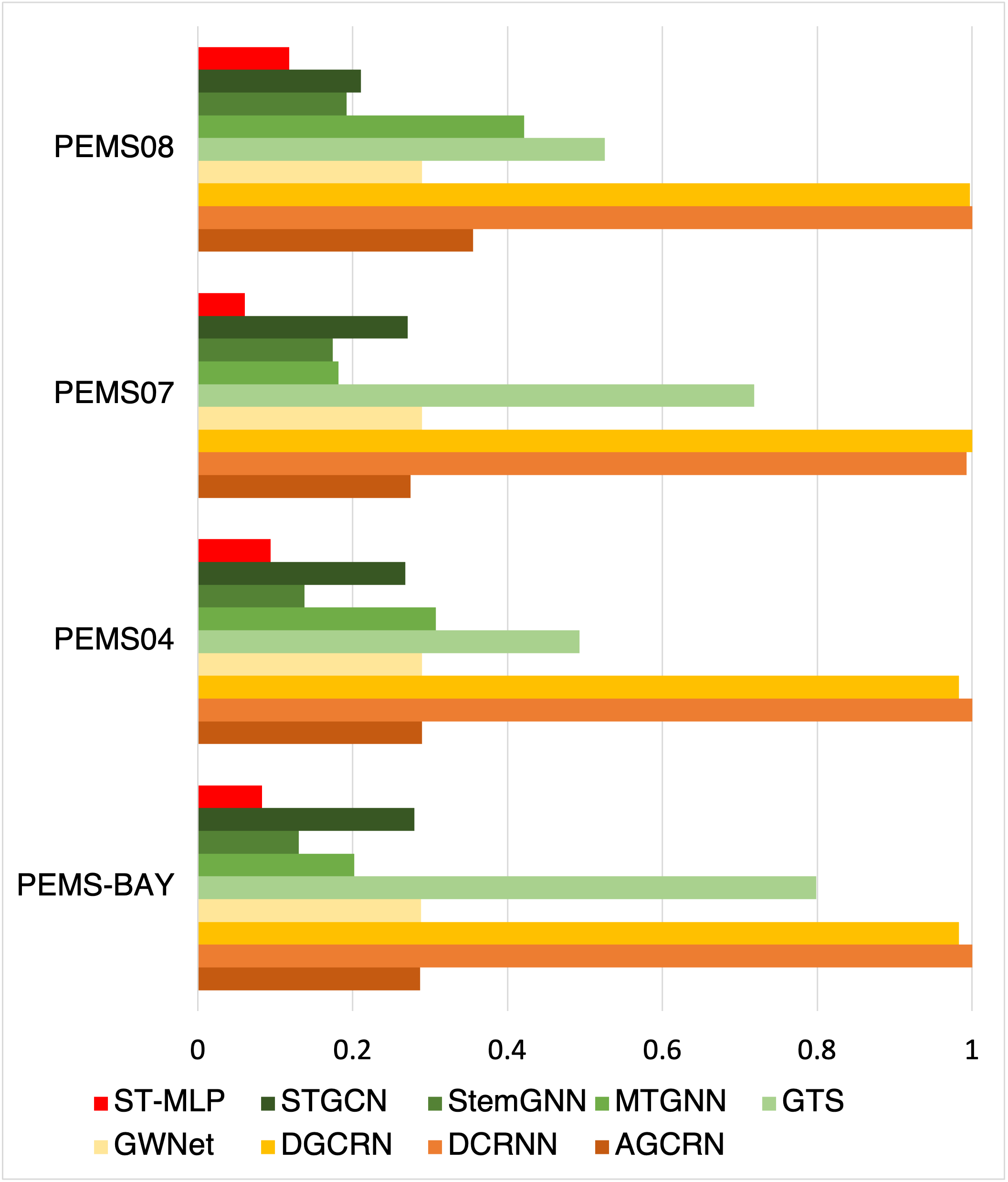
Figure 3: Normalized training time for one epoch. The slowest model is normalized to 1 on each experiment dataset. ST-MLP requires significantly less training time than other STGNNs counterparts on all datasets.

Ablation Study

Due to space constraints, the ablation study primarily presents experiment results conducted on specific datasets. Nevertheless, it’s important to acknowledge that similar conclusions and analyses are applicable to PEMS-BAY, PEMS04, PEMS07, and PEMS08 datasets as well.

Importance of Different Embedding Components

In this section, we conduct ablation studies to assess the effectiveness of the four different embeddings in our ST-MLP model. Specifically, we examine four variants of the ST-MLP: one without Time in Day information ($E_{td}$), one without Day in Week information ($E_{dw}$), one without predefined graph information ($E_{sp}$), and one without the unknown spatial embedding ($E_{su}$). For each variant, we analyze its performance in comparison to the complete ST-MLP model. By systematically removing specific embeddings, our goal is to discern their individual contributions to the overall forecasting accuracy. The test MAE values of these ST-MLP variants are illustrated in Figure 4.

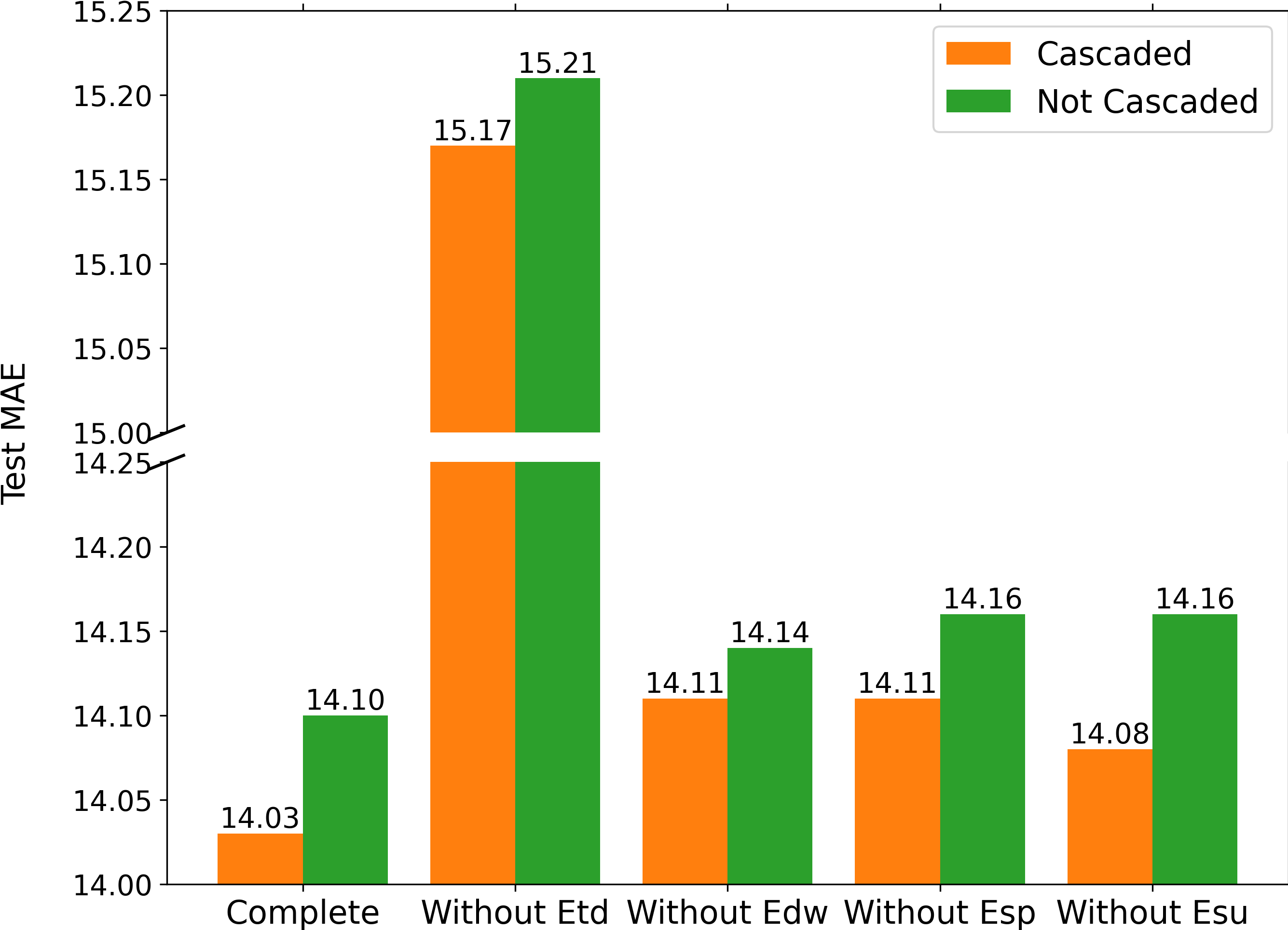
Figure 4: Test MAE of variants of ST-MLP on PEMS08. The cascaded model with complete embeddings achieves the lowest test error among all variants.

In summary, the ablation studies demonstrate that all embeddings play a positive role in improving the final forecasting accuracy. Among the four embeddings analyzed, Time in Day ($E_{td}$) emerges as the most crucial feature, indicating that capturing the daily seasonal traffic trends is essential for achieving accurate forecasts.

In this framework, the combination of predefined graph connections and the exploration of more spatial features contributes to improved accuracy. Leveraging spatial information through graph connections and additional features enhances the model’s capability to capture traffic patterns, thereby further enhancing the accuracy of traffic forecasting.

Importance of Cascaded Structure

To demonstrate the efficacy of the cascaded structure, we propose other variants of ST-MLP which are not cascaded, denoted by the green bars in Figure 4. Rather than adopting sequential aggregation of $E_{t}$, $E_{s}$, and $E_{d}$ as depicted in Figure 2 (a), we opt for a parallel concatenation strategy: $E=\texttt{Concat}[(E_{t},E_{s},E_{d}),\texttt{dim}=1]$. Subsequently, we employ a linear layer to transform this into the forecast result $\hat{X}\in R^{N\times Q}$.

Our results underscore the important role of the cascaded structure in bolstering the model’s performance. Remarkably, the complete cascaded model demonstrates the best performance, while a consistent improvement is observed in the cascaded model compared to its non-cascaded counterparts, even when specific embeddings are absent. This lends empirical support to the effectiveness of our cascaded design across a broad range of cases.

Ablation on Channel-independence

Typically, spatial information is commonly utilized by mixing channels, such as Graph Neural Networks (GNNs) or Graph Convolutional Networks (GCNs), which is opposite to CI. To investigate the impact of CI vs CM strategy, we introduce a variant of ST-MLP. We add a simple linear layer before the forecast in Figure 2 (a) to mix the channels, which belongs to the ChannelMix module type in Equation (3), creating a new variant named ”CM ST-MLP”. We then recorded the metrics on the training, validation, and testing datasets of PEMS-BAY, PEMS04, and PEMS08. The results are presented in Table 2.

The outcomes demonstrate a potential issue with the CM ST-MLP model. Despite having similar validation errors compared to the original CI ST-MLP model, CM ST-MLP exhibits lower training error but much higher testing error. This more severe overfitting problem indicates that even a simple linear operation to mix channels can negatively impact the model’s generalization ability when compared to the CI training strategy used in ST-MLP.

The overfitting issue observed in the CM ST-MLP model can be attributed to a couple of potential reasons, primarily the distribution shift problem, where the difference between the train and test distributions could degrade model performance As we observed in Figure 1, in real-world applications, the existence of non-stationary time series is quite common, which makes robustness against distribution shift crucial. Recent studies reveal that the choice between CM and CI is a trade-off between robustness and capacity (Han, Ye, and Zhan 2023). While CM models are more expressive, they might inadvertently capture false spatio-temporal correlations due to the mixing on spatial channel. On the other hand, the CI training strategy in our ST-MLP could alleviate the problem of data distribution shift, leading to improved generalization and more accurate traffic forecasting.

Conclusion and Future Work

In this study, we have introduced a novel model for accurate traffic forecasting, termed ST-MLP. By leveraging the CI strategy and simple MLPs, our framework achieves competitive forecasting accuracy. The evaluation metrics we employ underscore the effectiveness of our approach. We anticipate that this work will inspire the exploration of straightforward models in the domains of traffic and spatio-temporal forecasting, offering valuable insights for both neural architecture understanding and practical applications.

To expand upon our research, it would be worthwhile to extend our analysis to diverse spatio-temporal datasets and delve into enhancing robustness using CI strategies. Additionally, considering the faster convergence rate and mitigation of over-smoothing associated with CI (Nie et al. 2023; Zhou et al. 2022b) present interesting avenues for future exploration.

Dataset Stage CI ST-MLP CM ST-MLP MAE RMSE MAPE MAE RMSE MAPE PEMS-BAY Training 1.41 3.11 3.05% 1.40 3.04 3.06% Validation 1.56 3.31 3.58% 1.68 3.39 3.86% Testing 1.56 3.55 3.50% 1.75 3.73 3.92% PEMS04 Training 16.75 27.61 12.60% 16.52 27.15 12.95% Validation 17.76 28.40 12.18% 19.41 30.44 13.90% Testing 18.05 29.72 12.28% 20.74 33.85 14.60% PEMS08 Training 14.11 23.54 9.64% 13.25 21.34 8.99% Validation 14.11 23.19 10.67% 14.12 22.45 9.78% Testing 14.03 23.08 9.22% 15.58 25.21 10.34%

Table 2: CI vs CM strategies on ST-MLP. The CM ST-MLP model displays lower training error but higher testing error compared to the CI variant

Related Works

Traffic Forecasting

As a key component of ITS, traffic forecasting has been the subject of study for decades. As early as 1979, AutoRegressive Integrated Moving Average (ARIMA) models are utilized to forecast freeway traffic data (Williams and Hoel 2003). Over time, numerous machine learning-based methods have been explored for this task, including Support Vector Machine (SVM) (Zhang and Liu 2009), Decision Tree (Xia and Chen 2017), Bayesian Networks (Sun, Zhang, and Yu 2006), among others.

Deep learning has revolutionized traffic forecasting algorithms, offering greater flexibility and complexity by designing neural structures for specific functions in different layers. Long Short-Term Memory (LSTM) neural networks have been effectively applied to tackle traffic forecasting tasks, leveraging their ability to handle sequential data (Zhao et al. 2017). Another approach by Zhang et al. involved representing the traffic network as a regular 2D grid and using traditional Convolutional Neural Networks (CNNs) to forecast traffic data (Zhang et al. 2019).

Graph neural networks (GNNs) are well-suited for traffic research, as road networks can be effectively represented by graph structures (Chen, Segovia-Dominguez, and Gel 2021). For instance, some papers utilize the attention mechanism to analyze spatial and temporal correlations in traffic data (Guo et al. 2019; Zheng et al. 2020). Xu et al. leverage the combination of graph structure and transformer framework to achieve high forecast accuracy (Xu et al. 2020). Moreover, several models have explored dynamic graph structures to better capture temporal-spatial relationships, moving beyond fixed and predefined road graphs (Zhang et al. 2020; Guo et al. 2021). These approaches demonstrate the effectiveness of GNNs in incorporating spatio-temporal information for improved traffic forecasting performance.

Linear Models for Time Series Forecasting

Recent years have seen a surge in research in the field of time series forecast, particularly the transformer-based models, including Informer (Zhou et al. 2021), Autoformer (Wu et al. 2021), Fedformer (Zhou et al. 2022a), Pyraformer (Liu et al. 2021), etc. However, Zeng et al. demonstrated that using some simple linear models can outperform many transformer architectures in long-term time series forecasting tasks (Zeng et al. 2023). Since MLP structures have less complexity and computational cost, they have also garnered attention from researchers. For instance, Ekambaram et al. followed the idea of MLP mixer in computer vision (Tolstikhin et al. 2021) and performed mixing operations along both the time and feature dimensions in their TSMixer model (Ekambaram et al. 2023). There are also some more emerging MLP-based designs like Koopa (Liu et al. 2023b) and FITS (Xu, Zeng, and Xu 2023), further highlighting the potential of MLP-based approaches in time series forecasting.

Appendix A Appendix

Notation

In this section, we provide a comprehensive definition about all notation in the section Proposed Method, summarized in Table 3.

Notation	Description
$A$	Predefined graph matrix
$B_{td}$	Codebook of Time in Day (TD)
$B_{dw}$	Codebook of Day in Week (DW)
$B_{sp}$	Codebook of predefined graph structure
$B_{su}$	Codebook of unknown spatial information
$E_{t}$	Temporal embedding
$E_{td}$	Temporal embedding of TD
$E_{td}^{i}$	$E_{td}$ for node $i$
$E_{dw}$	Temporal embedding of DW
$E_{dw}^{i}$	$E_{dw}$ for node $i$
$E_{s}$	Spatial embedding
$E_{s}^{i}$	$E_{s}$ for node $i$
$E_{su}$	Unknown spatial embedding
$E_{su}^{i}$	$E_{su}$ for node $i$
$E_{sp}$	Predefined graph embedding
$E_{sp}^{i}$	$E_{sp}$ for node $i$
$E_{st}$	Spatio-temporal embedding generated as the output of MLP module B
$E_{d}$	Data Embedding
$E$	The entire embedding generated as the output of MLP module C
$E_{X}$	Example of MLP module input denoted by ”X”
$E_{X}^{\prime}$	Example of MLP module output denoted by ”X”
$d_{X}$	Temporal dimension of $E_{X}$ and $E_{X^{\prime}}$
$d_{t}$	Temporal dimension of $E_{t}$
$d_{td}$	Temporal dimension of $B_{td}$
$d_{dw}$	Temporal dimension of $B_{dw}$
$d_{s}$	Temporal dimension of $E_{s}$
$d_{su}$	Temporal dimension of $B_{su}$
$d_{sp}$	Temporal dimension of $B_{sp}$
$d_{st}$	Temporal dimension of $E_{st}$
$d_{d}$	Temporal dimension of $E_{d}$
$d$	Temporal dimension of $E$
$K$	Count of discrete time intervals in a day
$K^{\prime}$	Count of days in a week
$N$	Number of nodes/sensors
$N^{\prime}$	Intended spatial dimension of CM model
$n_{A}$	Number of blocks in MLP module A
$n_{B}$	Number of blocks in MLP module B
$n_{C}$	Number of blocks in MLP module C
$Q$	Target / Forecast window
$T$	Context / Look-back window
$T^{\prime}$	Intended temporal dimension of CM/CI model
$T_{td}$	Input sequence with TD information
$T_{dw}$	Input sequence with DW information
$t_{td}$	One-hot vector transformed from the last value of $T_{td}$
$t_{dw}$	One-hot vector transformed from the last value of $T_{dw}$
$X$	Input data
$\hat{X}$	Output / Forecast result

Table 3: Notations in ST-MLP.

Dataset Description

Our experiments encompass a traffic speed dataset and three traffic volume datasets, as summarized in Table 4.

Traffic Speed Dataset

PEMS-BAY comprises six months of speed data collected from 325 static detectors situated in the San Francisco South Bay Area.

Traffic Volumne Dataset

PEMS04, PEMS07, and PEMS08 are traffic volume flow datasets that provide real-time highway traffic volume information in California. These datasets are sourced from the Caltrans Performance Measurement System (PeMS) and are collected at 30-second intervals. The raw traffic flow data is subsequently aggregated into 5-minute intervals.

Dataset	PEMS-BAY	PEMS04	PEMS07	PEMS08
Type	Speed	Volumes	Volumes	Volumes
Time Span	5 months	2 months	3 months	2 months
Num of Nodes	325	307	883	170
Record Steps	5 mins	5 mins	5 mins	5 mins

Table 4: Statistics of datasets.

Baseline Methods

We compare the proposed model (ST-MLP) with the following methods for traffic forecasting:

• Historical Inertia (HI) (Cui, Xie, and Zheng 2021): A baseline method that utilizes the most recent historical data points in the input time series.

• Graph WaveNet (Wu et al. 2019): A framework that combines an adaptive adjacency matrix with graph convolution and 1D dilated convolution.

• DCRNN (Li et al. 2017): A module that integrates graph convolution into an encoder-decoder gated recurrent unit.

• AGCRN (Bai et al. 2020): Graph convolution recurrent networks incorporating adaptive graphs to capture dynamic spatial features.

• STGCN (Yu, Yin, and Zhu 2017): A framework that combines graph convolution and a 1D convolution unit together.

• StemGNN (Cao et al. 2020): A structure that captures inter-series correlations and temporal dependencies jointly in the spectral domain.

• GTS (Shang, Chen, and Bi 2021): A graph neural network structure that extracts unknown graph information.

• MTGNN (Wu et al. 2020): A module that developed based on a WaveNet backbone.

• DGCRN (Li et al. 2023): A graph convolution recurrent network which generates a dynamic graph at each time step.

• DLinear (Zeng et al. 2023): A simple MLP framework with the CI strategy designed for long-term time series forecasting.

• PatchTST (Nie et al. 2023): A Transformer-based model with the CI strategy designed for long-term time series forecasting.

• STID (Shao et al. 2022a): Spatial-temporal identity, an effective MLP method by attaching spatial and temporal identity information.

• STNorm (Deng et al. 2021): An innovative technique that applies spatial normalization and temporal normalization.

Implementation Platform

We train all the models on the AMD EPYC 7642 Processor @ 2.30GHz with a single RTX 3090 (24GB) GPU. We modify the codes from BasicTS  (Liang et al. 2023) and easytorch  (Wang 2020) to implement our model and all baselines.

Hyperparameters

The hyperparameters used for reproducing our experiment results are shown in the Table 5.

Dataset PEMS-BAY PEMS04 PEMS07 PEMS08 batchsize 32 learning_rate 0.002 weight_decay 0.0001 gamma 0.5 milestones [1, 50, 80] num_epochs 200 $n_{A}$ 1 $n_{B}$ 1 $n_{C}$ 3 $d_{d}$ 96 $d_{su}$ 32 $d_{sp}$ 32 $d_{td}$ 32 $d_{dw}$ 32 32 16 32 Normalization LayerNorm BatchNorm

Table 5: Hyperparameters for ST-MLP implementation.

Efficiency Study

In this section, we aim to present the raw training times for each epoch of various STGNN models and ST-MLP across different datasets. Table 6 clearly illustrates that ST-MLP boasts the shortest training time among them.

Dataset	PEMS-BAY	PEMS04	PEMS07	PEMS08
Methods	Seconds/epoch
AGCRN	62.82	16.48	86.55	12.71
DCRNN	219.12	56.93	312.73	35.78
DGCRN	215.29	55.95	314.96	35.68
GWNet	63.13	16.46	91.23	10.35
GTS	174.94	28.07	226.28	18.81
MTGNN	44.29	17.50	57.25	15.07
StemGNN	28.51	7.85	54.76	6.87
STGCN	61.21	15.26	85.32	7.53
ST-MLP	18.22	5.34	19.05	4.23

Table 6: Absolute training time for one epoch in different datasets. ST-MLP achieves the best efficiency.

References

- Bai et al. (2020) Bai, L.; Yao, L.; Li, C.; Wang, X.; and Wang, C. 2020. Adaptive Graph Convolutional Recurrent Network for Traffic Forecasting. Advances in Neural Information Processing Systems, 33: 17804–17815.
- Cao et al. (2020) Cao, D.; Wang, Y.; Duan, J.; Zhang, C.; Zhu, X.; Huang, C.; Tong, Y.; Xu, B.; Bai, J.; Tong, J.; et al. 2020. Spectral Temporal Graph Neural Network for Multivariate Time-series Forecasting. Advances in Neural Information Processing Systems, 33: 17766–17778.
- Chen et al. (2001) Chen, C.; Petty, K. F.; Skabardonis, A.; Varaiya, P. P.; and Jia, Z. 2001. Freeway Performance Measurement System: Mining Loop Detector Data. Transportation Research Record, 1748: 102 – 96.
- Chen, Segovia-Dominguez, and Gel (2021) Chen, Y.; Segovia-Dominguez, I.; and Gel, Y. R. 2021. Z-gcnets: Time Zigzags at Graph Convolutional Networks for Time Series Forecasting. In Proceedings of the International Conference on Machine Learning.
- Cui, Xie, and Zheng (2021) Cui, Y.; Xie, J.; and Zheng, K. 2021. Historical Inertia: A Neglected But Powerful Baseline for Long Sequence Time-series Forecasting. In Proceedings of the 30th ACM International Conference on Information & Knowledge Management, 2965–2969.
- Das et al. (2023) Das, A.; Kong, W.; Leach, A.; Sen, R.; and Yu, R. 2023. Long-term Forecasting with TiDE: Time-series Dense Encoder. arXiv:2304.08424.
- Deng et al. (2021) Deng, J.; Chen, X.; Jiang, R.; Song, X.; and Tsang, I. W. 2021. St-norm: Spatial and temporal normalization for multi-variate time series forecasting. In Proceedings of the 27th ACM SIGKDD Conference on Knowledge Discovery & Data Mining, 269–278.
- Ekambaram et al. (2023) Ekambaram, V.; Jati, A.; Nguyen, N.; Sinthong, P.; and Kalagnanam, J. 2023. TSMixer: Lightweight MLP-mixer Model for Multivariate Time Series Forecasting. arXiv:2306.09364.
- Guo et al. (2019) Guo, S.; Lin, Y.; Feng, N.; Song, C.; and Wan, H. 2019. Attention Based Spatial-temporal Graph Convolutional Networks for Traffic Flow Forecasting. In Proceedings of the AAAI Conference on Artificial Intelligence, 01, 922–929.
- Guo et al. (2021) Guo, S.; Lin, Y.; Wan, H.; Li, X.; and Cong, G. 2021. Learning Dynamics And Heterogeneity of Spatial-temporal Graph Data for Traffic Forecasting. IEEE Transactions on Knowledge and Data Engineering, 34(11): 5415–5428.
- Han, Ye, and Zhan (2023) Han, L.; Ye, H.-J.; and Zhan, D.-C. 2023. The Capacity And Robustness Trade-off: Revisiting the Channel Independent Strategy for Multivariate Time Series Forecasting. arXiv:2304.05206.
- Jin et al. (2023) Jin, M.; Koh, H. Y.; Wen, Q.; Zambon, D.; Alippi, C.; Webb, G. I.; King, I.; and Pan, S. 2023. A Survey on Graph Neural Networks for Time Series: Forecasting, Classification, Imputation, and Anomaly Detection. arXiv:2307.03759.
- Kim et al. (2021) Kim, T.; Kim, J.; Tae, Y.; Park, C.; Choi, J.-H.; and Choo, J. 2021. Reversible Instance Normalization for Accurate Time-Series Forecasting against Distribution Shift. In Proceedings of the International Conference on Learning Representations.
- Kipf and Welling (2016) Kipf, T. N.; and Welling, M. 2016. Semi-supervised Classification with Graph Convolutional Networks. arXiv:1609.02907.
- Li et al. (2023) Li, F.; Feng, J.; Yan, H.; Jin, G.; Yang, F.; Sun, F.; Jin, D.; and Li, Y. 2023. Dynamic Graph Convolutional Recurrent Network for Traffic Prediction: Benchmark And Solution. ACM Transactions on Knowledge Discovery from Data, 17(1): 1–21.
- Li et al. (2017) Li, Y.; Yu, R.; Shahabi, C.; and Liu, Y. 2017. Diffusion Convolutional Recurrent Neural Network: Data-driven Traffic Forecasting. arXiv:1707.01926.
- Liang et al. (2023) Liang, Y.; Shao, Z.; Wang, F.; Zhang, Z.; Sun, T.; and Xu, Y. 2023. Basicts: An Open Source Fair Multivariate Time Series Prediction Benchmark. In Benchmarking, Measuring, and Optimizing, 87–101. Springer International Publishing.
- Liu et al. (2021) Liu, S.; Yu, H.; Liao, C.; Li, J.; Lin, W.; Liu, A. X.; and Dustdar, S. 2021. Pyraformer: Low-complexity Pyramidal Attention for Long-range Time Series Modeling And Forecasting. In Proceedings of the International Conference on Learning Representations.
- Liu et al. (2023a) Liu, X.; Liang, Y.; Huang, C.; Hu, H.; Cao, Y.; Hooi, B.; and Zimmermann, R. 2023a. Do We Really Need Graph Neural Networks for Traffic Forecasting? arXiv:2301.12603.
- Liu et al. (2023b) Liu, Y.; Li, C.; Wang, J.; and Long, M. 2023b. Koopa: Learning Non-stationary Time Series Dynamics with Koopman Predictors. arXiv:2305.18803.
- Nie et al. (2023) Nie, Y.; H. Nguyen, N.; Sinthong, P.; and Kalagnanam, J. 2023. A Time Series is Worth 64 Words: Long-term Forecasting with Transformers. In Proceedings of the International Conference on Learning Representations.
- Oreshkin et al. (2021) Oreshkin, B. N.; Amini, A.; Coyle, L.; and Coates, M. 2021. Fc-gaga: Fully Connected Gated Graph Architecture for Spatio-temporal Traffic Forecasting. In Proceedings of the AAAI Conference on Artificial Intelligence, volume 35, 9233–9241.
- Qin et al. (2023) Qin, Y.; Luo, H.; Zhao, F.; Fang, Y.; Tao, X.; and Wang, C. 2023. Spatio-temporal hierarchical MLP network for traffic forecasting. Information Sciences, 632: 543–554.
- Shang, Chen, and Bi (2021) Shang, C.; Chen, J.; and Bi, J. 2021. Discrete Graph Structure Learning for Forecasting Multiple Time Series. arXiv:2101.06861.
- Shao et al. (2022a) Shao, Z.; Zhang, Z.; Wang, F.; Wei, W.; and Xu, Y. 2022a. Spatial-temporal Identity: A Simple Yet Effective Baseline for Multivariate Time Series Forecasting. In Proceedings of the 31st ACM International Conference on Information & Knowledge Management, 4454–4458.
- Shao et al. (2022b) Shao, Z.; Zhang, Z.; Wei, W.; Wang, F.; Xu, Y.; Cao, X.; and Jensen, C. S. 2022b. Decoupled Dynamic Spatial-temporal Graph Neural Network for Traffic Forecasting. arXiv:2206.09112.
- Sun, Zhang, and Yu (2006) Sun, S.; Zhang, C.; and Yu, G. 2006. A Bayesian Network Approach to Traffic Flow Forecasting. IEEE Transactions on Intelligent Transportation Systems, 7(1): 124–132.
- Tolstikhin et al. (2021) Tolstikhin, I. O.; Houlsby, N.; Kolesnikov, A.; Beyer, L.; Zhai, X.; Unterthiner, T.; Yung, J.; Steiner, A.; Keysers, D.; Uszkoreit, J.; et al. 2021. MLP-mixer: An all-MLP Architecture for Vision. Advances in Neural Information Processing Systems, 34: 24261–24272.
- Wang (2020) Wang, Y. 2020. EasyTorch: Simple and Powerful Pytorch Framework. https://github.com/cnstark/easytorch.
- Wang, Sun, and Boukerche (2022) Wang, Z.; Sun, P.; and Boukerche, A. 2022. A Novel Time Efficient Machine Learning-based Traffic Flow Prediction Method for Large Scale Road Network. In Proceedings of the 2022 IEEE International Conference on Communications, 3532–3537. IEEE.
- Wang et al. (2022a) Wang, Z.; Sun, P.; Hu, Y.; and Boukerche, A. 2022a. A Novel Mixed Method of Machine Learning Based Models in Vehicular Traffic Flow Prediction. In Proceedings of the 25th International ACM Conference on Modeling Analysis And Simulation of Wireless And Mobile Systems, 95–101.
- Wang et al. (2022b) Wang, Z.; Sun, P.; Hu, Y.; and Boukerche, A. 2022b. SFL: A High-precision Traffic Flow Predictor for Supporting Intelligent Transportation Systems. In Proceedings of the 2022 IEEE Global Communications Conference, 251–256. IEEE.
- Wang et al. (2023a) Wang, Z.; Sun, P.; Hu, Y.; and Boukerche, A. 2023a. A Novel Hybrid Method for Achieving Accurate And Timeliness Vehicular Traffic Flow Prediction in Road Networks. Computer Communications, 209: 378–386.
- Wang et al. (2023b) Wang, Z.; Zhuang, D.; Li, Y.; Zhao, J.; and Sun, P. 2023b. ST-GIN: An Uncertainty Quantification Approach in Traffic Data Imputation with Spatio-temporal Graph Attention And Bidirectional Recurrent United Neural Networks. arXiv:2305.06480.
- Weng et al. (2023) Weng, W.; Fan, J.; Wu, H.; Hu, Y.; Tian, H.; Zhu, F.; and Wu, J. 2023. A Decomposition Dynamic Graph Convolutional Recurrent Network for Traffic Forecasting. Pattern Recognition, 142: 109670.
- Williams and Hoel (2003) Williams, B. M.; and Hoel, L. A. 2003. Modeling and Forecasting Vehicular Traffic Flow as a Seasonal ARIMA Process: Theoretical Basis And Empirical Results. Journal of Transportation Engineering, 129(6): 664–672.
- Wu et al. (2021) Wu, H.; Xu, J.; Wang, J.; and Long, M. 2021. Autoformer: Decomposition Transformers with Auto-correlation for Long-term Series Forecasting. Advances in Neural Information Processing Systems, 34: 22419–22430.
- Wu et al. (2020) Wu, Z.; Pan, S.; Long, G.; Jiang, J.; Chang, X.; and Zhang, C. 2020. Connecting the Dots: Multivariate Time Series Forecasting with Graph Neural Networks. In Proceedings of the 26th ACM SIGKDD International Conference on Knowledge Discovery & Data Mining, 753–763.
- Wu et al. (2019) Wu, Z.; Pan, S.; Long, G.; Jiang, J.; and Zhang, C. 2019. Graph Wavenet for Deep Spatial-temporal Graph Modeling. arXiv:1906.00121.
- Xia and Chen (2017) Xia, Y.; and Chen, J. 2017. Traffic Flow Forecasting Method Based on Gradient Boosting Decision Tree. In Proceedings of the 5th International Conference on Frontiers of Manufacturing Science and Measuring Technology, 413–416. Atlantis Press.
- Xu et al. (2020) Xu, M.; Dai, W.; Liu, C.; Gao, X.; Lin, W.; Qi, G.-J.; and Xiong, H. 2020. Spatial-temporal Transformer Networks for Traffic Flow Forecasting. arXiv:2001.02908.
- Xu, Zeng, and Xu (2023) Xu, Z.; Zeng, A.; and Xu, Q. 2023. Fits: Modeling Time Series with 10k Parameters. arXiv:2307.03756.
- Yu, Yin, and Zhu (2017) Yu, B.; Yin, H.; and Zhu, Z. 2017. Spatio-temporal Graph Convolutional Networks: A Deep Learning Framework for Traffic Forecasting. arXiv:1709.04875.
- Zeng et al. (2023) Zeng, A.; Chen, M.; Zhang, L.; and Xu, Q. 2023. Are Transformers Effective for Time Series Forecasting? In Proceedings of the AAAI Conference on Artificial Intelligence, 9, 11121–11128.
- Zhang et al. (2020) Zhang, Q.; Chang, J.; Meng, G.; Xiang, S.; and Pan, C. 2020. Spatio-temporal Graph Structure Learning for Traffic Forecasting. In Proceedings of the AAAI Conference on Artificial Intelligence, 01, 1177–1185.
- Zhang et al. (2019) Zhang, W.; Yu, Y.; Qi, Y.; Shu, F.; and Wang, Y. 2019. Short-term Traffic Flow Prediction Based on Spatio-temporal Analysis And Cnn Deep Learning. Transportmetrica A: Transport Science, 15(2): 1688–1711.
- Zhang and Liu (2009) Zhang, Y.; and Liu, Y. 2009. Traffic Forecasting Using Least Squares Support Vector Machines. Transportmetrica, 5(3): 193–213.
- Zhao et al. (2017) Zhao, Z.; Chen, W.; Wu, X.; Chen, P. C.; and Liu, J. 2017. Lstm Network: A Deep Learning Approach for Short-term Traffic Forecast. IET Intelligent Transport Systems, 11(2): 68–75.
- Zheng et al. (2020) Zheng, C.; Fan, X.; Wang, C.; and Qi, J. 2020. GMAN: A Graph Multi-attention Network for Traffic Prediction. In Proceedings of the AAAI Conference on Artificial Intelligence, volume 34, 1234–1241.
- Zhou et al. (2021) Zhou, H.; Zhang, S.; Peng, J.; Zhang, S.; Li, J.; Xiong, H.; and Zhang, W. 2021. Informer: Beyond Efficient Transformer for Long Sequence Time-series Forecasting. In Proceedings of the AAAI Conference on Artificial Intelligence, 12, 11106–11115.
- Zhou et al. (2022a) Zhou, T.; Ma, Z.; Wen, Q.; Wang, X.; Sun, L.; and Jin, R. 2022a. Fedformer: Frequency Enhanced Decomposed Transformer for Long-term Series Forecasting. In Proceedings of the International Conference on Machine Learning, 27268–27286. PMLR.
- Zhou et al. (2022b) Zhou, Z.; Zhong, R.; Yang, C.; Wang, Y.; Yang, X.; and Shen, W. 2022b. A K-variate Time Series Is Worth K Words: Evolution of the Vanilla Transformer Architecture for Long-term Multivariate Time Series Forecasting. arXiv:2212.02789.