OCDaf: Ordered Causal Discovery with Autoregressive Flows

Abstract

We propose OCDaf, a novel order-based method for learning causal graphs from observational data. We establish the identifiability of causal graphs within multivariate heteroscedastic noise models, a generalization of additive noise models that allow for non-constant noise variances. Drawing upon the structural similarities between these models and affine autoregressive normalizing flows, we introduce a continuous search algorithm to find causal structures. Our experiments demonstrate state-of-the-art performance across the Sachs and SynTReN benchmarks in Structural Hamming Distance (SHD) and Structural Intervention Distance (SID). Furthermore, we validate our identifiability theory across various parametric and nonparametric synthetic datasets and showcase superior performance compared to existing baselines.

1 Introduction

Identifying the direction of cause and effect is a fundamental challenge in numerous fields such as genetics, economics, and healthcare [1, 2, 3]. A common method for encapsulating cause-effect relationships is through directed acyclic graphs (DAGs). These structures offer practitioners a means to visualize inferred relationships, reduce computational complexity by disregarding irrelevant associations, and formulate testable scientific hypotheses by identifying effective relationships for intervention. Two central challenges arise for learning DAGs: (1) Establishing the cause-effect structure from passive data, without explicit interventions, becomes an ill-posed problem; identical observational data can originate from data-generating processes with different structures. (2) The combinatorial nature of the super-exponential space of DAGs renders exact searches infeasible.

The natural strategy for the first problem, identifiability, is to make explicit interventions akin to those conducted in scientific experiments. But this process can be costly, unethical, or impossible. An alternative focuses on passive observational data and makes specific assumptions about the data-generating process, enabling unique data structure identification. A common approach assumes the injected noise during data generation is additive. Under additional assumptions on the link functions, additive noise models (ANMs) are identifiable [4]. However, identifiability is no longer guaranteed if the true data falls outside these models. This motivates seeking a more general class of identifiable models. We study heteroscedastic noise models, which permit non-constant noise variances for each variable. These models include ANMs as a special case and have shown applications in gene expression analysis, economics, and finance [5, 6, 7]. Recent work has proved the identifiability of these models in bivariate settings [8, 9, 10].

Regarding the second challenge of the super-exponential combinatorial space, many algorithms define a suitable loss over the space of DAGs and aim to maximize it. Learning DAGs with such loss functions is an NP-hard problem [11]. Therefore, heuristic approaches developed based on greedy search such as PC, FCI, and GES [12, 13, 14, 15, 16, 17, 18, 19, 20, 21]. Being combinatorial in nature, these approaches do not take advantage of gradient-based optimization. Thus, a second class of algorithms emerged expressing structure learning as a continuous optimization subject to differentiable acyclicity constraints (NOTEARS, GraNDAG) [22, 23, 24]. Despite their success, these approaches do not have a hard guarantee on acyclicity in finite samples. A third class of methods considers separating DAG learning into two sub-problems: learning the topological ordering of variables and constructing the DAG with respect to the learned ordering by pruning spurious edges  [15, 25, 26]. These order-based models have several advantages. Once the ordering is fixed, the acyclicity constraint is naturally guaranteed. The space of topological orderings is much smaller than that of DAGs, making the search more feasible. Furthermore, as demonstrated by Bühlmann et al. [15], learning orderings alone can consistently estimate the interventional distribution, rendering it an appropriate choice for applications such as average treatment effect estimation [27].

We introduce OCDaf, a novel order-based causal discovery algorithm for the class of heteroscedastic noise models. We first prove the identifiability of these models in the multivariate setting, thus showing the effectiveness of such models for causal identification. As noted by [8], these models exhibit a similar form to autoregressive normalizing flows (ANFs) with affine transformations [28, 29]. We leverage this connection to develop a likelihood-based search method for multivariate causal graphs. Figure 1 summarizes our procedure. We use Gumbel-Sinkhorn [30] and Gumbel-Top-k [25, 31] distributions to parameterize the space of topological orderings. Our contributions are:

• We provide the theory of causal identifiability for multivariate heteroscedastic noise models.

• By exploiting connections between these models and normalizing flows, we devise a differentiable search algorithm that extracts valid topological orderings from observational data.

• We present state-of-the-art empirical results on standard benchmarks like Sachs [2] and SynTReN [32], thereby emphasizing the superiority of heteroscedastic noise models over additive noise models in causal discovery. Additionally, we devise an extensive benchmark for synthetic data analysis and validate our identifiability theory based on the empirical results.

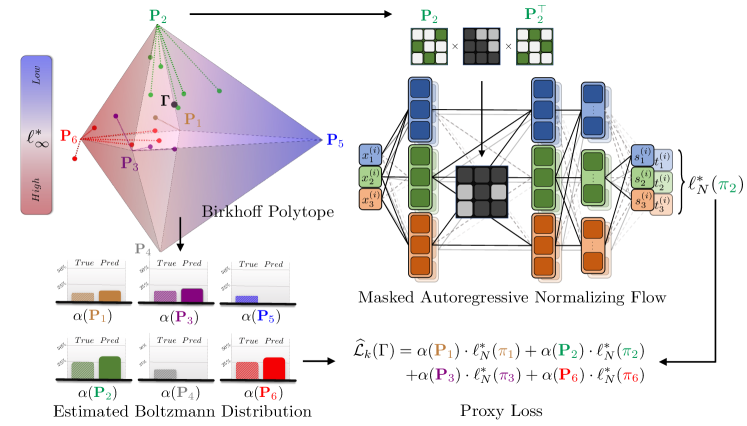
Figure 1: The OCDaf pipeline. The left side shows the permutation learning process on a Birkhoff polytope. We sample permutations from $\mathcal{G}.\mathcal{M}.(\Gamma)$ with parameter $\Gamma$ and use the Gumbel top-k trick to estimate the Boltzmann distribution, shown by $\alpha$. The upper right illustrates how these permutations shape dependencies within the normalizing flow. The calculated proxy loss incorporates the permutation likelihood scores $\ell^{*}_{N}$ and estimated Boltzmann probability $\alpha$.

2 Related Work

We outline previous work on the identifiability of causal directions from observational data and order-based causal structure learning methods. See [33] for a detailed overview of other methods.

Identification of causal directions. Under no assumptions on the form of causal mechanisms, observational data can only identify causal structures up to their Markov equivalence class [12]. Several works have proposed assumptions to identify cause-effect directions. These include restricting causal mechanisms to non-linear models with additive noise [4, 34] or non-Gaussian linear models [35], assuming non-parametric constraints on the variance or conditional entropy of exogenous noises [36, 37, 38, 39, 40] and additional information like non-stationary time-series data [41]. Recent work has demonstrated causal direction identifiability for bivariate causal models with heteroscedastic noises, with noise variances varying across input values [8, 42, 10]. Our work extends these results to the multivariate setting, thus broadening the class of identifiable models.

Ordered-based causal discovery. A part of the structure learning literature has studied searching over the space of topological orderings rather than the super-exponential space of directed acyclic graphs (DAGs) [43, 16, 17, 18, 19, 20, 44]. Some techniques studied include greedy hill-climbing search [21], restricted maximum likelihood estimation (CAM) [15], sparsest permutation [45, 9, 46], and reinforcement learning [47]. While useful, these methods are often combinatorial and do not readily leverage continuous optimization. Recently, the score-matching algorithm (SCORE) has been proposed to find the correct orderings of variables by computing the Hessian of the marginal log-likelihoods of each variable [48, 49]. For Additive Noise Models (ANMs), the Hessian of the leaf nodes is constant. However, this property does not hold for heteroscedastic noise models.

Another direction involves formulating the search over topological orderings as an end-to-end differentiable optimization. BCDNets [50], and VI-DP-DAG [25] model the orderings as latent variables and use variational inference to approximate the posterior over orderings. They formulate orderings as the convex hull of permutation matrices (Birkhoff polytope) and use the Gumbel-Sinkhorn approximation [30] to relax the discrete space of permutations. To calculate the gradients, they either apply the straight-through gradient estimator [51], which involves feeding the hard permutation to the forward pass and using the soft permutation (the result of Sinkhorn) in the backward pass or use the Gumbel-Top-k trick [31]. More recently, Zantedeschi et al. [26] proposed DAGuerreotype that considers parameterizing the permutation vectors by assigning a score to each node, with higher scores indicating higher ranks in the ordering. The SparseMap operator [52] is used to relax their structured search problem and make it differentiable. However, these methods do not offer identifiability results for their derived causal orderings and generally assume their architecture with additive noise during loss calculation.

3 Problem Setup

Data generating model. Suppose we observe $N$ i.i.d. samples from a $d$-dimensional random vector $\mathbf{X}=(X_{1},X_{2},\ldots,X_{d})$. We assume the data is generated from a structural causal model (SCM) $\mathcal{M}=(\mathbf{X},\mathcal{F},P_{\mathbf{U}})$, where each observed variable $X_{i}\in\mathbf{X}$ is a deterministic function of a subset of variables $\mathbf{PA}_{i}\subset\mathbf{X}$ and exogenous noise $U_{i}\sim P_{U_{i}}$:

$$X_{i}=f_{i}(\mathbf{PA}_{i},U_{i}),\;\text{ for some }f_{i}\in\mathcal{F}\quad\forall i\in[d]$$ (1)

where $[d]$ denotes $\{1,\ldots,d\}$. We assume $\mathcal{M}$ satisfies causal minimality, i.e., functions $f_{i}$ are not constant in any of their arguments. The data generating model in Equation (1) induces an observational distribution $P_{\mathcal{M}}$ and a causal directed acyclic graph (DAG) $\mathcal{G}_{\mathcal{M}}$ on $\mathbf{X}$, where $\mathbf{PA}_{i}$ are parents of node $X_{i}$ in the graph. We assume all random variables $X_{i}$ are observed, and exogenous noises $U_{i}$ are zero-mean and mutually independent (Markovian model). We may remove the subscript $\mathcal{M}$ and write $P$ and $\mathcal{G}$ for the observational distribution and the causal DAG, respectively. See Appendix A.1 for a detailed description of the notation and a formal definition of causal minimality.

Identifiability. This work aims to estimate the causal graph $\mathcal{G}_{\mathcal{M}}$ of an SCM $\mathcal{M}$. However, since we only have access to the observational distribution $P_{\mathcal{M}}$, the validity of a graph cannot be generally verified. In particular, we need the causal graph $\mathcal{G}_{\mathcal{M}}$ to be identifiable.

Definition 3.1 (Identifiability).

We call an SCM $\mathcal{M}$ to be structure-identifiable or identifiable if for any SCM $\mathcal{M}^{\prime}\neq\mathcal{M}$ that $P_{\mathcal{M}}=P_{\mathcal{M}^{\prime}}$, we have ${\mathcal{G}_{\mathcal{M}}}={\mathcal{G}_{\mathcal{M}^{\prime}}}$.

Location-scale noise models. It is well-known that identifiability is impossible with no further assumptions on the form of mechanisms $\mathcal{F}$ or exogenous noise $P_{\mathbf{U}}$ [1]. A common approach in the causality literature assumes the exogenous noise is additive, leading to the identifiable class of Additive Noise Models (ANMs) [4]. However, these models generally assume the noise variance to be constant. A more general notion of ANMs, known as location-scale noise models, considers heteroscedastic noise that can depend on the value of parents [8, 42, 10]:

Definition 3.2.

(LSNMs) A SCM $\mathcal{M}$ is called Location-Scale Noise-Model (LSNM) if it has the following form

$$X_{i}=f_{i}(\mathbf{PA}_{i})+g_{i}(\mathbf{PA}_{i})\cdot U_{i}$$ (2)

where $f_{i},g_{i}:\mathbb{R}^{|\mathbf{PA}_{i}|}\to\mathbb{R}$ are twice-differentiable w.r.t. each input argument, and $g_{i}>0$.

This paper proves the identifiability of causal graphs in multivariate LSNMs and provides a structure learning algorithm. We follow a two-stage procedure similar to Bühlmann et al. [15], where we first learn a valid topological ordering of the causal DAG and then prune the spurious edges. Our learning algorithm leverages the class of autoregressive normalizing flows to estimate valid orderings. A valid (topological) ordering of a DAG $\mathcal{G}$ is a permutation $\pi$ of $[d]$ such that for any pair $X_{i}$ that causally precedes $X_{j}$, $\pi(i)<\pi(j)$. We denote the set of all valid orderings of a DAG $\mathcal{G}$ as $\Pi_{\mathcal{G}}$ or simply $\Pi$.

Autoregressive normalizing flows. Normalizing flows [29] are a class of deep generative models that express a given probability distribution through a series of transformations. The goal of normalizing flows is to learn a diffeomorphism $\mathbf{T}:\mathbb{R}^{d}\to\mathbb{R}^{d}$ that maps $\mathbf{X}$ to a base distribution $P_{\mathbf{U}}(\cdot)$. The density of $\mathbf{X}$ can be obtained via the change of variables formula ($\mathbf{J}$ is the Jacobian matrix of $\mathbf{T}$):

$$P_{\mathbf{X}}(\mathbf{x})=P_{\mathbf{U}}(\mathbf{T}(\mathbf{x}))\cdot\left|\det\mathbf{J}_{\mathbf{T}}(\mathbf{x})\right|$$ (3)

Autoregressive normalizing flows (ANFs) [28] impose an autoregressive structure on the transformation $\mathbf{T}$ making the Jacobian determinant lower-triangular and simplifying the likelihood computation. Specifically, the transformation decomposes into a series of $d$ one-dimensional mappings:

$$u_{i}=T_{i}(x_{i}\mid\mathbf{x}_{<\pi(i)}),\quad\forall i\in[d],$$ (4)

where $\pi$ is a permutation that specifies the ordering of the autoregressive structure, $\mathbf{x}_{<\pi(i)}$ denotes the vector of the first $i-1$ components of $\mathbf{x}$ w.r.t. $\pi$, and $T_{i}$ is a one-dimensional mapping that is invertible w.r.t. $x_{i}$ and is parameterized by the condition $\mathbf{x}_{<\pi(i)}$.

Permutation Learning. Searching over the space of orderings can be formulated as a search over the discrete space of all $d\times d$ permutation matrices denoted by $\mathcal{P}_{d}$. However, finding a valid permutation in such space becomes intractable as $d$ goes large since $|\mathcal{P}_{d}|=d!$. A common practice is parameterizing $\mathcal{P}_{d}$ with a continuous parameter $\Gamma$, where each permutation $\mathbf{P}\in\mathcal{P}_{d}$ is represented using the matching operator that maximizes the Frobenius inner product between matrices:

$$M(\Gamma):=\operatorname*{arg\,max}_{\mathbf{P}\in\mathcal{P}_{d}}\langle\mathbf{P},\Gamma\rangle_{F}\quad$$ (5)

Due to the non-differentiability of the matching operator, previous works have proposed a differentiable approximation called the Sinkhorn operator $S(\Gamma/\tau)$ with an infinitesimal temperature $\tau$ [30]. Additionally, some works learn a distribution over the permutations. For example, the Gumbel Matching distribution $M(\Gamma+\epsilon)\sim\mathcal{G}.\mathcal{M}.(\Gamma)$ is generated by sampling $\epsilon$ — a matrix of standard i.i.d. Gumbel noise. This distribution is closely linked to the parameterized Boltzmann distribution over permutations, where the energy of a permutation $\mathbf{P}\in\mathcal{P}_{n}$ is equal to $\langle\Gamma,\mathbf{P}\rangle_{F}$. As illustrated heuristically in [53, 54], the Gumbel-Matching distribution is capable of yielding approximate or unbiased samples from the true density.

4 Discovering Causal Graphs in Multivariate LSNMs

4.1 Identification of Causal Graphs

Prior research has confirmed the identifiability of LSNMs within a bivariate setting. A common approach in finding all non-identifiable scenarios for these constrained SCMs involves deriving a differential equation that holds for both causal and anti-causal directions. Immer et al. [10] achieved this for LSNMs. However, their condition does not easily extend to scenarios involving more than two variables. Directly extrapolating their proof involves checking the bivariate condition for all parent-child pairs while fixing the value of other parents; however, this fails in the context of ANMs [4]. This section focuses on the identifiability results in multivariate settings. Given the technical nature of the proof, we present only the final result here, deferring the detailed proof to Appendix A. A similar expansion from bivariate to multivariate settings has been previously established in the domain of restricted ANMs by Peters et al. [4]. To avoid intricacies, we focus solely on a specific subclass of non-linear LSNMs with Gaussian noise within the main text. For this model class, all solutions to the aforementioned differential equation have been characterized in the bivariate setting by Khemakhem et al. [8]. We present and prove the more general case in  Appendix A.

Definition 4.1 (GI-LSNM).

Consider an LSNM Definition (3.2) and the following conditions:

1. $\{U_{i}\}_{i=1}^{d}$ follow standard Gaussian independent of all $X_{j}\in\mathbf{PA}_{i}$.

2. For each $X_{i}$ and each $X_{j}\in\mathbf{PA}_{i}$, there is at least one value of $\mathbf{x}_{\mathbf{PA}_{i}\backslash\{X_{j}\}}$ with positive probability, such that $f_{i}(\mathbf{x}_{\mathbf{PA}_{i}\backslash\{X_{j}\}},{\cdot})$ is a non-linear & invertible function of $X_{j}$.

We denote an LSNM that satisfies the first condition as Gaussian LSNM and a model that satisfies both conditions as Gaussian Invertible LSNM (GI-LSNM).

Theorem 4.1.

GI-LSNMs are identifiable: For any GI-LSNMs $\mathcal{M}$ and any Gaussian LSNM $\mathcal{M}^{\prime}$ that $P_{\mathcal{M}^{\prime}}=P_{\mathcal{M}}$, we have ${\mathcal{G}_{\mathcal{M}}}={\mathcal{G}_{\mathcal{M}^{\prime}}}$.

Theorem 4.1 does not limit other LSNMs with the same observational distribution to be non-linear invertible. As demonstrated in subsection 4.2, this allows us to employ a broader class of LSNM when learning the correct ordering. We also note that the choice of standard Gaussian noise is not necessary for identifiability, as we state in  Appendix A. For non-Gaussian noises, however, characterizing all the identifiable cases in closed form is an open direction, which we leave as future work.

4.2 LSNMs as Autoregressive Normalizing Flows

In the previous section, we established that GI-LSNMs are structure-identifiable. The next challenge is to devise a suitable method for estimating causal graphs. As discussed earlier, we follow a two-stage learning algorithm, where we first estimate a valid causal ordering over the variables and then apply an additional pruning step to get the final graph. While the likelihood-ratio testing proposed by Immer et al. [10] effectively estimates the correct causal direction in bivariate settings, extending this approach to multivariate data is not straightforward. As we discuss in  Appendix B, the relationship between pairs of parent-child nodes in a multivariate LSNM does not necessarily follow a bivariate LSNM, rendering the bivariate likelihood ratio test unable to identify the correct direction by checking all the pairs of nodes. Instead, we derive a multivariate likelihood ratio test on the full data while ensuring our parametric model follows an LSNM structure. We choose autoregressive normalizing flows (ANFs) as our parametric model. As discussed in Khemakhem et al. [8], restricting the transformer functions within ANFs to affine functions exhibit a similar form to LSNMs:

Definition 4.2 (Affine ANFs).

Given a permutation $\pi$ of $[d]$ and a random vector $\mathbf{X}\in\mathbb{R}^{d}$, an affine ANF parameterized by $\Theta$ is an autoregressive normalizing flow, where its transformations $T_{i}$ are expressed as follows:

$$T^{\theta}_{i}(x_{i}|\mathbf{x}_{<\pi(i)})=\frac{x_{i}-t_{i}^{\theta}(\mathbf{x}_{<\pi(i)})}{\exp\left(s_{i}^{\theta}(\mathbf{x}_{<\pi(i)})\right)}\quad\forall i\in[d]$$ (6)

The functions $t^{\theta}_{i},s^{\theta}_{i}$ are twice differentiable for $\theta\in\Theta$. We also assume that $\Theta$ is expressive, i.e., for any twice differentiable functions $\{t_{i},s_{i}\}_{i=1}^{d}$, there exists $\theta$ such that $t^{\theta}_{i}=t_{i},\ s^{\theta}_{i}=s_{i}$. 

The similarity between affine ANFs and LSNMs stems from the fact that once trained, the transformations $T_{i}$ generate independent base distributions $U_{i}$ (e.g., Gaussian). Therefore, we can reverse Equation (6) and write $X_{i}$ as a function of previous variables $\mathbf{X}_{<\pi(i)}$ and independent noise $U_{i}$. This can be correspondingly mapped to LSNMs in Equation (2):

$$X_{i} =t_{i}^{\theta}(\mathbf{X}_{<\pi(i)})\ + \ \exp\left(s_{i}^{\theta}(\mathbf{X}_{<\pi(i)})\right) \cdot U_{i}~{}$$ (7)

$$X_{i} =f_{i}(\mathbf{PA}_{i})\ + \ g_{i}(\mathbf{PA}_{i}) \cdot U_{i}$$ (LSNM)

The difference is that, in Equation (7), $X_{i}$ is a function of all previous nodes $\mathbf{X}_{<\pi(i)}$ while it only depends on its parent nodes $\mathbf{PA}_{i}$ in LSNMs. Nonetheless, by parameterizing affine ANF with expressive multi-layer perceptrons (MLPs), $s^{\theta}_{i}$ and $t^{\theta}_{i}$ can be constant w.r.t. any subset of their inputs $\mathbf{X}_{<\pi(i)}$. Consequently, our model in Equation (7) includes LSNMs. 

Given an ordering $\pi$, we can then use the change of variables formula in Equation (3) to express the log-likelihood of $\mathbf{X}$ under the parametric choice of affine ANFs with $P_{U}$ as base distribution. We choose $P_{U}$ as a standard Gaussian distribution. However, it should be noted that any choice of base distribution can be employed given the prior belief about the noise model. Given a dataset $\mathcal{D}=\{\mathbf{x}^{(i)}\}_{i=1}^{N}$, we consider the following procedure to find a valid causal ordering. For each ordering $\pi$, we estimate the maximum expected log-likelihood of the data as follows:

$$\ell^{*}_{N}(\pi):=\max_{\theta\in\Theta}\ell_{N}(\pi;\theta)\text{, where }\ell_{N}(\pi;\theta):=\frac{1}{N}\sum_{i=1}^{N}\log P_{\mathbf{X}}(\mathbf{x}^{(i)};\pi,\theta)$$ (8)

In an infinite sample setting, selecting the ordering with the highest maximum expected log-likelihood ensures a valid ordering. See  Appendix C for the proof.

Proposition 4.2.

Consider a GI-LSNM $\mathcal{M}$ from Definition 4.1, and $\Theta$ as the parametric affine ANF in Definition 4.2. For each permutation $\pi$, let $\ell^{*}_{\infty}(\pi)$ be the maximum expected log-likelihood under this model. That is,

$$\ell^{*}_{\infty}(\pi):=\max_{\theta\in\Theta}\mathbb{E}_{\mathbf{x}\sim P_{\mathcal{M}}}\left[\log P_{\mathbf{X}}(\mathbf{x};\pi,\theta)\right]$$ (9)

Then, $\forall\pi\in\Pi_{\mathcal{G}_{\mathcal{M}}},\pi^{\prime}\not\in\Pi_{\mathcal{G}_{\mathcal{M}}}$, it holds that $\ell^{*}_{\infty}(\pi)>\ell^{*}_{\infty}(\pi^{\prime})$. In other words, the expected log-likelihood of all valid orderings is strictly greater than those of other orderings.

4.3 Finite-Sample Estimation of Causal Ordering

This section focuses on the learning algorithm for obtaining a valid causal ordering in finite samples. The previous section described our procedure as finding an ordering $\pi$ that maximizes $\ell^{*}_{N}(\pi)$. However, the space of all orderings is a discrete set that grows super-exponentially w.r.t. $d$. Even for moderate $d$, solving this problem becomes computationally intractable and non-differentiable, rendering standard optimization techniques used in deep learning ineffective.

Instead of direct optimization over orderings, we treat each ordering $\pi$ as a permutation over the covariates, characterized by permutation matrix $\mathbf{P}_{\pi}$, and consider a differentiable proxy loss based on a Boltzmann distribution parameterized by $\Gamma$:

$$\mathcal{L}(\Gamma)=\sum_{\mathbf{P}_{\pi}\in\mathcal{P}_{d}}\alpha(\mathbf{P}_{\pi})\cdot\ell^{*}_{N}(\pi)\quad\text{with}\quad\alpha(\mathbf{P}_{\pi})=\frac{\exp{\langle\Gamma\cdot\mathbf{P}_{\pi}\rangle_{F}}}{Z(\Gamma)}$$ (10)

where $Z(\Gamma)=\sum_{\mathbf{P}^{\prime}\in\mathcal{P}_{d}}\exp{\langle\Gamma\cdot\mathbf{P}^{\prime}\rangle_{F}}$ is the partition function. Figure 1 demonstrates how the proxy loss weights permutation matrices based on their Euclidean distance from $\Gamma$. Since $\Gamma$ is not bounded, the Boltzmann distribution can degenerate on any permutation. Hence, in principle, it can converge to the permutation with maximum $\ell^{*}_{N}(\pi)$.

The proxy loss in Equation (10) solves the differentiability problem. However, the intractability issue remains as the partition function requires summing over all $d!$ permutations. As discussed in section 3, a common approach to avoid calculating the partition function is to approximate the above Boltzmann distribution using the Gumbel-Matching distribution $\mathcal{G}.\mathcal{M}.(\Gamma)$:

$$\mathcal{L}(\Gamma)\approx\mathbb{E}_{\mathbf{P}_{\pi}\sim\mathcal{G}.\mathcal{M}.(\Gamma)}\left[\ell^{*}_{N}(\pi)\right]$$ (11)

Although the Gumbel-Matching distribution provides a tractable approximation, it is not differentiable w.r.t. $\Gamma$. One approach suggested in the literature involves approximating the Gumbel-Matching distribution using the differentiable Gumbel-Sinkhorn operator with low temperature to generate ”soft” permutation matrices [30]. In practice, the likelihood function $P_{\mathbf{X}}(\cdot;\pi,\theta)$ is defined w.r.t. the ”hard” permutations $\mathbf{P}_{\pi}$. Therefore, the optimization often involves employing a straight-through gradient estimator [51] that applies the matching operator to generate hard permutations in the forward pass while passing the gradients through the differentiable Sinkhorn operator in the backward pass [50, 25]. Instead of using the Sinkhorn operator, Charpentier et al. [25] propose an alternative approach based on the Gumbel-Top-k trick [31] that directly samples from the Gumbel-Matching distribution and use the generated samples to approximate the Boltzmann distribution. In particular, assume we draw $k$ independent samples $\mathcal{H}_{k}=\{\mathbf{P}^{(1)},\ldots,\mathbf{P}^{(k)}\}$ without replacement from $\mathcal{G}.\mathcal{M}.$ The approximated proxy loss function is as follows:

$$\hat{\mathcal{L}}_{k}(\Gamma):=\frac{\sum_{\mathbf{P}_{\pi}\in\mathcal{H}_{k}}\exp{\langle\Gamma,\mathbf{P}_{\pi}\rangle_{F}}\cdot\ell^{*}_{N}(\pi)}{\sum_{\mathbf{P}_{\pi^{\prime}}\in\mathcal{H}_{k}}\exp{\langle\Gamma,\mathbf{P}_{\pi^{\prime}}\rangle_{F}}}$$ (12)

In our experiments, we evaluate our method using both Gumbel-Sinkhorn and Gumbel-Top-k tricks. In practice, we concurrently optimize the ANF model parameters $\theta$ and permutation parameters $\Gamma$ using alternating optimization to $\ell^{*}_{N}(\pi)$. At the end of the training, the most frequently generated permutation is considered as the correct ordering. We present the algorithm details in  Appendix D.

Network architecture. Up to this point, we have written the proxy loss $\mathcal{L}$ as a function of $\Gamma$ and $\ell_{N}$, where the latter depends on functions $\{t^{\theta}_{i},s^{\theta}_{i}\}_{i=1}^{d}$. Here, we briefly explain the network architecture of functions $t_{i}$ and $s_{i}$. Instead of the naive approach of using $2d$ different MLPs for each dimension, we utilize masked MLPs and employ a single neural network with shared parameters to predict all $t_{i}$ and $s_{i}$ together, inspired by masked autoregressive flows for density estimation [55],

Since our goal is to search over different permutation matrices, we formulate our architecture using arbitrary permutation matrices $\mathbf{P}$. The MLP architecture can be concisely described by the following set of equations:

$$h^{(l+1)}=\begin{cases}\sigma([\mathbf{P}L\mathbf{P}^{\top}\circ W^{(l)}]\cdot h^{(l)})&\text{if }l+1\neq k\\ \sigma([\mathbf{P}\hat{L}\mathbf{P}^{\top}\circ W^{(l)}]\cdot h^{(l)})&\text{o.w.}\end{cases},\text{where }\begin{cases}L_{i,j}=\mathbb{I}(i\leq j)\\ \hat{L}_{i,j}=\mathbb{I}(i<j)\end{cases}$$ (13)

where $h^{(l)}$ is the output of the $l^{\text{th}}$ hidden layer and $k$ is the number of layers. This architecture enables the model to handle multiple permutations simultaneously and facilitates parameter sharing between different permutations, maximizing network utilization during order discovery. The lower-triangular mask matrix $L$ ensures that the output for the $i^{th}$ covariate depends only on preceding covariates in the specified permutation $\mathbf{P}\in\mathcal{P}_{n}$. For ease of notation, we have assumed that $h^{(l)}$ are all $d$-dimensional. However, we use blocked matrix multiplication operations in the final model. See Appendix E for a detailed explanation of our architecture.

5 Experiments

The objectives of our experiments are as follows. First, we evaluate our method on the standard real-world benchmarks such as the Sachs dataset [2] and SynTReN [32] and show the state-of-the-art performance w.r.t. the structural hamming distance (SHD) and structural intervention distance (SID), making heteroscedastic noise models a better choice than the more frequently-used additive noise models (ANMs). We then aim to empirically validate our theoretical findings that OCDaf  successfully identifies the correct causal orderings in correctly-specified models. We show our method’s robust performance under both real-world and synthetically generated data. Finally, we provide empirical evidence that causal ordering, without additional pruning, can consistently estimate interventional distributions. The following briefly describes the datasets, baselines, and evaluation metrics. See Appendix G for a detailed description of our experiments and the hyperparameters.

Dataset. We evaluate OCDaf on a diverse array of real-world, synthetic, and pseudo-real datasets. These include the Sachs dataset [2] with $N=853$ observations and $d=11$ proteins from human immune system cells, and $10$ datasets from SynTReN [32], each comprising $N=500$ simulated gene expressions and $d=20$ nodes with $20$ to $25$ edges. We further include a comprehensive benchmark of various sized DAGs with different causal structures, generated using both linear and non-linear processes. These include Gaussian processes [56] for non-parametric non-linear formats, alongside parametric schemes with additive and heteroscedastic noise models. To assess model misspecification, we incorporate both Gaussian and Laplace exogenous noises. This benchmark offers a robust testing environment for causal discovery. For additional details, see Appendix F.

Baselines and Comparative Methods. In our evaluation of orderings, we consider methods that initially learn a causal ordering and then prune the resulting full DAG. We benchmark our algorithm against several state-of-the-art methods, including CAM [15], DAGuerreo [26], SCORE [48], and VI-DP-DAG [25]. These methods assume additive noise models. Additionally, we employ the estimator proposed by Immer et al. [10] for bivariate location-scale noise models (bi-LSNM), adapting it to our multivariate setting. For each pair of nodes, we apply their method and rank the nodes based on pairwise comparisons. In line with Reisach et al. [57], simulated data can sometimes allow for topological orderings to be estimated simply by sorting variables based on their marginal variance. Therefore, we include the VarianceSort baseline in our comparisons. Furthermore, we compare our algorithm to models that directly learn DAGs without explicit permutation learning. We achieve this by applying an additional pruning step to our estimated permutation. Notably, we also compare our results against GraN-DAG [23] on real-world datasets. GraN-DAG is a continuous likelihood-based method that directly learns the causal graph structure and has achieved state-of-the-art results on the aforementioned real-world data.

Evaluation Metrics. Regarding learning valid causal orderings, we propose a metric called causal backward count (CBC). This metric utilizes the concordance index on the set of causal pairs. The CBC metric lets us compare the derived ordering $\hat{\pi}$ with the correct causal graph’s ordering $\mathcal{G}$. It is calculated using the formula $\text{CBC}_{\mathcal{G}}(\hat{\pi})=\sum_{(i,j)\in E(\mathcal{G})}\mathbb{I}(\hat{\pi}(i)>\hat{\pi}(j))/|E(\mathcal{G})|,$ where $E(\mathcal{G})$ represents the edges in the causal graph and $\mathbb{I}(\cdot)$ is an indicator function. After applying various pruning techniques to derive a causal graph $\hat{\mathcal{G}}$, we evaluate the learned graph using established metrics for DAG learning, namely the Structural Hamming Distance (SHD) and the Structural Intervention Distance (SID) [58]. The SHD metric serves to quantify the dissimilarity between the $\hat{\mathcal{G}}$ and $\mathcal{G}$ by measuring the number of necessary modifications, including additions, removals, and reversals of edges, required to transform the estimated DAG into the true one. On the other hand, the SID metric calculates the similarity between two DAGs in terms of their corresponding causal inference statements. It achieves this by counting the number of disrupted causal paths in $\hat{\mathcal{G}}$.

Table 1: Comparison of OCDaf with baselines on Sachs and SynTReN datasets using CBC, SHD, and SID metrics (¹ used the Gumbel-Sinkhorn, ² used the Gumbel-Top-k approach, ^a used PC-KCI for pruning, ^b used the sparse-regression technique for pruning). 

Sachs SynTReN CBC SHD SID Avg CBC SHD SID OCDaf (Top-k)^a 0.18 $\pm$ 0.11 10.4 $\pm$ 0.89 46.4 $\pm$ 6.77 0.21 $\pm$ 0.17 32.0 $\pm$ 2.9 161.0 $\pm$ 58.9 OCDaf (Top-k)^b 0.18 $\pm$ 0.11 10.4 $\pm$ 0.89 46.4 $\pm$ 6.77 0.21 $\pm$ 0.17 34.3 $\pm$ 3.4 122.9 $\pm$ 57.1 CAM 0.41 12 55 0.33 $\pm$ 0.14 41.7 $\pm$ 7.1 139.6 $\pm$ 36.1 SCORE 0.47 12 45 0.38 $\pm$ 0.10 37.5 $\pm$ 4.4 197.1 $\pm$ 67.1 VarSort 0.47 12 45 0.51 $\pm$ 0.21 46 $\pm$ 9.9 187.4 $\pm$ 81.1 DAGuerreo 0.13 $\pm$ 0.03 20.4 $\pm$ 0.9 48.8 $\pm$ 2.1 0.40 $\pm$ 0.16 74.1 $\pm$ 11.5 159.4 $\pm$ 69.4 VI-DP-DAG¹ 0.34 $\pm$ 0.11 29 $\pm$ 1.8 46.2 $\pm$ 3.3 0.6 $\pm$ 0.21 142.1 $\pm$ 8.5 147.1 $\pm$ 36.8 VI-DP-DAG² 0.48 $\pm$ 0.12 33 $\pm$ 2.9 41.6 $\pm$ 6.2 0.58 $\pm$ 0.17 137.2 $\pm$ 9.4 152.6 $\pm$ 40.4 bi-LSNM 0.59 19 59 0.46 $\pm$ 0.17 49.5 $\pm$ 7.6 170.1 $\pm$ 75.6 GraN-DAG - 13 47 - 34.0 $\pm$ 8.5 161.7 $\pm$ 53.4 PC - 17 [47, 62] - 41.2 $\pm$ 5.1 [154.8 $\pm$ 47.6, 179.3 $\pm$ 55.6]

Real-world and semi-synthetic. Table 1 presents a comparative analysis of our method, OCDaf, with other baseline methods on the Sachs and SynTReN datasets, employing different evaluation metrics. Using sparse regression and PC with Kernel-based conditional independence test pruning techniques as introduced by [15] and [59] respectively, OCDaf surpasses most baselines in terms of CBC, SHD, and SID on the Sachs dataset, achieving state-of-the-art results for SHD. To account for any randomness in our results for the Sachs dataset, the standard deviation and average of the metrics were calculated across multiple runs of OCDaf using various seeds. Furthermore, on the SynTReN dataset, OCDaf outperforms many baselines in CBC and SHD metrics, demonstrating its versatility when combined with different pruning techniques. For the method DAGuerreo, we were unable to reproduce the exact reported metrics; therefore, we tested it on both standardized and non-standardized versions of the dataset, and the version with the lowest CBC was reported. For further details on baseline implementations, refer to Appendix G.

Synthetic benchmark. Table 2 compares OCDaf with other baseline approaches on a synthetic dataset using the CBC metric. Our method is evaluated using both Gumbel-Top-k and Gumbel-Sinkhorn sampling techniques. Notably, all synthetic experiments conducted were standardized to a zero mean with a variance of one. Although this standardization does not alter the class of data (ANM or LSNM), it effectively prevents trivial solutions such as variance sorting [33]. As a sanity check, we note that all models perform comparably and poorly on the non-identifiable linear Gaussian case, as expected. Our method provides flexibility in the choice of the base distribution for calculating likelihood. Therefore, we also evaluate it on linear data with Laplace exogenous noise. We assess our method under two different conditions: the correctly specified base distribution and the default Gaussian noise. OCDaf (Gumbel-Top-k) surpasses other baselines under the correctly-specified noise distribution, even though the linear models with Laplace noise do not conform to GI-LSNM. Conversely, its performance declines under noise misspecification, indicating the sensitivity of our model to the specific definition of the likelihood model. Lastly, we shift our focus to nonparametric and nonlinear parametric datasets. As anticipated, all baseline models that assume additive noise perform better in additive settings. However, their result considerably drops in the affine heteroscedastic noise, showing their sensitivity to the heteroscedasticity of the noise. Contrarily, our model demonstrates consistent performance in both additive and affine settings and surpasses other baselines, with the exception of CAM and SCORE, which excel in the additive case. Finally, for testing the model scalability, we have included a similar comparison of OCDaf and baselines on larger graphs with $d\in\{10,25\}$ in Appendix F.

Table 2: Comparison of CBC metric (mean $\pm$ standard deviation) for different graph structures (chain, full-graph, Erdős–Rényi) and different seeds. We benchmarked OCDaf with Gumbel-Sinkhorn and Gumbel-Top-$k$ on small datasets with $d\in{3,4,5,6}$ (^∗ datasets utilized Laplace instead of Gaussian base distribution).

	Linear	Linear Laplace		Nonparametric		Nonlinear Parametric
	Gaussian	Affine	Additive	Affine	Additive	Affine	Additive
OCDaf (Top-k)	$0.46\pm 0.27$	$0.83\pm 0.17$ ($\mathbf{0.22\pm 0.20}$)∗	$0.7\pm 0.2$ ($\mathbf{0.16\pm 0.18}$)∗	$\mathbf{0.12\pm 0.14}$	$\mathbf{0.13\pm 0.15}$	$\mathbf{0.15\pm 0.18}$	$\mathbf{0.20\pm 0.19}$
OCDaf (Sinkhorn)	$0.48\pm 0.28$	$0.81\pm 0.28$ ($0.42\pm 0.28$)∗	$0.69\pm 0.29$ ($0.46\pm 0.30$)∗	$0.29\pm 0.22$	$0.37\pm 0.29$	$0.38\pm 0.24$	$0.42\pm 0.28$
CAM	$0.44\pm 0.34$	$0.86\pm 0.19$	$0.67\pm 0.38$	$0.27\pm 0.25$	$\mathbf{0.02\pm 0.07}$	$0.83\pm 0.27$	$\mathbf{0.19\pm 0.25}$
VI-DP-DAG	$0.59\pm 0.34$	$0.67\pm 0.3$	$\mathbf{0.4\pm 0.28}$	$0.42\pm 0.25$	$0.42\pm 0.26$	$\mathbf{0.65\pm 0.23}$	$0.51\pm 0.25$
DAGuerreo	$0.4\pm 0.28$	$0.81\pm 0.21$	$0.5\pm 0.32$	$0.27\pm 0.22$	$0.14\pm 0.19$	$0.74\pm 0.31$	$0.44\pm 0.30$
SCORE	$0.53\pm 0.29$	$0.68\pm 0.31$	$0.73\pm 0.3$	$\mathbf{0.1\pm 0.17}$	$\mathbf{0.00\pm 0.00}$	$0.78\pm 0.35$	$0.44\pm 0.40$
VarSort	$0.39\pm 0.16$	$\mathbf{0.52\pm 0.24}$	$0.47\pm 0.23$	$0.36\pm 0.25$	$0.17\pm 0.19$	$0.66\pm 0.43$	$0.49\pm 0.37$
biLSNM	$0.54\pm 0.22$	$0.59\pm 0.19$	$0.56\pm 0.17$	$0.56\pm 0.21$	$0.56\pm 0.21$	$\mathbf{0.57\pm 0.22}$	$0.57\pm 0.22$

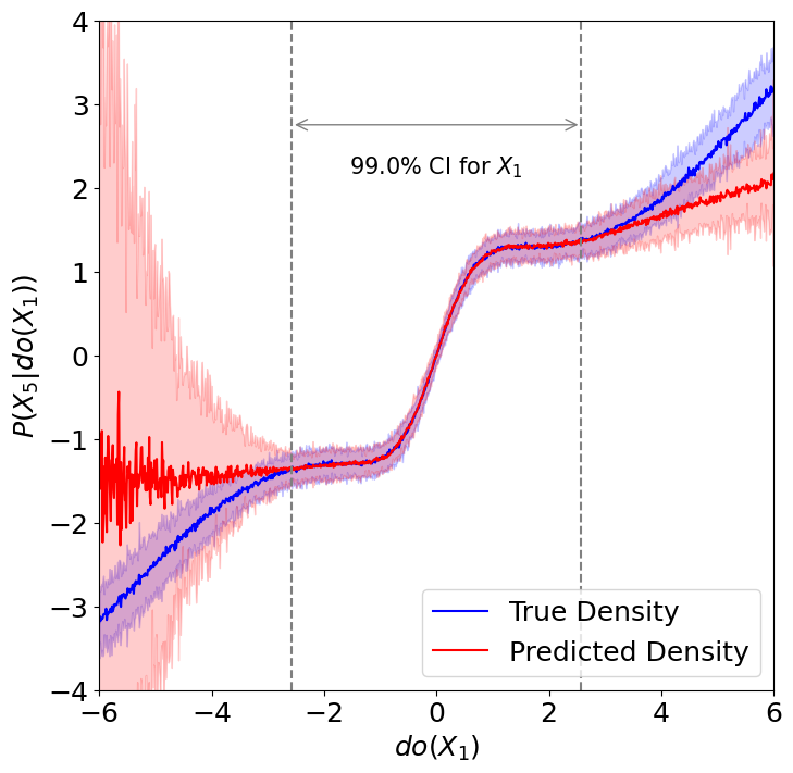
Figure 2: Accurate interventional distribution prediction in a causal chain with $X_{1}$ and $X_{5}$ being the first and last nodes.

Interventions. The causal ordering of a data-generating process is sufficient for estimating the corresponding interventional distributions in infinite samples [15]. Here, we consider estimating the interventional effects from finite samples. Initially tested in bivariate settings by [8], we extended it to a multivariate case. Following a similar procedure, we generate observational samples from an LSNM and train OCDaf on it. We then use a similar procedure by Khemakhem et al. [8] to generate interventional data from the learned model and compare it to the ground-truth interventions. Figure 2 shows an example with five nodes, where $P(X_{5}|do(X_{1}))$ is estimated. Notably, as $X_{1}$ values are pushed beyond the observational domain, the predicted distribution error progressively increases. See Appendix H for the details of the data-generating process and additional experimental results.

6 Conclusion & Limitations

This paper presents proof of the identifiability of multivariate heteroscedastic noise models with observational data. Drawing on these theoretical findings, we introduce OCDaf , a novel algorithm designed to accurately estimate valid causal orderings. Our theory is evaluated by a comprehensive series of synthetic experiments, and we demonstrate state-of-the-art performance in the standard Sachs and SynTReN benchmarks. While our main theoretical results primarily focus on the class of invertible Gaussian noise models, we present a general identifiability theory in our appendix. Nonetheless, the task of characterizing identifiable models with other noise distributions remains an open challenge, providing an intriguing direction for subsequent research.

Limitations and future work: The practical efficacy of our method, however, comes with some limitations. Notably, our method exhibits a longer overall running time compared to other baselines, which was observed during our experiments. While there are avenues to improve the performance of the algorithm, we posit that fundamentally new ideas will be required to scale up such methods to hundreds of thousands of variables – a fertile direction for future work. Moreover, we mainly compare our methods to those that explicitly identify topological orders – with the exception of GraN-DAG. To the best of our knowledge, no other work has reported superior SHD and SID metrics for the Sachs dataset, yet a more comprehensive comparison of using OCDaf in conjunction with pruning-based methods against an expanded set of baselines in both synthetic and real-world scenarios will provide a more robust assessment of OCDaf ’s performance.

Appendix A Proof of Theorem 4.1

This section aims to prove Theorem 4.1 for a general class of LSNMs, including GI-LSNM. We first re-state the identifiability results for bivariate LSNMs from Immer et al. [10]. As we mentioned in Section 4.1, this bivariate condition does not readily extend to the multivariate setting. Therefore, we define a sub-class of multivariate LSNMs, called ”restricted” LSNMs, in which the bivariate condition is satisfied for all pairs of child-parent nodes. We then show identifiability under this class of models. The notion of restricted LSNMs is analogous to restricted ANMs proposed by Peters et al. [4], and our proof largely employs similar techniques. Finally, we show that GI-LSNMs belong to the class of restricted LSNMs, concluding our proof.

A.1 Notation

We use uppercase letters for random variables and lowercase letters for a realization of them. Vectors and sets are shown with bold symbols. The density function of a random variable $X$ is denoted as $P_{X}$, or simply $P$. Given an SCM $\mathcal{M}=(\mathbf{X},\mathcal{F},P_{\mathbf{U}})$, $\mathbf{PA}^{\mathcal{M}}_{i}$ and $\mathbf{ND}^{\mathcal{M}}_{i}$ refer to the set of parent nodes and non-descendent nodes of a random variable $X_{i}\in\mathbf{X}$ in the corresponding causal graph $\mathcal{G}_{\mathcal{M}}$, respectively. We may remove superscript $\mathcal{M}$ and write $\mathbf{PA}_{i}$ and $\mathbf{ND}_{i}$. For a multivariate function $f(Z_{1},\ldots,Z_{m})$, we use $f\big{|}_{\mathbf{S}=\mathbf{s}}$ to fix input arguments for every $Z_{i}\in\mathbf{S}$ to their corresponding value in $\mathbf{s}$. Finally, for random variables $X$ and $Y$ we use $X\big{|}_{Y=y}$ to denote the random variable $X$ after conditioning on $Y=y$.

Before starting the proof, we formally define causal minimality for a structural causal model (SCMs).

Definition A.1 (Causal Minimality).

A SCM $\mathcal{M}=(\mathbf{X},\mathcal{F},P_{\mathbf{U}})$ satisfies causal minimality if all its mechanisms $f_{i}\in\mathcal{F}$ are not constant in any of their arguments, i.e., for any $X_{i}$ and $X_{j}\in\mathbf{PA}_{i}$, there are some $\mathbf{x}_{\mathbf{PA}_{i}\backslash{\{X_{j}\}}}$ and some $x_{j}\neq x^{\prime}_{j}$ such that

$$f_{i}(\mathbf{x}_{\mathbf{PA}_{i}\backslash{\{X_{j}\}}},x_{j})\neq f_{i}(\mathbf{x}_{\mathbf{PA}_{i}\backslash{\{X_{j}\}}},x^{\prime}_{j})$$

A.2 Bivariate identifiability

We first define an abstract notion of bivariate identifiability that will be used throughout the proof.

Definition A.2 (bivariate identifiability).

Consider a tuple $\left(f,g,p_{X}(X),p_{U}(U)\right)$ with twice differentiable functions $f$ and $g>0$ on $\mathbb{R}$, and independent random variables $U$ and $X$. Define

$$Y=f(X)+g(X)\cdot U$$

We call the tuple bivariate identifiable if there are no twice differentiable functions $h,k:\mathbb{R}\to\mathbb{R}$ (with $k>0$), such that the backward model holds:

$$X=h(Y)+k(Y)\cdot V\ \text{ for some $V\perp\!\!\!\perp Y$ with $p_{V}=p_{U}$.}$$

In particular, Khemakhem et al. [8] characterize the bivariate identifiability for the case of Gaussian exogenous noise, and Immer et al. [10] propose a sufficient condition for general noise by deriving a differential equation that must hold for both causal and anti-causal directions:

Theorem A.1 (Khemakhem et al. [8]).

Consider random variables $X$ and $Y$, where their joint distribution $P(X,Y)$ can be induced by LSNMs with both directions, i.e.,

$$Y=f(X)+g(X)\cdot U,\quad U\perp\!\!\!\perp X$$

$$X=h(Y)+k(Y)\cdot V,\quad V\perp\!\!\!\perp Y$$

for Gaussian variables $U,V$, and twice differentiable functions $f,g,h,k$ on $\mathbb{R}$, where $g,k>0$. Then one of the following scenarios must hold:

1. $(g,f)=\left(\frac{1}{\sqrt{Q}},\frac{P}{Q}\right)$ and $(k,h)=\left(\frac{1}{\sqrt{Q^{\prime}}},\frac{P^{\prime}}{Q^{\prime}}\right)$ where $Q,Q^{\prime}$ are polynomials of degree two, $Q,Q^{\prime}>0$, $P,P^{\prime}$ are polynomials of degree two or less, and $p_{X},p_{Y}$ are strictly log-mix-rational-log. In particular, $\lim_{-\infty}g=\lim_{+\infty}g=0^{+}$, $\lim_{-\infty}f=\lim_{+\infty}f<\infty$, similarly so for $k,h$, and $f,g,h,k$ are not invertible.

2. $g,k$ are constant, $f,g$ are linear and $p_{X},p_{Y}$ are Gaussian densities.

Theorem A.2 (Immer et al. [10]).

Consider random variables $X$ and $Y$, where their joint distribution $P(X,Y)$ can be induced by LSNMs with both directions, i.e.,

$$Y=f(X)+g(X)\cdot U,\quad U\perp\!\!\!\perp X$$

$$X=h(Y)+k(Y)\cdot V,\quad V\perp\!\!\!\perp Y$$

for twice differentiable functions $f,g,h,k$ on $\mathbb{R}$, where $g,k>0$. Define $\nu_{1}(\cdot)=\log p_{Y}(\cdot)$ and $\nu_{2}(\cdot)=\log p_{V}(\cdot)$. Moreover, let

$$\nu_{X|Y}(x|y)=\log\left(p_{X|Y}(x|y)\right)=\log\left(p_{V}\left(\frac{x-h(y)}{k(y)}\right)/k(y)\right)=\nu_{2}\left(\frac{x-h(y)}{k(y)}\right)-\log\left(k(y)\right)$$

and

$$G(x,y)=g(x)f^{\prime}(x)+g^{\prime}(x)\left[y-f(x)\right]$$

Then, for all pairs of $x,y$ with $G(x,y)\neq 0$, the following must hold:

$$0=\nu^{\prime\prime}_{1}(y)+\frac{g^{\prime}(x)}{G(x,y)}\nu^{\prime}_{1}(y)+\frac{\partial^{2}}{\partial y^{2}}\nu_{X|Y}(x|y)+\frac{g(x)}{G(x,y)}\frac{\partial^{2}}{\partial y\partial x}\nu_{X|Y}(x|y)+\frac{g^{\prime}(x)}{G(x,y)}\frac{\partial}{\partial y}\nu_{X|Y}(x|y)$$ (14)

We can use any of the stated theorems to make a concrete version of Definition A.2. For now, we stick to the abstract definition and extend it to the multivariate setting.

A.3 Restricted LSNMs

For the multivariate LSNMs, the idea is to extend Definition A.2 to all pairs of child-parent nodes $X_{i}$ and $X_{j}\in\mathbf{PA}_{i}$. However, instead of just fixing all input arguments of the multivariate function $f_{i}$, we check bivariate identifiability for the conditional distributions. In particular, we define ”restricted” LSNMs, a similar notion to restricted ANMs in Peters et al. [4].

Definition A.3 (Restricted LSNMs).

Consider an LSNM defined in Definition 3.2. We call this model a restricted LSNM if, for all $X_{i}\in\mathbf{X}$, all $X_{j}\in\mathbf{PA}_{i}$, and all sets $\mathbf{S}$ with $\mathbf{PA}_{i}\backslash\{X_{j}\}\subseteq\mathbf{S}\subseteq\mathbf{ND}_{i}\backslash\{X_{i},X_{j}\}$, there is at least one value of $\mathbf{s}$ with $p(\mathbf{S}=\mathbf{s})>0$, s.t. the tuple

$$\big{(}f_{i}\big{|}_{\mathbf{S}=\mathbf{s}},g_{i}\big{|}_{\mathbf{S}=\mathbf{s}},p(X_{j}|\mathbf{S}=\mathbf{s}),p(U_{i})\big{)}$$

satisfies bivariate identifiability (Definition A.2).

A.4 Multivariate identifiability

We are now ready to state the identifiability of the multivariate case. We first show the identifiability of causal graphs under the assumption of causal minimality. We then use this result to prove identifiability. Our proof largely employs techniques developed for ANMs in [4]. For completeness, we re-state their results and refer the reader to their paper for proof.

Lemma A.3 (Proposition 29. Peters et al. [4]).

Consider two SCMs $\mathcal{M}$ and $\mathcal{M}^{\prime}$ defined over the same set of variables $\mathbf{X}$, where $P_{\mathcal{M}}=P_{\mathcal{M}^{\prime}}$ but $\mathcal{G}_{\mathcal{M}}\neq\mathcal{G}_{\mathcal{M}^{\prime}}$. Assume causal minimality holds for $\mathcal{M}$ and $\mathcal{M}^{\prime}$. Then, there are $X_{i},X_{j}\in\mathbf{X}$ such that for the sets $\mathbf{Q}:=\mathbf{PA}_{i}^{\mathcal{M}}\backslash\{X_{j}\}$, $\mathbf{R}:=\mathbf{PA}_{j}^{\mathcal{M}^{\prime}}\backslash\{X_{i}\}$ and $\mathbf{S}:=\mathbf{Q}\cup\mathbf{R}$ we have

• $X_{j}\to X_{i}$ in $\mathcal{G}_{\mathcal{M}}$ and $X_{i}\to X_{j}$ in $\mathcal{G}_{\mathcal{M}^{\prime}}$

• $\mathbf{S}\subseteq\mathbf{ND}^{\mathcal{M}}_{i}\backslash\{X_{j}\}$ and $\mathbf{S}\subseteq\mathbf{ND}^{\mathcal{M}^{\prime}}_{j}\backslash\{X_{i}\}$

Lemma A.4 (Lemma 36. Peters et al. [4]).

Let $Y\in\mathcal{Y},N\in\mathcal{N},\mathbf{Q}\in\mathcal{Q},\mathbf{R}\in\mathcal{R}$ be random variables whose joint distribution is absolutely continuous w.r.t. some product measure with density $p_{Y,\mathbf{Q},\mathbf{R},N}$. Let $f:\mathcal{Y}\times\mathcal{Q}\times\mathcal{N}\to\mathbb{R}$ be a measurable function. If $N\perp\!\!\!\perp(Y,\mathbf{Q},\mathbf{R})$, then for all $\mathbf{q}\in\mathcal{Q},\mathbf{r}\in\mathcal{R}$ with $p(\mathbf{q},\mathbf{r})>0$:

$$f(Y,\mathbf{Q},N)\big{|}_{\mathbf{Q}=\mathbf{q},\mathbf{R}=\mathbf{r}}\stackrel{{\scriptstyle\text{in distribution}}}{{=}}f(Y\big{|}_{\mathbf{Q}=\mathbf{q},\mathbf{R}=\mathbf{r}},\mathbf{q},N)$$

Given the above two lemmas, we can prove the structure identifiability of restricted LSNMs as follows:

Theorem A.5 (Structure-Identifiability).

Assume the data $P(\mathbf{X})$ is generated from a restricted LSNM $\mathcal{M}$ with a strictly positive density with causal graph $\mathcal{G}_{\mathcal{M}}$. Assume $\mathcal{M}$ satisfies causal minimality. Then, $\mathcal{G}_{\mathcal{M}}$ is identifiable from the observational distribution $P(\mathbf{X})$. In other words, there is no other LSNM $\mathcal{M}^{\prime}$ with the same distribution of exogenous noises, and graph $\mathcal{G}_{\mathcal{M}^{\prime}}\neq\mathcal{G}_{\mathcal{M}}$ that satisfies causal minimality and induces the same observational distribution $P(\mathbf{X})$.

Proof.

We prove the theorem by contradiction. Assume there exist a restricted LSNMs $\mathcal{M}$ and an LSNM $\mathcal{M}^{\prime}$, with causal minimality, such that both induce $P(\mathbf{X})$ while $\mathcal{G}_{\mathcal{M}}\neq\mathcal{G}_{\mathcal{M}^{\prime}}$. Then, let $X_{i}$ and $X_{j}$ be the two random variables that follow Lemma A.3. In particular, since $X_{j}\to X_{i}$ in $\mathcal{G}_{\mathcal{M}}$ and $X_{i}\to X_{j}$ in $\mathcal{G}_{\mathcal{M}^{\prime}}$, we have the following:

$$X_{i}=f_{i}(\mathbf{PA}^{\mathcal{M}}_{i}\backslash\{X_{j}\},X_{j})+g_{i}(\mathbf{PA}^{\mathcal{M}}_{i}\backslash\{X_{j}\},X_{j})\cdot U_{i},\quad U_{i}\perp\!\!\!\perp\mathbf{PA}^{\mathcal{M}}_{i}$$ (15)

$$X_{j}=f^{\prime}_{j}(\mathbf{PA}^{\mathcal{M}^{\prime}}_{j}\backslash\{X_{i}\},X_{i})+g^{\prime}_{j}(\mathbf{PA}^{\mathcal{M}^{\prime}}_{j}\backslash\{X_{i}\},X_{i})\cdot U^{\prime}_{j},\quad U^{\prime}_{j}\perp\!\!\!\perp\mathbf{PA}^{\mathcal{M}^{\prime}}_{j}$$ (16)

Moreover, let $\mathbf{S}=\mathbf{PA}_{i}^{\mathcal{M}}\backslash\{X_{j}\}\bigcup\mathbf{PA}_{j}^{\mathcal{M}^{\prime}}\backslash\{X_{i}\}$ be the corresponding set defined in Lemma A.3. For any value of $\mathbf{S}=\mathbf{s}$ that $p(\mathbf{S}=\mathbf{s})>0$, we condition Equations 15 and 16 on $\mathbf{S}=\mathbf{s}$. In particular, define $X_{i}^{*}:=X_{i}|_{\mathbf{S}=\mathbf{s}}$ and $X_{j}^{*}:=X_{j}|_{\mathbf{S}=\mathbf{s}}$. Since, from Lemma A.3, $\mathbf{S}$ is a subset of non-descendents of $X_{i}$ and $X_{j}$, exogenous noises $U_{i}$ and $U^{\prime}_{j}$ are independent from $\mathbf{S}$. Therefore, from Lemma A.4, the conditionals can go inside the functions $f_{i},g_{i},f^{\prime}_{j},g^{\prime}_{j}$:

$$X_{i}^{*}=f_{i}\big{|}_{\mathbf{S}=\mathbf{s}}(X_{j}^{*})+g_{i}\big{|}_{\mathbf{S}=\mathbf{s}}(X_{j}^{*})\cdot U_{i},\quad U_{i}\perp\!\!\!\perp X_{j}^{*}$$ (17)

$$X_{j}^{*}=f^{\prime}_{j}\big{|}_{\mathbf{S}=\mathbf{s}}(X_{i}^{*})+g^{\prime}_{j}\big{|}_{\mathbf{S}=\mathbf{s}}(X_{i}^{*})\cdot U^{\prime}_{j},\quad U^{\prime}_{j}\perp\!\!\!\perp X_{i}^{*}$$ (18)

Since Equation 15 follows a restricted LSNM (Definition A.3), there should be at least one value of $\mathbf{s}^{\prime}$ with $P(\mathbf{S}=\mathbf{s^{\prime}})>0$ that the tuple

$$\left(f_{i}\big{|}_{\mathbf{S}=\mathbf{s^{\prime}}},g_{i}\big{|}_{\mathbf{S}=\mathbf{s^{\prime}}},p(X^{*}_{j}),p(U_{i})\right)$$

satisfies the bivariate identifiability (Definition A.2). Thus, no backward model $X^{*}_{i}\to X^{*}_{j}$ exists. This contradicts Equation 18. ∎

A.5 Identifiability of GI-LSNMs

Theorem A.6.

GI-LSNMs are identifiable: For any GI-LSNMs $\mathcal{M}$ and any Gaussian LSNM $\mathcal{M}^{\prime}$ that $P_{\mathcal{M}^{\prime}}=P_{\mathcal{M}}$, we have ${\mathcal{G}_{\mathcal{M}}}={\mathcal{G}_{\mathcal{M}^{\prime}}}$.

Proof.

We show that GI-LSNMs are restricted LSNMs. Consider a GI-LSM $\mathcal{M}$ from Definition 4.1. For each $X_{i}\in\mathbf{X}$ and $X_{j}\in\mathbf{PA}_{i}$, there is at least one value of $\mathbf{x}_{\mathbf{PA}_{i}\backslash\{X_{j}\}}$ with positive probability such that $f_{i}(\mathbf{x}_{\mathbf{PA}_{i}\backslash\{X_{j}\}},\cdot)$ is a non-linear and invertible function of $X_{j}$. Now, for each set $\mathbf{S}$ with $\mathbf{PA}_{i}\backslash\{X_{j}\}\subseteq\mathbf{S}\subseteq\mathbf{ND}_{i}\backslash\{X_{i},X_{j}\}$, choose a value $\mathbf{S}=\mathbf{s}$ with positive probability, where the corresponding variables are set to $\mathbf{x}_{\mathbf{PA}_{i}\backslash\{X_{j}\}}$. Therefore, in the tuple

$$\big{(}f_{i}\big{|}_{\mathbf{S}=\mathbf{s}},g_{i}\big{|}_{\mathbf{S}=\mathbf{s}},p(X_{j}|\mathbf{S}=\mathbf{s}),p(U_{i})\big{)}$$

$f_{i}\big{|}_{\mathbf{S}=\mathbf{s}}$ is a twice differentiable nonlinear and invertible function, $g_{i}\big{|}_{\mathbf{S}=\mathbf{s}}$ is a strictly positive twice differentiable function, and $p(U_{i})$ is a standard Gaussian noise. Now, consider Theorem A.1. Nonlinearity and invertibility of $f_{i}\big{|}_{\mathbf{S}=\mathbf{s}}$ falsify scenarios 2 and 1, respectively. Therefore, no backward model exists, and bivariate identifiability is satisfied, i.e., $\mathcal{M}$ is a restricted LSNM. Hence, from Theorem A.5, any (minimal) LSNM $\mathcal{M}^{\prime}$ with the standard Gaussian exogenous noise distribution that has the same observational distribution $P_{\mathcal{M}^{\prime}}=P_{\mathcal{M}}$ will have the same causal graph $\mathcal{G}_{\mathcal{M}^{\prime}}=\mathcal{G}_{\mathcal{M}}$. ∎

Appendix B Bivariate Likelihood Ratio for the Multivariate Setting

One naive approach to extend to the multivariate setting would involve using bivariate likelihood-ratio testing to find the causal direction for all pairs of nodes in the data and subsequently sorting the nodes based on these pairwise comparisons. Khemakhem et al. [8] suggests using a traditional constraint-based method, such as the PC algorithm, to first estimate the skeleton of the causal DAG and then orient the edges using their bivariate ratio test. However, these approaches do not apply to the class of multivariate LSNMs. In particular, we give a simple example to see why the relationship between pairs of parent-child nodes in multivariate LSNMs does not necessarily follow a bivariate LSNM with the same exogenous noises, rendering the bivariate likelihood ratio test unable to identify the correct direction.

Consider the following SCM as the data-generating process:

$$X_{1}=U_{1}$$

$$X_{2}=U_{2}$$

$$X_{3}=\exp(X_{1})+\exp(X_{2})+U_{3}$$ (19)

where $U_{1},U_{2},U_{3}\sim\mathcal{N}(0,1)$. Equation 19 follows an LSNM (in fact, an ANM). Now, let’s re-write $X_{3}$ using $X_{2}=U_{2}$:

$$X_{3} =\exp(X_{1})+\left(\exp(U_{2})+U_{3}\right)$$

$$X_{3} =\exp(X_{1})+U^{\prime}_{3}$$ (20)

for $U^{\prime}_{3}=\exp(U_{2})+U_{3}$. However, the sum of a log-normal and normal distribution is not normal. Therefore, Equation 20 does not follow an LSNM with a normal distribution, thus making the bivariate LSNM inapplicable.

Appendix C Proof of Proposition 4.2

Proposition C.1.

Consider a GI-LSNM $\mathcal{M}$ from Definition 4.1, and $\Theta$ as the parametric affine ANF in Definition 4.2. For each permutation $\pi$, let $\ell^{*}_{\infty}(\pi)$ be the maximum expected log-likelihood under this model. That is,

$$\ell^{*}_{\infty}(\pi):=\max_{\theta\in\Theta}\mathbb{E}_{\mathbf{x}\sim P_{\mathcal{M}}}\left[\log P_{\mathbf{X}}(\mathbf{x};\pi,\theta)\right]$$ (21)

Then, $\forall\pi\in\Pi_{\mathcal{G}_{\mathcal{M}}},\pi^{\prime}\not\in\Pi_{\mathcal{G}_{\mathcal{M}}}$, it holds that $\ell^{*}_{\infty}(\pi)>\ell^{*}_{\infty}(\pi^{\prime})$. In other words, the expected log-likelihood of all valid orderings is strictly greater than those of other orderings.

Proof.

We need to prove the following statements:

1. For each $\pi\in\Pi_{\mathcal{G}_{\mathcal{M}}}$, there exists a $\theta_{\pi}$ such that $P_{\mathcal{M}}(\cdot)=P_{\mathbf{X}}(\cdot;\pi,\theta_{\pi})$, and

2. $P_{\mathcal{M}}(\cdot)\neq P_{\mathbf{X}}(\cdot;\pi^{\prime},\theta^{\prime})$ for all $\pi^{\prime}\not\in\Pi_{\mathcal{G}_{\mathcal{M}}}$ and all $\theta^{\prime}\in\Theta$.

Statement (1). For each ordering $\pi$, consider the fully-connected DAG $\mathcal{G}_{\pi}$, in which a node $X_{i}$ is connected to $X_{j}$ iff $\pi(i)<\pi(j)$. Note that, by definition, for all $\pi\in\Pi_{\mathcal{G}_{\mathcal{M}}}$, the true causal graph is a sub-graph of $\mathcal{G}_{\pi}$, i.e., $\mathcal{G}_{\mathcal{M}}\subseteq\mathcal{G}_{\pi}$. Since the parametric affine ANF $\Theta$ is expressive, for any $\pi\in\Pi_{\mathcal{G}_{\mathcal{M}}}$, there exists a $\theta_{\pi}\in\Theta$ such that for all $i\in[d]$:

• $t^{\theta_{\pi}}_{i}$ and $s^{\theta_{\pi}}_{i}$ are constant w.r.t. any $X_{j}$ that $X_{j}\to X_{i}\in E(\mathcal{G}_{\pi})$ but $X_{j}\to X_{i}\not\in E(\mathcal{G}_{\mathcal{M}})$, and

• $t^{\theta_{\pi}}_{i}(\cdot)=f_{i}(\cdot)$ and $s^{\theta_{\pi}}_{i}=\log g_{i}(\cdot)$.

Note that we have implicitly assumed that the parametric affine ANF $\Theta$ has a standard Gaussian base distribution. Therefore, $P_{\mathcal{M}}(\cdot)=P_{\mathbf{X}}(\cdot;\pi,\theta_{\pi})$.

Statement (2). First, note that $\mathcal{G}_{\mathcal{M}}\not\subseteq\mathcal{G}_{\pi^{\prime}}$ for any $\pi^{\prime}\not\in\Pi_{\mathcal{G}_{\mathcal{M}}}$. Consider any arbitrary affine ANF $\theta^{\prime}\in\Theta$, assuming standard Gaussian base distribution. Now, consider the following set

$$\hat{E}=\big{\{}X_{j}\to X_{i}\in E(\mathcal{G}_{\pi^{\prime}});\ s^{\theta^{\prime}}_{i}\text{ and }t^{\theta^{\prime}}_{i}\text{ are constant w.r.t. }X_{j}\big{\}}$$

Define $\widehat{\mathcal{G}}_{\pi^{\prime}}=\mathcal{G}_{\pi^{\prime}}\backslash\hat{E}(\pi^{\prime})$. The affine ANF $\theta^{\prime}$ is a minimal Gaussian LSNM with graph $\widehat{\mathcal{G}}_{\pi^{\prime}}$ and observational distribution $P_{\mathbf{X}}(\cdot;\pi^{\prime},\theta^{\prime})$. However, $\widehat{\mathcal{G}}_{\pi^{\prime}}\neq\mathcal{G}_{\mathcal{M}}$ since $\mathcal{G}_{\mathcal{M}}$ is not a sub-graph of $\mathcal{G}_{\pi^{\prime}}$. Theorem 4.1 concludes that $P_{\mathcal{M}}(\cdot)\neq P_{\mathbf{X}}(\cdot;\pi^{\prime},\theta^{\prime})$.

The rest of the proof follows from the properties of KL-divergence:

$$\text{KL}(P_{\mathcal{M}}(\cdot)\|P_{\mathbf{X}}(\cdot;\pi,\theta))=\mathbb{E}_{\mathbf{x}\sim P_{\mathcal{M}}}\left[\log P_{\mathcal{M}}(\mathbf{x})\right]-\mathbb{E}_{\mathbf{x}\sim P_{\mathcal{M}}}\left[\log P_{\mathbf{X}}(\mathbf{x};\pi,\theta)\right]\geq 0$$ (22)

Therefore,

$$\ell^{*}_{\infty}(\pi)=\max_{\theta}\mathbb{E}_{\mathbf{x}\sim P_{\mathcal{M}}}\left[\log P_{\mathbf{X}}(\mathbf{x};\pi,\theta)\right]\leq\mathbb{E}_{\mathbf{x}\sim P_{\mathcal{M}}}\left[\log P_{\mathcal{M}}(\mathbf{x})\right]$$ (23)

where the equality holds iff $P_{\mathbf{X}}(\cdot;\pi,\theta)=P_{\mathcal{M}}(\cdot)$. The final result follows statements (1) and (2). ∎

Appendix D Algorithm

Before stating the algorithm, we discuss the concrete loss function used in our implementation. For a give dataset $\mathcal{D}=\{\mathbf{x}^{(i)}\}_{i=1}^{N}$, recall our loss function from Equation 8:

$$\ell_{N}(\pi;\theta)=\frac{1}{N}\sum_{i=1}^{N}\log P_{\mathbf{X}}(\mathbf{x}^{(i)};\pi,\theta)$$ (24)

Now, using the change of variable formula in Equation 3, we can re-write the loss as follows:

$$\ell_{N}(\pi;\theta) =\frac{1}{N}\sum_{i=1}^{N}\sum_{j=1}^{d}\log P_{U}\left(\frac{x^{(i)}_{j}-t^{\theta}_{j}(\mathbf{x}^{(i)}_{<\pi(j)})}{\exp\left(s^{\theta}_{j}(\mathbf{x}^{(i)}_{<\pi(j)})\right)}\right)-s^{\theta}_{j}(\mathbf{x}^{(i)}_{<\pi(j)})$$ (25)

$$=\text{const.}+\frac{1}{N}\sum_{i=1}^{N}\sum_{j=1}^{d}\left(\frac{x^{(i)}_{j}-t^{\theta}_{j}(\mathbf{x}^{(i)}_{<\pi(j)})}{\exp\left(s^{\theta}_{j}(\mathbf{x}^{(i)}_{<\pi(j)})\right)}\right)^{2}-s^{\theta}_{j}(\mathbf{x}^{(i)}_{<\pi(j)})\quad\text{(Normal base distribution)}$$

We now describe OCDaf with the Gumbel-Top-k sampling trick. Note that we do not use the exact formulation of Gumbel-Top-k sampling stated in [31] but an approximation of it, in which the number of unique samples is at most $k$.

0:  Dataset $\mathcal{D}=\{\mathbf{x}^{(i)}\}_{i=1}^{N}$, Max num of hard samples $k$, Learning rates $\lambda_{\theta},\lambda_{\Gamma}$, Max epoch $L$

0:  Estimated causal ordering

1:  Initialize $\Gamma^{(0)}$ and $\theta^{(0)}$

2:  for $l=0,1,\ldots,L$ do

3:     $\mathbf{\epsilon}_{1},\ldots,\mathbf{\epsilon}_{k}\leftarrow\textsc{GumbelNoise}(l)$ # generate $k$ Gumbel noises

4:     $\mathbf{P}_{1},\ldots,\mathbf{P}_{k}\leftarrow M(\Gamma^{(l)}+\mathbf{\epsilon}_{1}),\ldots,M(\Gamma^{(l)}+\mathbf{\epsilon}_{k})$ # generate hard permutations 

5:     $\mathcal{H}_{k}\leftarrow\textsc{Unique}(\{\mathbf{P}_{1},\ldots,\mathbf{P}_{k}\})$ 

6:     $\hat{\mathcal{L}}_{k}(\Gamma,\theta)\leftarrow{\sum_{\mathbf{P}_{\pi}\in\mathcal{H}_{k}}\exp{\langle\Gamma,\mathbf{P}_{\pi}\rangle_{F}}\cdot\ell_{N}(\pi;\theta)}\;/\;{\sum_{\mathbf{P}_{\pi^{\prime}}\in\mathcal{H}_{k}}\exp{\langle\Gamma,\mathbf{P}_{\pi^{\prime}}\rangle_{F}}}$ # proxy loss 

7:     $\theta^{(l+1)}\leftarrow\theta^{(l)}+\lambda_{\theta}\cdot\nabla_{\theta}\hat{\mathcal{L}}_{k}(\Gamma^{(l)},\theta^{(l)})$ 

8:     $\Gamma^{(l+1)}\leftarrow\Gamma^{(l)}+\lambda_{\Gamma}\cdot\nabla_{\Gamma}\hat{\mathcal{L}}_{k}(\Gamma^{(l)},\theta^{(l+1)})$

9:  end for

10:  $\hat{\mathbf{P}}=\textsc{Mode}(\{\mathbf{P}_{1},\ldots,\mathbf{P}_{k}\})$ # choose the most frequently generated permutation

11:  return  $\textsc{Ordering}(\hat{\mathbf{P}})$ # return the corresponding topological ordering

Algorithm 1 OCDaf (Gumbel-Top-k)

The function GumbelNoise schedules the standard deviation of the Gumbel noise based on the epoch number. Moreover, instead of the one-step alternate shown in Algorithm 1, we employ a phase-changing scheduler to alternate between optimizing for $\theta$ and $\Gamma$ – See Appendix G.

Appendix E Network Architecture

We follow the implementation of a masked MLP architecture in Germain et al. [60], where each hidden neuron is assigned to a label ranging from $1$ to $d$ with $\text{Label}^{(l)}_{i}$ denoting the label of neuron $i$ at layer $l$. Neurons only connect to subsequent layer neurons with labels greater than or equal to their own, yielding a dependency graph where outputs are dependent on inputs with smaller labels. Equation (13) simplifies the network architecture, presuming a fixed dimension $d$ for each hidden layer that can limit the MLP’s expressiveness. Therefore, our experiments consider a block variant, which is discussed as follows.

Instead of the fixed ordering $\pi(i)=i$ as in Papamakarios et al. [55], the network is extended to allow arbitrary orderings $\pi$. In this case, neurons $i$ and $j$ of consecutive layers can connect only if $\pi(i)\leq\pi(j)$. For example, consider a $k$-layer network with parameters $W^{(1)},\ldots,W^{(k)}$ and hidden layers $h^{(1)},\ldots,h^{(k)}$. We mask layer $l$’s weights with $\mathbf{M}^{(l)}$ as the following:

$$h^{(l+1)}=\sigma([\mathbf{M}^{(l)}\circ W^{(l)}]\cdot h^{(l)})$$ (26)

$$\mathbf{M}^{(l)}_{i,j}=\begin{cases}\mathbb{I}\left[\pi(\text{Label}^{(l)}_{i})\leq\pi(\text{Label}^{(l)}_{j})\right]&\text{if }l\neq k-1\\[10.0pt] \mathbb{I}\left[\pi(\text{Label}^{(l)}_{i})<\pi(\text{Label}^{(l)}_{j})\right]&\text{otherwise (skipping self-connections)}\end{cases}$$ (27)

The matrix $\left[\mathbb{I}\left[\pi(i)<\pi(j)\right]\right]_{i,j}$ can be formulated as $\mathbf{P}L\mathbf{P}^{T}$, where $L$ is a lower triangular matrix with zero diagonal entries. Similarly, $\left[\mathbb{I}\left[\pi(i)\leq\pi(j)\right]\right]_{i,j}$ can be represented by $\mathbf{P}\hat{L}\mathbf{P}^{T}$ with $\hat{L}$ as a lower triangular matrix with identity diagonals.

As discussed earlier, we allow each variable to be multi-dimensional. Therefore, each neuron in Equations (26) and 27 can be multi-dimensional. In this formulation, each masking is a block matrix and its $(i,j)$th block has a dimension of $\dim^{(l)}_{i}\times\dim^{(l+1)}_{j}$, where $\dim^{(l)}_{i}$ denotes the dimension of the $i$th neuron in layer $l$. Figure 3 illustrates an example of our architecture.

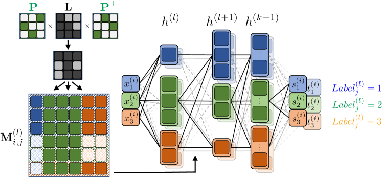
Figure 3: Network architecture of OCDaf with block masking matrices for a given ordering of $2<3<1$. Each color represents the neurons corresponding to one variable. In the final layer, self-connections are absent, and each neuron depends solely on inputs with smaller labels.

One distinction between OCDaf and other similar permutation learning causal discovery algorithms such as Charpentier et al. [25] is that we incorporate the permutation directly into our architecture. In contrast, other works generally apply permutations to model input. In the latter case, model weights acquire different meanings for each input configuration. In our architecture, however, the weight between covariates $i$ and $j$ consistently corresponds to their dependencies and is either masked or facilitated by a specific permutation. This allows for parameter sharing and increased utilization considering multiple permutations – A sufficiently large network can represent the optimal weights for all permutations.

Our experiments also consider an alternative approach to the Gumbel-Top-k trick and straight-through gradient estimator for permutation learning. Since for sufficiently low temperature $\tau$, the matching operator $M(\Gamma)$ is closely approximated by the Sinkhorn operator $S(\Gamma/\tau)$, we can directly use the soft samples from the Sinkhorn operator in the forward and backward passes as the permutation matrix $\mathbf{P}$. We call this approach ”Soft” Sinkhorn. However, since the whole optimization procedure is end-to-end, the model is inclined to modify the value of $\Gamma$ such that its scale cancels the effect of small $\tau$, a necessary condition for the Sinkhorn operator to generate precise permutation matrices. As a result, the matrices generated by the Sinkhorn operator evolve into soft doubly stochastic matrices, which can potentially introduce loops into the covariate dependency graphs. These loops significantly influence the training process and can result in a misleading value of the proxy loss. We empirically illustrate this phenomenon in Table 3.

Table 3: A comparison between OCDaf and the Soft Sinkhorn method across our small synthetic datasets. Although a lower proxy loss is preferable, Soft Sinkhorn yields misleading low loss values while generating near-random orderings as captured by CBC, implying self-loops.

Method	Avg. CBC	Avg. Proxy Loss
Soft Sinkhorn	0.49	-8.77
OCDaf (Top-k)	0.14	2.38
OCDaf (Sinkhorn)	0.35	2.53

Appendix F The Synthetic Benchmark

We devised a comprehensive benchmark suite to facilitate a robust evaluation of our proposed method. This benchmark provides a flexible and reproducible means of generating diverse datasets based on various graph structures and functional forms. We partitioned the Structural Causal Model (SCM) generation process into four distinct phases:

• Graph Generation: Our benchmark generates random graphs of varying sizes. We classify these graphs into three types:

  • Causal Paths: These causal graphs follow a strict sequence of cause and effect. These graphs are sparse and have unique correct orderings.

  • Full Graphs (Tournaments): These causal graphs also possess a unique ordering, where the $i$th variable depends on all preceding variables.

  • Erdős–Rényi Random Graphs: Based on the graph generation method proposed by Erdős et al. [61]. These random graphs can have multiple correct orderings.

• Functional Form Generation: Following the graph generation phase, we now formulate the functional relationships between the parent-children variables. We consider LSNMs (Definition 3.2) as our data generating models:

  $$X_{i}=f_{i}(\mathbf{PA}_{i})+g_{i}(\mathbf{PA}_{i})\cdot U_{i}$$

  Our code is designed to generate datasets under the following regimes:

  • Linear: Here, both $f_{i}$ and $g_{i}$ are random linear combinations of the inputs. To mitigate var-sortability, we normalize the data while simulating the data-generating process along the correct graph ordering [57].

  • Sinusoidal Parametric: This parametric model is designed to generate GI-LSNM datasets satisfying the identifiability criterion specified in Definition 4.1. We apply the invertible $\sin(x)+x$ function to a linear combination of parents for each covariate to introduce non-linearity into $f_{i}$ and enforce positivity in $g_{i}$ using a softplus function.

  • Polynomial Parametric: Similar to the Sinusoidal parametric scheme, we introduce non-linearity into $f_{i}$ via a polynomial $x^{3}+b$ (where $b$ is randomly selected) and apply a softplus function to ensure $g_{i}$ remains positive. The data is normalized during generation to prevent exponential growth.

  • Non-parametric: Following Zhu et al. [56], we sample functions $f_{i}$ and $g_{i}$ from Gaussian processes. To ensure positivity, $g_{i}$ also passes through a softplus.

• Noise Generation: To emphasize the potential impacts of model misspecification, we consider both Gaussian and non-Gaussian (specifically, Laplace) noise distributions for our benchmarks.

• Affine/Additive Testing: We also include simulations where $g_{i}$ is a constant function, enabling a comparison with other baseline models that only work in additive settings.

In all our experiments, we take $1000$ samples from each of the specified SCMs is $1000$ with different random seeds for graph generation, function creation, and data simulation. A summary of all the datasets incorporated into our benchmark is shown in Table 4.

Table 4: Summary of the Synthetic Benchmark Datasets.

Affine or Additive	Functional Form	Graph Size	Graph Type	Noise	# of Simulations
Affine	Nonparametric	$3\leq d\leq 6$	Erdős–Rényi	Normal	20
Affine	Nonparametric	$3\leq d\leq 6$	Tournament	Normal	20
Affine	Nonparametric	$3\leq d\leq 6$	Path	Normal	20
Additive	Nonparametric	$3\leq d\leq 6$	Erdős–Rényi	Normal	20
Additive	Nonparametric	$3\leq d\leq 6$	Tournament	Normal	20
Additive	Nonparametric	$3\leq d\leq 6$	Path	Normal	20
Affine	Linear	$3\leq d\leq 6$	Erdős–Rényi	Laplace	20
Affine	Linear	$3\leq d\leq 6$	Tournament	Laplace	20
Affine	Linear	$3\leq d\leq 6$	Path	Laplace	20
Additive	Linear	$3\leq d\leq 6$	Erdős–Rényi	Laplace	20
Additive	Linear	$3\leq d\leq 6$	Tournament	Laplace	20
Additive	Linear	$3\leq d\leq 6$	Path	Laplace	20
Affine	Nonparametric	$d\in\{10,25\}$	Erdős–Rényi	Normal	10
Affine	Sinusoidal	$d\in\{10,25\}$	Erdős–Rényi	Normal	10
Affine	Polynomial	$d\in\{10,25\}$	Erdős–Rényi	Normal	10
Affine	Sinusoidal	$3\leq d\leq 6$	Erdős–Rényi	Normal	20
Affine	Sinusoidal	$3\leq d\leq 6$	Tournament	Normal	20
Affine	Sinusoidal	$3\leq d\leq 6$	Path	Normal	20
Affine	Polynomial	$3\leq d\leq 6$	Erdős–Rényi	Normal	20
Affine	Polynomial	$3\leq d\leq 6$	Tournament	Normal	20
Affine	Polynomial	$3\leq d\leq 6$	Path	Normal	20
Affine	Linear	$3\leq d\leq 6$	Erdős–Rényi	Normal	20
Affine	Linear	$3\leq d\leq 6$	Tournament	Normal	20
Affine	Linear	$3\leq d\leq 6$	Path	Normal	20
Additive	Sinusoidal	$3\leq d\leq 6$	Erdős–Rényi	Normal	20
Additive	Sinusoidal	$3\leq d\leq 6$	Tournament	Normal	20
Additive	Sinusoidal	$3\leq d\leq 6$	Path	Normal	20
Additive	Polynomial	$3\leq d\leq 6$	Erdős–Rényi	Normal	20
Additive	Polynomial	$3\leq d\leq 6$	Tournament	Normal	20
Additive	Polynomial	$3\leq d\leq 6$	Path	Normal	20
Additive	Linear	$3\leq d\leq 6$	Erdős–Rényi	Normal	20
Additive	Linear	$3\leq d\leq 6$	Tournament	Normal	20
Additive	Linear	$3\leq d\leq 6$	Path	Normal	20

The summarized results for small graph benchmarks are provided in Table 2. To evaluate the scalability of our model, we extend the analysis to large, random graphs with $d\in\{10,25\}$, as presented in Table 5. The results reveal that our model consistently outperforms others when handling data in parametric function forms. In non-parametric scenarios, it performs equally well as the top baselines for $d=10$ but shows less efficacy for $d=25$. We hypothesize that increasing the number of epochs could improve this performance. However, these findings also suggest certain limitations in our proposed model’s capabilities, especially when scaling.

Table 5: Comparison of baseline methods with OCDaf Gumbel-Top-k on large scale synthetic datasets in terms of CBC (presented as mean $\pm$ standard deviation across samples).

	Large Datasets
Method	Parametric		Non-parametric
	$d=10$	$d=25$	$d=10$	$d=25$
OCDaf (Top-k)	$\mathbf{0.16\pm 0.08}$	$\mathbf{0.24\pm 0.03}$	$\mathbf{0.2\pm 0.06}$	$0.54\pm 0.05$
CAM	$0.85\pm 0.12$	$0.9\pm 0.07$	$0.27\pm 0.23$	$0.28\pm 0.18$
VI-DP-DAG	$0.64\pm 0.22$	$0.59\pm 0.11$	$0.46\pm 0.23$	$0.44\pm 0.12$
DAGuerreo	$0.88\pm 0.07$	$0.88\pm 0.04$	$0.3\pm 0.07$	$0.38\pm 0.06$
SCORE	$0.9\pm 0.1$	$0.96\pm 0.03$	$\mathbf{0.2\pm 0.09}$	$\mathbf{0.17\pm 0.06}$
VarSort	$0.86\pm 0.08$	$0.84\pm 0.11$	$0.49\pm 0.11$	$0.55\pm 0.07$
biLSNM	$0.62\pm 0.09$	$0.52\pm 0.04$	$0.65\pm 0.12$	$0.54\pm 0.03$

Appendix G Experimental Details

Gumbel Noise Scheduling. OCDaf incorporates a strategy of annealing the Gumbel noises added to $\Gamma$. We utilize a large standard deviation for the Gumbel noise during the initial phase, ensuring a broad coverage of the permutation set $\mathcal{H}_{k}$. As training proceeds, we move to a smaller locality by ultimately reducing the Gumbel noise standard deviation to zero. This approach ensures that generated permutations are centered on the single point $M(\Gamma)$, leading to deterministic outcomes. For most of our experiments, we implement a linear annealing strategy for the noise standard deviation.

Data Standardization. To enhance model stability, we standardize the data before feeding it to the model. Furthermore, we utilize an outlier detection scheme, removing $x(v)$ values that deviate significantly from the $x(v)$ median. Note that scaled and shifted datasets generated by LSNMs or ANMs remain within the same model class.

Numerical Stability. In our implementation, we feed $s_{i}^{\theta}(\mathbf{x}_{<\pi(i)})$ to an exponential function to guarantee positivity. The inherent numerical instability of this function can result in gradient explosion. To mitigate this, we adopt two techniques:

• Clipping all backpropagation gradients.

• Implementing a differentiable scaling and shifting function, using $\tanh$, before passing them through the exponential function. Specifically, denoting the output of previous layers as $u$, we compute $s_{i}^{\theta}=\tanh(u/a)\times b$. This ensures that the value lies in the range $[-b,+b]$ with the scaling factor $a$ maintaining sufficiently scaled gradients to prevent them from vanishing.

Regularization. We apply an element-wise Sigmoid function on the permutation parameter $\Gamma$ to avoid extreme values. We also employ the Adam optimizer with weight decay.

Phase-Changing Training Scheme. Our approach employs a two-phase training methodology, alternating between training $\theta$ and $\Gamma$. This technique yields superior results in practice and aligns with our theoretical understanding of the training process. The first phase, referred to as ”maximization,” focuses on training $\theta$. During this phase, the model strives to learn $\ell_{N}(\mathbf{P};\theta)$ for $\mathbf{P}\in\mathcal{H}_{k}$, encouraging the model to converge towards an ensemble capable of generating high likelihood values for permutations sourced from $\mathcal{H}_{k}$. The training transitions to the second phase after sufficient training of $\ell_{N}(\mathbf{P};\theta)$. During this phase, referred to as the ”expectation” phase, the learning process is concentrated on $\Gamma$, and the learned $\Gamma$ leads to permutation distributions with higher likelihoods. Note that moving into the second phase without adequately training $\ell_{N}(\mathbf{P};\theta)$ can result in error propagation. This can consequently cause the model to increasingly focus on an erroneous permutation, affecting the overall performance.

G.1 Visualization for the Gumbel Sinkhorn Method

Figure 4 provides an illustrative depiction of the distinct training stages of our proposed Gumbel-Sinkhorn method within the Birkhoff polytope. We perform a PCA on all permutation matrices during our training process. At each stage, we sample a set of Gumbel noises, denoted as $\epsilon_{1}\ldots\epsilon_{k}$. The color-coded dots shown represent the Sinkhorn operator’s output: $S\left(\frac{\Gamma+\epsilon_{i}}{\tau}\right)$, indicating that each sample, after the Sinkhorn operation, resides within the Birkhoff Polytope. Each color demonstrates the permutation matrix after applying the matching operator $M(\Gamma+\epsilon_{i})$. The cross in the figures shows the noise-free $\Gamma$ or $S\left(\frac{\Gamma}{\tau}\right)$, illustrating the model parameters’ location in the Birkhoff Polytope’s latent space. The vertices of the Birkhoff are color-coordinated based on their corresponding permutations CBC. As depicted, the model initiates from a specific point, incrementally progressing towards the accurate permutation with the minimum CBC.

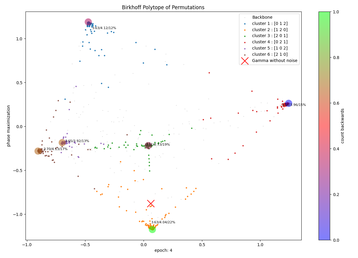
(a) Beginning.

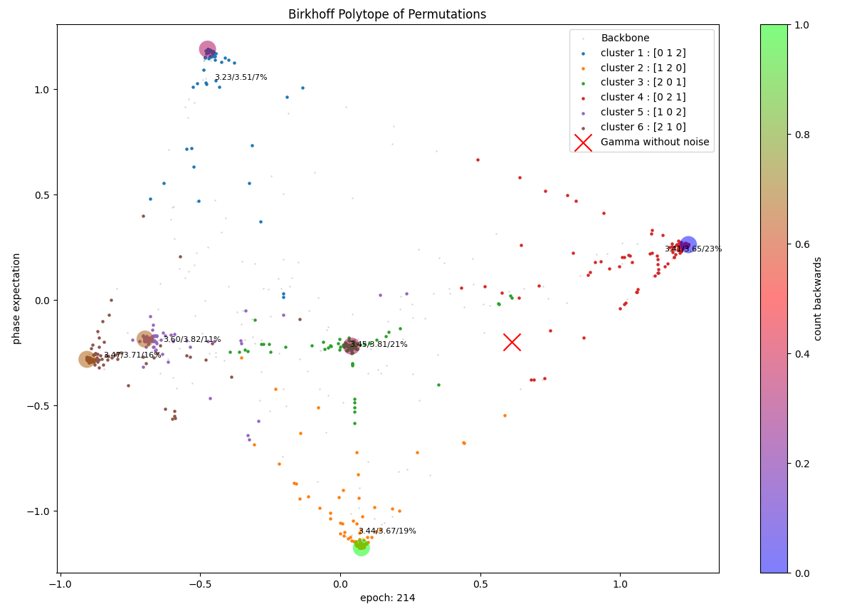
(b) Mid-training.

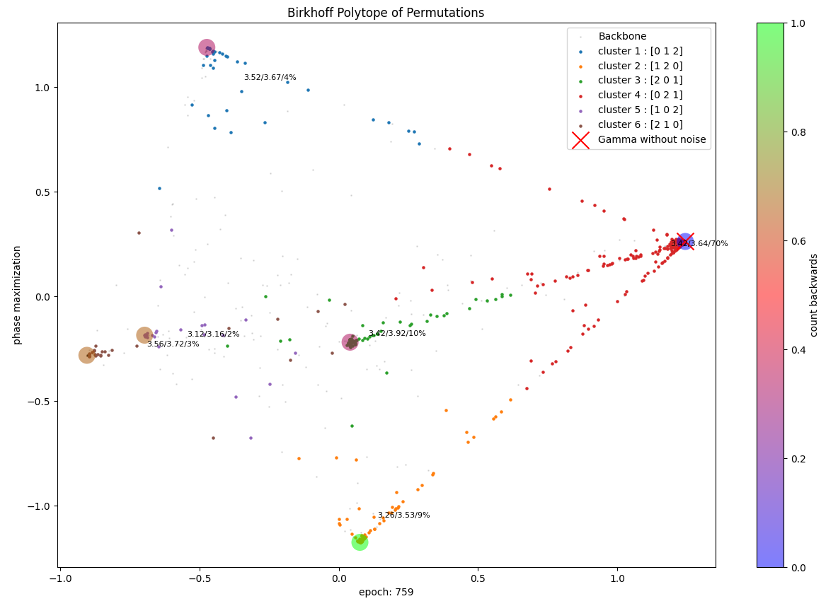
(c) Ending.

Figure 4: Training of the Gumbel-Sinkhorn method in the Birkhoff polytope.

G.2 Evaluation on Real-World and Semi-Synthetic Datasets

To compare our method fairly with other baselines, we utilized the Sachs and SynTReN datasets, benchmarking our results via standard metrics such as SHD and SID. Our approach starts by learning the true ordering and constructs a full tournament graph based on this ordering. To convert the resulting dense causal graph into a sparse one, we apply the following two pruning techniques:

• CAM pruning: Originating from Bühlmann et al. [15], CAM employs Lasso sparse regression for pruning. Even though it is originally designed for homoscedastic settings, we extend its application to the Sachs and Syntren datasets. This flexibility illustrates the method’s potential for use in diverse datasets.

• PC-KCI: This technique leverages conditional independence testing in Zhang et al. [59] to derive a valid causal graph skeleton. Once this skeleton is obtained, we integrate the learned ordering to retrieve the complete graph. This combination of steps ensures the production of a robust and reliable causal graph.

For the Sachs dataset, we run the algorithm using $5$ different seeds and report the metrics’ average and standard deviation. 1

G.3 Baselines

To ensure a comprehensive and fair comparison, all baselines are run with and without data standardization for the Sachs and Syntren datasets. The best model is selected based on the CBCmetric, providing an objective performance evaluation. We run some of the baselines with additional hyperparameter tuning:

• CAM: We consider both linear and nonlinear regression models.

• DAGuerreo: We test both SparseMAP and Top-k sparsemax options and linear and nonlinear equation models.

• VI-DP-DAG: This baseline is trained with both Gumbel-Top-k and Sinkhorn alternatives. We also consider a range of epochs, setting a maximum limit of 100 or 1000 to assess performance impact.

After testing, we employ all methods with their respective best-performing hyperparameters based on the CBCmetric on the Sachs dataset. Once the most effective hyperparameters are determined, we fix these settings for all synthetic data experiments.

Appendix H Interventional Distributions

To investigate the capability of our model in estimating downstream interventional distributions, we hand-craft experimental datasets that exhibit interesting trends in their interventional distributions. Our practical observations suggest that uncovering the right causal ordering may suffice for estimating interventions.

H.1 Setup

Dataset. Similar to the general LSNM datasets in the rest of the paper, we synthesize parametric distribution for a given causal ordering $\pi$ and exogenous noises $U$ as:

$$X_{i}=f(\mathbf{PA}_{\pi_{i}},U_{i})=s(\oplus_{s}^{\mathbf{w}}(\mathbf{PA}_{\pi_{i}}))U_{i}+t(\oplus^{\mathbf{w}}_{t}(\mathbf{PA}_{\pi_{i}}))$$

where $\mathbf{PA}_{\pi_{i}}$ denotes the parent nodes for $X_{i}$ in the ordering $\pi$ and $s,t:\mathcal{R}\to\mathbb{R}$ are functions for the scale and location in our LSNM. The $\oplus_{j}^{\mathbf{w}}$ denotes a linear combination of its inputs based on an arbitrary weighting vector $\mathbf{w}_{j}$.

To capture the various types of dependencies that occur when computing interventions, we examine two types of causal graphs: Tournaments and causal paths, as defined in Appendix F. Furthermore, we set $s$ to be of the form $\alpha-\beta e^{-\frac{|x|}{2}}$ ($\alpha>\beta$) so that the variance of the predictions increases as we move away from the center of the root node $x_{0}$. In our experiments, we set $\alpha=0.15$ and $\beta=0.12$. On the other hand, we examine two different function forms for $t$. The first form is $t(x)=x+\sin(x)$, which defines an identifiable LSNM model (used for Figure 2). The second one is $t(x)=\sin(\frac{2x}{3})+\sin(\frac{3x}{2})$, defining a model outside of the GI-LSNM assumptions. Finally, in all the datasets for the interventional experiments, we choose $P_{U}$ as a standard Gaussian distribution.

Training a Fixed Ordering Model. To explore the properties of interventional distribution estimation independently, we assume the true causal ordering $\pi$ is either known or has been identified by running OCDaf. Given $\pi$, we calculate the masks for our model and train it to minimize the negative-log-likelihood of observational samples generated from the aforementioned dataset.

Estimating Interventional Distributions. For ease of notation, we assume the correct causal ordering as ${1<2<\cdots<n}$. We are interested in samples from the hard interventional distribution $P(\mathbf{X}|do(X_{1})=y)$. Given a trained model $\mathbf{X}=T(\mathbf{}U)$, we can sample from the interventional distribution using the procedure described in Algorithm 2, a similar approach to Khemakhem et al. [8].

Input: The value of $y$ for $do(X_{1})=y$

Output: A single sample drawn from $P(\mathbf{X}|do(X_{1})=y)$

$U_{1}\leftarrow T_{1}^{-1}(y)$ # compute the associated $U_{1}$ which results in $X_{1}=y$

$U_{\{2,\cdots,n\}}\sim P_{U}$ # sample the rest of the noises

return $T(\mathbf{U})$ # a sample from the hard interventional distribution

Algorithm 2 Generating samples from the hard interventional distribution

To report the interventional distribution for a node of interest, we use $50$ independently drawn samples from that distribution to estimate the mean and the $99\%$ confidence interval.

H.2 Results

Tournaments. In this setting, which has been used to produce the results in Figure 2 and Figure 5, we employ a two-layered Masked MLP architecture with two layers of $5$ and $3$ neurons per node (hence $25$ and $15$ neurons in total) with Leaky ReLU activation functions to model $s$ and $t$ functions. We use a ReduceLROnPlateau scheduler on top of the AdamW optimizer to fit the synthetic dataset using $4000$ samples. We choose the flow’s base distribution as a standard Gaussian to match the exogenous noises in our data.

Figure 2 and Figure 5 report the estimated interventional expected values of the trained model. We observe that the trained model can accurately estimate the interventional distributions in the $99\%$ confidence interval of $X_{1}$.

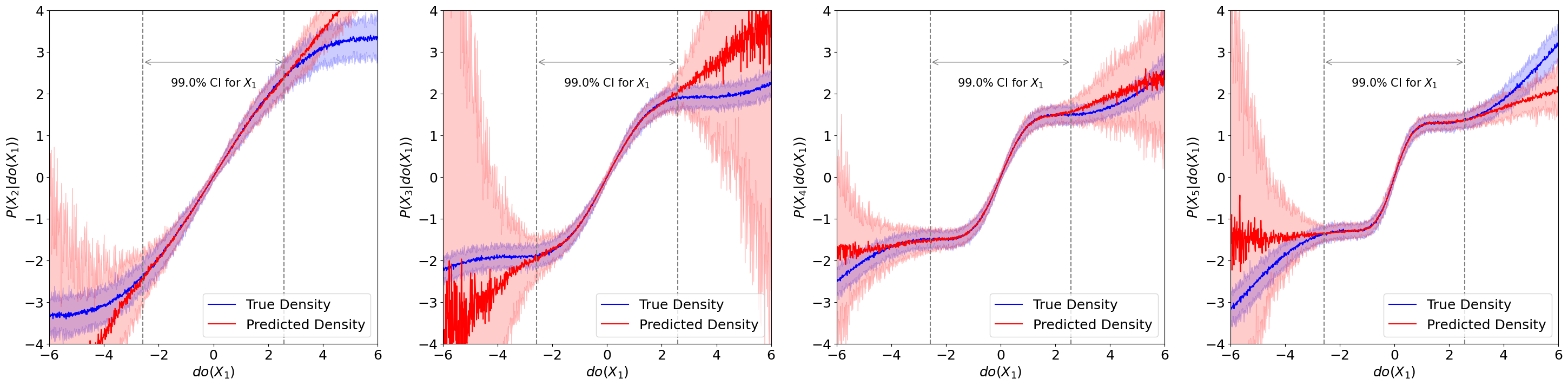
Figure 5: Estimation of intermediate interventional expected values in a causal tournament with $X_{1}$ and $X_{5}$ being the first and last nodes.

Causal Paths. Here, we train a larger network with three hidden layers of $30$, $20$, and $10$ neurons per node to fit $4000$ observational samples of a three-node causal path with $t(x)=\sin(\frac{2x}{3})+\sin(\frac{3x}{2})$. We leave the rest of the hyperparameters similar to those above. Figure 6 shows that a large enough model can accurately estimate the interventional expected values in regimes where the observational samples are concentrated. However, the predictions deviate significantly from the ground truth distributions outside of that regime.

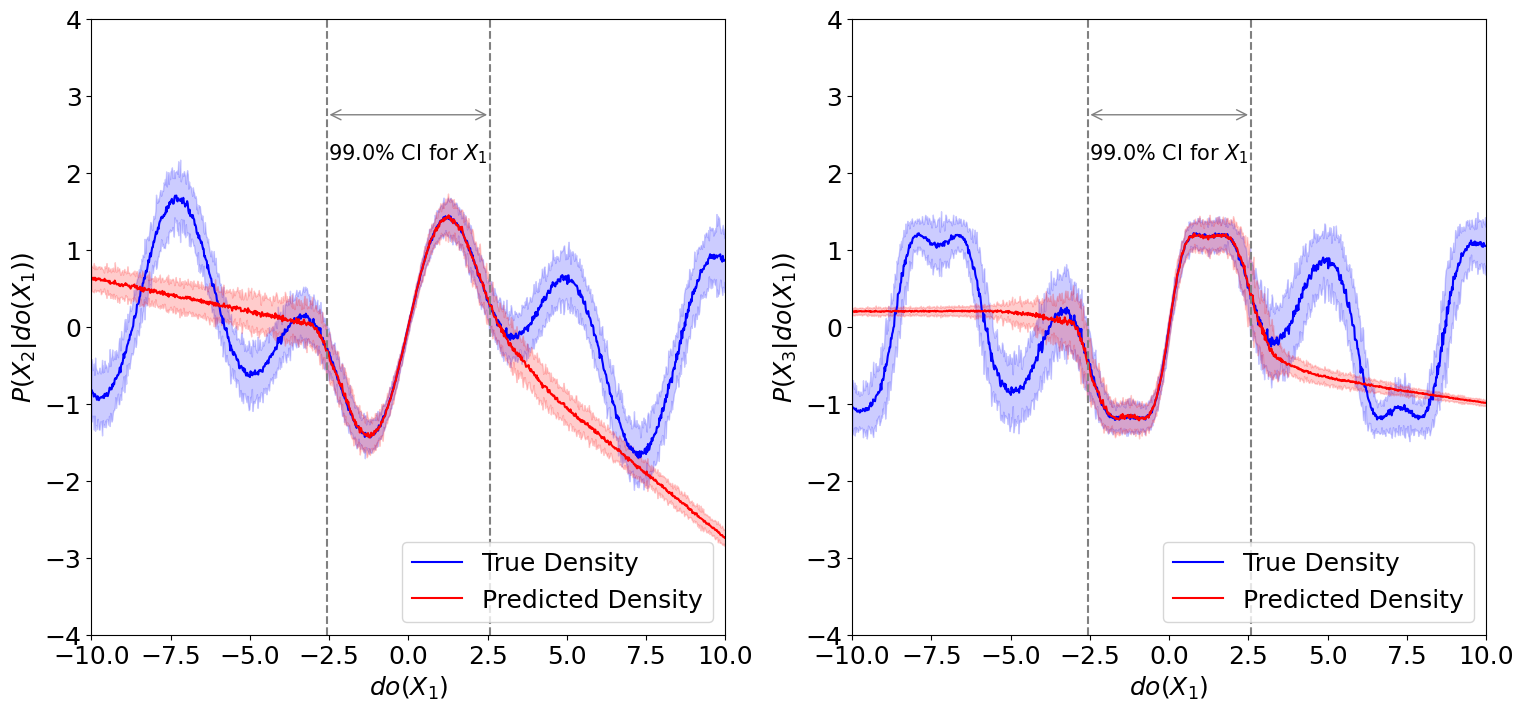
Figure 6: Estimation of intermediate interventional expected values in a causal path with $X_{1}$ and $X_{3}$ being the first and last nodes.

References

- Pearl [2009] Judea Pearl. Causality. Cambridge university press, 2009.
- Sachs et al. [2005] Karen Sachs, Omar Perez, Dana Pe’er, Douglas A Lauffenburger, and Garry P Nolan. Causal protein-signaling networks derived from multiparameter single-cell data. Science, 308(5721):523–529, 2005.
- Zhang et al. [2013] Bin Zhang, Chris Gaiteri, Liviu-Gabriel Bodea, Zhi Wang, Joshua McElwee, Alexei A Podtelezhnikov, Chunsheng Zhang, Tao Xie, Linh Tran, Radu Dobrin, et al. Integrated systems approach identifies genetic nodes and networks in late-onset alzheimer’s disease. Cell, 153(3):707–720, 2013.
- Peters et al. [2013] Jonas Peters, Joris Mooij, Dominik Janzing, and Bernhard Schölkopf. Causal discovery with continuous additive noise models. Journal of Machine Learning Research, 15, 09 2013. doi: 10.15496/publikation-1672.
- Imoto et al. [2003] Seiya Imoto, Sunyong Kim, Takao Goto, Sachiyo Aburatani, Kousuke Tashiro, Satoru Kuhara, and Satoru Miyano. Bayesian network and nonparametric heteroscedastic regression for nonlinear modeling of genetic network. Journal of bioinformatics and computational biology, 1(02):231–252, 2003.
- White [1980] Halbert White. A heteroskedasticity-consistent covariance matrix estimator and a direct test for heteroskedasticity. Econometrica: journal of the Econometric Society, pages 817–838, 1980.
- Engle [1982] Robert F Engle. Autoregressive conditional heteroscedasticity with estimates of the variance of united kingdom inflation. Econometrica: Journal of the econometric society, pages 987–1007, 1982.
- Khemakhem et al. [2021] Ilyes Khemakhem, Ricardo Monti, Robert Leech, and Aapo Hyvarinen. Causal autoregressive flows. In International conference on artificial intelligence and statistics, pages 3520–3528. PMLR, 2021.
- Solus et al. [2021] Liam Solus, Yuhao Wang, and Caroline Uhler. Consistency guarantees for greedy permutation-based causal inference algorithms. Biometrika, 108(4):795–814, 2021.
- Immer et al. [2022] Alexander Immer, Christoph Schultheiss, Julia E Vogt, Bernhard Schölkopf, Peter Bühlmann, and Alexander Marx. On the identifiability and estimation of causal location-scale noise models. arXiv preprint arXiv:2210.09054, 2022.
- Chickering et al. [2004] Max Chickering, David Heckerman, and Chris Meek. Large-sample learning of bayesian networks is np-hard. Journal of Machine Learning Research, 5:1287–1330, 2004.
- Spirtes et al. [2000] Peter Spirtes, Clark N Glymour, Richard Scheines, and David Heckerman. Causation, prediction, and search. MIT press, 2000.
- Zhang [2008] Jiji Zhang. On the completeness of orientation rules for causal discovery in the presence of latent confounders and selection bias. Artificial Intelligence, 172(16-17):1873–1896, 2008.
- Chickering [2002] David Maxwell Chickering. Optimal structure identification with greedy search. Journal of machine learning research, 3(Nov):507–554, 2002.
- Bühlmann et al. [2014] Peter Bühlmann, Jonas Peters, and Jan Ernest. Cam: Causal additive models, high-dimensional order search and penalized regression. The Annals of Statistics, 42(6):2526–2556, 2014.
- Bouckaert [1992] Remco R Bouckaert. Optimizing causal orderings for generating dags from data. In Uncertainty in Artificial Intelligence, pages 9–16. Elsevier, 1992.
- Singh and Valtorta [1993] Moninder Singh and Marco Valtorta. An algorithm for the construction of bayesian network structures from data. In Uncertainty in artificial intelligence, pages 259–265. Elsevier, 1993.
- Friedman and Koller [2003] Nir Friedman and Daphne Koller. Being bayesian about network structure. a bayesian approach to structure discovery in bayesian networks. Machine learning, 50(1):95–125, 2003.
- Scanagatta et al. [2015] Mauro Scanagatta, Cassio P de Campos, Giorgio Corani, and Marco Zaffalon. Learning bayesian networks with thousands of variables. Advances in neural information processing systems, 28, 2015.
- Park and Klabjan [2017] Young Woong Park and Diego Klabjan. Bayesian network learning via topological order. The Journal of Machine Learning Research, 18(1):3451–3482, 2017.
- Teyssier and Koller [2012] Marc Teyssier and Daphne Koller. Ordering-based search: A simple and effective algorithm for learning bayesian networks. arXiv preprint arXiv:1207.1429, 2012.
- Zheng et al. [2018] Xun Zheng, Bryon Aragam, Pradeep K Ravikumar, and Eric P Xing. Dags with no tears: Continuous optimization for structure learning. Advances in Neural Information Processing Systems, 31, 2018.
- Lachapelle et al. [2019] Sébastien Lachapelle, Philippe Brouillard, Tristan Deleu, and Simon Lacoste-Julien. Gradient-based neural dag learning. arXiv preprint arXiv:1906.02226, 2019.
- Zheng et al. [2020] Xun Zheng, Chen Dan, Bryon Aragam, Pradeep Ravikumar, and Eric Xing. Learning sparse nonparametric dags. In International Conference on Artificial Intelligence and Statistics, pages 3414–3425. PMLR, 2020.
- Charpentier et al. [2022] Bertrand Charpentier, Simon Kibler, and Stephan Günnemann. Differentiable dag sampling. arXiv preprint arXiv:2203.08509, 2022.
- Zantedeschi et al. [2023] Valentina Zantedeschi, Luca Franceschi, Jean Kaddour, Matt J Kusner, and Vlad Niculae. Dag learning on the permutahedron. arXiv preprint arXiv:2301.11898, 2023.
- Geffner et al. [2022] Tomas Geffner, Javier Antoran, Adam Foster, Wenbo Gong, Chao Ma, Emre Kiciman, Amit Sharma, Angus Lamb, Martin Kukla, Nick Pawlowski, et al. Deep end-to-end causal inference. arXiv preprint arXiv:2202.02195, 2022.
- Kingma et al. [2016] Durk P Kingma, Tim Salimans, Rafal Jozefowicz, Xi Chen, Ilya Sutskever, and Max Welling. Improved variational inference with inverse autoregressive flow. Advances in neural information processing systems, 29, 2016.
- Kobyzev et al. [2020] Ivan Kobyzev, Simon JD Prince, and Marcus A Brubaker. Normalizing flows: An introduction and review of current methods. IEEE transactions on pattern analysis and machine intelligence, 43(11):3964–3979, 2020.
- Mena et al. [2018] Gonzalo Mena, David Belanger, Scott Linderman, and Jasper Snoek. Learning latent permutations with gumbel-sinkhorn networks. arXiv preprint arXiv:1802.08665, 2018.
- Kool et al. [2019] Wouter Kool, Herke Van Hoof, and Max Welling. Stochastic beams and where to find them: The gumbel-top-k trick for sampling sequences without replacement. In International Conference on Machine Learning, pages 3499–3508. PMLR, 2019.
- Van den Bulcke et al. [2006] Tim Van den Bulcke, Koenraad Van Leemput, Bart Naudts, Piet van Remortel, Hongwu Ma, Alain Verschoren, Bart De Moor, and Kathleen Marchal. Syntren: a generator of synthetic gene expression data for design and analysis of structure learning algorithms. BMC bioinformatics, 7:1–12, 2006.
- Vowels et al. [2022] Matthew J Vowels, Necati Cihan Camgoz, and Richard Bowden. D’ya like dags? a survey on structure learning and causal discovery. ACM Computing Surveys, 55(4):1–36, 2022.
- Chicharro et al. [2019] Daniel Chicharro, Stefano Panzeri, and Ilya Shpitser. Conditionally-additive-noise models for structure learning. arXiv preprint arXiv:1905.08360, 2019.
- Shimizu et al. [2006] Shohei Shimizu, Patrik O Hoyer, Aapo Hyvärinen, Antti Kerminen, and Michael Jordan. A linear non-gaussian acyclic model for causal discovery. Journal of Machine Learning Research, 7(10), 2006.
- Peters and Bühlmann [2014] Jonas Peters and Peter Bühlmann. Identifiability of gaussian structural equation models with equal error variances. Biometrika, 101(1):219–228, 2014.
- Chen et al. [2019] Wenyu Chen, Mathias Drton, and Y Samuel Wang. On causal discovery with an equal-variance assumption. Biometrika, 106(4):973–980, 2019.
- Gao et al. [2020] Ming Gao, Yi Ding, and Bryon Aragam. A polynomial-time algorithm for learning nonparametric causal graphs. Advances in Neural Information Processing Systems, 33:11599–11611, 2020.
- Gao and Aragam [2021] Ming Gao and Bryon Aragam. Efficient bayesian network structure learning via local markov boundary search. Advances in Neural Information Processing Systems, 34:4301–4313, 2021.
- Ghoshal and Honorio [2018] Asish Ghoshal and Jean Honorio. Learning linear structural equation models in polynomial time and sample complexity. In International Conference on Artificial Intelligence and Statistics, pages 1466–1475. PMLR, 2018.
- Monti et al. [2020] Ricardo Pio Monti, Kun Zhang, and Aapo Hyvärinen. Causal discovery with general non-linear relationships using non-linear ica. In Uncertainty in artificial intelligence, pages 186–195. PMLR, 2020.
- Strobl and Lasko [2022] Eric V Strobl and Thomas A Lasko. Identifying patient-specific root causes with the heteroscedastic noise model. arXiv preprint arXiv:2205.13085, 2022.
- Verma and Pearl [1990] Thomas Verma and Judea Pearl. Causal networks: Semantics and expressiveness. In Machine intelligence and pattern recognition, volume 9, pages 69–76. Elsevier, 1990.
- Ruiz et al. [2022] Gabriel Ruiz, Oscar Hernan Madrid Padilla, and Qing Zhou. Sequentially learning the topological ordering of causal directed acyclic graphs with likelihood ratio scores. arXiv preprint arXiv:2202.01748, 2022.
- Raskutti and Uhler [2018] Garvesh Raskutti and Caroline Uhler. Learning directed acyclic graph models based on sparsest permutations. Stat, 7(1):e183, 2018.
- Lam et al. [2022] Wai-Yin Lam, Bryan Andrews, and Joseph Ramsey. Greedy relaxations of the sparsest permutation algorithm. In Uncertainty in Artificial Intelligence, pages 1052–1062. PMLR, 2022.
- Wang et al. [2021] Xiaoqiang Wang, Yali Du, Shengyu Zhu, Liangjun Ke, Zhitang Chen, Jianye Hao, and Jun Wang. Ordering-based causal discovery with reinforcement learning. arXiv preprint arXiv:2105.06631, 2021.
- Rolland et al. [2022] Paul Rolland, Volkan Cevher, Matthäus Kleindessner, Chris Russell, Dominik Janzing, Bernhard Schölkopf, and Francesco Locatello. Score matching enables causal discovery of nonlinear additive noise models. In International Conference on Machine Learning, pages 18741–18753. PMLR, 2022.
- Sanchez et al. [2022] Pedro Sanchez, Xiao Liu, Alison Q O’Neil, and Sotirios A Tsaftaris. Diffusion models for causal discovery via topological ordering. arXiv preprint arXiv:2210.06201, 2022.
- Cundy et al. [2021] Chris Cundy, Aditya Grover, and Stefano Ermon. Bcd nets: Scalable variational approaches for bayesian causal discovery. Advances in Neural Information Processing Systems, 34:7095–7110, 2021.
- Bengio et al. [2013] Yoshua Bengio, Nicholas Léonard, and Aaron Courville. Estimating or propagating gradients through stochastic neurons for conditional computation. arXiv preprint arXiv:1308.3432, 2013.
- Niculae et al. [2018] Vlad Niculae, Andre Martins, Mathieu Blondel, and Claire Cardie. Sparsemap: Differentiable sparse structured inference. In International Conference on Machine Learning, pages 3799–3808. PMLR, 2018.
- Hazan et al. [2013] Tamir Hazan, Subhransu Maji, and Tommi Jaakkola. On sampling from the gibbs distribution with random maximum a-posteriori perturbations. Advances in Neural Information Processing Systems, 26, 2013.
- Tomczak [2016] Jakub M Tomczak. On some properties of the low-dimensional gumbel perturbations in the perturb-and-map model. Statistics & Probability Letters, 115:8–15, 2016.
- Papamakarios et al. [2017] George Papamakarios, Theo Pavlakou, and Iain Murray. Masked autoregressive flow for density estimation. Advances in neural information processing systems, 30, 2017.
- Zhu et al. [2019] Shengyu Zhu, Ignavier Ng, and Zhitang Chen. Causal discovery with reinforcement learning. arXiv preprint arXiv:1906.04477, 2019.
- Reisach et al. [2021] Alexander G Reisach, Christof Seiler, and Sebastian Weichwald. Beware of the simulated dag! varsortability in additive noise models. arXiv preprint arXiv:2102.13647, 2021.
- Peters and Bühlmann [2015] Jonas Peters and Peter Bühlmann. Structural intervention distance for evaluating causal graphs. Neural computation, 27(3):771–799, 2015.
- Zhang et al. [2012] Kun Zhang, Jonas Peters, Dominik Janzing, and Bernhard Schölkopf. Kernel-based conditional independence test and application in causal discovery. arXiv preprint arXiv:1202.3775, 2012.
- Germain et al. [2015] Mathieu Germain, Karol Gregor, Iain Murray, and Hugo Larochelle. Made: Masked autoencoder for distribution estimation. In International conference on machine learning, pages 881–889. PMLR, 2015.
- Erdős et al. [1960] Paul Erdős, Alfréd Rényi, et al. On the evolution of random graphs. Publ. Math. Inst. Hung. Acad. Sci, 5(1):17–60, 1960.