Tunneling probability for the birth of an universe with radiation in Hořava-Lifshitz theory
Abstract
In the present work, we study the birth of a homogeneous and isotropic Friedmann–Lemaître–Robertson–Walker (FLRW) cosmological model, considering Hořava-Lifshitz (HL) as the gravitational theory. The matter content of the model is a radiation perfect fluid. In order to study the birth of the universe in the present model, we consider the quantum cosmology mechanism of creation from nothing. In that mechanism, the universe appears after the wavefunction associated to that universe tunnels through a potential barrier. We started studying the classical model. We draw the phase portrait of the model and identify qualitatively all types of dynamical behaviors associated to it. Then, we write the Hamiltonian of the model and apply the Dirac’s quantization procedure to quantize a constrained theory. We find the appropriate Wheeler-DeWitt equation and solve it using the Wentzel–Kramers–Brillouin (WKB) approximation. Using the WKB solution, to the Wheeler-DeWitt equation, we compute the tunneling probabilities for the birth of that universe (). Since the WKB wavefunction depends on the radiation energy () and the free parameters coming from the HL theory (, , , ), we compute the behavior of as a function of and all the HL’s parameters , , , .
Keywords: Quantum cosmology, Hořava-Lifshitz theory, Radiation, Creation from nothing
PACS: 04.20.Dw, 04.50.Kd, 04.60.Ds , 98.80.Bp, 98.80.Qc
1 Introduction
Some years ago Petr Hořava introduced a new geometrical theory of gravity [1]. His main motivation was to obtain a renormalizable and unitary theory of gravity. One important ingredient of that theory, nowadays known as Hořava-Lifshitz theory, is an anisotropic scaling between space and time. That anisotropy is given by a critical exponent . Whenever that anisotropy or asymmetry between space and time is important the Lorentz symmetry is broken. It happens at high energies. At low energies HL theory tends to General Relativity (GR), which implies , and the Lorentz symmetry is recovered. In his original paper, Hořava formulated his theory using some elements of the Arnowitt-Deser-Misner (ADM) formalism [2]. In that formalism the four dimensional spacetime metric () is decomposed in terms of three dimensional metrics of spacelike sections (), the shift vector () and the lapse function (). In the most general situation all these quantities should depend on space and time. In order to facilitate the work with his theory, Hořava considered two simplifications. In the first one, he imposed that should depend only on the time variable [1]. This assumption is known as the projectable condition. In the second one, he reduced the number of terms contributing to the potential component of his theory [1]. It is known as the detailed balance condition. Unfortunately, it was shown that the projectable version of the HL theory, with the detailed balance condition, have massive ghosts and instabilities [3, 4]. Since its introduction many physicists have investigated different aspects of HL theory. In particular, when applied to cosmology it produced very interesting results [5, 6, 7, 8, 9, 10, 11, 12, 13, 14, 15, 16, 17, 18, 19, 20, 21, 22, 23, 24, 25, 26, 27, 28]. Some important aspects of the HL theory are discussed in Ref.[29].
The main motivation in order to quantize GR was the removal of physical singularities present in many cosmological as well as astrophysical solutions to Einstein’s equations. The first systematic approach toward the quantization of that theory was the canonical quantization. It started with the important works from P. A. M. Dirac on the correct Hamiltonian formulation of GR [30, 31, 32, 33]. After that, ADM gave an influential geometrical interpretation of the Hamiltonian formulation of GR [2]. Next, the canonical quantization of GR was performed, following Dirac’s instructions in order to quantize a constrained theory [30, 34], which lead to the famous Wheeler-Dewitt equations [35, 36]. When one applies that formalism to cosmological models one obtains a theory called Quantum Cosmology (QC). For a detailed introduction to QC see [37, 38, 39, 40]. One of the main applications of QC is the description of the beginning of the Universe. GR tells us that our Universe started in a huge explosion called Big Bang, which created space, time and some of the matter present in our Universe. GR, also, tell us that the Big Bang is a spacetime singularity. It means that GR loses its predictive power in the spacetime location of that catastrophic event. One of the most important results of QC is to offer a possible solution to the singular beginning of our Universe. That solution coming from QC uses, as a fundamental ingredient, the quantum mechanical tunneling mechanism and is usually referred to as spontaneous creation of the Universe from nothing (SCUFN)[41, 42, 43, 44, 45, 46, 47, 48]. In the SCUFN the Universe is at the origin of time and space and confined by a potential barrier. Since the Universe is a quantum mechanical system it may tunnel through the potential barrier and emerge to the right of it with a finite size. That moment marks the beginning of the Universe. Since the Universe starts with a finite size, it is free from the Big Bang singularity. In the literature, there are some works using these ideas in order to describe the birth of the universe in different cosmological models [49, 50, 51, 52, 53, 54, 55].
In the present paper, we want to study the birth of the universe in a cosmological model where the gravitational sector is described by the HL theory. Therefore, we consider a homogeneous and isotropic FLRW spacetime, with positively curved spatial sections (). The matter content of the model is a radiation perfect fluid. With respect to the HL theory, we consider the projectable version of that theory without the detailed balance condition. We start by writing the total Hamiltonian of the gravitational sector of the model, with the aid of the ADM formalism. Then, we obtain the total Hamiltonian of the matter sector of the model, with the aid of the Schutz variational formalism [56, 57]. Adding both total Hamiltonians, we find the total Hamiltonian of the model. From that total Hamiltonian, we notice that the potential barrier may have two different shapes. In the first one, it has a single barrier shape. In the second one, it has a well followed by a barrier shape. Due to the fact that the first barrier shape is a particular case of the second one, we restrict our attention to study the birth of the universe only for the second barrier shape. In order to learn more about that particular model, we study the classical dynamics of the scale factor. First, using the total Hamiltonian of the model we draw a phase portrait of the model, which gives a qualitative idea on the possible scale factor behaviors. Then, using once more the total Hamiltonian of the model we find and solve the Hamilton’s equations. We quantitatively obtain all possible scale factor solutions for the model. After that, we quantize the model following the Dirac’s formalism for constrained theories [30, 34], which produces the Wheeler-DeWitt equation of the model. We solve that equation using the WKB approximation and compute the appropriate tunneling probabilities for the birth of the universe (). Since is a function of the radiation fluid energy () and all the parameters coming from the HL theory (, , , ), we investigate, separately, how it depends on all these quantities.
In Section 2, we derive the total Hamiltonian, draw a phase portrait and solve the Hamilton’s equations for a homogeneous and isotropic HL cosmological model, with constant positive spatial sections and coupled to a radiation perfect fluid. In Section 3, we quantize the model and solve the resulting Wheeler-DeWitt equation, using the WKB approximation. In Section 4, we compute the WKB tunneling probabilities for the universe to tunnel through the potential barrier. We investigate how depends on , , , and . Finally, in Section 5, we summarize the main points and results of the paper. In Appendix A, we compute in details, with the aid of the Schutz variational formalism, the total Hamiltonian for the radiation fluid.
2 The Classical Model
We start by considering an isotropic and homogeneous Universe described by the FLRW metric,
| (1) |
where is called the lapse function and provides the curvature of the spacelike sections. may take the values , which gives, respectively, open, flat, or closed geometries. In the present work, we consider that the constant curvatures of the spacelike sections are positive (). We use the natural unit system where: . The matter content of the model is given by a radiation perfect fluid having a four-velocity given by: , in the co-moving coordinate system. The energy-momentum tensor is written as,
| (2) |
where and are the pressure and energy density of the fluid, respectively, and the Greek indexes and run from zero to three. Furthermore, the equation of state for the radiation perfect fluid is,
| (3) |
Selecting the projectable version of HL theory in the absence of the detailed balance condition, for in -dimensions, the action is given by,
| (4) |
where the ’s () and are parameters linked to HL theory, is the Planck mass, are the components of the extrinsic curvature tensor which has its trace denoted by . Also, are the components of the Ricci tensor computed for the metric of the three dimensional spatial sections, namely , and represents the covariant derivative in the direction. The Latin indices , and run from one to three. It is also important to comment that General Relativity is retrieved once one takes the limit .
Introducing the metric of the spatial sections that comes from the FLRW spacetime Eq. (1) in the action Eq. (4) and adopting the following values: and , we manage to write,
| (5) |
Here, one has that,
| (6) |
As a matter of simplicity let us consider . Using this condition, Eq. (5) may be written as,
| (7) |
where,
| (8) |
| (9) |
| (10) |
| (11) |
The equations running from (8-11) provide us with , and , the new coupling constants. It is important to mention that must be greater than zero (), because it is associated to the curvature coupling constant. The others may take positive or negative values. One may recall that so, for this action, one gets,
| (12) |
This allows us to compute the canonical momentum
| (13) |
Introducing the momentum Eq. (13) and the Lagrangian Eq. (12) into the total Hamiltonian definition and fixing , as mentioned above, one obtains,
| (14) |
which is the total Hamiltonian for the HL sector. The total Hamiltonian for the matter sector (), described by a radiation perfect fluid, is obtained through the Schutz Formalism. In Appendix A, we compute in details , whose expression is given by Eq. (46). Adding it to the HL total Hamiltonian (14), one finds,
| (15) |
In order to learn more about the scale factor classical behavior one should find and solve the Hamilton’s equations. These equations are computed with the aid of Eq. (15) and they are,
| (16) |
where the gauge was used and the dot means derivative with respect to the conformal time . If one imposes the constraint equation , and rewrite the resulting equation in terms of , with the aid of the first Hamilton’s equation Eq. (16), one finds,
| (17) |
where the classical potential is given by,
| (18) |
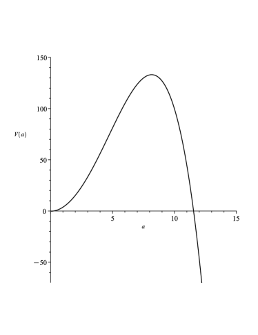
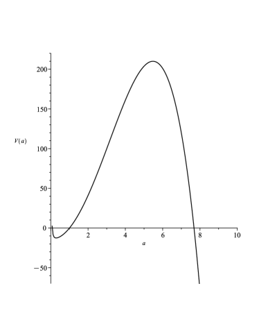
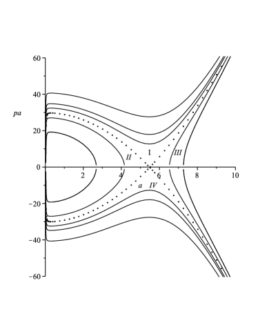
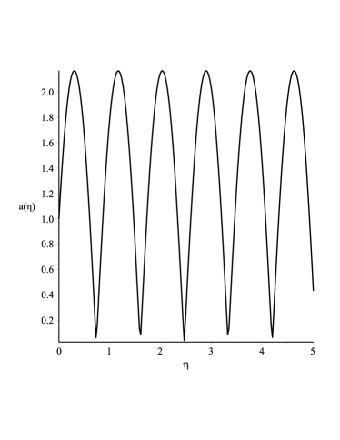
As mentioned above . is also positive because it is associated to the fluid energy density. In order to obtain well defined barrier type potentials, we study, here, models in which , and . For the choice , the potential develops an infinity positive barrier at the origin and those models are free from the big bang singularity. Taking in account those choices in the values of the HL’s parameters, we notice that Eq. (18) may have two different shapes depending on the values of these parameters. The first one has a single barrier and the second one has a well followed by a barrier. Examples for each potential shape are shown in Figures (1(a)) and (1(b)), respectively. The potential shown in Figure (1(a)) has a global maximum of while the one presented in Figure (1(b)) has a global maximum of and a local minimum of . Since the first type of potential (barrier) is much simpler and may be considered as a particular case of the second one (well followed by a barrier), in the present paper, we restrict our attention to study the second type of potential. In order to learn more about the present model, we study the classical dynamics of the scale factor. We start our study by drawing a phase portrait of the model. Figure (2) shows a phase portrait of the well followed by a barrier type of potential. There, the values of the HL’s parameters are the same ones used in Figure (1(b)).
After combining some of the Hamilton’s equations (16), we obtain the following second-order differential equation for the scale factor,
| (19) |
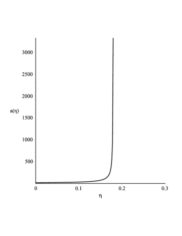
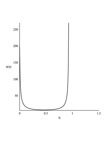
Solving Eq. (19) using the appropriate initial conditions, we find four different types of classical solutions for Eq. (18), when it has the shape of a well followed by a barrier Figure 1(b). The four types of solutions may be identified from the phase portrait Figure 2. They are: (i) An expansive solution where the scale factor starts expanding from a small value and continue expanding, in an accelerated rate, to infinity. This type of solution appears in region I of Figure 2. An example is given in Figure 3(a); (ii) A periodic solution where the scale factor starts expanding from a small value, reaches a maximum and then contracts back to the initial small value. This type of solution appears in region II of Figure 2. An example is given in Figure 3(b); (iii) A bouncing solution where the scale factor starts contracting from a large value, reaches a minimum value and then expands, in an accelerated rate, to infinity. This type of solution appears in region III of Figure 2. An example is given in Figure 4(a); (iv) A solution where the scale factor starts contracting from a large value and continue contracting to a small value. This type of solution appears in region IV of Figure 2. An example is given in Figure 4(b).

3 Canonical Quantization
In the present section, we want to quantize the model according to Dirac’s formalism for quantization of constrained systems. It starts by replacing the canonical variables and and theirs conjugated momenta by operators. Then, one must introduce the wavefunction of the Universe which is a function of the operators associated to the canonical variables, . The canonically conjugated momenta to and , respectively and , have the following operators expressions,
| (20) |
Next, one must impose the constraint equation,
| (21) |
where is obtained by replacing the operators expressions of , , and in the total Hamiltonian Eq. (15). The constraint equation (21), gives rise to the so-called Wheeler-DeWitt equation. Using the total Hamiltonian Eq. (15), the operators expressions of and Eq. (20), the gauge and the transformation , one obtains,
| (22) |
Presuming that one may write the solution to equation (22) as , after some calculations, one finds,
| (23) |
where is given by,
| (24) |
Now, suppose that the WKB approximation is valid for the present model [58, 59]. Once obtained, the WKB solution will be applied to compute the tunneling probabilities through the potential barrier . Following the WKB approximation, we write in Eq. (23) as . Introducing this ansatz in Eq. (23) and considering that is insignificant compared to the other terms in the resulting equation, we may write the following solution to that equation,
| (25) |
where,
| (26) |
is the value of where the energy intercepts, at the left, the potential (24), is the value of where the energy intercept, at the right, the potential (24) and , , , , and are constants.
Using matrix notation, one can relate A and B to F and G by,
| (27) |
where one has the parameter , which gives the barrier height and length, given by,
| (28) |
Now that the WKB solution was obtained, one has to compute the transmission coefficient, or tunneling probability, denoted by , through the potential barrier. If one considers that there is no wave coming from the right (),
| (29) |
From equation (27), one has,
| (30) |
Therefore, becomes,
| (31) |
For the present model, Eq. (28) is given, with the aid of Eq. (24) and Eq. (26), by,
| (32) |
4 Results
In the present section, we compute the Eq. (31), for the potential Eq. (24) which has the shape of a well followed by a barrier. As discussed earlier, we consider the models where , , and . In general, is a function of and the HL parameters. In order to establish how depends on those quantities, we fix all of them except the one we want to investigate. We repeat that procedure for many different values of all the quantities. In particular, when we study the dependence of with the HL parameters, we fix the same energy value for all parameters. Another important quantities, we must determine in order to compute are the scale factor values where the energy intercepts the potential at the left () and at the right (). In the following Subsections, we start that study.
4.1
In order to study how depends on the HL parameter , we fix appropriate values of , , and varies . We are considering only positive values of , because they produce an accelerate expansion of the universe. We repeat that procedure for a great number of appropriate values of all those quantities and reach the following conclusion: increases if one increases . Therefore, it is more likely that the universe is born with the greatest possible value of that parameter. We show an example of that result for a model where , , and . In the present example, we choose different values of : we start with all the way up to in steps of . For all chosen values of , the maxima values of the potentials Eq. (24) are greater than . In Figure 5, one can see the curve .
4.2
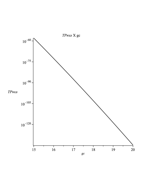
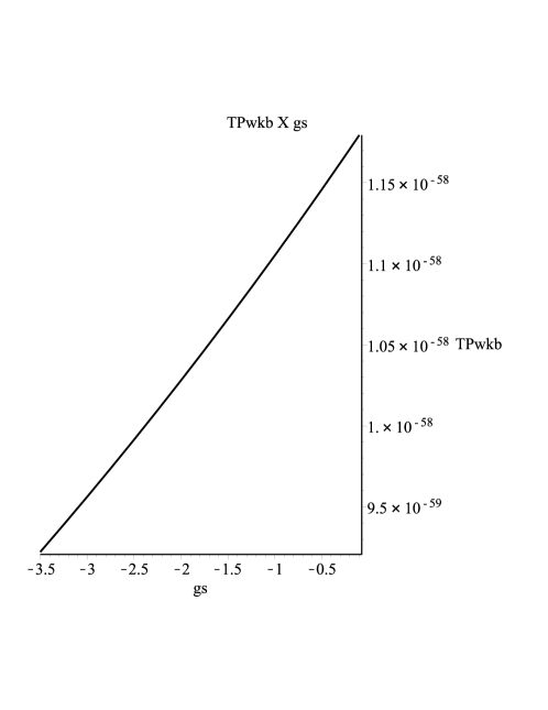
In order to study how depends on the HL parameter , we fix appropriate values of , , and varies . As we mentioned above, we are considering only positive values of . We repeat that procedure for a great number of appropriate values of all those quantities and reach the following conclusion: decreases if one increases . Therefore, it is more likely that the universe is born with the smallest possible value of that parameter. We show an example of that result for a model where , , and . In the present example, we choose different values of : we start with all the way up to in steps of . For all chosen values of , the maxima values of the potentials Eq. (24) are greater than . In Figure 6, one can see the curve .
4.3
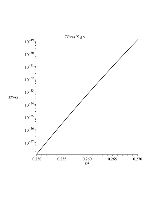
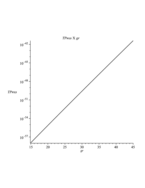
In order to study how depends on the HL parameter , we fix appropriate values of , , and varies . As we mentioned above, we are considering only negative values of . We repeat that procedure for a great number of appropriate values of all those quantities and reach the following conclusion: increases if one increases . Therefore, it is more likely that the universe is born with the greatest possible value of that parameter. We show an example of that result for a model where , , and . In the present example, we choose different values of : we start with , next and then it goes all the way down to in steps of . For all chosen values of , the maxima values of the potentials Eq. (24) are greater than . In Figure 7, one can see the curve .
4.4
In order to study how depends on the HL parameter , we fix appropriate values of , , and varies . We are considering only positive values of , because we want that the potential well has a negative minimum value. We repeat that procedure for a great number of appropriate values of all those quantities and reach the following conclusion: increases if one increases . Therefore, it is more likely that the universe is born with the greatest possible value of that parameter. We show an example of that result for a model where , , and . In the present example, we choose different values of : we start with all the way up to in steps of . For all chosen values of , the maxima values of the potentials Eq. (24) are greater than . In Figure 8, one can see the curve .
4.5
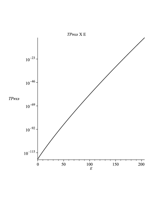
In order to study how depends on the radiation fluid energy , we fix appropriate values of , , and varies . We are considering only positive values of . We repeat that procedure for a great number of appropriate values of all those quantities and reach the following conclusion: increases if one increases . Therefore, it is more likely that the universe is born with the greatest possible value of the radiation fluid energy. We show an example of that result for a model where , , and . In the present example, we choose different values of : we start with all the way up to in steps of different sizes. For all chosen values of , the maximum value of the potential Eq. (24) is greater than E. In Figure 9, one can see the curve .
5 Conclusions
In the present paper, we investigated the birth of the universe in a cosmological model constructed using HL theory. We considered a homogeneous and isotropic FRW spacetime, with positively curved spatial sections (). The matter content of the model is a radiation perfect fluid. We restricted our attention to the projectable version of HL theory, without the detailed balance condition. Initially, we wrote the total Hamiltonian of the gravitational sector of the model, with the aid of the ADM formalism. Then, we obtained the total Hamiltonian of the matter sector of the model, with the aid of the Schutz variational formalism [56, 57]. Adding both total Hamiltonians, we found the total Hamiltonian of the model. From that total Hamiltonian, we noticed that the potential barrier could have two different shapes. In the first one, it has a single barrier shape. In the second one, it has a well followed by a barrier shape. Due to the fact that the first barrier shape is a particular case of the second one, we restricted our attention to the investigation of the birth of the universe only for the second barrier shape. In order to learn more about that particular model, we studied the classical dynamics of the scale factor. First, using the total Hamiltonian of the model we drew a phase portrait of the model, which gave a qualitative idea on the scale factor behavior. Then, using once more the total Hamiltonian of the model we found and solved the Hamilton’s equations. We quantitatively obtained all possible scale factor solutions for the model. After that, we quantized the model following Dirac’s formalism for constrained theories [30, 34], which produced the Wheeler-DeWitt equation. We solved that equation using the WKB approximation and computed the appropriate tunneling probabilities for the birth of the universe (). Since is a function of the radiation energy and all the parameters coming from the HL theory, we investigated, separately, how it depends on all these quantities. As the result of those investigations, we determined that: increases as , , and increase; and it decreases as increases. Therefore, it is more likely that the universe is born with the greatest possible values of , , and and with the smallest possible value of .
Acknowledgments. A. Oliveira Castro Júnior thanks Coordenação de
Aperfeiçoamento de Pessoal de Nível Superior (CAPES).
G. A. Monerat thanks FAPERJ for financial support and Universidade do Estado do Rio de Janeiro (UERJ) for the Prociência grant.
Appendix A Radiation fluid total Hamiltonian
In the Schutz variational formalism, for FRW cosmological models, the fluid four-velocity is given in terms of the following thermodynamical potentials , and ,
| (33) |
where is the specific enthalpy, is the specific entropy and the potentials and have no clear physical meaning. The four-velocity must satisfy the following normalization condition,
| (34) |
In order to obtain the final result, we must consider few equations coming from thermodynamics,
| (35) |
where is the specific internal energy, is the absolute temperature and is the rest mass density. From the combination of equations (35), it is possible to write,
| (36) |
Next, one may express in terms of the thermodynamical potentials , and Eq.(33). In order to do that, one must use Eq.(34),
| (37) |
In the next step, we want to write the radiation energy density as a function of , and . We do that with the aid of Eqs. (35), (36) and (37),
| (38) |
Now, we must introduce Eq.(38) in the perfect fluid action, which is given by,
| (39) |
where is the determinant of the metric and is the fluid pressure. After doing that, we find with the aid of Eq.(3) the following expression for the radiation fluid action,
| (40) |
It is straightforward to find the fluid Lagrangian from the action Eq.(40), which is given by,
| (41) |
Using the usual definition, we can calculate the canonically conjugated momenta to the canonical variables () and (), from the Lagrangian (41). We obtain the following values,
| (42) |
Taking in account the canonical variables of the present model, the fluid total Hamiltonian , is written in the following way,
| (43) |
Now, introducing Eq.(41) and the momenta and Eq.(42) in Eq.(43), we obtain,
| (44) |
It is possible to simplify the expression of Eq.(44) with the aid of the canonical transformations [60, 61],
| (45) |
Finally, after writing Eq.(44) in terms of the new canonical variables and their conjugated momenta Eqs.(45), we obtain the final expression for the radiation fluid total Hamiltonian,
| (46) |
From that equation (46), it is not difficult to see that , shall play the role of time in the quantum version of the present models.
References
- [1] P. Hořava, Quantum gravity at a Lifshitz point, Phys. Rev. D 79, 084008 (2009).
- [2] R. Arnowitt, S. Deser and C. W. Misner, The Dynamics of General Relativity, in Gravitation: an introduction to current research, ed. L. Witten (Wiley, New York, 1962), Chapter 7, pp 227-264 and arXiv:gr-qc/0405109.
- [3] T. P. Sotiriou, M. Visser and S. Weinfurtner, Quantum gravity without Lorentz invariance, JHEP 10, 033 (2009).
- [4] A. Wang and R. Maartens, Linear perturbation of cosmological models in the Hořava-Lifshitz theory of gravity without detailed balance, Phys. Rev. D 81, 024009 (2010).
- [5] O. Bertolami and C. A. D. Zarro, Hořava-Lifshitz quantum cosmology, Phys. Rev. D 84, 044042 (2011).
- [6] J. P. M. Pitelli and A. Saa, Quantum singularities in Hořava-Lifshitz cosmology, Phys. Rev. D 86, 063506 (2012).
- [7] B. Vakili and V. Kord, Classical and quantum Hořava-Lifshitz cosmology in a minisuperspace perspective, Gen. Relativ. Gravit. 45, 1313 (2013).
- [8] H. Ardehali and P. Pedram, Chaplygin gas Hořava-Lifshitz quantum cosmology, Phys. Rev. D 93, 043532 (2016).
- [9] Y. Misonoh, M. Fukushima and S. Miyashita, Stability of singularity-free cosmological solutions in Hořava-Lifshitz gravity, Phys. Rev. D 95, 044044 (2017).
- [10] R. Maier and I. D. Soares, Hořava-Lifshitz bouncing Bianchi IX Universes: A dynamical system analysis, Phys. Rev. D 96, 103532 (2017).
- [11] S. F. Bramberger et al, Solving the flatness problem with an anisotropic instanton in Hořava-Lifshitz gravity, Phys. Rev. D 97, 043512 (2018).
- [12] G. Oliveira-Neto, L. G. Martins, G. A. Monerat and E. V. Corrêa Silva, De Broglie-Bohm interpretation of a Hořava-Lifshitz quantum cosmology model, Mod. Phys. Lett. A 33, 1850014 (2018).
- [13] G. Oliveira-Neto, L. G. Martins, G. A. Monerat and E. V. Corrêa Silva, Quantum cosmology of a Hořava-Lifshitz model coupled to radiation, Int. J. Mod. Phys. D 28, 1950130 (2019).
- [14] E. M. C. Abreu, A. C. R. Mendes, G. Oliveira-Neto, J. Ananias Neto, L. G. Rezende Rodrigues and M. Silva de Oliveira, Hořava–Lifshitz cosmological models with noncommutative phase space variables, Gen. Relativ. Gravit. 51, 95 (2019).
- [15] F. Gao and J. Llibre, Global dynamics of the Hořava-Lifshitz cosmological system, Gen. Relativ. Gravit. 51, 152 (2019).
- [16] G. Leon, A. Paliathanasis, Extended phase-space analysis of the Hořava-Lifshitz cosmology, Eur. Phys. J. C 79, 746 (2019).
- [17] R. Cordero, H. G. Compeán and F. J. Turrubiates, A phase space description of the FLRW quantum cosmology in Hořava-Lifshitz type gravity, Gen. Relativ. Gravit. 51, 138 (2019).
- [18] N. A. Nilsson and E. Czuchry, Hořava-Lifshitz cosmology in light of new data, Phys. Dark Univ. 23, 100253 (2019).
- [19] F. Gao and J. Llibre, Global dynamics of Hořava-Lifshitz cosmology with non-zero curvature and a wide range of potentials, Eur. Phys. J. C 80, 137 (2020).
- [20] H. G. Compeán and A. Vázquez, Euclidean wormholes in Hořava-Lifshitz gravity, Phys. Rev. D 101, 084048 (2020).
- [21] F. Gao and J. Llibre, Global Dynamics of the Hořava-Lifshitz Cosmological Model in a Non-Flat Universe with Non-Zero Cosmological Constant, Universe 7, 445 (2021).
- [22] F. Tavakoli, B. Vakili and H. Ardehali, Hořava-Lifshitz Scalar Field Cosmology: Classical and Quantum Viewpoints, Adv. High Energy Phys. 2021, 6617910 (2021).
- [23] G. S. Vicente, Quantum Hořava-Lifshitz cosmology in the de Broglie–Bohm interpretation, Phys. Rev. D 104, 103525 (2021).
- [24] F. Gao and J. Llibre, Global dynamics of the Hořava–Lifshitz cosmology in the presence of non-zero cosmological constant in a flat space, Phys. Dark Univ. 38, 101139 (2022).
- [25] H. G. Compeán and D. M. Pacheco, Lorentzian Vacuum Transitions in Hořava–Lifshitz Gravity, Universe 8, 237 (2022).
- [26] H. G. Compeán and D. M. Pacheco, Generalized uncertainty principle effects in the Hořava–Lifshitz quantum theory of gravity, Nucl. Phys. B 977, 115745 (2022).
- [27] E. Czuchry, Resolution of Cosmological Singularity in Hořava–Lifshitz Cosmology, Universe 9, 160 (2023).
- [28] E. Di Valentino, N. A. Nilsson and M. I. Park, A new test of dynamical dark energy models and cosmic tensions in Hořava-Lifshitz gravity, Mon. Not. Roy. Astron. Soc. 519, 5043 (2023).
- [29] A. Wang, Hořava gravity at a Lifshitz point: A progress report, Int. J. Mod. Phys. D 26, 1730014 (2017).
- [30] P. A. M. Dirac, Generalized Hamiltonian dynamics, Can. J. Math. 2, 129 (1950).
- [31] P. A. M. Dirac, Generalized Hamiltonian dynamics, Proc. Roy. Soc. London A 249, 326 (1958).
- [32] P. A. M. Dirac, The Theory of gravitation in Hamiltonian form, Proc. Roy. Soc. London A 249, 333 (1958).
- [33] P. A. M. Dirac, Fixation of coordinates in the Hamiltonian theory of gravitation, Phys. Rev. 114, 924 (1959).
- [34] P. A. M. Dirac, Lectures on Quantum Mechanics, Belfer Graduate School of Science Monographs Series, Number 2, (Yeshiva University, New York, 1964).
- [35] B. S. DeWitt, Quantum Theory of Gravity. 1. The Canonical Theory, Phys. Rev. D 160, 1113 (1967).
- [36] J. A. Wheeler, Superspace and the nature of quantum geometrodynamics, in Batelles Rencontres, eds. C. DeWitt and J. A. Wheeler (Benjamin, New York, 1968), 242.
- [37] J. J. Halliwell, Introductory Lectures on Quantum Cosmology, in Quantum Cosmology and Baby Universes, Jerusalem Winter School for Theoretical Physics vol. 7, eds. by S. Coleman, J. B. Hartle, T. Piran and S. Weinberg (World Scientific, Singapore, 1991).
- [38] P. Vargas Moniz, Quantum Cosmology - The Supersymmetric Perspective - vol. 1: Fundamentals, Lect. Notes Phys. 803 (Springer, Berlin Heidelberg, 2010).
- [39] C. Kiefer, Quantum Gravity (3rd edition), (Oxford University Press, Oxford, 2012).
- [40] N. Pinto-Neto and J. C. Fabris, Quantum cosmology from the de Broglie Bohm perspective, Class. Quantum Grav. 30, 143001 (2013).
- [41] L. P. Grishchuk and Ya. B. Zeldovich, in Quantum Structure of Space and Time, eds. M. Duff and C. Isham (Cambridge University Press, Cambridge, 1982).
- [42] A. Vilenkin, Creation of Universes from Nothing, Phys. Lett. B 117, 25 (1982).
- [43] A. Vilenkin, Quantum Creation of Universes, Phys. Rev. D 30, 509 (1984).
- [44] A. Vilenkin, Boundary Conditions in Quantum Cosmology, Phys. Rev. D 33, 3560 (1986).
- [45] J. B. Hartle and S. W. Hawking, Wave Function of the Universe, Phys. Rev. D 28, 2960 (1983).
- [46] A. D. Linde, Quantum Creation of the Inflationary Universe, Lett. Nuovo Cim. 39, 401 (1984).
- [47] V. A. Rubakov, Quantum Mechanics in the Tunneling Universe, Phys. Lett. B 148, 280 (1984).
- [48] For a critical review see: A. Vilenkin, Quantum cosmology and eternal inflation, in Cambridge 2002, The future of theoretical physics and cosmology, eds. G. W. Gibbons, E. P. S. Shellard and S. J. Rankin (Cambridge University Press, Cambridge, 2003), 649-666.
- [49] Mariam Bouhmadi-Lopez and Paulo Vargas Moniz, FRW quantum cosmology with a generalized Chaplygin gas, Phys. Rev. D 71, 063521 (2005).
- [50] J. Acacio de Barros, E. V. Corrêa Silva, G. A. Monerat, G. Oliveira-Neto, L. G. Ferreira Filho and P. Romildo Jr, Tunneling probability for the birth of an asymptotically DeSitter universe, Phys. Rev. D 75, 104004 (2007), [arXiv:0612031 [gr-qc]].
- [51] G. A. Monerat, G. Oliveira-Neto, E. V. Corrêa Silva, L. G. Ferreira Filho, P. Romildo Jr., J. C. Fabris, R. Fracalossi, S. V. B. Gonçalves and F. G. Alvarenga, The dynamics of the early universe and the initial conditions for inflation in a model with radiation and a Chaplygin gas, Phys. Rev. D 76, 024017 (2007), [arXiv:0704.2585 [gr-qc]].
- [52] G.A. Monerat, C.G.M. Santos, G. Oliveira-Neto, E.V. Corrêa Silva and L. G. Ferreira Filho, The dynamics of the early universe in a model with radiation and a generalized Chaplygin gas, Eur. Phys. J. Plus 136, 34 (2021).
- [53] G.A. Monerat, F.G. Alvarenga, S.V.B. Gonçalves, G. Oliveira-Neto, C.G.M. Santos, E.V. Corrêa Silva, The effects of dark energy on the early Universe with radiation and an ad hoc potential, Eur. Phys. J. Plus 137, 117 (2022).
- [54] N. M. N da Rocha, G. A. Monerat, F. G. Alvarenga, S. V. B. Gonçalves, G. Oliveira-Neto, E. V. Corrêa Silva, C. G. M. Santos, Early universe with dust and Chaplygin gas, Eur. Phys. J. Plus 137, 1103 (2022).
- [55] G. Oliveira-Neto, D. L. Canedo, G. A. Monerat, Tunneling probabilities for the birth of universes with radiation, cosmological constant and an ad hoc potential, Eur. Phys. J. Plus 138, 400 (2023).
- [56] B. F. Schutz, Perfect Fluids in General Relativity: Velocity Potentials and a Variational Principle, Phys. Rev. D 2, 2762, (1970).
- [57] B. F. Schutz, Hamiltonian Theory of a Relativistic Perfect Fluid, Phys. Rev. D 4, 3559, (1971).
- [58] E. Merzbacher, Quantum Mechanics. 3rd ed. (John Wiley & Sons, Inc., New York, 1998), Chap. 7.
- [59] D. J. Griffiths, Introduction to Quantum Mechanics. 2nd ed. (Prentice Hall, New Jersey, 2005), Chap. 8.
- [60] V. G. Lapchinskii and V. A. Rubakov, Quantum gravitation: Quantization of the Friedmann model, Theor. Math. Phys. 33, 1076 (1977).
- [61] F. G. Alvarenga, J.C. Fabris, N. A. Lemos and G. A. Monerat, Quantum Cosmological Perfect Fluid Models, Gen. Rel. Grav. 34, 651 (2002).