Effects of Geopolitical Strain on Global Pharmaceutical Supply Chain Design and Drug Shortages

Abstract

Pharmaceutical supply chains are global and exhibit geographic and industrial concentration for some drugs. In this context, geopolitical risk and company decisions threaten drug availability, where countries with low manufacturing capacity are most at risk. We present the first supply chain design model that considers geopolitical strain, i.e., export bans and export ban-induced price increases, and the role of alliances in mitigating those risks. Uncertainty is also included in suppliers, production, and demand. The model takes the company’s perspective as a decision-maker looking to locate plants and minimize costs by satisfying worldwide demand. The model is solved by integrating the Sample Average Approximation and L-shaped methods. Our case study is based on vincristine, a generic oncology drug. We find that geopolitical strain may reduce shortages in the short term and affect investment decisions and their outcomes. Bilateral alliances between nations result in minor improvements for the company and drug shortages. The results also reveal disparities in drug access. The global expected shortage at the base case is 21%. For high and upper-middle-income countries, expected shortages are 3.1% and 3.7%. However, expected shortages are 98.7% and 95.2% for low and lower-middle-income countries. New pricing policies may improve drug access.

Keywords: Global supply chains; Drug shortages; Geopolitical strain; Stochastic program; International alliances.

1 Introduction

The geopolitical environment under which global supply chains operate experiences frequent and prolonged periods of instability (Kalish and Wolf, 2021). Recent ongoing strains include the China-US trade war (2018), Japan-South Korea trade dispute (2019), COVID-19 pandemic, and the Russia-Ukraine war (2022) (Kalish and Wolf, 2021; Simon, 2022). Under such events, governments may take actions to protect national security that affect supply chain performance, e.g., restricting exports (Simon, 2022; WTO, 2020).

Recently, the pharmaceutical industry has been impacted by export restrictions. Countries have restricted or banned the export of drugs in short supply, e.g., India and European countries, such as France, Poland, Greece, Norway, Spain, and Bulgaria (WTO, 2022; Bochenek et al., 2018; Aguiar and Kasper, 2021). This increases the difficulty of supply chain management and the risk of global shortages.

Broadly, the pharmaceutical supply chain is comprised of suppliers, manufacturers, distribution centers, healthcare systems, and patients (NASEM, 2022). Production and distribution are dispersed worldwide and exposed to several governments’ regulations (Marques et al., 2020), risks of disruptions and uncertainties (Hasani and Khosrojerdi, 2016), and the political and economic stability of stakeholders (Snyder et al., 2016). Given the rigidity and complexity of such regulatory frameworks and the large capital investment required in this industry, facility location decisions cannot be easily changed once executed.

There are many pharmaceutical companies, but few produce active pharmaceutical ingredients (APIs) and specific drugs. This phenomenon, known as industrial concentration, implies that individual company decisions can have widespread effects on global availability, e.g., Teva Pharmaceutical’s decision not to produce vincristine led to shortages (Dyer, 2019). In addition, the production of APIs and some drugs is geographically concentrated; e.g., India has 20% of global exports of generic drugs and relies on China for most of its APIs (McKinsey Global Institute, 2020). Industrial and geographic concentrations increase supply chain vulnerabilities to geopolitical, regulatory, economic, and climate country issues (The White House, 2021), which could lead to global shortages.

The geographic concentration of drug manufacturing in the context of export bans affects the global economy, increasing drug prices and exacerbating the risk of global drug shortage (Casey and Cimino-Isaacs, 2021). Low- and middle-income countries with limited local production and low power to compete for drugs in short supply are vulnerable and have difficulties in drug access (Tatar et al., 2022). Drug shortages affect the quality and continuity of patients’ treatments which endangers the patient’s health and increases the costs of healthcare (Bochenek et al., 2018). Companies with manufacturing plants in countries with these trade barriers may suffer economic losses due to the inability to sell their products in attractive global markets.

Locating manufacturing plants in domestic countries (known as on-shoring or back-shoring) and international alliances have been suggested as solutions to emerging geopolitical strains (AAM, 2021; The White House, 2021). Governments from many countries have called for on-shoring manufacturing activities, e.g., Japan, France, and the US (Barbieri et al., 2020; The White House, 2021). Countries with limited manufacturing capacities are focusing on strategies to strengthen their production capacities, e.g., the Latin America and Caribbean Region (ECLAC, 2021). However, on-shoring decisions are not always economically feasible for companies. Building international alliances between nations may mitigate the risk of export bans by the premise that alliances reduce uncertainty on partners’ behaviors (Varadarajan and Cunningham, 1995), but effects on supply chain design decisions and the company’s performance are unknown.

Identifying and including uncertainties (e.g., geopolitical strain) and disruptions in global supply chain design models are challenging in terms of modeling and solution approaches (Sabouhi et al., 2018; Blossey et al., 2022; Marques et al., 2020). It requires a careful parameterization of the uncertainty sets and the study of how those uncertainty elements affect the structure of the mathematical model, leading to large, complex stochastic programs. The integration of export policies, pricing, and regulations in global supply chain operations remains unexplored (Goodarzian et al., 2020; Diaz et al., 2023). No studies have focused on helping companies design their supply chains in an environment with increasing geopolitical strain nor have they explored effects on drug availability across income levels.

We aim to study the pharmaceutical supply chain design problem in a global context. Under this approach, we include uncertainties and risks external to the supply chain network, e.g., geopolitical strain; internal to the company, e.g., facility quality issues; and external to the company but internal to the network, e.g., uncertainty in demand and availability of raw materials. We summarize the contributions of our study as follows:

• It introduces the first supply chain design model that incorporates geopolitical strain, i.e., export bans and export ban-induced price increases.

• It is the first model of the worldwide pharmaceutical supply chain under disruption, and we study disparities in shortages by country income level.

• We analyze the effects of particular policies to mitigate strains and improve drug access on economic performance, design decisions, and drug shortages globally and by income level classification of countries. These include exogenous bilateral alliances between countries, pricing, and back-shoring policies.

The remainder of this study is as follows. In Section 2, we review relevant literature. In Section 3, we present our model and its structural properties, and in Section 4, we present the solution methods. Section 5 evaluates the model in an oncology drug case study, presents several computational experiments, and discusses our results. In Section 6, we present our conclusions and future directions.

2 Literature review

Our research relates to the literature on supply chain design models under uncertainty, with a focus on facility location. In this section, we discuss supply chain design models generally (from any industry) and then concentrate on pharmaceutical supply chains.

Global models consider a multi-national context for design decisions. A review is available in Kchaou Boujelben and Boulaksil (2018); it indicates that there are few global facility location models with uncertainty and that for-profit models focus on international economic features, e.g., transfer prices. Uncertainty is considered in demand, exchange rates, taxes, costs, and prices (Goh et al., 2007; Kchaou Boujelben and Boulaksil, 2018). In not-for-profit settings such as humanitarian logistics, decisions include opening warehouses around the world and pre-positioning relief items (Duran et al., 2011; Jahre et al., 2016). Both for-profit and not-for-profit settings leave out geopolitical stability issues that can emerge in globalized contexts, and for-profit models do not analyze disparities between countries in product access.

Empirical research analyzes drivers for on-shoring (domestic country) and off-shoring (foreign country) manufacturing capacities (Mohiuddin et al., 2019). Hilletofth et al. (2019) suggest that instead, right-shoring (a mix between domestic and foreign locations) can improve upon both. Right-shoring decisions are made to support competitiveness and customer service and are based on factors including uncertainty in demand, supply, costs, disasters, and country risks (McIvor and Bals, 2021).

Often facility location models are developed within the context of a smaller region (e.g., country). Among these non-global models, we briefly review those with features and uncertainty most relevant to this work. Optimization models commonly consider uncertainty in demand and capacity (Govindan et al., 2017; Tordecilla et al., 2021). Facility capacity is predominantly modeled as binary availability, where a facility’s ability to produce is either available or completely disrupted (Snyder et al., 2016). Recent studies include partial disruptions of capacity (Aldrighetti et al., 2021; Maharjan and Kato, 2022). For instance, Ghavamifar et al. (2018) consider partial affectations on the capacity of distribution centers, and Namdar et al. (2018) on suppliers’ capacities. However, capacity is modeled as a generic parameter capturing multiple risks or representing a single risk.

Shortage costs, also known as the penalty cost or opportunity cost for unmet demand, are generally considered with a fixed, deterministic coefficient (Tordecilla et al., 2021). One exception models stochastic penalty costs with a uniform distribution (Namdar et al., 2018). Shortage costs may also be deterministic but increased compared to a pre-disruption baseline. For example, in the disaster relief literature, shortage costs are based on an increase in the commodity’s price (e.g., ten times the procurement price (Rawls and Turnquist, 2010)). Empirical studies show that drug shortages can lead to variable price increases (Alevizakos et al., 2016).

While geopolitical and social risks, including regulatory issues, trading barriers, and strikes, are recognized as potential disruptions with serious consequences (Kochan and Nowicki, 2018; Ambulkar et al., 2015), they receive little consideration in the facility location literature (Chatzoglou et al., 2018; Suryawanshi and Dutta, 2022). In one example, Nguyen et al. (2021) evaluate the vulnerability of a multi-echelon assembly supply chain network to different types of disruptive events, including labor strikes. They observe that labor strikes produce operational delays and seek to optimize recovery.

Research about alliances and facility location models is similarly limited. These partnerships may reduce uncertainty in the business environment and partners’ behavior (Das, 2018), and empirical studies focus on determining the drivers of alliances (Singh et al., 2018). They are studied in graph theory (e.g., Ouazine et al., 2018) and game theory (e.g., Li et al., 2020). Within facility location, Namdar et al. (2018) present an example of supplier-buyer alliances. They propose a model for risk mitigation of supply shortages, which integrates collaboration and visibility to improve suppliers’ recovery capabilities and buyer’s warning capability. Jahre et al. (2016) highlight the need for bilateral agreements with governments to facilitate disaster relief operations. Supply chain partnerships may support resilience, including managing risks (Singh et al., 2019).

Next, we focus on research related to pharmaceutical supply chains. NASEM (2022) proposes a framework to improve resilience that includes a mix of mitigation, preparedness, response, and awareness interventions. In particular, they recommend international treaties and diversification of supply chains to protect patients from supply interruptions. Modeling studies mainly focus on optimizing operations and inventory management (Franco and Alfonso-Lizarazo, 2017; Blossey et al., 2021). Those that include uncertainty generally consider uncertainty in demand (Blossey et al., 2021). Regulatory uncertainty, such as market authorization (Hansen and Grunow, 2015), is also considered.

Among supply chain design models, recent studies consider uncertainty and disruptions. Tucker et al. (2020) propose stochastic programs that include disruptions in multiple echelons and recovery time and study the effects of domestic policies to reduce drug shortages. Li et al. (2023) propose a distributionally robust optimization model that considers uncertainty in demand and non-shortage costs. Tucker and Daskin (2022) develop closed-form expressions for supply chain reliability and study the effects of reliability on shortages, average time-to-shortage, and average time-to-recover. Some studies focus on particular aspects of pharmaceuticals, such as perishability, e.g., Zandkarimkhani et al. (2020); uncertainty is generally considered in demand and cost (fixed, inventory, and transportation).

In a global context, there is research on pharmaceutical supply chains with deterministic and stochastic approaches. Models without uncertainty focus on economic features of international trade such as taxes (Sousa et al., 2011), import duties, and transfer prices (Susarla and Karimi, 2012). Very few studies related to global models include uncertainty and disruptions. Hasani and Khosrojerdi (2016) propose a non-linear model for designing a robust supply chain for three international markets under correlated disruptions and uncertainty in demand and procurement costs. They consider international economic features and propose a solution approach consisting of a hybrid parallel meta-heuristic. Goodarzian et al. (2020) propose a multi-objective supply chain design model that considers multi-modal transportation systems. The model allows investment in foreign manufacturing centers to satisfy local demand in hospitals and pharmacies. Uncertainty is considered in costs (transportation, purchase, and delivery) and capacities, modeled with a uniform distribution, and the model is solved with a robust fuzzy method and meta-heuristic algorithms. Blossey et al. (2022) propose a multi-period and multi-product stochastic program with uncertainty in demand and production approval times from regulatory agencies. The objective function corresponds to the minimization of product allocations and capacity expansion investments, the selection of contract manufacturing organizations, and the expected production, transportation, outsourcing, and lost sales costs. Their numerical study is based on five regions. In a discrete-event simulation approach, Diaz et al. (2023) design a framework that assesses logistics drivers’ effects on global pharmaceutical supply chains, considering uncertainty in demand, supply, and production. Note that each multi-national study focuses on a small number of countries and does not consider geopolitical strain or mechanisms to mitigate it.

Recent studies integrate collaboration structures between the private players of the supply chains. Iacocca et al. (2022) develop an optimization model to know how cooperative drug-specific partnerships between mail-order and chain pharmacies can be used to reduce drug prices and increase profits. Akbarpour et al. (2020) propose a bi-objective model with supplier agreements and locate mobile pharmacies within a relief network design according to the cooperative coverage mechanism to respond to demand. Li et al. (2023) propose a competition and cooperation model between pharmaceutical and third-party logistics enterprises for drug distribution. No studies consider alliances between governments as stakeholders of this supply chain.

Taken together, there is rich literature on supply chain and pharmaceutical planning. However, current approaches are not sufficient to address key questions related to geopolitical strain. This paper contributes to the literature with a modeling approach that considers global supply chains, geopolitical strain, strains and disruptions in suppliers and plants, and alliances between governments as a mitigation strategy to geopolitical strain.

3 Model description

We introduce a global pharmaceutical supply chain model for a single drug to address geopolitical strain. It is a two-stage stochastic program that aims to locate manufacturing plants and decide material flows in the presence of uncertainty, minimizing the company’s expected costs. The model is a three-echelon supply chain formed by suppliers $(I)$, plants $(J)$, and demand countries $(K)$, which are grouped into allies $(F)$ and non-allies $(K\setminus F)$ of a particular country of interest $(c_{1})$.

The model takes the perspective of the pharmaceutical company as the decision-maker. The uncertainty elements are geopolitical strain (export bans and export ban-induced price increases), facility operational uncertainty (strains and disruptions in the capacity of suppliers and plants), and demand. Exogenous, bilateral strategic alliances between $c_{1}$ and other nations affect export ban uncertainty to the allied countries. To consider production of the drug by other stakeholders, we also model exogenous drug exports from each country. The notation is presented in Table 1.

The sequence of events can be seen in Figure 1. In the first stage, manufacturing plants are located. In the second stage, after uncertainty is realized, the drug is produced, distributed, and there may be shortages or excess. Between the stages, the suppliers’ capacities $(\xi_{i}^{sc})$, production capacities $(\xi_{j}^{pc})$, and demand $(\xi_{k}^{d})$ are first realized. Then, based on the average global availability of raw material capacity, export bans are implemented considering the alliance status, $(\xi_{k}^{g})$ for non-allies, and $(\xi_{k}^{\dot{g}})$ for allies. Finally, an increase in prices $(c^{o})$ can occur based on the retained exports generated by the export bans $(\mathcal{G})$.

Table 1: Notation.

Sets
$I$	set of supplier countries.
$J$	set of potential countries to locate a manufacturing plant.
$K$	set of demand countries. $I\subseteq K$ and $J\subseteq K$.
$F$	set of allied countries of a particular country of interest. $c_{1}\not\in F$, $\dot{F}=F\cup\{c_{1}\}$ and $\dot{F}\subseteq K$.
$P$	set of arcs $(j,k)$ for the distribution of drugs, where $j\in J$, $k\in K$ and $j\neq k$.
$\dot{P}$	set of arcs for allied countries $(j,c_{1})\cup(c_{1},k)$ where $j\in J\cap F$ and $k\in F$. $\dot{P}\subseteq P$.
$R$	set of arcs $(i,j)$ for the purchases of raw materials, where $i\in I$, $j\in J$ and $i\neq j$.
$\dot{R}$	set of arcs for allied countries $(i,c_{1})\cup(c_{1},j)$ where $i\in I\cap F$ and $j\in J\cap F$. $\dot{R}\subseteq R$.
$\Omega$	set of scenarios (discrete).
Parameters
$p^{\omega}$	probability of scenario $\omega\in\Omega$.
$c_{i}^{rm}$	unit cost of raw material purchased from supplier $i\in I$.
$c_{j}^{pr}$	unit production cost of manufacturing plant $j\in J$.
$c_{j}^{fi}$	annual cost for opening and operating manufacturing plant $j\in J$.
$c_{ij}^{t1}$	unit transportation cost from supplier $i\in I$ to manufacturing plant $j\in J$.
$c_{jk}^{t2}$	unit transportation cost from manufacturing plant $j\in J$ to country $k\in K$.
$c_{k}^{s}$	baseline unit cost of unmet demand in country $k\in K$.
$q_{i}^{sc}$	capacity of supplier $i\in I$.
$q_{j}^{pc}$	production capacity of manufacturing plant $j\in J$.
$e_{k}$	exogenous drug exports from country $k\in K\setminus\{c_{1}\}$ to non-$c_{1}$ countries; from $k=\{c_{1}\}$ to non-allies.
$e_{k}^{c_{1}}$	exogenous drug exports from country $k\in K\setminus\{c_{1}\}$ to $c_{1}$; from $k=\{c_{1}\}$ to allies.
$\beta$	coefficient for export ban-induced price increases.
$\rho_{k}$	probability of country $k\in K$ allowing exports.
$\dot{\rho_{k}}$	probability of country $k\in\dot{F}$ allowing exports to allied country.
Random Parameters
$\xi_{i}^{sc,\omega}$	proportion of capacity of supplier $i\in I$ that is available in scenario $\omega\in\Omega$.
$\xi_{j}^{pc,\omega}$	proportion of capacity of manufacturing plant $j\in J$ that is available in scenario $\omega\in\Omega$.
$\xi_{k}^{d,\omega}$	demand $k\in K$ in scenario $\omega\in\Omega$.
$\xi_{k}^{g,\omega}$	binary variable that equals 1 if nation $k\in K$ allows exports and 0 otherwise.
$\xi_{k}^{\dot{g},\omega}$	binary variable that equals 1 if nation $k\in\dot{F}$ allows exports to allied country and 0 otherwise.
$\mathcal{G}^{\omega}$	global retained exports in scenario $\omega\in\Omega.$
$c^{o,\omega}$	marginal unit cost of unmet demand increase due to export bans in scenario $\omega\in\Omega$.
Decision Variables
$Y_{j}$	binary variable that equals 1 if location $j\in J$ is selected and 0 otherwise.
$U_{ij}^{\omega}$	raw material purchased by manufacturing plant $j\in J$ from supplier $i\in I$ in scenario $\omega\in\Omega$.
$V_{jk}^{\omega}$	drugs produced by manufacturing plant $j\in J$ sent to country $k\in K$ in scenario $\omega\in\Omega$.
$E_{k}^{\omega}$	drug excess in country $k\in K$ in scenario $\omega\in\Omega$.
$S_{k}^{\omega}$	drug shortage in country $k\in K$ in scenario $\omega\in\Omega$.
$S_{k}^{\prime\omega}$	auxiliary variable for drug shortages of country $k\in K$ in scenario $\omega\in\Omega$.

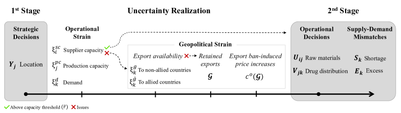
Figure 1: Sequence of events.

More specifically, the production capacity of plants $(\xi_{j}^{pc})$ is defined by two types of facility interruptions: strain $(\xi_{j}^{ps})$ and disruptions $(\xi_{j}^{pd})$. Strain refers to partial capacity interruptions. Disruption refers to the complete unavailability of the facility; we model it as $\xi_{j}^{pd}$ $\sim{\rm Bernoulli}(\rho_{j}^{pd})$ for all $j\in J$, where $\rho_{j}^{pd}$ represents the probability of having facility $j$ available. The combined effect of those two interruptions is $\xi_{j}^{pc}=\xi_{j}^{ps}\xi_{j}^{pd}$. The raw material available at each supplier ($\xi_{i}^{sc}$) is also defined by the two types of interruptions above, modeled like the capacity of plants.

The model considers the risk of export bans in every country. In practice, export bans could be implemented for several reasons; in this model, the initiating condition is based on the average global capacity for raw material production $\big{(}\sum_{i\in I}\xi_{i}^{sc}/|I|\big{)}$. If $\big{(}\sum_{i\in I}\xi_{i}^{sc}/|I|\big{)}$ is less than a threshold $\tilde{r}$, then there exists a risk that governments implement export bans; otherwise, there is no geopolitical strain. The model considers exogenous bilateral alliances between $c_{1}$ and other countries. Members of this group present less risk of being affected by their partner country’s export bans. This feature requires two random parameters related to export bans, $\xi_{k}^{g}$ for non-allies and $\xi_{k}^{\dot{g}}$ for allies. We sample $\xi_{k}^{g}$ $\sim{\rm Bernoulli}(\rho_{k})$ for all $k\in K$ and apply for non-allies of $k$, and if $\xi_{k}^{g}=0$, then sample $\xi_{k}^{\dot{g}}$ $\sim{\rm Bernoulli}(\dot{\rho_{k}})$ for all $k\in\dot{F}$ and apply to the set of allies including $c_{1}$. The terms $\rho_{k}$ and $\dot{\rho_{k}}$ represent the probability of allowing exports. There are two parameters because countries $k\in K$ have non-allies, but only some countries $k\in\dot{F}$ may have allies as well. Note that having alliances may mitigate export ban uncertainty. To illustrate, if a country $k$ allows exports to its non-allied countries ($\xi_{k}^{g,\omega}$ = 1), then it allows exports to its allies too ($\xi_{k}^{\dot{g},\omega}$ = 1). If a country $k$ bans export to its non-allied countries ($\xi_{k}^{g,\omega}$ = 0), $k$ may not restrict exports to its allies ($\xi_{k}^{\dot{g},\omega}$ can be 0 or 1). The model assumes that the joint probability distribution of the random parameters $\xi$ $:=$ $[\xi^{sc},\xi^{pc},\xi^{d},\xi^{g},\xi^{\dot{g}}]^{\top}$ is known.

By reducing the global drug supply, export bans may increase drug prices. We model this decrease as the global retained exports, $\mathcal{G}^{\omega}$ (Equation (1)). This value represents the total exogenous drug supply ($e_{k},e_{k}^{c_{1}}$) that is prevented from leaving countries due to export bans in scenario $\omega\in\Omega$. The first term refers to global exports to non-$c_{1}$ countries. The second group of terms refers to global exports to $c_{1}$ from allies and non-allies. Particularly for $c_{1}$, the first and second terms refer to exports from $c_{1}$ to non-allies and allies, respectively.

$$\mathcal{G}^{\omega}=\Bigg{(}\sum_{k\in K}e_{k}(1-\xi_{k}^{g,\omega})\Bigg{)}+\Bigg{(}\sum_{k\in\dot{F}}e_{k}^{c_{1}}(1-\xi_{k}^{\dot{g},\omega})+\sum_{k\in K\setminus\dot{F}}e_{k}^{c_{1}}(1-\xi_{k}^{g,\omega})\Bigg{)}$$ (1)

The unit cost of a shortage in country $k\in K$ is modeled with two elements: the baseline price of the drug ($c_{k}^{s}$) and the marginal price increase due to export bans ($c^{o,\omega}(\mathcal{G}^{\omega})$). The baseline price is applied to all countries, and the second is added for countries who experience export ban-induced price increases (i.e., all countries except those that both have a plant, $Y_{k}=1$, and impose an export ban, $\xi_{k}^{g,\omega}=0$). To focus on the key dynamics of ban-induced price increases, we apply a linear function for $c^{o,\omega}(\mathcal{G}^{\omega})$, i.e., $c^{o,\omega}=\beta\mathcal{G}^{\omega}$, though other expressions could be directly incorporated. Figure 2 illustrates the shortage cost mechanics for scenarios without and with export bans. Note that when there are no bans (panel (a)), the cost of unmet demand is only given by $c_{k}^{s}$, as $\mathcal{G}=0$ produces $c^{o}=0$. In panel (b), since country $c_{1}$ is open for their allies and closed to the others, and country $c_{3}$ is closed for all, the marginal increase in price is $c^{o}=\beta(e_{c_{1}}+e_{c_{3}}+e^{c_{1}}_{c_{3}})$. In this scenario, the baseline price ($c_{k}^{s}$) is applied to shortages in all countries $k\in\{c_{1},...c_{6}\}$, and the marginal price increase $(c^{o})$ is applied to shortages in all countries except those where a plant is located that impose a ban, i.e., $c_{1}$.

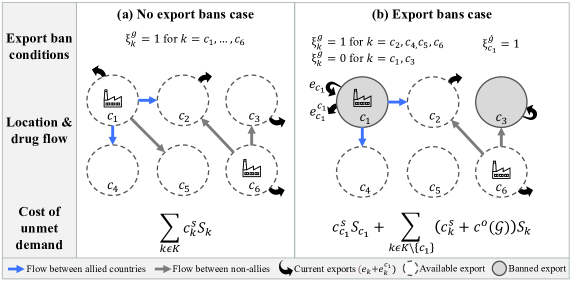
Figure 2: Composition of the unit opportunity cost for unmet demand.

3.1 Model formulation

The formulation of the stochastic program is as follows:

$$z= \min\limits_{Y}\left\{\sum_{j\in J}c_{j}^{fi}Y_{j}+\mathbb{E}_{\Omega}[Q(Y,\xi)]\right\}$$ (2a)

s.t. $$\sum_{j\in J}Y_{j}\geq 1$$ (2b)

$$Y_{j}\in\{0,1\}\quad\forall j\in J$$ (2c)

$$\mathbb{E}_{\Omega} [Q(Y,\xi)]:=\min\sum_{\omega\in\Omega}p^{\omega}\Big{(}\sum_{i\in I}\sum_{j\in J}(c_{i}^{rm}+c_{ij}^{t1})U_{ij}^{\omega}+\sum_{j\in J}\sum_{k\in K}(c_{j}^{pr}+c_{jk}^{t2})V_{jk}^{\omega}+\sum_{k\in K}(c_{k}^{s}S_{k}^{\omega}+c^{o,\omega}S_{k}^{\prime\omega})\Big{)}$$ (2d)

s.t. $$\sum_{j\in J}U_{ij}^{\omega}\leq q_{i}^{sc}\xi_{i}^{sc,\omega}\quad\forall i\in I,\omega\in\Omega$$ (2e)

$$U_{ij}^{\omega}\leq q_{i}^{sc}\xi_{i}^{sc,\omega}\xi_{i}^{g,\omega}Y_{j}\quad\forall(i,j)\in R\setminus\dot{R},\omega\in\Omega$$ (2f)

$$U_{ij}^{\omega}\leq q_{i}^{sc}\xi_{i}^{sc,\omega}\xi_{i}^{\dot{g},\omega}Y_{j}\quad\forall(i,j)\in\dot{R},\omega\in\Omega$$ (2g)

$$\sum_{k\in K}V_{jk}^{\omega}\leq q_{j}^{pc}\xi_{j}^{pc,\omega}Y_{j}\quad\forall j\in J,\omega\in\Omega$$ (2h)

$$V_{jk}^{\omega}\leq q_{j}^{pc}\xi_{j}^{pc,\omega}\xi_{j}^{g,\omega}Y_{j}\quad\forall(j,k)\in P\setminus\dot{P},\omega\in\Omega$$ (2i)

$$V_{jk}^{\omega}\leq q_{j}^{pc}\xi_{j}^{pc,\omega}\xi_{j}^{\dot{g},\omega}Y_{j}\quad\forall(j,k)\in\dot{P},\omega\in\Omega$$ (2j)

$$\sum_{j\in J}V_{jk}^{\omega}+S_{k}^{\omega}-E_{k}^{\omega}+(1-\xi_{k}^{g,\omega})e_{k}+(1-\xi_{k}^{\dot{g},\omega})e_{k}^{c_{1}}=\xi_{k}^{d,\omega}\quad\forall k\in\dot{F},\omega\in\Omega$$ (2k)

$$\sum_{j\in J}V_{jk}^{\omega}+S_{k}^{\omega}-E_{k}^{\omega}+(1-\xi_{k}^{g,\omega})e_{k}+(1-\xi_{k}^{g,\omega})e_{k}^{c_{1}}=\xi_{k}^{d,\omega}\quad\forall k\in K\setminus\dot{F},\omega\in\Omega$$ (2l)

$$\sum_{i\in I}U_{ij}^{\omega}=\sum_{k\in K}V_{jk}^{\omega}\quad\forall j\in J,\omega\in\Omega$$ (2m)

$$S_{k}^{\prime\omega}\geq S_{k}^{\omega}-\xi_{k}^{d,\omega}(1-\xi_{k}^{g,\omega})Y_{k}\quad\forall k\in J,\omega\in\Omega$$ (2n)

$$S_{k}^{\prime\omega}\geq S_{k}^{\omega}\quad\forall k\in K\setminus J,\omega\in\Omega$$ (2o)

$$U_{ij}^{\omega},V_{jk}^{\omega},E_{k}^{\omega},S_{k}^{\omega},S_{k}^{\prime\omega}\geq 0\quad\forall i\in I,j\in J,k\in K,\omega\in\Omega$$ (2p)

The objective is to minimize expected costs. In the first stage, the objective function (2a) minimizes the fixed costs plus the total expected costs of the production, distribution of drugs worldwide, and shortages. Constraint (2b) ensures that at least one plant is open, and constraints (2c) enforce the domain. In the second stage, for a finite set of scenarios $\Omega$, it minimizes the total expected cost (2d). Costs are raw materials purchase, production, transportation, and opportunity. Two types of opportunity costs are considered, $c_{k}^{s}$, the price of the drug in the country $k$, and $c^{o,\omega},$ the marginal increase in prices due to the retained exports. Raw materials purchases are limited by the available supplier capacity (2e). Flows of raw materials are limited by export bans; constraints (2f) limit flows between non-allied countries and (2g) between allies. Similarly, the production and distribution of final products are limited by the available manufacturing capacity (2h) and export bans, where constraints (2i) limit flows between non-allied countries, and (2j) between allies. The demand can be satisfied by the company’s production or by the exports held in the country because of an export ban. Constraints (2k) are the demand constraints for allies and (2l) for non-allied countries. Constraints (2m) correspond to the flow balance constraints. Constraints (2n)-(2o) define shortages in countries in which there is no manufacturing plant or that allows exports, i.e., the amount to which the price increase $c^{o,\omega}$ is applied. The auxiliary variable $S_{k}^{\prime\omega}$ takes a value of zero if a new plant is located in $k\in J$ and country $k$ is closed, i.e., if $Y_{k}$ = 1 and $\xi_{k}^{g,\omega}$ = 0, then $S_{k}^{\prime\omega}=0$; otherwise, $S_{k}^{\prime\omega}=S_{k}^{\omega}$. Finally, domain constraints for the second-stage variables are enforced (2p).

This model is subject to several assumptions. First, we consider the drug demand as price inelastic and uncorrelated because our work focuses on essential drugs that do not have substitutes (NASEM, 2022), and drug demand is mainly driven by drug’s efficacy and the number of patients (Blossey et al., 2022). The implementation of export bans is independent between countries but conditional on the risk of supplier capacity disruption; this is because of the focus on the direct (first-order) effects of export bans instead of the retaliations that governments can take against each other due to trade barriers. Changes in prices produced by a mismatch between supply and demand other than those caused by export bans are not considered, given that we are modeling marginal capacities and demand, not the entire market. We assume that supplier and production capacity strains and disruptions are independent to be consistent with previous literature (Tucker et al., 2020). We consider static location decisions because of the inherent rigidity of pharmaceutical supply chains due to regulation. Since our focus is on strategic decisions taken by a single company, we exclude granular operational decisions (e.g., inventory and drug distribution within each market) and competition; the other manufacturers stakeholders are included via the exogenous export parameters.

3.2 Structural properties

This section presents theoretical properties of the model, which help to understand its behavior and when demand will be met. Theorem 1 focuses on a country $k^{\prime}\in K$ imposing an export ban and states when retained exports will satisfy demand, i.e., forcing $V_{j{k^{\prime}}}^{\omega}=0$ for all $j\in J$. Theorem 2 states the necessary conditions for the company to satisfy demand in country $k^{\prime}\in K$ ($V_{{j^{\prime}}{k^{\prime}}}^{\omega}>0$) from manufacturing plant location, $j^{\prime}$. Here we present the case when the plant is located in an allied country of $c_{1}$ $(j^{\prime}\in J\cap F)$. Corollaries for the cases when the plant is located in the country of interest $c_{1}$ and in a non-allied country $(J\setminus\dot{F})$ are in the supplementary materials. In general, if there is production capacity in a manufacturing plant $j^{\prime}$, two things must occur for that plant to meet demand in country $k^{\prime}$. It must be economically feasible, and international trading must be allowed for flows between different countries. Finally, Theorem 3 presents the sufficient condition for the company to meet demand, assuming that Theorem 2 is satisfied. Proofs are provided in the supplementary materials.

Theorem 1 (Sufficient conditions for $V_{j{k^{\prime}}}^{\omega}=0$ $\forall j\in J$).

For a given scenario $\omega\in\Omega$, in optimality:

1. For $k^{\prime}\in K\setminus\dot{F}$, if $\xi_{k^{\prime}}^{g,\omega}=0$ and $(e_{k^{\prime}}+e_{k^{\prime}}^{c_{1}})\geq\xi_{k^{\prime}}^{d,\omega}$, then $S_{k^{\prime}}^{\omega}=0$, $E_{k^{\prime}}^{\omega}=(e_{k^{\prime}}+e_{k^{\prime}}^{c_{1}})-\xi_{k^{\prime}}^{d,\omega}$ and $V_{j{k^{\prime}}}^{\omega}=0$ $\forall j\in J$.

2. For $k^{\prime}\in\dot{F}$, if at least one condition (i)-(iii) is met, (i) ban for non-allies $\xi_{k^{\prime}}^{g,\omega}=0$ and $e_{k^{\prime}}\geq\xi_{k^{\prime}}^{d,\omega}$, or; (ii) ban for allies $\xi_{k^{\prime}}^{\dot{g},\omega}=0$ and $e_{k^{\prime}}^{c_{1}}\geq\xi_{k^{\prime}}^{d,\omega}$, or; (iii) full ban $\xi_{k^{\prime}}^{g,\omega}=0$, $\xi_{k^{\prime}}^{\dot{g},\omega}=0$, and $(e_{k^{\prime}}+e_{k^{\prime}}^{c_{1}})\geq\xi_{k^{\prime}}^{d,\omega}$. Then $S_{k^{\prime}}^{\omega}=0$ and $V_{j{k^{\prime}}}^{\omega}=0$ $\forall j\in J$. For (iii), $E_{k^{\prime}}^{\omega}=(e_{k^{\prime}}+e_{k^{\prime}}^{c_{1}})-\xi_{k^{\prime}}^{d,\omega}$.

Theorem 2 (Necessary conditions for $V_{{j^{\prime}}{k^{\prime}}}^{\omega}>0$).

Consider a scenario $\omega\in\Omega$, and conditions (i)-(iii), where:

1. Economic feasibility: $c_{k^{\prime}}^{s}+c^{o,\omega}>c_{i^{\prime}}^{rm}+c_{{i^{\prime}}{j^{\prime}}}^{t1}+c_{{j^{\prime}}}^{pr}+c_{{j^{\prime}}{k^{\prime}}}^{t2}$.

2. International trade availability for non-allies: a. $\xi_{j^{\prime}}^{g,\omega}=1$ and b. $\xi_{i^{\prime}}^{g,\omega}=1$.

3. International trade availability for allies: a. $\xi_{j^{\prime}}^{\dot{g},\omega}=1$ and b. $\xi_{i^{\prime}}^{\dot{g},\omega}=1$.

Production capacity in allied-$c_{1}$. If $\exists j^{\prime}\in\{J\cap F|Y_{j^{\prime}}=1,q_{j^{\prime}}^{pc}\xi_{j^{\prime}}^{pc,\omega}>0\}$,

1. For $k^{\prime}=c_{1}$ and $i^{\prime}\in\{I\setminus\{c_{1},j^{\prime}\}|q_{i^{\prime}}^{sc}\xi_{i^{\prime}}^{sc,\omega}>0\}$, then (i), (ii)b, and (iii)a.

2. For $k^{\prime}=c_{1}$ and $i^{\prime}=c_{1}$ with $q_{i^{\prime}}^{sc}\xi_{i^{\prime}}^{sc,\omega}>0$, then (i), (iii)a, and (iii)b.

3. For $k^{\prime}=c_{1}$ and $i^{\prime}=j^{\prime}$ with $q_{i^{\prime}}^{sc}\xi_{i^{\prime}}^{sc,\omega}>0$, then (i) and (iii)a.

4. For $k^{\prime}=j^{\prime}$ and $i^{\prime}\in\{I\setminus\{c_{1},j^{\prime}\}|q_{i^{\prime}}^{sc}\xi_{i^{\prime}}^{sc,\omega}>0\}$, then (i) and (ii)b.

5. For $k^{\prime}=j^{\prime}$ and $i^{\prime}=c_{1}$ with $q_{i^{\prime}}^{sc}\xi_{i^{\prime}}^{sc,\omega}>0$, then (i) and (iii)b.

6. For $k^{\prime}=j^{\prime}$ and $i^{\prime}=j^{\prime}$ with $q_{i^{\prime}}^{sc}\xi_{i^{\prime}}^{sc,\omega}>0$, then (i).

7. For $k^{\prime}\in K\setminus\{c_{1},j^{\prime}\}$ and $i^{\prime}\in\{I\setminus\{c_{1},j^{\prime}\}|q_{i^{\prime}}^{sc}\xi_{i^{\prime}}^{sc,\omega}>0\}$, then (i), (ii)a, and (ii)b.

8. For $k^{\prime}\in K\setminus\{c_{1},j^{\prime}\}$ and $i^{\prime}=c_{1}$ with $q_{i^{\prime}}^{sc}\xi_{i^{\prime}}^{sc,\omega}>0$, then (i), (ii)a, and (iii)b.

9. For $k^{\prime}\in K\setminus\{c_{1},j^{\prime}\}$ and $i^{\prime}=j^{\prime}$ with $q_{i^{\prime}}^{sc}\xi_{i^{\prime}}^{sc,\omega}>0$, then (i) and (ii)a.

Note: Under the no existence of export bans, condition (i) is harder to meet $(c_{k^{\prime}}^{s}>c_{i^{\prime}}^{rm}+c_{i{{}^{\prime}}j{{}^{\prime}}}^{t1}+c_{j^{\prime}}^{pr}+c_{j{{}^{\prime}}k{{}^{\prime}}}^{t2})$.

Theorem 3.

Consider a scenario $\omega\in\Omega$ and $Y_{j^{\prime}}=1$ for $j^{\prime}\in J$ with one unit of production capacity available. Suppose that for $k=k^{\prime}$ and $k=k^{\prime\prime}$, $\xi_{k}^{g,\omega}=1$ and there exists $i^{\prime}\in\{I|q_{i^{\prime}}^{sc}\xi_{i^{\prime}}^{sc,\omega}>0\}$ such that Theorem 2 is satisfied. Let $\triangle penalty_{k}^{\omega}$ be the unit marginal penalty cost for unmet demand, i.e., $\triangle penalty_{k}^{\omega}:=c_{k}^{s}+c^{o,\omega}-(c_{i^{\prime}}^{rm}+c_{{i^{\prime}}{j^{\prime}}}^{t1}+c_{j^{\prime}}^{pr}+c_{{j^{\prime}}k}^{t2})$. If $\xi_{k^{\prime}}^{d,\omega}>0$, $\xi_{k^{\prime\prime}}^{d,\omega}>0$ and $\triangle penalty_{k^{\prime}}^{\omega}>\triangle penalty_{k^{\prime\prime}}^{\omega}$, then $V_{j{k^{\prime}}}^{\omega}=1$ and $V_{j{k^{\prime\prime}}}^{\omega}=0$.

4 Solution approach

To solve the model, we integrate the Sample Average Approximation (SAA) and L-shaped methods (Algorithm 1). SAA builds stochastic programs with scenario sets of a manageable size, and the L-shaped method solves them. This allows problems with large sample spaces to be solved with low optimality gaps in a reasonable time (Santoso et al., 2005).

Input: Iteration counter $s\leftarrow 0$, $M$ replications, $N$ optimization scenarios, $N^{\prime}$ evaluation scenarios, $\epsilon_{0}$ tolerance for termination criteria.

Output: $\hat{Y}^{*}$ optimal solution, $L_{N,M}$ lower and $U_{N^{\prime}}$ upper bound estimators, and optimality gap.

1. Set $s=s+1$.

2. In parallel for $m=1,...,M,$ do 

    2.1 Generate $N$ i.i.d. scenarios of $\xi$.

    2.2 Solve the SAA problem (3) with the L-shaped method (Algorithm 2) and get $z_{N}^{m}$ and $\hat{Y}^{m}$.

$$z_{N}^{m}=\min\limits_{Y}\left\{\sum_{j\in J}c_{j}^{fi}Y_{j}^{m}+\hat{q}_{N}\right\}$$ (3)

$$\text{s.t.}\quad\eqref{C1.1}-\eqref{C1.2},\eqref{C2.1}-\eqref{C2.12}$$

    2.3 Generate $N^{\prime}$ i.i.d. scenarios of $\xi$.

    2.4 Use $\hat{Y}^{m}$ to evaluate the objective function $z_{N^{\prime}}^{m}(\hat{Y}^{m})$.

3. Select $\hat{Y}^{*}\in\operatorname*{argmin}\{z_{N^{\prime}}(\hat{Y}):\hat{Y}\in\{\hat{Y}^{1},...,\hat{Y}^{M}\}\}$.

4. Calculate $L_{N,M}\coloneqq\bar{z}_{N,M}-t_{\alpha,\nu}\hat{\sigma}_{\bar{z}_{N,M}}$ and $U_{N^{\prime}}\coloneqq z_{N^{\prime}}+z_{\alpha}\hat{\sigma}_{z_{N^{\prime}}}$ bounds of the original problem (2) using $\hat{Y}^{*}$. Where $\bar{z}_{N,M}\coloneqq\frac{1}{M}\sum_{m=1}^{M}z_{N}^{m}$, $\hat{\sigma}_{\bar{z}_{N,M}}^{2}\coloneqq\frac{1}{(M-1)M}\sum_{m=1}^{M}(z_{N}^{m}-\bar{z}_{N,M})^{2}$, $\nu=M-1$ and $t_{\alpha,\nu}$ is the $\alpha$-critical value of the t-distribution with $\nu$ degrees of freedom, and $\hat{\sigma}_{z_{N^{\prime}}}^{2}\coloneqq\frac{1}{(N^{\prime}-1)N^{\prime}}\sum_{\omega=1}^{N^{\prime}}(\sum_{j\in J}c_{j}^{fi}\hat{Y}_{j}+Q(\hat{Y},\xi^{\omega})-z_{N^{\prime}})^{2}$.

5. if $[U_{N^{\prime}}-L_{N,M}]/U_{N^{\prime}}\leq\epsilon_{0}$ then stop and report $\hat{Y}^{*}$ as the optimal solution.

else go to 1.

Algorithm 1 Integrated SAA and L-shaped decomposition methods

Input: Set of optimality cuts $\mathcal{O}\leftarrow\emptyset$, termination criteria $\epsilon\leftarrow 10^{-5}$, lower bound $lb\leftarrow 0$, and upper bound $ub\leftarrow\infty$.

Output: Optimal solution $(z_{N},\hat{Y})$ of SAA problem (3).

1. Solve master problem (4), and set $\hat{Y}$ and $lb$ as the optimal solution and objective value of (4).

$$lb= \min\limits_{Y,\theta}\left\{\sum_{j\in J}c_{j}^{fi}Y_{j}+\theta\right\}$$ (4)

s.t. $$\quad\eqref{C1.1}-\eqref{C1.2}$$

$$\quad\theta\geq\frac{1}{N}\sum_{\omega=1}^{N}(h_{o}^{\omega}-T_{o}^{\omega}Y)\pi_{o}^{\omega}\quad\forall o\in\mathcal{O}$$

2. For each scenario $\omega$, calculate $c^{o,\omega}$ and use $\hat{Y}$ to solve sub-problem (5) and get its duals $\pi^{\omega}$.

$$Q(\hat{Y},\xi^{\omega})\coloneqq\min \sum_{i\in I}\sum_{j\in J}(c_{i}^{rm}+c_{ij}^{t1})U_{ij}+\sum_{j\in J}\sum_{k\in K}(c_{j}^{pr}+c_{jk}^{t2})V_{jk}+\sum_{k\in K}(c^{o,\omega}S_{k}^{\prime}+c_{k}^{s}S_{k})$$ (5)

$$\text{s.t.}\quad\eqref{C2.1}-\eqref{C2.12}$$

3. Compute $z_{N}(\hat{Y})=\sum_{j\in J}c_{j}^{fi}\hat{Y}_{j}+\hat{q}_{N}$.

4. if $z_{N}\leq ub$ then $ub\leftarrow z_{N}$.

5. if $[(ub-lb)/ub]>\epsilon$ then  build an optimality cut $\theta\geq\frac{1}{N}\sum_{\omega=1}^{N}(h^{\omega}-T^{\omega}Y)\pi^{\omega}$, add it to the set of constraints $\mathcal{O}$, and go to 1.

else stop, return $ub$ as the optimal objective function value ($z_{N}$) and $\hat{Y}$ as the optimal solution.

Algorithm 2 L-shaped decomposition method

The SAA method builds optimization problems through an exterior sampling approach. It estimates the second-stage objective function (2d), $\mathbb{E}_{\Omega}[Q(Y,\xi)],$ by a sample average function $\hat{q}_{N}(Y)$ = $\frac{1}{N}\sum_{\omega=1}^{N}Q(Y,\xi^{\omega})$, in which the uncertainty set $\Omega$ is replaced by a set of $N$ i.i.d. sampled scenarios (Verweij et al., 2003). Solving the SAA problem (3) for $M$ independent replications, each of size $N$, we get $M$ objectives values $(z_{N}^{1},...,z_{N}^{M})$ and candidate solutions $(\hat{Y}^{1},...,\hat{Y}^{M})$. An approximate $100(1-\alpha)\%$ confidence of the statistical estimates of the lower bound $(L_{N,M})$ and upper bound $(U_{N^{\prime}})$ of the optimal objective value of (2) can be calculated as presented in Algorithm 1. In particular, $U_{N^{\prime}}$ is estimated by solving (3) with $N^{\prime}\gg N$ number of scenarios. With this procedure, a valid bound of the true gap with confidence of at least 1-2$\alpha$ is obtained. Properties of the estimators and convergence of the SAA method are explained in Kleywegt et al. (2002).

The L-shaped method (Algorithm 2), also called Benders’ decomposition, divides the two-stage program into a master problem (4) and sub-problem (5) (Santoso et al., 2005). The master problem is a relaxation of (3) in which $\hat{q}_{N}$ is approximated by a variable $\theta$ using Benders’ cuts built iteratively with the solution of $N$ subproblems (5). Since the model has complete recourse, we do not generate feasibility cuts; a single optimality cut is added in each iteration to the set of optimality cuts $\mathcal{O}$ in the form $\theta\geq\frac{1}{N}\sum_{\omega=1}^{N}(h^{\omega}-T^{\omega}Y)\pi^{\omega}$, where $\pi^{\omega}$ and $(h^{\omega}-T^{\omega}Y)$ correspond to the optimal dual multipliers and the right-hand side of the constraints associated with sub-problem (5), respectively.

5 Case study

The proposed model and solution method are implemented in a case study based on vincristine, an essential generic injectable oncology drug used to treat leukemia and Hodgkin’s and non-Hodgkin’s lymphomas. It has been in shortage in several countries, e.g., in the US (UUDIS, 2022), Colombia (Sabogal De La Pava and Tucker, 2022), and Spain (CIMA, 2022). The country of interest $c_{1}$ is the US, and we consider the set of allies $F$ as the 20 countries with Free Trade Agreements with the US (USTR, 2022); there are 11 suppliers of raw materials ($I$), 60 countries to locate plants ($J$), and 179 countries with demand ($K$). Full details on data, including methods for estimating export bans and other strain parameters, are in the supplementary materials. This case study is designed to reflect realistic dynamics of practice, study how a company may respond to geopolitical strain, and illustrate global trends in drug access as provided by a for-profit company.

We solved the model with $\alpha=1\%$ to build the bounds $(L_{N,M},U_{N^{\prime}})$, 30 replications ($M$), 100 optimization scenarios ($N$), and 2000 evaluation scenarios ($N^{\prime}$). It was implemented in Python with Gurobi v9.5.2 and a high-performance computing cluster (30 CPU cores, 46GB RAM) to solve replications. To evaluate result consistency, we performed five base case runs; we observed identical first-stage decisions and optimality gaps below 2%. Computational time averaged 3441s (57.4 min) with standard deviation of 340s (5.7 min).

First, we present the base case results in Section 5.1, reflecting current conditions. In Section 5.2, we consider the effects of emerging geopolitical risks and misspecified risk conditions. We discuss results when there are no alliances in Section 5.3. In Section 5.4, we explore pricing policies to support broader access, and in Section 5.5, we evaluate back-shoring plants to the US. Practical insights are discussed in Section 5.6, and sensitivity analyses are in the supplementary materials.

5.1 Base case results

Historical data indicates relatively low risks of export bans. We present base case conditions using this data (supplementary materials), in which the average probability of allowing exports considering all countries is 0.977, and geopolitical strain can occur when the average global capacity to produce raw materials is lower than $\tilde{r}=80\%$.

Under these conditions, three countries are selected for manufacturing capacity. Two non-allied countries are in Asia (Indonesia and Malaysia), and one US ally is in South America (Chile). Indonesia is a lower-middle income country (LMIC); Malaysia is an upper-middle income country (UMIC); and Chile is a high-income country (HIC). No low-income country (LIC) was chosen. The selected countries have the lowest fixed and production costs; their probability of allowing exports is the highest (0.99). The expected available production capacity when there is no disruption $(\mathbb{E}[\xi_{j}^{ps}])$ is 94.9% (Asian countries) and 89.1% (Chile). They have low exogenous exports of vincristine. A map with the selected countries and the distribution of drugs worldwide is in the supplementary materials.

Indonesia produces most of the drugs sent to Oceania (96%), Africa (90%), and Latin America (72%) and half to Asia (58%). Half of European volume is produced by Malaysia (53%) with 44% from Chile. The North American region (Canada and the US) is attended in 58% by Chile, a US ally. The top five raw materials suppliers are Thailand, Chile, India, the Czech Republic, and the US. The plant located in Chile purchases raw materials from its own country (76.2%) and from the US (21%), its ally.

The expected global shortage is 21%, which represents a large portion of unmet worldwide demand. The largest opportunity cost ($c^{o}$) is $11.7 when five countries applied export bans, including the top two drug exporters and all without plant locations. There is an unequal distribution of the drug regarding regions and income levels (Figure 3). The expected shortage for HICs, UMICs, LMICs, and LICs are 3.1%, 3.7%, 95.2%, and 98.7%, respectively. All LICs and most LMICs (72.5%) have an average shortage of at least 95%. Notably, one of the plant locations, Indonesia (a LMIC) has expected shortages of 88.8%. This implies that production capacity will not guarantee a domestic drug supply. Sensitivity analyses suggest that prices outweigh transportation costs in drug allocation, and the results are robust to transportation cost changes.

The disparities in drug access persist even in scenarios that have no disruptions. In one scenario without strain, no demand in LMICs and LICs is met despite excess capacity available. In a scenario with a single disruption, demand for LMICs and LICs is not met, and shortages occurred in HICs (33%) and UMICs (16%).

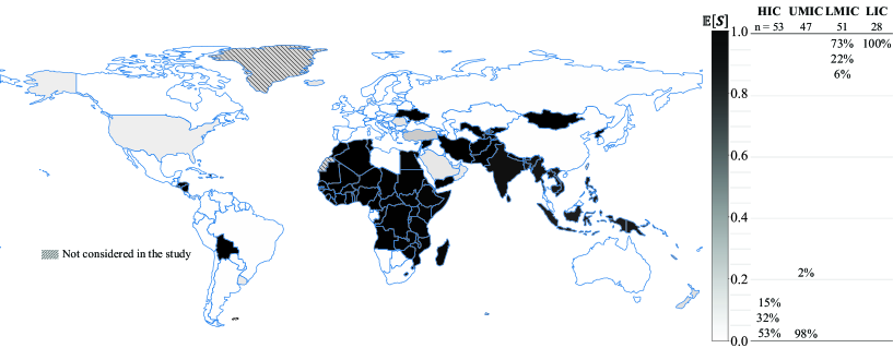
Figure 3: Expected drug shortage $(\mathbb{E}[S])$ per country and income level.

In the country of interest, $c_{1}=US$, the expected shortage is 6.7%, and one of its allies, Chile, supplies 53% of its drugs. We observe that most (81%) of its allies have expected shortages below 15% vs. half (52%) of non-allies (Table 2). Among LMICs, alliances are not sufficient to improve access; even US allies have an expected shortage of at least 95%.

Table 2: Base case proportion of countries within expected shortages $(\mathbb{E}[S])$ range.

	Countries ($K$)	Allied countries ($\dot{F}$)				Non-allied countries ($K\setminus\dot{F}$)
Expected	All	All	HIC	UMIC	LMIC	All	HIC	UMIC	LMIC	LIC
Shortage $\mathbb{E}[S]$	n = 179	21	10	7	4	158	43	40	47	28
[0 - 0.05]	41%	52%	40%	100%	-	40%	56%	98%	-	-
(0.05 - 0.1]	9%	24%	50%	-	-	8%	28%	-	-	-
(0.1 - 0.15]	4%	5%	10%	-	-	4%	16%	-	-	-
(0.15 - 0.2]	-	-	-	-	-	-	-	-	-	-
(0.2 - 0.25]	1%	-	-	-	-	1%	-	3%	-	-
⋮		⋮		⋮		⋮		⋮		⋮
(0.85 - 0.9]	2%	-	-	-	-	2%	-	-	6%	-
(0.9 - 0.95]	6%	-	-	-	-	7%	-	-	23%	-
(0.95 - 1]	36%	19%	-	-	100%	39%	-	-	70%	100%

Columns may not sum up to 100% due to rounding.

5.2 Export bans

In the wake of the COVID-19 pandemic and increasing international tensions, new geopolitical dynamics could further strain global supply chains. To evaluate potential effects of these emerging risks, we compare six contexts of geopolitical strain. Cases (0) to (3) represent known risk none, low (base case), medium, and high. Cases (4) and (5) represent misspecified plans, where the company selects locations without considering export bans, and the performance is evaluated under low- and high-risk cases. The cases are defined by two parameters: the probability that country $k\in K$ allows exports ($\rho_{k}$) and the tolerance threshold ($\tilde{r}$). Let $\rho^{base}$ represent the base case values. For country $k\in K$, $(\rho_{k},\tilde{r})$ in each case is: case 0 ($1,80\%$); case 1 ($\rho_{k}^{base},80\%$); case 2 ($\rho_{k}^{base},90\%)$; and case 3 $(0.8\rho_{k}^{base},80\%)$. In cases 4 and 5, the optimization occurs with $\rho_{k}=1$, and the evaluation occurs under low and high-risk conditions, respectively. The risk levels classifications are designated by the expected number of bans each case produces. Figure 4 presents expected drug shortages results in every country under all cases, grouping them by income level.

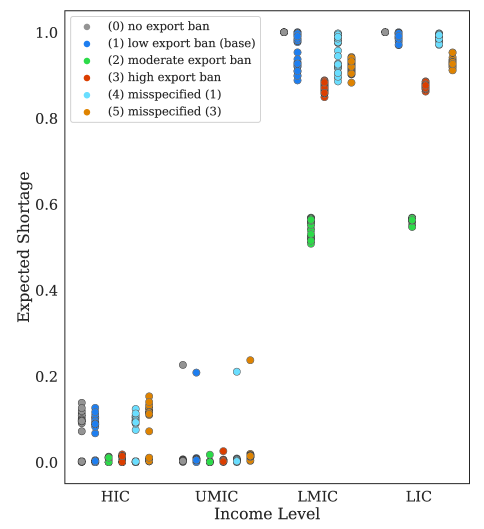
Figure 4: Expected shortage per country under increasing and misspecified geopolitical strain.

First, we consider the known risk of export bans on plant locations. Without export risk (case (0)), the selected countries are the same as the low-risk condition (case (1)). However, more countries are selected under moderate and high-risk conditions (cases (2) and (3)); these include the same three of the base case and a fourth plant (located in Russia (2) and Peru (3)). In these two configurations, the fourth plant operates as a backup which is used to meet demand under strain; it uses approximately 30% and 13% of its maximum capacity and produces only 10% and 5% of worldwide volume, respectively. The selected countries do not have high drug exports, improving market-wide diversification.

Total costs increase with increasing export bans (1.4%, 1.7%, and 2.8%, vs. case (0) for (1) to (3), respectively). Relative increases in non-shortage operational costs are 0.3%, 12%, and 2.1%, and the mean sales volume increases by 0.3%, 11.5%, and 1.8%. The total cost of shortage increases by 6% in the low-risk condition; this is because of the marginal increment in prices $c^{o}$ due to the export bans. In moderate and high-risk conditions, the total cost of shortage decreases by 52.1% and 17.5%, which could be because the company is selling more drugs, and countries that are holding their exports are satisfying their own demand, implying that the company is losing market. Compared to case (0), the sales volume increases (912, 38410, and 6039 units), but the increment does not correspond with the reduction of the global shortage (4120, 48064, and 21213 units).

We observe that export bans can reduce drug shortages. Expected global shortages are similar in cases (0) and (1) at 22% and 21% and drop to 10.8% and 17.1% with moderate- and high-risk strain, respectively. This occurs in part because an additional plant is selected in (3) and (4) that has nominally idle capacity that can be used during disruptions. For HICs, the maximum expected shortage drops from 13.8% in case (0) to 12.6%, 1.8%, and 1.3% in cases (1) to (3). In UMICs, the maximum drops to below 3% in cases (2) and (3). For LMICs and LICs, shortages decrease under cases (1) to (3), with substantial improvements in (2). This may be because the ban-induced price increases help make satisfying LMIC and LIC demand more attractive. Yet they remain very high and are always worse than in HICs and UMICs.

Our results suggest that (i) moderate and high-risk of geopolitical strain affect company location decisions, and (ii) companies may lose market because of export bans. Yet, this does not imply sales volume reduction; in fact, they are incentivized to serve new markets. In general, (iii) export bans may be a mechanism that helps to reduce shortages in the short term; however, (iv) shortages in LMICs and LICs are severe in any condition of geopolitical strain, and (v) always higher than shortages in HICs and UMICs.

Under the misspecified cases (4) and (5), we observe that low-risk conditions do not substantially affect the company’s performance nor drug shortages (vs. (1)) but do under high-risk (vs. (3)). In the high-risk case, one fewer plant is selected (as in the case without export bans (0)), indicating less resiliency. Comparing (5) with (3), the total expected cost increases by 4.6%, the fixed cost reduces by 26.3% (one plant fewer), and the expected operational cost $\hat{q}_{N}$ increases by 11.8%. The sales volume decreases by 4.1%, with a reduction in the non-shortage operational costs of 4.3%. This means the expected cost increase is due to an increase in the cost of shortage. The global expected shortage increases by 21.6%, moving from 17.1% in (3) to 20.7% in (5). US shortages also increase from 0.5% in (3) to 7.2% in (5). On average, the shortage of LICs, LMICs, UMICs, and HICs increases by 5.4, 5.0, 1.5, and 5.2 absolute percentage points (ppt) per country, respectively. These suggest that if emerging geopolitical threats worsen and exhibit high-risk conditions, ignoring export ban risks during design decisions may increase drug shortages.

5.3 Bilateral alliances

Alliances have been proposed to reduce drug shortages (The White House, 2021). To evaluate the potential effect of bilateral alliances, we performed two experiments (with low- and high-risks of export bans) in which we removed the alliances, i.e., $\xi_{k}^{\dot{g}}$ = $\xi_{k}^{g}$ $\forall k\in\dot{F}$.

Having bilateral alliances have different effects based on underlying risk conditions. In the low-risk case without alliances, the location decisions are the same as the base case, expected costs increase by 0.6%, sales volume declines by 0.3% with an equal reduction in the non-shortage operational costs, and total cost of shortage increases by 3.7%. In the high-risk case, one of selected locations (South Korea) is different than in the alliances model (Peru, case (3)), though both are US allies. This change increases expected costs by 2.7%. In detail, the fixed cost increases by 3.4%, sales volume reduces by 0.5% without changes in the non-shortage operational costs, and shortage cost increases by 12.4%. As a result, alliances have minimal impact in a low-risk case, while under high-risk, they may affect supply chain decisions and economic performance. In both experiments, bilateral alliances produce small changes in expected shortages (both 0.3 ppt increase). The biggest decreases in a particular country are 1.5 ppt (low-risk) and 3 ppt (high-risk), while the biggest increases are 0.3 ppt (low-risk) and 0.5 ppt (high-risk). These results suggest that bilateral cooperation agreements to mitigate geopolitical strain do not strongly impact drug shortages. Agreements may have some impact on drug distribution under high-risk conditions.

5.4 Pricing policies and impacts on LMICs and LICs

The results that reflect current conditions (Section 5.1) suggest an inequitable distribution of the drug where LMICs and LICs have high shortages. This is consistent with current trends observed in practice (Suda et al., 2022) due to the price differentials (Martei et al., 2020). Model results indicate that the low prices in LMICs and LICs are not sufficient to cover the cost of producing and distributing the drugs, even when capacity is available.

To evaluate the potential of pricing policies to promote access in LMICs and LICs, we run three experiments. Each changes the parameter $c_{k}^{s}$, i.e., the baseline opportunity cost for unmet demand in country $k\in K$ (price). In the first, the policy is not to use differential pricing; all countries have the same price (set equal to the US base). In the second and third experiments, we increase LMIC and LIC baseline prices by 50% and 100%, respectively. The prices for UMICs and HICs are set to their base values. The latter two represent policies in which governments or non-profit institutions subsidize part of the price, similar to the financial support of GAVI for LIC-LMIC vaccine procurement.

Table 3: Expected shortage by income level under different pricing policies.

Experiment	HIC	UMIC	LMIC	LIC
Base (1)	3.1%	3.7%	95.2%	98.7%
No differential prices	3.2%	1.1%	0.3%	0.1%
50% LIC-LMIC	0.2%	0.3%	9.0%	10.4%
100% LIC-LMIC	0.3%	1.8%	7.1%	9.5%

In each experiment, the selected locations are the same (Indonesia, Malaysia, Chile (US-allied), and Thailand). The policies make it economically feasible to open one extra plant (Thailand), compared to base case, which improves supply chain resilience. The expected costs increase by 3.4%, 1.7%, and 2.5%, respectively. The sales volume increases by 24%, 24.4%, and 24.5%, and the total cost of shortage decreases by 77.9%, 87.1%, and 83.7%.

Global drug access substantially improves in each experiment (Table 3). The expected global drug shortage is 2.2% for the experiment with equal prices and 2% with LIC-LMIC price supplements (vs. 21% at base case). Subsidizing LMIC and LIC prices also reduces shortages in HICs and UMICs. The maximum expected drug shortage that occurred in a country for every experiment was 12.1%, 11%, and 10.6%. Our results suggest that pricing policies may be effective at mitigating shortages in LMICs and LICs.

5.5 Back-shoring

Finally, we study the potential effects of back-shoring, a policy promoted by governments, including the US (The White House, 2021). To enforce back-shoring, we require the company to open a plant in the US by adding the constraint $Y_{c_{1}}=1$ to program (4). We study this under strain cases (1) and (3). As a secondary analysis, we consider the case where the US plant is of higher quality than base case, i.e., decrease disruption rate ($\xi_{US}^{pd}$) by 50% (moderate) and 75% (high) and set operational quality ($\xi_{US}^{ps}$) to the worldwide highest.

When back-shoring to the US, keeping the base case plant quality requirements, the selected countries are Indonesia, Malaysia, Chile, and the US, for both export ban risks. The US manufacturing plant possesses around 5% of the total production, and it uses 14% of its manufacturing capacity while the others operate above 86%. This is because the US plant has higher production costs, and it is only used as a backup to mitigate possible disruptions in the other selected manufacturing plants or the risk of export bans.

With back-shoring, US shortages are expected to be nearly eliminated for low-risk geopolitical strain (shortages of 0.3% vs. base case of 6.7%). In a high-risk setting, US shortages are nearly the same with required back-shoring (0.8%) vs. not (0.5%). Although there is a plant in the US, Chile supplies the majority of US drugs in expectation, 59% (low-risk) and 57% (high-risk). The US supplies 3.3% (low-risk) and 3.7% (high-risk) of its drugs. Moreover, most of the destinations of the drugs sent by the US are HICs, 89.5% (low-risk) and 88.2% (high-risk). These are reflective of the high production cost in the US. The inequities in drug distribution are still present, though the gap is reduced in the low-risk condition. For this case, all LMICs and LICs have an expected shortage between 85% and 90% (before, it was at least 95%), whereas in HICs and UMICs the expected shortage is lower than 5%. Both US allies and non-allies reduced their expected shortages; however, reductions were slightly higher in allied HICs and LMICs. In the high-risk condition, the shortage had similar results to high-risk case (3) of Section 5.2.

In the secondary set of experiments with higher quality US plants, we observe that surprisingly, improving the quality of the production process does not affect the company’s economic performance, location decisions, nor global shortages in expectation. There are some benefits to US shortages specifically. In the low-risk case, the US shortage was 0.3% in both quality scenarios, and in the high-risk case, the US shortage was 0.3% and 0.4%; each half of the shortages with back-shoring only (0.8%). Shortages in allied countries in expectation did not change, even when allied countries have a greater chance of not being affected by export bans when locating a plant in the US. This implies adding redundancy when requiring back-shoring has a higher impact than improving quality at a single plant.

5.6 Practical insights

Several recent events have increased geopolitical strain, e.g., the export bans implemented during the COVID-19 pandemic and the Ukraine-Russia war. This work studies the effects of such restrictions on supply chain design and drug shortages.

Our results surprisingly suggest that in the short-term, export bans may reduce shortages in the country imposing the ban and could reduce shortages in multiple countries. A moderate risk of export bans may provide sufficient stress on the system to improve resilience. Different export ban risks may produce different supply chains, increasing the supply chain’s expected costs even when the shortage cost is reduced. Companies may not be planning for geopolitical strain; our findings indicate that the designed supply chain under misspecified export ban risk underperforms when there are high risks of export bans. This highlights a need for companies to evaluate risk levels during planning.

Our study includes bilateral alliances with a country of interest to investigate their potential to mitigate geopolitical strain. These alliances show minor improvements in the company’s economic performance and shortages in expectation. Under high-risk conditions, it produces changes in location decisions. Given the current long and global supply chain structures, it is possible that unconsidered multi-country alliances may be more effective.

Pharmaceutical companies are for-profit organizations. In search of efficient operations, e.g., reducing costs, they can make decisions that produce inequities between markets. In our results, LICs and LMICs have high drug shortages in all geopolitical risk cases considered, in contrast to HICs and UMICs, whose shortages are relatively low. We show that with pricing policies, access to drugs in LICs and LMICs could be substantially improved. There are also side effects leading to improved shortages for HICs and UMICs.

We evaluate the policy of back-shoring manufacturing activities to the US. We find that this strategy is not optimal, but it does not have substantial negative effects. Government incentives could be used to make back-shoring economically attractive for companies. The redundancy of a domestic manufacturing plant for low-risk case decreases domestic US shortages to 0.3%, essentially equivalent effect as high-risk geopolitical risk. The US plant is used as a backup rather than primary plant because of its high production costs.

The focus of the model is to give insights into the dynamics of practice but not actual shortages and behaviors. Limitations include the estimation of data through publicly available sources (see supplementary materials) that may not precisely reflect confidential information related to demand, costs, and capacities. We assume that capacity disruptions are independent between countries. Export bans do not include retaliations. Competition is only implicitly included via exogenous export parameters and market loss with retained exports. The model does not consider economic features of international trade to focus on the geopolitical dynamics. Finally, drug shortages are reported in the context of demand met by a company optimizing its costs; it may also be met with other mechanisms.

6 Conclusion

Globalization has created interdependencies and increased supply chain vulnerabilities to emerging geopolitical risks. To address unstudied questions of geopolitical strain, this work proposes a two-stage stochastic program to study the global supply chain design problem under export bans in the pharmaceutical industry. We focus on determining how geopolitical strain, bilateral alliances between nations, pricing, and back-shoring policies may affect the company’s economic performance, design decisions, and shortages globally and by income level classification. Our results suggest the complexity of providing access to LMICs and LICs where base case prices are not sufficiently attractive. We observe that companies may be incentivized to meet demand in those markets with price supplements. They may also reduce shortages in HICs and UMICs. Moderate export bans may provide sufficient stress on the system to enhance resilience.

This model provides a foundation for the inclusion of geopolitical strain in pharmaceutical supply chain design. It also calls attention to studying the effects of geopolitical strain on global supply chains in other industries. Future work could incorporate other international economic features of global trade, such as taxes, exchange rates, and transfer prices. In addition, export bans are one way to restrict international trading; future work could be related to integrating other strains, such as export quotas, licensing, and duties.

Data availability statement

The authors confirm that the data sources and descriptions of estimations are available within the article and its supplementary materials. In particular, the complete database is currently available upon reasonable request, and upon acceptance of the article, it will be made publicly available via GitHub.

Supplementary Materials for “Effects of Geopolitical Strain on Global Pharmaceutical Supply Chain Design and Drug Shortages”

Martha L. Sabogal De La Pava and Emily L. Tucker

Section 1 presents further structural properties of the model and a summary of Theorem 2 and its corollaries. Section 2 includes proofs of all structural properties presented. Detail on data used for stochastic and deterministic parameters of the model are presented in Sections 3 and 4, respectively. Sensitivity analyses and additional results are in Section 5.

1 Further structural properties

This section presents additional model properties that relate to the company’s satisfaction of demand. One case (when the plant is located in an allied country of $c_{1}$) is presented in the main text as Theorem 2. In this supplemental section, we present two corollaries which state the necessary conditions for $V_{{j^{\prime}}{k^{\prime}}}^{\omega}>0$ for the two other cases of $j^{\prime}$, i.e., when the plant is located in the country of interest $c_{1}$ (Corollary 1) and in a non-allied country (Corollary 2). To synthesize the results of Theorem 2 and the corollaries, we present all the necessary conditions for each case in Table 1.

Corollary 1.

Production capacity in $c_{1}$. If $Y_{c_{1}}=1$ and $q_{c_{1}}^{pc}\xi_{c_{1}}^{pc,\omega}>0$,

1. For $k^{\prime}\in F$ and $i^{\prime}\in\{I\setminus\dot{F}|q_{i^{\prime}}^{sc}\xi_{i^{\prime}}^{sc,\omega}>0\}$, then (i),(ii)b and (iii)a.

2. For $k^{\prime}\in F$ and $i^{\prime}\in\{I\cap F|q_{i^{\prime}}^{sc}\xi_{i^{\prime}}^{sc,\omega}>0\}$, then (i),(iii)a and (iii)b.

3. For $k^{\prime}\in F$ and $i^{\prime}=c_{1}$ with $q_{i^{\prime}}^{sc}\xi_{i^{\prime}}^{sc,\omega}>0$, then (i) and (iii)a.

4. For $k^{\prime}=c_{1}$ and $i^{\prime}\in\{I\setminus\dot{F}|q_{i^{\prime}}^{sc}\xi_{i^{\prime}}^{sc,\omega}>0\}$, then (i) and (ii)b.

5. For $k^{\prime}=c_{1}$ and $i^{\prime}\in\{I\cap F|q_{i^{\prime}}^{sc}\xi_{i^{\prime}}^{sc,\omega}>0\}$, then (i) and (iii)b.

6. For $k^{\prime}=c_{1}$ and $i^{\prime}=c_{1}$ with $q_{i^{\prime}}^{sc}\xi_{i^{\prime}}^{sc,\omega}>0$, then (i).

7. For $k^{\prime}\in K\setminus\dot{F}$ and $i^{\prime}\in\{I\setminus\dot{F}|q_{i^{\prime}}^{sc}\xi_{i^{\prime}}^{sc,\omega}>0\}$, then (i), (ii)a and (ii)b.

8. For $k^{\prime}\in K\setminus\dot{F}$ and $i^{\prime}\in\{I\cap F|q_{i^{\prime}}^{sc}\xi_{i^{\prime}}^{sc,\omega}>0\}$, then (i), (ii)a and (iii)b

9. For $k^{\prime}\in K\setminus\dot{F}$ and $i^{\prime}=c_{1}$ with $q_{i^{\prime}}^{sc}\xi_{i^{\prime}}^{sc,\omega}>0$, then (i) and (ii)a.

Corollary 2.

Production capacity in non-allies. If $\exists j^{\prime}\in\{J\setminus\dot{F}|Y_{j^{\prime}}=1,q_{j^{\prime}}^{pc}\xi_{j^{\prime}}^{pc,\omega}>0\}$,

1. For $k^{\prime}\in K\setminus\{j^{\prime}\}$ and $i^{\prime}\in\{I\setminus\{j^{\prime}\}|q_{i^{\prime}}^{sc}\xi_{i^{\prime}}^{sc,\omega}>0\}$, then (i), (ii)a, and (ii)b.

2. For $k^{\prime}\in K\setminus\{j^{\prime}\}$ and $i^{\prime}=j^{\prime}$ with $q_{i^{\prime}}^{sc}\xi_{i^{\prime}}^{sc,\omega}>0$, then (i) and (ii)a.

3. For $k^{\prime}=j^{\prime}$ and $i^{\prime}\in\{I\setminus\{j^{\prime}\}|q_{i^{\prime}}^{sc}\xi_{i^{\prime}}^{sc,\omega}>0\}$, then (i) and (ii)b.

4. For $k^{\prime}=j^{\prime}$ and $i^{\prime}=j^{\prime}$ with $q_{i^{\prime}}^{sc}\xi_{i^{\prime}}^{sc,\omega}>0$, then (i).

Table 1: Summary of necessary conditions for $V_{{j^{\prime}}{k^{\prime}}}^{\omega}>0$.

$j^{\prime}|Y_{j^{\prime}}=1,q_{j^{\prime}}^{pc}\xi_{j^{\prime}}^{pc,\omega}>0$	$k^{\prime}$	$i^{\prime}$$|q_{i^{\prime}}^{sc}\xi_{i^{\prime}}^{sc,\omega}>0$	Necessary conditions
$j^{\prime}\in J\cap F$	$k^{\prime}=c_{1}$	$i^{\prime}\in I\setminus\{c_{1},j^{\prime}\}$	$(i),(ii)b,(iii)a$
$j^{\prime}\in J\cap F$	$k^{\prime}=c_{1}$	$i^{\prime}=c_{1}$	$(i),(iii)a,(iii)b$
$j^{\prime}\in J\cap F$	$k^{\prime}=c_{1}$	$i^{\prime}=j^{\prime}$	$(i),(iii)a$
$j^{\prime}\in J\cap F$	$k^{\prime}=j^{\prime}$	$i^{\prime}\in I\setminus\{c_{1},j^{\prime}\}$	$(i),(ii)b$
$j^{\prime}\in J\cap F$	$k^{\prime}=j^{\prime}$	$i^{\prime}=c_{1}$	$(i),(iii)b$
$j^{\prime}\in J\cap F$	$k^{\prime}=j^{\prime}$	$i^{\prime}=j^{\prime}$	$(i)$
$j^{\prime}\in J\cap F$	$k^{\prime}\in K\setminus\{c_{1},j^{\prime}\}$	$i^{\prime}\in I\setminus\{c_{1},j^{\prime}\}$	$(i),(ii)a,(ii)b$
$j^{\prime}\in J\cap F$	$k^{\prime}\in K\setminus\{c_{1},j^{\prime}\}$	$i^{\prime}=c_{1}$	$(i),(ii)a,(iii)b$
$j^{\prime}\in J\cap F$	$k^{\prime}\in K\setminus\{c_{1},j^{\prime}\}$	$i^{\prime}=j^{\prime}$	$(i),(ii)a$
$j^{\prime}=c_{1}$	$k^{\prime}\in F$	$i^{\prime}\in I\setminus\dot{F}$	$(i),(ii)b,(iii)a$
$j^{\prime}=c_{1}$	$k^{\prime}\in F$	$i^{\prime}\in I\cap F$	$(i),(iii)a,(iii)b$
$j^{\prime}=c_{1}$	$k^{\prime}\in F$	$i^{\prime}=c_{1}$	$(i),(iii)a$
$j^{\prime}=c_{1}$	$k^{\prime}=c_{1}$	$i^{\prime}\in I\setminus\dot{F}$	$(i),(ii)b$
$j^{\prime}=c_{1}$	$k^{\prime}=c_{1}$	$i^{\prime}\in I\cap F$	$(i),(iii)b$
$j^{\prime}=c_{1}$	$k^{\prime}=c_{1}$	$i^{\prime}=c_{1}$	$(i)$
$j^{\prime}=c_{1}$	$k^{\prime}\in K\setminus\dot{F}$	$i^{\prime}\in I\setminus\dot{F}$	$(i),(ii)a,(ii)b$
$j^{\prime}=c_{1}$	$k^{\prime}\in K\setminus\dot{F}$	$i^{\prime}\in I\cap F$	$(i),(ii)a,(iii)b$
$j^{\prime}=c_{1}$	$k^{\prime}\in K\setminus\dot{F}$	$i^{\prime}=c_{1}$	$(i),(ii)a$
$j^{\prime}\in J\setminus\dot{F}$	$k^{\prime}\in K\setminus\{j^{\prime}\}$	$i^{\prime}\in I\setminus\{j^{\prime}\}$	$(i),(ii)a,(ii)b$
$j^{\prime}\in J\setminus\dot{F}$	$k^{\prime}\in K\setminus\{j^{\prime}\}$	$i^{\prime}=j^{\prime}$	$(i),(ii)a$
$j^{\prime}\in J\setminus\dot{F}$	$k^{\prime}=j^{\prime}$	$i^{\prime}\in I\setminus\{j^{\prime}\}$	$(i),(ii)b$
$j^{\prime}\in J\setminus\dot{F}$	$k^{\prime}=j^{\prime}$	$i^{\prime}=j^{\prime}$	$(i)$

2 Proofs

Theorem 1

Proof.

For part (I), considering the theorem conditions and rewriting constraint (2l), $\sum_{j\in J}V_{jk}^{\omega}+S_{k}^{\omega}-E_{k}^{\omega}=\xi_{k}^{d,\omega}-(e_{k}+e_{k}^{c_{1}})$. Note that the right-hand side would be negative or zero, and by domain constraints (2p) and the sense of the objective function (2d), in optimality $\sum_{j\in J}V_{jk}^{\omega}=0\Rightarrow V_{jk}^{\omega}=0$ $\forall j\in J$, $S_{k}^{\omega}=0$ and $E_{k}^{\omega}=(e_{k}+e_{k}^{c_{1}})-\xi_{k}^{d,\omega}$. Part (II) is proven similarly with constraint (2k) in place of (2l). ∎

Theorem 2

Proof.

Production capacity in $allied-c_{1}$. Considering the premises presented for parts (I)-(VI), condition (i) comes from demand constraints (2k), domain constraints (2p), flow balance constraints (2m) and the sense of the objective function (2d); condition (iii)a comes from constraints (2j); and conditions (ii)b and (iii)b from constraints (2f) and (2g), respectively. For parts (VII)-(IX), condition (i) comes from demand constraints (2k)-(2l), domain constraints (2p), flow balance constraints (2m) and the objective function (2d); condition (ii)a comes from constraints (2i); and conditions (ii)b and (iii)b from constraints (2f) and (2g), respectively. Note that flows with the same origin and destination, i.e., $V_{{j^{\prime}}{k^{\prime}}}^{\omega}$ for ${k^{\prime}}={j^{\prime}}$ and $U_{{i^{\prime}}{j^{\prime}}}^{\omega}$ for ${i^{\prime}}={j^{\prime}}$ are not included in (2i)-(2j) and (2f)-(2g), respectively. Therefore, international trade availability conditions do not apply to those cases. ∎

Corollary 1

Proof.

Production capacity in $c_{1}$. Considering the premises presented in parts (I)-(VI), condition (i) comes from demand constraints (2k), domain constraints (2p), flow balance constraints (2m) and the sense of the objective function (2d); condition (iii)a comes from constraints (2j); and conditions (ii)b and (iii)b from constraints (2f) and (2g), respectively. For parts (VII)-(IX), condition (i) comes from demand constraints (2l), domain constraints (2p), flow balance constraints (2m) and the sense of the objective function (2d); condition (ii)a comes from constraints (2i); and conditions (ii)b and (iii)b from constraints (2f) and (2g), respectively. Note that $V_{{c_{1}}{c_{1}}}^{\omega}$ is not limited by (2i)-(2j) and $U_{{c_{1}}{c_{1}}}^{\omega}$ is not included in (2f)-(2g). Therefore, international trade availability conditions do not apply to those cases. ∎

Corollary 2

Proof.

Production capacity in non-allies. Considering the premises presented in parts (I)-(IV), condition (i) comes from demand constraints (2k)-(2l), domain constraints (2p), flow balance constraints (2m) and the sense of the objective function (2d); condition (ii)a comes from constraints (2i); and condition (ii)b from constraints (2f). By the same elements of the model, when at least one of the conditions does not hold, then $V_{{j^{\prime}}{k}^{\prime}}^{\omega}=0$. Note that $V_{{j^{\prime}}{k^{\prime}}}^{\omega}$ is not limited by (2i) when ${k^{\prime}}={j^{\prime}}$, and $U_{{i^{\prime}}{j^{\prime}}}^{\omega}$ is not limited by (2f) when ${i^{\prime}}={j^{\prime}}$, therefore conditions (ii)a and (ii)b do not apply for those cases respectively. ∎

Theorem 3

Proof.

Since Theorem 2 is satisfied, we know that $V_{{j^{\prime}}{k^{\prime}}}^{\omega}$ and $V_{{j^{\prime}}{k^{\prime\prime}}}^{\omega}$ can be greater than zero, and that $\triangle penalty_{k^{\prime}}^{\omega}>\triangle penalty_{k^{\prime\prime}}^{\omega}>0$. By the sense of the objective function (2d) at optimality $V_{{j^{\prime}}{k^{\prime}}}^{\omega}=1$ and $V_{{j^{\prime}}{k^{\prime\prime}}}^{\omega}=0$. ∎

3 Stochastic parameters

3.1 Demand

Demand in every country $(\xi_{k}^{d})$ was assumed to be normally distributed, consistent with other works, e.g., s-Zandkarimkhani2020. The mean was estimated as follows: first, we got the total number of new people with cancer per country using: (i) the cancer incidence rate of Hodgkin lymphoma, Leukemia, and Non-Hodgkin lymphoma, some of the cancers treated with vincristine s-IARC-WHO2020; and (ii) the population in every country from s-Worldometer2020, both databases from 2020. Second, we estimated the amount of drug required per person (ml/person) using the US vincristine demand presented by s-Tucker2020 and people in the US with the relevant cancers calculated in the previous step. Finally, since cancer treatments are not completely available in lower-income countries s-Dhyani2022, the demand of developing countries was adjusted accordingly with the information presented in s-Suda2022 for the Antineoplastic and Immunomodulators drug category. To calculate the standard deviations, we used the coefficient of variation for developed and developing countries calculated from s-Suda2022 under the same drug category and the previously estimated means. Here, we assumed that all patients require the same amount of drug for their treatment.

3.2 Export bans

We assumed $\xi_{k}^{g}$ $\sim{\rm Bernoulli}(\rho_{k})$ for all $k\in K$ and $\xi_{k}^{\dot{g}}$ $\sim{\rm Bernoulli}(\dot{\rho_{k}})$ for all $k\in\dot{F}$; where $\rho_{k}$ and $\dot{\rho_{k}}$ represent the probability of allowing exports to non-allies and allies, respectively. We estimated (1 - $\rho_{k}$) using the Quantitative Restrictions database from 2012-2022 s-WTO2022a and the Trade Monitoring database s-WTO2022b, considering the export prohibitions of pharmaceutical products, and removing restrictions based on special agreements such as the Chemical Weapons Convention, Convention on International Trade in Endangered Species of Wild Fauna and Flora, among others. Regarding $\dot{\rho_{k}}$, we assumed $\dot{\rho_{k}}$ = 0.85 for countries in the databases. For countries with no records on the databases, that is, countries that have not implemented export bans, we used $\rho_{k}$ = 0.99 and $\dot{\rho_{k}}$ = 0.9.

3.3 Capacity strains

$\xi_{i}^{ss}$ and $\xi_{j}^{ps}$ represent strains that affect manufacturing processes for suppliers $i\in I$ and plants $j\in J$. We calculated probability mass functions, $p(n)$ for $n=$ 0.7, 0.75, 0.8, 0.85, 0.9, 0.95,1, using histograms based on the capacities utilization databases s-FRED2022,s-TradingEconomics2022. For countries with information in the databases, specific distributions were obtained (USA, CAN, ZAF, NGA, IND, CHN, BRA, ARG, COL, AUS, and NZL); for the others, an average per continent was used. We applied separate values for North, Central, and South America.

3.4 Disruptions

We assumed $\xi_{i}^{sd}$ $\sim{\rm Bernoulli}(\rho_{i}^{sd})$ for all $i\in I$ and $\xi_{j}^{pd}$ $\sim{\rm Bernoulli}(\rho_{j}^{pd})$ for all $j\in J$; where $\rho_{i}^{sd}$ and $\rho_{j}^{pd}$ represent the probability of having facility $i$ and $j$ available, respectively. These probabilities were estimated using the average time to disruption and recovery presented by s-Tucker2020. The same values were used for every facility.

4 Deterministic parameters

All costs were adjusted to the year 2021 using the consumer price index for prescription drugs in the US published on the Statista website s-Statista2022.

4.1 Costs for opening and operating manufacturing plants (fixed costs) and production costs

For 25 countries, we estimated the fixed cost $(c_{j}^{fi})$ and production costs $(c_{j}^{pr})$ of manufacturing plants in each country using the US costs presented by s-Tucker2020 as a baseline and the Global Manufacturing Cost-Competitiveness Index of 2019 s-WorldBank2020. We calculated the performance of these countries relative to the US index. For the other countries, we used the Ease of Doing Business score of 2019 s-BCG2020, and the comparison was made using the index of a referee country in every continent from the previous 25.

4.2 Raw material cost

We used the same cost for all suppliers, taking the raw material cost of vincristine from s-Tucker2020.

4.3 Transportation costs

Transportation costs $(c_{ij}^{t1},c_{jk}^{t2})$ were estimated using the International Merchandise Trade - Transportation Costs data published by the United Nations Conference on Trade and Development s-UNCTADstat2016. In particular, we took the CIF-FOB margins per kg and 10000 km for all modes of transport and considered drugs as a commodity. Ten databases were available with cost information for the year 2016. We averaged across the ten databases to estimate an average transportation cost per ml per 10000 km for the origins and destinations of eight regions (Africa, Asia, North America, Caribbean, Central America, South America, Oceania, and Europe). Using the calculated transportation costs per unit distance between the respective regions ($/ml 10k km) and the distance between major cities of every country, we calculated the unit transportation cost between countries in $/ml. Since we used CIF-FOB margins, if the origin and destination are the same countries, the cost is $0.

4.4 Opportunity costs

Drug prices were used as the opportunity cost $c_{k}^{s}$ of unmet demand in every country. For OECD countries, we used the International Prescription Drug Price Comparisons for unbranded generics without biologics s-RR-2956-ASPEC and the US price presented by s-Tucker2020 as a baseline. For the rest of the countries, we used the median generic prices for vincristine presented by s-Martei2020 per country income level classification.

The opportunity cost $c^{o}$ was assumed to be a linear function of the exogenous retained exports produced by export bans. The slope of the linear function was 0.00003, estimated considering as $\Delta$prices 50% and $\Delta$shortages the US mean demand 90000 ml. The FDA has used 50% as a referent value to analyze shortages of drugs that experience sustained price increases after a shortage occurs s-FDA2019.

4.5 Production capacity

Manufacturing plants’ and suppliers’ capacities $(q_{j}^{pc},q_{i}^{sc})$ were assumed to be 120000 ml and 100000 ml, respectively.

4.6 Exports

Reference values for drug exports of vincristine $(e_{k}$,$e_{k}^{c_{1}})$ by volume and per country were constructed as follows: first, using the s-UNComtradeDatabase2019 and considering HS code 300449 - medicaments containing alkaloids or derivatives, we calculated the percentage of participation of every country in the international trade. Note that vincristine is a vinca alkaloid s-Dhyani2022. Second, we defined the total global trade of vincristine using the global prevalence of the cancers mentioned previously (from the International Agency for Research on Cancer website) and following the same procedure implemented to get the mean demand. Finally, we multiply the participation percentage of each country in the international trade by the total exports.

5 Sensitivity analyses and additional results

5.1 Sensitivity analysis of transportation costs

Transportation costs are the largest component of the logistics costs of an enterprise s-Rodrigue2020. To evaluate the effects of higher transportation costs on the performance and decisions of the company, we ran an experiment with doubled values for $c_{ij}^{t1}$ and $c_{jk}^{t2}$ under the base case conditions. As a result, location decisions were the same (Indonesia, Malaysia, and Chile). The expected costs increased by 0.1%, and the sales volume decreased by 0.3%, with a decrease in non-shortage operational costs by 0.1%. The penalty cost for unmet demand increased by 0.8%. The expected global shortage increased 0.3 ppt (moving from 21% to 21.3%). Regarding the expected shortage per income level, for HICs, UMICs, and LMICs, the shortage increased by 0.3, 0.1, and 0.2 ppt, while for LICs, the shortage decreased by 0.1 ppt. In particular, for the US, the expected shortage increased by 0.7 ppt, going from 6.7% to 7.4%. These show that our results are robust to changes in transportation costs.

5.2 Sensitivity analysis of the risk of export ban for specific countries

In the study of export ban risks (main text section 5.2), the selection of locations under no- and low-risk of export bans (cases (0) and (1)) were the same. The locations of Indonesia, Malaysia, and Chile represent a low risk of geopolitical strain and also provide the best economic performance. We ran an experiment by swapping the probability of allowing exports of these three countries with the three lowest $\rho_{k}$ of our case study. Here we kept the low-risk context, the average probability of allowing exports is 0.9767 per country. Particularly, $\rho_{Indonesia}^{new}$ =$\rho_{Australia}^{base}$, $\rho_{Malaysia}^{new}$ =$\rho_{India}^{base}$, $\rho_{Chile}^{new}$ =$\rho_{Albania}^{base}$, and $\rho_{k}=0.99$ for $k=Australia,India,Albania$.

As a result, we observed that even under low-risk of export bans, optimal location decisions can be affected. In this experiment, Chile (US-allied) is again selected, and two non-allied countries, Thailand, an Asian UMIC, and Greece, a European HIC. The global shortage is 21.4%, similar to the base case results (21%). The shortage in the selected countries is lower than 1% because they are countries with high incomes, different from the base case where Indonesia (a LMIC) was selected to invest in manufacturing capacity, and its shortage was high (88.8%). The gap related to drug shortages between countries with higher and lower incomes still persists under this configuration; for HICs, UMICs, LMICs, and LICs, the expected shortage was 3.2%, 4.1%, 96.7%, and 99.7%, respectively. This experiment also shows the importance of properly estimating the geopolitical risks of every country, given that it can affect supply chain design decisions.

5.3 Base case additional results

For the base case analysis (main text Section 5.1), Figure 1 shows the selected countries and the distribution of drugs worldwide. Note that the greater the intensity and thickness of the arrows, the greater the flow.

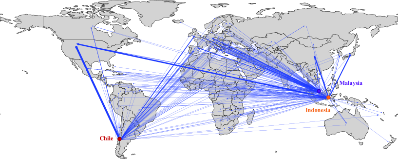
Figure 1: Base case - selected countries and drug distribution.

5.4 Pricing policies additional results

The effect of the studied pricing schemes (main text Section 5.4) on the expected drug shortage per country grouped by income level is presented in Figure 2. Figure 3 presents results for the pricing policy subsidizing 50% LIC-LMIC prices. Particularly, it shows the expected shortage per country and the proportion of countries within the expected shortage range.

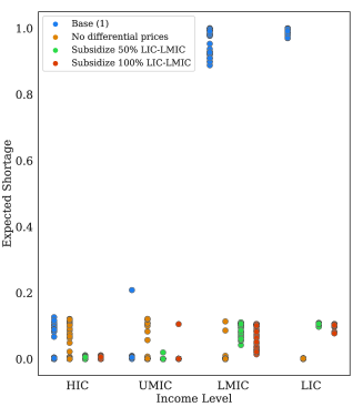
Figure 2: Expected drug shortage under different pricing schemes.

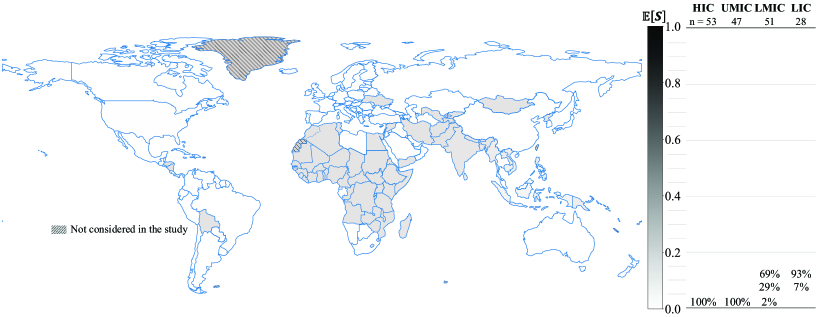
Figure 3: Expected drug shortage $(\mathbb{E}[S])$ under subsidize 50% LIC-LMIC price policy.

5.5 Back-shoring additional results

In the main text Section 5.5, we present results when the back-shoring policy is required under both geopolitical strain conditions (low- and high-risk) and under three manufacturing plant quality levels (base case, moderate and high quality). Data used in the experiments and additional results are presented in this supplementary section. For the moderate and high-quality experiments, we improved the uncertainty parameters $\xi_{US}^{pd}$ and $\xi_{US}^{ps}$ simultaneously. Specifically, for $\xi_{US}^{pd}$ we decreased the rate of disruptions by 50% (moderate-quality) and 75% (high-quality), resulting in probabilities of internal disruptions $\rho_{US}^{pd}=0.9861$ and $\rho_{US}^{pd}=0.9930$, respectively. In addition, for $\xi_{US}^{ps}$ we improved the expected value of the strains that affect the production capacity of the US, i.e., $\mathbb{E}[\xi_{US}^{ps}]$ was 0.8876; in this experiment, it was increased to 0.9868, to be equal to the worldwide highest. Figure 4 shows the selected locations and the drug distribution worldwide of the case low geopolitical strain and base case quality.

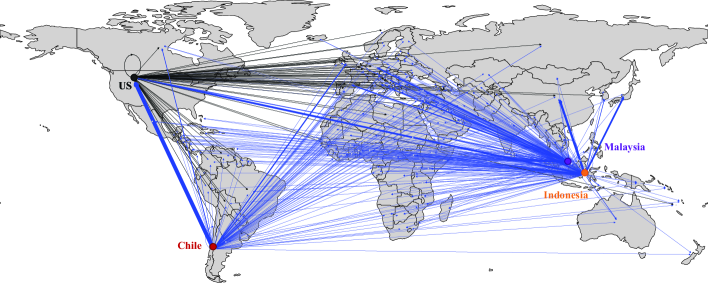
Figure 4: Back-shoring - selected countries and drug distribution under the base case conditions.

chicago supp-ref

References

- AAM (2021) AAM (2021). A blueprint for enhancing the security of the US pharmaceutical supply chain. Available at https://accessiblemeds.org/blueprint (accessed 2 May 2023).
- Aguiar and Kasper (2021) Aguiar, E. and E. Kasper (2021). Trade flows of parallel imported medicines in Europe. Available at https://affordablemedicines.eu/portfolio-item/position-paper-trade-flows-of-parallel-imported-medicines-2020/ (accessed 1 May 2023).
- Akbarpour et al. (2020) Akbarpour, M., S. Ali Torabi, and A. Ghavamifar (2020). Designing an integrated pharmaceutical relief chain network under demand uncertainty. Transportation Research Part E: Logistics and Transportation Review 136, 101867.
- Aldrighetti et al. (2021) Aldrighetti, R., D. Battini, D. Ivanov, and I. Zennaro (2021). Costs of resilience and disruptions in supply chain network design models: A review and future research directions. International Journal of Production Economics 235, 108103.
- Alevizakos et al. (2016) Alevizakos, M., M. Detsis, C. A. Grigoras, J. T. Machan, and E. Mylonakis (2016). The Impact of shortages on medication prices: Implications for shortage prevention. Drugs 76(16), 1551–1558.
- Ambulkar et al. (2015) Ambulkar, S., J. Blackhurst, and S. Grawe (2015). Firm’s resilience to supply chain disruptions: Scale development and empirical examination. Journal of Operations Management 33-34, 111–122.
- Barbieri et al. (2020) Barbieri, P., A. Boffelli, S. Elia, L. Fratocchi, M. Kalchschmidt, and D. Samson (2020). What can we learn about reshoring after Covid-19? Operations Management Research 13, 131–136.
- Blossey et al. (2021) Blossey, G., G. J. Hahn, and A. Koberstein (2021). Managing uncertainty in pharmaceutical supply chains: A structured review. In Proceedings of the Annual Hawaii International Conference on System Sciences, pp. 1435–1444.
- Blossey et al. (2022) Blossey, G., G. J. Hahn, and A. Koberstein (2022). Planning pharmaceutical manufacturing networks in the light of uncertain production approval times. International Journal of Production Economics 244(Oct 2021), 108343.
- Bochenek et al. (2018) Bochenek, T., V. Abilova, A. Alkan, …, and B. Godman (2018). Systemic measures and legislative and organizational frameworks aimed at preventing or mitigating drug shortages in 28 European and Western Asian countries. Frontiers in Pharmacology 8, 942.
- Casey and Cimino-Isaacs (2021) Casey, C. A. and C. D. Cimino-Isaacs (2021). Export restrictions in response to the COVID-19 pandemic. Available at https://crsreports.congress.gov/product/details?prodcode=IF11551 (accessed 2 May 2023).
- Chatzoglou et al. (2018) Chatzoglou, P., D. Chatzoudes, Z. Petrakopoulou, and E. Polychrou (2018). Plant location factors: A field research. Opsearch 55(3-4), 749–786.
- CIMA (2022) CIMA (2022). Shortage actives and supply problems. Available at https://cima.aemps.es/cima/publico/listadesabastecimiento.html (accessed 2 May 2023).
- Das (2018) Das, T. (2018). Managing Trust in Strategic Alliances. Research in Strategic Alliances. Charlotte, NC: Information Age Publishing Inc.
- Diaz et al. (2023) Diaz, R., S. Kolachana, and R. F. Gomes (2023). A simulation-based logistics assessment framework in global pharmaceutical supply chain networks. Journal of the Operational Research Society 74(5), 1242–1260.
- Duran et al. (2011) Duran, S., M. A. Gutierrez, and P. Keskinocak (2011). Pre-positioning of emergency items for CARE international. Interfaces 41(3), 223–237.
- Dyer (2019) Dyer, O. (2019). Us paediatric oncologists are forced to prioritise patients for vincristine treatment as supplies run short. BMJ 367, l6086.
- ECLAC (2021) ECLAC (2021). Plan for self-sufficiency in health matters in Latin America and the Caribbean: Lines of action and proposals. Available at https://hdl.handle.net/11362/47253 (accessed 5 May 2023).
- Franco and Alfonso-Lizarazo (2017) Franco, C. and E. Alfonso-Lizarazo (2017). A structured review of quantitative models of the pharmaceutical supply chain. Complexity 2017, 13.
- Ghavamifar et al. (2018) Ghavamifar, A., A. Makui, and A. A. Taleizadeh (2018). Designing a resilient competitive supply chain network under disruption risks: A real-world application. Transportation Research Part E: Logistics and Transportation Review 115(2018), 87–109.
- Goh et al. (2007) Goh, M., J. Y. Lim, and F. Meng (2007). A stochastic model for risk management in global supply chain networks. European Journal of Operational Research 182(1), 164–173.
- Goodarzian et al. (2020) Goodarzian, F., H. Hosseini-Nasab, J. Muñuzuri, and M. B. Fakhrzad (2020). A multi-objective pharmaceutical supply chain network based on a robust fuzzy model: A comparison of meta-heuristics. Applied Soft Computing Journal 92, 106331.
- Govindan et al. (2017) Govindan, K., M. Fattahi, and E. Keyvanshokooh (2017). Supply chain network design under uncertainty: A comprehensive review and future research directions. European Journal of Operational Research 263(1), 108–141.
- Hansen and Grunow (2015) Hansen, K. R. N. and M. Grunow (2015). Planning operations before market launch for balancing time-to-market and risks in pharmaceutical supply chains. International Journal of Production Economics 161, 129–139.
- Hasani and Khosrojerdi (2016) Hasani, A. and A. Khosrojerdi (2016). Robust global supply chain network design under disruption and uncertainty considering resilience strategies: A parallel memetic algorithm for a real-life case study. Transportation Research Part E: Logistics and Transportation Review 87, 20–52.
- Hilletofth et al. (2019) Hilletofth, P., D. Eriksson, W. Tate, and S. Kinkel (2019). Right-shoring: Making resilient offshoring and reshoring decisions. Journal of Purchasing and Supply Management 25(3).
- Iacocca et al. (2022) Iacocca, K., S. Mahar, and P. Daniel Wright (2022). Strategic horizontal integration for drug cost reduction in the pharmaceutical supply chain. Omega 108, 17.
- Jahre et al. (2016) Jahre, M., J. Kembro, T. Rezvanian, O. Ergun, S. J. Håpnes, and P. Berling (2016). Integrating supply chains for emergencies and ongoing operations in UNHCR. Journal of Operations Management 45, 57–72.
- Kalish and Wolf (2021) Kalish, I. and M. Wolf (2021). Supply chain resilience in the face of geopolitical risks. Available at https://www2.deloitte.com/us/en/insights/economy/us-china-trade-war-supply-chain.html (accessed 5 May 2023).
- Kchaou Boujelben and Boulaksil (2018) Kchaou Boujelben, M. and Y. Boulaksil (2018). Modeling international facility location under uncertainty: A review, analysis, and insights. IISE Transactions 50(6), 535–551.
- Kleywegt et al. (2002) Kleywegt, A. J., A. Shapiro, and T. Homem-de Mello (2002). The Sample Average Approximation Method for stochastic discrete optimization. SIAM Journal on Optimization 12(2), 479–502.
- Kochan and Nowicki (2018) Kochan, C. G. and D. R. Nowicki (2018). Supply chain resilience: A systematic literature review and typological framework. International Journal of Physical Distribution and Logistics Management 48(8), 842–865.
- Li et al. (2023) Li, J., Y. Liu, and G. Yang (2023). Two-stage distributionally robust optimization model for a pharmaceutical cold supply chain network design problem. International Transactions in Operational Research 0(0), 1–35.
- Li et al. (2020) Li, X., H. Wang, G. Hao, and C. Xia (2020). The mechanism of alliance promotes cooperation in the spatial multi-games. Physics Letters A 384(20), 126414.
- Li et al. (2023) Li, Z., T. Xia, W. Shen, and S. Chen (2023). Research on co-opetition mechanism between pharmaceutical enterprises and third-party logistics in drug distribution of medical community. International Journal of Environmental Research and Public Health 20(1), 19.
- Maharjan and Kato (2022) Maharjan, R. and H. Kato (2022). Resilient supply chain network design: A systematic literature review. Transport Reviews 42(6), 739–761.
- Marques et al. (2020) Marques, C. M., S. Moniz, J. P. de Sousa, A. P. Barbosa-Povoa, and G. Reklaitis (2020). Decision-support challenges in the chemical-pharmaceutical industry: Findings and future research directions. Computers and Chemical Engineering 134, 106672.
- Martei et al. (2020) Martei, Y. M., K. Iwamoto, R. D. Barr, J. T. Wiernkowski, and J. Robertson (2020). Shortages and price variability of essential cytotoxic medicines for treating children with cancers. BMJ Global Health 5(11), e003282.
- McIvor and Bals (2021) McIvor, R. and L. Bals (2021). A multi-theory framework for understanding the reshoring decision. International Business Review 30(6), 101827.
- McKinsey Global Institute (2020) McKinsey Global Institute (2020). Risk, resilience, and rebalancing in global value chains. Available at https://www.mckinsey.com/capabilities/operations/our-insights/risk-resilience-and-rebalancing-in-global-value-chains (accessed 2 May 2023).
- Mohiuddin et al. (2019) Mohiuddin, M., M. Rashid, S. A. Azad, and Z. Su (2019). Back-shoring or re-shoring: Determinants of manufacturing offshoring from emerging to least developing countries. International Journal Of Logistics: Research And Applications 22(1), 78–97.
- Namdar et al. (2018) Namdar, J., X. Li, R. Sawhney, and N. Pradhan (2018). Supply chain resilience for single and multiple sourcing in the presence of disruption risks. International Journal of Production Research 56(6), 2339–2360.
- NASEM (2022) NASEM (2022). Building Resilience into the Nation’s Medical Product Supply Chains. Washington, DC: The National Academies Press.
- Nguyen et al. (2021) Nguyen, H., T. C. Sharkey, S. Wheeler, J. E. Mitchell, and W. A. Wallace (2021). Towards the development of quantitative resilience indices for multi-echelon assembly supply chains. Omega 99, 102199.
- Ouazine et al. (2018) Ouazine, K., H. Slimani, and A. Tari (2018). Alliances in graphs: Parameters, properties and applications—A survey. AKCE International Journal of Graphs and Combinatorics 15(2), 115–154.
- Rawls and Turnquist (2010) Rawls, C. G. and M. A. Turnquist (2010). Pre-positioning of emergency supplies for disaster response. Transportation Research Part B: Methodological 44(4), 521–534.
- Sabogal De La Pava and Tucker (2022) Sabogal De La Pava, M. L. and E. L. Tucker (2022). Drug shortages in low- and middle-income countries: Colombia as a case study. Journal of Pharmaceutical Policy and Practice 15(1), 1–8.
- Sabouhi et al. (2018) Sabouhi, F., M. S. Pishvaee, and M. S. Jabalameli (2018). Resilient supply chain design under operational and disruption risks considering quantity discount: A case study of pharmaceutical supply chain. Computers and Industrial Engineering 126, 657–672.
- Santoso et al. (2005) Santoso, T., S. Ahmed, M. Goetschalckx, and A. Shapiro (2005). A stochastic programming approach for supply chain network design under uncertainty. European Journal of Operational Research 167(1), 96–115.
- Simon (2022) Simon, D. W. (2022). Managing supply chain disruption in an era of geopolitical risk. Available at https://www.foley.com/en/insights/publications/2022/07/avoid-supply-chain-disruption-geopolitical-risk (accessed 2 May 2023).
- Singh et al. (2019) Singh, C. S., G. Soni, and G. K. Badhotiya (2019). Performance indicators for supply chain resilience: Review and conceptual framework. Journal of Industrial Engineering International 15, 105–117.
- Singh et al. (2018) Singh, H., R. K. Garg, and A. Sachdeva (2018). Supply chain collaboration: A state-of-the-art literature review. Uncertain Supply Chain Management 6, 149–180.
- Snyder et al. (2016) Snyder, L. V., Z. Atan, P. Peng, Y. Rong, A. J. Schmitt, and B. Sinsoysal (2016). OR/MS models for supply chain disruptions: A review. IIE Transactions 48(2), 89–109.
- Sousa et al. (2011) Sousa, R. T., S. Liu, L. G. Papageorgiou, and N. Shah (2011). Global supply chain planning for pharmaceuticals. Chemical Engineering Research and Design 89(11), 2396–2409.
- Suda et al. (2022) Suda, K. J., K. C. Kim, I. Hernandez, W. F. Gellad, S. Rothenberger, A. Campbell, L. Malliart, and M. Tadrous (2022). The global impact of COVID-19 on drug purchases: A cross-sectional time series analysis. Journal of the American Pharmacists Association 62(3), 766–774.
- Suryawanshi and Dutta (2022) Suryawanshi, P. and P. Dutta (2022). Optimization models for supply chains under risk, uncertainty, and resilience: A state-of-the-art review and future research directions. Transportation Research Part E: Logistics and Transportation Review 157(Dec 2021), 1–45.
- Susarla and Karimi (2012) Susarla, N. and I. A. Karimi (2012). Integrated supply chain planning for multinational pharmaceutical enterprises. Computers and Chemical Engineering 42, 168–177.
- Tatar et al. (2022) Tatar, M., J. M. Shoorekchali, M. R. Faraji, M. A. Seyyedkolaee, J. A. Pagán, and F. A. Wilson (2022). COVID-19 vaccine inequality: A global perspective. Journal of Global Health 12, 10–13.
- The White House (2021) The White House (2021). Building Resilient Supply Chains, Revitalizing American Manufacturing, and Fostering Broad-Based Growth: 100-Day Reviews Under Executive Order 14017. Washington, DC: The White House.
- Tordecilla et al. (2021) Tordecilla, R. D., A. A. Juan, J. R. Montoya-Torres, C. L. Quintero-Araujo, and J. Panadero (2021). Simulation-optimization methods for designing and assessing resilient supply chain networks under uncertainty scenarios: A review. Simulation Modelling Practice and Theory 106(Aug 2020), 102166.
- Tucker and Daskin (2022) Tucker, E. L. and M. S. Daskin (2022). Pharmaceutical supply chain reliability and effects on drug shortages. Computers and Industrial Engineering 169, 108258.
- Tucker et al. (2020) Tucker, E. L., M. S. Daskin, B. V. Sweet, and W. J. Hopp (2020). Incentivizing resilient supply chain design to prevent drug shortages: Policy analysis using two- and multi-stage stochastic programs. IISE Transactions 52(4), 394–412.
- USTR (2022) USTR (2022). Free Trade Agreements. Available at https://ustr.gov/trade-agreements/free-trade-agreements (accessed 5 May 2023).
- UUDIS (2022) UUDIS (2022). Current Drug Shortages. Available at https://www.ashp.org/drug-shortages/current-shortages (accessed 3 May 2023).
- Varadarajan and Cunningham (1995) Varadarajan, P. R. and M. H. Cunningham (1995). Strategic alliances: A synthesis of conceptual foundations. Journal of the Academy of Marketing Science 23, 282–296.
- Verweij et al. (2003) Verweij, B., S. Ahmed, A. J. Kleywegt, G. Nemhauser, and A. Shapiro (2003). The Sample Average Approximation Method applied to stochastic routing problems: A computational study. Computational Optimization and Applications 24(2-3), 289–333.
- WTO (2020) WTO (2020). Export prohibitions and restrictions. Available at https://doi.org/10.30875/827540bd-en (accessed 5 May 2023).
- WTO (2022) WTO (2022). Trade monitoring database. Available at https://tmdb.wto.org/en/explore/goods\#nogo\%0A (accessed 1 October 2022).
- Zandkarimkhani et al. (2020) Zandkarimkhani, S., H. Mina, M. Biuki, and K. Govindan (2020). A chance constrained fuzzy goal programming approach for perishable pharmaceutical supply chain network design. Annals of Operations Research 295(1), 425–452.