A fast algorithm for All-Pairs-Shortest-Paths suitable for neural networks

Abstract

Given a directed graph of nodes and edges connecting them, a common problem is to find the shortest path between any two nodes. Here I show that the shortest path distances can be found by a simple matrix inversion: If the edges are given by the adjacency matrix $A_{ij}$ then with a suitably small value of $\gamma$ the shortest path distances are

$$D_{ij}=\operatorname{ceil}\left({\frac{\log{\left[{\left({\mathbf{1}}-\gamma{\mathbf{A}}\right)^{-1}}\right]}_{ij}}{\log\gamma}}\right)$$

I derive some bounds on $\gamma$ useful for a practical application. Even when the distance function is not globally accurate across the entire graph, it still works locally to instruct pursuit of the shortest path. In this mode, it also extends to weighted graphs with positive edge weights. For a wide range of dense graphs this distance function is computationally faster than the best available alternative. Finally I show that this method leads naturally to a neural network solution of the all-pairs-shortest-path problem.

1 Introduction

Many problems in animal behavior or in robotic control can be reduced to search on a graph. The graph may represent a spatial environment, like a road map, or a network of choices to be made in a cognitive task, like a game. Finding the shortest path from an initial state on the graph to a goal state is a central problem of graph theory [zwickExactAndApproximate2001, lewisAlgorithmsFindingShortest2020]. Generally an “all pairs shortest path” (APSP) algorithm delivers a matrix containing the distance for all pairs of nodes on the graph. That matrix can then be used iteratively to construct the actual sequence of nodes corresponding to the shortest path. Much mathematical effort has focused on efficient ways to compute the distance matrix.

In the most general formulation, an edge on the graph from point $j$ to node $i$ has a weight $W_{ij}$. The length of a path is the sum of the weight of its edges. The task is to find the shortest path between all pairs of points. Algorithms are evaluated – among other criteria – by their time complexity, namely how the number of basic operations depends on the number of vertices $V$ and number of edges $E$.

Graphs can be categorized by the constraints imposed on their edge weights:

• Undirected graphs have symmetric edge weights $W_{ij}=W_{ji}$. Directed graphs don’t have that constraint.

• Positive weights $W_{ij}>0$. If there are negative weights one generally requires that there be no cycles with negative distance.

• Integer weights. $W_{ij}\in\mathbb{N}$.

• Unweighted. $W_{ij}\in\{1,\infty\}$. In this case it only matters whether you can step from node $j$ to $i$ ($W_{ij}=1$) or not ($W_{ij}=\infty)$.

The Floyd-Warshall algorithm [floydAlgorithm97Shortest1962] is simple, works in all cases, and has time complexity $\mathcal{O}(V^{3})$. For undirected and unweighted graphs the Seidel algorithm [seidelAllPairsShortestPathProblemUnweighted1995] runs in $\mathcal{O}(V^{\omega}\log V)$ where $\omega$ is the complexity exponent for matrix multiplication, currently $\omega=2.373$. For directed but sparse graphs ($E\approx V$), there are various efficient methods, for example Johnson’s algorithm runs in $\mathcal{O}(EV+V^{2}\log V)$. However, for the general case of directed and dense ($E\approx V^{2}$) graphs there is currently no “sub-cubic” algorithm [chanMoreAlgorithmsAllPairs2010] that runs faster than $\mathcal{O}(EV)$.

Here I report that one gets a useful estimate of graph distances from the distance function

$$R_{ij}(\gamma)={\frac{\log{\left[{\left({\mathbf{1}}-\gamma^{\mathbf{W}}\right)^{-1}}\right]}_{ij}}{\log\gamma}}$$ (1)

using some suitably small value of $\gamma$. It was shown previously [chebotarevWalkDistancesGraphs2012] that as $\gamma$ approaches zero, $R_{ij}(\gamma)$ approaches the shortest path distances $D_{ij}$,

$$R_{ij}(\gamma)\xrightarrow[\gamma\rightarrow 0]{}D_{ij}$$ (2)

Here we will explore the behavior of the distance function at finite $\gamma$. We will see that the distance function of Eqn 1 offers a simple and practical solution to APSP over a wide range of graphs. On some computers at least, the computation proceeds faster than the conventional APSP algorithms. Finally, we will see that the algorithm is ideally suited for analog computing on a neural network architecture, including that of biological brains.

2 Derivations

First, I will derive the claim presented in the abstract. A proof for undirected graphs in the limiting case $\gamma\rightarrow 0$ can be found in [chebotarevWalkDistancesGraphs2012]. The present derivation extends to directed graphs and gives more insight as to what happens at finite $\gamma$.

2.1 Unweighted directed graph

Start with an unweighted directed graph defined by the adjacency matrix

$${A_{ij}}=\left\{{\begin{array}[]{*{20}{l}}{1,{\text{if you can take one step from node }}{j}{\text{ to node }}{i}}\\ {0,{\text{otherwise}}}\end{array}}\right.$$ (3)

It is well-known that the powers of the adjacency matrix represent the effects of multiple steps on the graph [biggsAlgebraicGraphTheory1993]:

$${\left[{{{\mathbf{A}}^{k}}}\right]_{ij}}=N_{ij}^{(k)}={\text{number of distinct paths to get from }}{j}{\text{ to }}{i}{\text{ in }}k{\text{ steps }}$$

Now choose a small $\gamma<<1$ and consider

$${\mathbf{Y}}(\gamma) =\left({\mathbf{1}}-\gamma{\mathbf{A}}\right)^{-1}$$ (4)

$$={\mathbf{1}}+\gamma{\mathbf{A}}+\gamma^{2}{\mathbf{A}}^{2}+\dots$$ (5)

Then

$$Y_{ij}(\gamma)=\sum_{k}N_{ij}^{(k)}\gamma^{k}$$ (6)

The shortest distance from node $j$ to node $i$ is the smallest $k$ with a non-zero path count $N_{ij}^{(k)}$:

$$D_{ij}=k_{\text{min}}=\min_{k}\left(N_{ij}^{(k)}>0\right)$$

Now suppose that $\gamma$ is chosen small enough that

$$\gamma<\frac{1}{N_{ij}^{(k)}}\text{ for all }i,j,k$$ (7)

Then we are guaranteed that

$$\gamma^{k_{\text{min}}}<Y_{ij}(\gamma)<\gamma^{{k_{\text{min}}}-1}$$ (8)

Now define a distance function

$$R_{ij}(\gamma)=\frac{\log Y_{ij}(\gamma)}{\log\gamma}=\frac{\log{\left[{\left({\mathbf{1}}-\gamma{\mathbf{A}}\right)^{-1}}\right]}_{ij}}{\log\gamma}$$ (9)

It follows from Eqn 8 that rounding up $R_{ij}$ produces the shortest graph distance:

$$\left\lceil R_{ij}(\gamma)\right\rceil=D_{ij}$$ (10)

where the brackets mean “round up to the nearest integer”.

Note that $R_{ij}(\gamma)$ is closely related to the resolvent function, defined as ${\left(\frac{1}{\gamma}{\mathbf{1}}-{\mathbf{A}}\right)^{-1}}$. Therefore I will call $R_{ij}(\gamma)$ the R-distance.

2.2 Integer weights

This result extends easily to the more general case of directed graphs with positive integer weights. Say the edge from node $j$ to node $i$ has weight $W_{ij}$ with

$$W_{ij}\in\mathbb{N}$$

The length of a path is defined as the sum of the weights of the edges. The distance $D_{ij}$ from $j$ to $i$ is the shortest length of a path from $j$ to $i$.

Note in the special case of an unweighted graph considered above, ${W_{ij}}=1$ for connected nodes and ${W_{ij}}=\infty$ otherwise.

Now define

$${\mathbf{X}}=\gamma^{\mathbf{W}}$$

meaning

$$X_{ij}=\gamma^{W_{ij}}$$

and

$${\mathbf{Y}(\gamma)} =\left({\mathbf{1}}-{\mathbf{X}}\right)^{-1}$$

$$={\mathbf{1}}+{\mathbf{X}}+{\mathbf{X}}^{2}+\dots$$

Note in the special case of an unweighted graph, ${\mathbf{X}}=\gamma{\mathbf{A}}$ is directly proportional to the adjacency matrix. As in the unweighted case, the powers of ${\mathbf{X}}$ represent the outcome of multi-step paths, but with an added dimension:

$${\left[{{{\mathbf{X}}^{k}}}\right]_{ij}}=\sum_{d}M_{ij}^{(k,d)}\gamma^{d}$$

where

$$M_{ij}^{(k,d)}={\text{number of distinct paths to get from }}{j}{\text{ to }}{i}{\text{ in }}k{\text{ steps with total length }}d$$

So the sum over those powers becomes

$$Y_{ij}(\gamma)=\sum_{d}N_{ij}^{(d)}\gamma^{d}$$ (11)

where

$$N_{ij}^{(d)}={\text{number of distinct paths to get from }}{j}{\text{ to }}{i}{\text{ with length }}d$$

Note the analogy to (6) above. So if one chooses $\gamma$ such that

$$\gamma<\frac{1}{N_{ij}^{(d)}}\text{ for all }i,j,d$$ (12)

then the R-distance function

$$R_{ij}(\gamma)={\frac{\log Y_{ij}(\gamma)}{\log\gamma}}={\frac{\log{\left[{\left({\mathbf{1}}-\gamma^{\mathbf{W}}\right)^{-1}}\right]}_{ij}}{\log\gamma}}$$ (13)

reports the shortest graph distances

$$\left\lceil R_{ij}(\gamma)\right\rceil=D_{ij}$$ (14)

2.3 Positive weights

Suppose the weights are positive but not restricted to integers. In the general case, every path will have a different weight, and the discretization that led to Eqns 9 and 13 does not apply. Instead, Eqn (6) becomes

$$Y_{ij}(\gamma)=\sum_{d\in\mathcal{D}}\gamma^{d}$$ (15)

where $\mathcal{D}$ is the set of all path weights. In the limit of small $\gamma$, the shortest distance $d_{\rm{min}}$ will dominate

$$Y_{ij}(\gamma)=\gamma^{d_{\rm{min}}}\left(1+\sum_{d>d_{\rm{min}}}\gamma^{(d-d_{\rm{min}})}\right)\xrightarrow[\gamma\rightarrow 0]{}\gamma^{d_{\rm{min}}}$$ (16)

So in the limit of small $\gamma$ the R-distance function

$$R_{ij}(\gamma)={\frac{\log Y_{ij}(\gamma)}{\log\gamma}}\xrightarrow[\gamma\rightarrow 0]{}D_{ij}$$ (17)

For finite $\gamma$ this R-distance function will not deliver the graph distance exactly, but may still be useful for finding the shortest path.

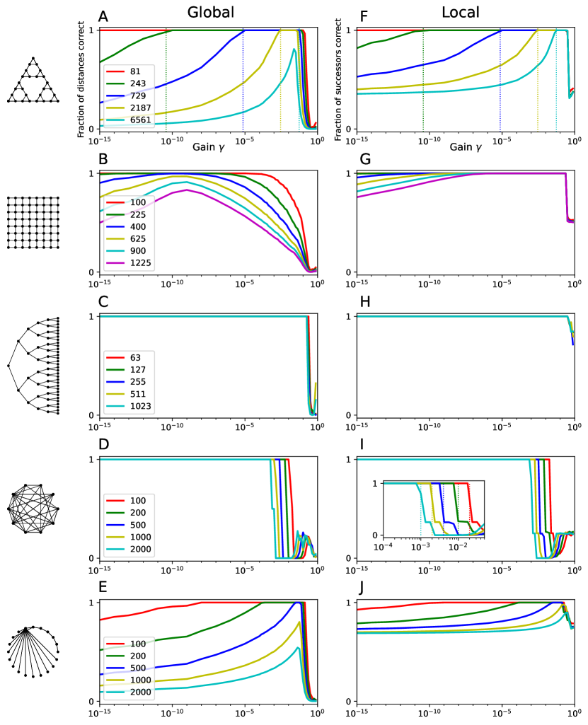
Figure 1: Performance of the R-distance. Each row represents a family of graphs illustrated by the icon on the left, with node numbers given in the legend. Global: Global performance: fraction of distances between nodes predicted correctly by Eqn 10, as a function of the gain parameter $\gamma$. Local: Local performance: fraction of successors predicted correctly according to Eqn 21. A: Global performance on graphs representing the Towers-of-Hanoi game. Dotted lines show the cutoff imposed by machine precision, according to Eqn 19. F: as in A, but for local performance. Note the valid range of $\gamma$ extends further to the right. B, G As in A and E, but for grid graphs: The nodes lie on a square Cartesian grid and each node connects to the 4 nearest neighbors. C, H Same, but for binary tree graphs, in which each node connects to 2 child nodes up to a certain number of levels. D, I Same, but for dense random graphs, in which each pair of nodes is connected with probability 0.5. I inset: Dotted lines indicate the critical gain, Eqn 18. E, J Same, but for graphs following a power law degree distribution (exponent = 3).

3 Performance of the R-distance

3.1 Global distance function

We begin by asking under what conditions the rounded R-distance function $\left\lceil R_{ij}(\gamma)\right\rceil$ produces the correct pairwise distances globally across the entire graph (Eqn 10). Figure 1A-E presents numerical results from various graph types, parametric in the number of nodes, illustrating the range of $\gamma$ that produces a globally correct R-distance. One can understand these behaviors based on the arguments in Section 2, which lead to several interesting bounds on the value of $\gamma$.

3.1.1 Critical gain

The Taylor expansion in Eqn 5 has a convergence radius of 1. So if the spectral radius of $\gamma{\bf{A}}$ exceeds 1, this expansion no longer holds, and thus ${\bf{Y}}(\gamma)$ no longer represents the lengths of paths on the graph (Eqn 6). Therefore an upper bound on $\gamma$ is given by the critical gain $\gamma_{\rm{c}}$,

$$\gamma<\gamma_{\rm{c}}\equiv\frac{1}{\lambda_{\rm{max}}}$$ (18)

where

$$\lambda_{\rm{max}}=\textrm{largest absolute eigenvalue of }{\bf{A}}$$

For unweighted graphs, the spectral radius is closely related to the number of edges per node [brouwerSpectraGraphs2012]. In Figure 1, the performance of the distance function has a sharp cut-off at large values of $\gamma$ for every graph type: this is the critical gain for that graph. For the random dense graphs (Fig 1D), the number of edges per node grows with the number of nodes, so the upper cutoff value of $\gamma$ decreases with the size of the graph.

3.1.2 Machine precision

Another constraint on $\gamma$ arises from the number representation in the computing system used. Suppose the largest distance on the graph is $d_{\rm{max}}$ and there is just one path with that distance. Then for that pair of nodes $Y_{ij}(\gamma)=\gamma^{d_{\rm{max}}}$ (Eqn 6). This must be a valid number, so it should exceed the smallest representable number $\delta$. This results in a lower bound for $\gamma$, namely

$$\gamma>\delta^{1/d_{\rm{max}}}$$ (19)

The effect of machine precision can be seen clearly for the Towers-of-Hanoi graphs, where the low-$\gamma$ cutoff is determined precisely by the longest distance on the graph (Fig 1A).

If a graph contains some long distances, then this lower bound may conflict with the upper bound given by the critical gain. To satisfy both, one requires

$$d_{\rm{max}}<\frac{\log\delta}{\log\gamma_{\rm{c}}}$$ (20)

For example, in double precision arithmetic (IEEE 754 standard) $\delta\approx 5\times 10^{-324}$. Suppose the graph has a spectral radius of $\lambda_{\rm{max}}\approx 10$, then $\gamma_{\rm{c}}\approx 0.1$, which sets a limit on the maximal distance $d_{\rm{max}}<323$. If the graph includes larger distances, then the R-distance function cannot be globally correct for any value of $\gamma$. One can see this conflict for the larger Tower-of-Hanoi graphs (Fig 1A) and in certain Power law graphs (Fig 1E).

3.1.3 Redundant paths

As discussed in section 2 (Eqn 7), $1/\gamma$ should exceed the number of redundant paths ${N_{ij}^{(k)}}$, namely the number of paths from node $j$ to $i$ that all have length $k$. Depending on the graph type, this number may be very large or very small. For example, on a binary tree, there is just one shortest path between any two nodes. By contrast, on a grid graph (nodes and edges following a square grid), there may be a huge number of such redundant paths. In that case, one finds that the constraint $\gamma<{N_{ij}^{(k)}}$ takes its toll, by greatly limiting the upper range of $\gamma$ (Fig 1B). However, this high degree of redundancy does not appear in the other graph types tested here (Fig 1A,C,D,E). The binary tree graphs allow the greatest range of $\gamma$ for a perfect R-distance, with the only practical constraint being the critical gain (Fig 1C). These trees don’t suffer from redundant paths, and the maximal distance grows only logarithmically with the number of nodes.

3.2 Local distance function

Perhaps the most common use of an all-pairs distance matrix $D_{ij}$ is to find the actual shortest paths between any two nodes on the graph. A simple greedy-descent algorithm accomplishes this. Say the goal node is $g$. Starting from node $i$, find all the nodes connected to it. Within that set of successor nodes ${\mathcal{S}}(i)$, choose the node $j$ that has the shortest distance $D_{gj}$ to the goal:

$$i\leftarrow\underset{j\in{\mathcal{S}}(i)}{\operatorname{argmin}}\,D_{gj}$$ (21)

Then iterate this step until the goal is reached.

If one uses the R-distance function $R_{gj}$ for this algorithm instead of the exact graph distances $D_{gj}$, one will of course find the shortest paths if the R-distance is globally accurate across the entire graph (Eqn 10, Fig 1A-E). However, the R-distance turns out to yield shortest paths even when it is not globally accurate. Over a wide range of $\gamma$, the R-distance, when applied in Eqn 21, chooses the correct successor node for all pairs of start and goal nodes (Fig 1F-J). In those cases one can say the R-distance is locally correct.

The effect is most pronounced for the example of grid graphs (Fig 1G). Here, a wide range of $\gamma$ supports locally correct performance, even when there exists no $\gamma$ that produces globally correct distances (Fig 1B). Among the three mathematical constraints on $\gamma$ identified in Section 3.1, the critical gain (Eqn 18) and the machine precision (Eqn 19) still apply. However, the constraint from redundant paths (Eqn 7) has fallen away. This is because the number of paths ${N_{gj}^{(k)}}$ with identical distance $k$ to the goal $g$ will be very similar among nearby nodes $j$ that are all neighbors of $i$. That number of redundant paths may vary enormously across the entire graph, but only little within a tight neighborhood. This is why making local comparisons of the R-distance among nearby points still identifies the node nearest the goal correctly.

For all the graphs tested in Figure 1 the R-distance is locally correct as long as $\gamma$ lies between the lower bound from machine precision and the upper bound of critical gain (Fig 1I inset). If one has an expectation for the critical gain $\gamma_{\rm{c}}$, then one can choose $\gamma$ just below that.

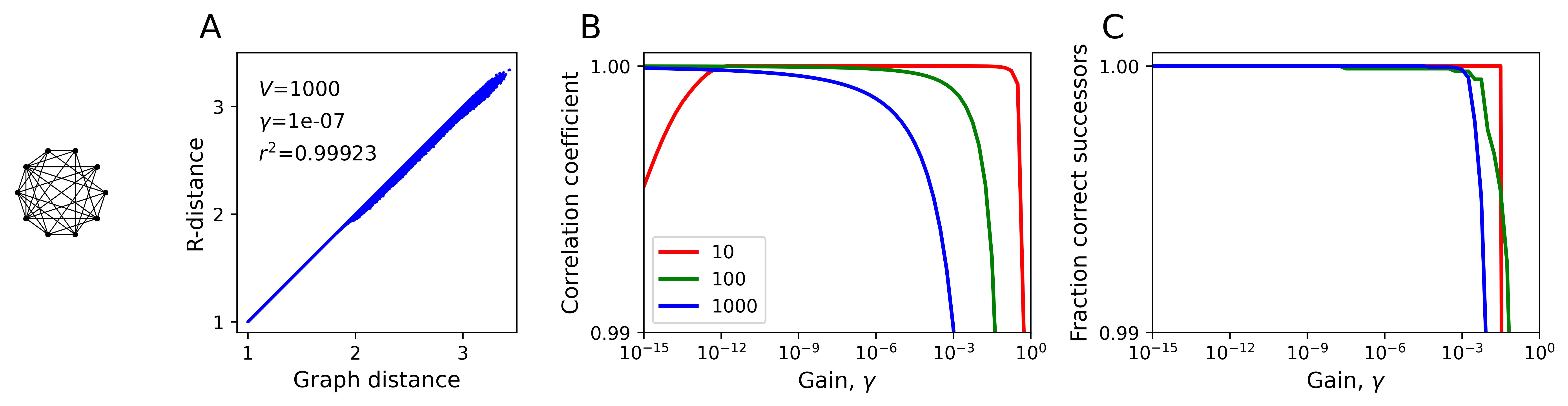
Figure 2: The R-distance on weighted graphs. Results on a dense graph (as in Fig 1D,I) with random positive edge weights. A: The R-distance plotted against the true graph distance. $V=1000$ vertices, $p=0.5$ edge probability, edge weights range from 1 to 100 with log-uniform distribution. $\gamma=10^{-7}$. Note high correlation coefficient $r^{2}$. B: Global performance. The correlation coefficient $r^{2}$ between R-distance and true graph distance, for graphs of various sizes ($V$ in legend) as a function of the gain $\gamma$. Note y-axis scale is close to 1. C: Local performance. The fraction of correct successors predicted by the R-distance. At $\gamma<10^{-8}$ all 1 million successors in the $V=1000$ graph are predicted correctly.

3.3 Real positive weights

So far, we have considered unweighted graphs where the edges are either present or not. However, as derived in Section 2, the R-distance should be a useful measure also on weighted graphs, as long as the edge weights are positive real numbers. On a weighted graph, the length of a path is the sum of the weights of its edges, and the shortest path is the one with the smallest total weight.

Figure 2 illustrates the relation of the R-distance to the true distance on a dense graph with random positive weights, whose values span two orders of magnitude. Because the distance can take on any real value, one cannot expect the R-distance to be exact. However, it can be tightly correlated to the real distance (Fig 2A), and over a wide range of gain values $\gamma$ the correlation is almost perfect (Fig 2B). Furthermore, over a wide range of $\gamma$, the R-distance is locally correct, in that it identifies every correct successor node for the shortest path (Fig 2C).

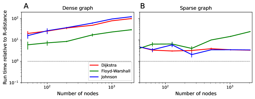
Figure 3: Run times to compute distance functions. The run times for 3 conventional APSP algorithms, compared to that for the R-distance. The algorithms are Floyd-Warshall, Dijkstra, and Johnson, as implemented in the Python package scipy. A: Dense graphs (random unweighted with edge probability 0.5) with varying node numbers. All run times are divided by that for the R-distance. Dotted line: equality. Mean over 25 runs, bars indicate standard error. B: As in (A) for sparse graphs (binary tree). Note for all these graphs the conventional APSP algorithms are slower than the R-distance.

4 Complexity and run times on digital computers

The time complexity of the R-distance (Eqn 9) is dominated by the matrix inversion, which for a graph with $V$ vertices has complexity $\mathcal{O}(V^{\omega})$ (currently $\omega=2.373$). This improves on published algorithms for APSP on dense directed graphs, which have a higher polynomial dependence on $V$ [zwickExactAndApproximate2001]. For example, Takaoka’s algorithm for graphs with integer weights [takaokaSubcubicCostAlgorithms1998] runs in $\mathcal{O}(M^{1/3}V^{(6+\omega)/3})$ where $M$ is the largest weight. Thus the R-distance proposed here has a time-complexity better than all known algorithms for dense directed graphs [chanMoreAlgorithmsAllPairs2010].

However, this theoretical advantage comes with some caveats. For one, the R-distance can be globally correct only if the critical gain exceeds the lower bound imposed by the machine precision and the longest distance (Eqn 20). As the number of vertices $V$ grows, the largest distance on the graph will grow as well, necessitating greater bit depth for the computation. As $V$ goes to infinity, one would need infinite machine precision. Effectively the computation of R-distance pushes part of the complexity from time into space. It shares that characteristic with some other APSP algorithms that presume infinite machine precision [yuvalAlgorithmFindingAll1976].

Second, from a practical perspective, there is no current implementation of matrix inversion or even matrix multiplication that runs in $\mathcal{O}(V^{\omega})$. Some have expressed doubts whether a machine will ever be built on which the Coppersmith-Winograd algorithm [coppersmithMatrixMultiplicationArithmetic1990] offers a benefit over the schoolbook $\mathcal{O}(V^{3})$ multiplication [robinsonOptimalAlgorithmMatrix2005]. Certainly the popular scientific programming platforms all invert dense matrices with an $\mathcal{O}(V^{3})$ algorithm.

Nonetheless, we have found in practice that the R-distance is locally correct on many graphs up to thousands of nodes in size (Figs 1, 2). Furthermore, in at least one popular scientific programming environment (Python scipy) its evaluation is more than $10\times$ faster than the Floyd-Warshall algorithm on dense graphs (Fig 3A). Even on sparse graphs, the R-distance is considerably faster than Dijkstra’s and Johnson’s algorithms, which were designed for sparse graphs (Fig 3B). This can be attributed to the extensive effort that has gone into optimizing the routines for matrix inversion. Possibly, a similar degree of scrutiny could be applied to optimizing the APSP algorithms beyond their current implementation in popular libraries.

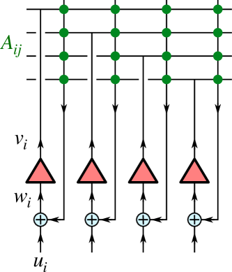
Figure 4: Analog circuit to compute R-distances Each of the linear units (triangles) receives input $w_{i}$ and generates output $v_{i}=\gamma w_{i}$. The input is combined from an external drive $u_{i}$ and feedback from the outputs through the connections $A_{ij}$.

5 Analog computation

Having found that the R-distance is broadly useful and efficient as a measure of graph distances (Figs 1, 2, 3) we come to another distinguishing trait: the R-distance is uniquely suited for analog computation.

Figure 4 shows a simple network of linear analog units with recurrent feedback. Each unit $i$ has an input $w_{i}$ that it converts to an output $v_{i}$,

$$v_{i}=\gamma\,w_{i}$$ (22)

where $\gamma$ is the gain of the units. The input consists of an external signal $u_{i}$ summed with a recurrent feedback through a connection matrix ${\bf{A}}$:

$$w_{i}=u_{i}+\sum_{ij}A_{ij}v_{j}$$ (23)

Combining Eqns 22 and 23, one finds the solution

$${\vec{v}}=\left(\frac{1}{\gamma}{\bf{1}}-{\bf{A}}\right)^{-1}{\vec{u}}$$ (24)

Note the correspondence to the expression for the R-distance (Eqn 9). Specifically, suppose that the input is set to zero, except at node $s$,

$$u_{i}=\begin{cases}1,&\text{if}\ i=s\\ 0,&\text{otherwise}\end{cases}$$ (25)

Then the network output $\vec{v}$ reflects the R-distances from $s$ to all the other nodes, namely:

$$v_{i}=\gamma^{1+R_{is}(\gamma)}$$ (26)

In other words, if one sets the connection matrix of the network in Fig 4 to the adjacency matrix $A_{ij}$ of a graph, then the network output will compute the R-distances $R_{is}$ on the graph from any desired starting node, chosen by setting its input $u_{s}$ to 1. Specifically, the output $v_{i}$ is a monotonically decreasing function of $R_{is}$.

One can envision computing all the pairwise distances by sequentially setting the input signals to 1 one at a time, and recording the results, thus accumulating the full APSP matrix $R_{ij}$. However, a more compelling application uses the network dynamically while finding the shortest path to a goal. Set the input of the starting node $s$ to 1. Measure the output of node $g$: this signal increases as $s$ gets closer to the goal. Try all the successor nodes of $s$ by setting their inputs to 1, and pick the one that produces the largest output. Then iterate until you reach the goal node. This essentially implements the procedure of Eqn 21 by computing the required columns of $R_{ij}$ one at a time on the way to the goal.

Note that this network requires only $\mathcal{O}(V)$ active units, where $V$ is the number of vertices of the graph in question. If implemented as an electronic circuit, each unit is a simple amplifier and can be built from a few transistors. The edges $A_{ij}$ of the graph may be stored in passive elements like resistors. One could even add a stage that performs the above selection during path-finding (Eqn 21) with a Winner-take-all circuit, again at a cost of just a few transistors per node [lazzaroWinnerTakeAllNetworksComplexity1988].

In summary, the R-distance function maps conveniently onto a simple network architecture for analog computing. This feature recommends the R-distance for implementation of graph search in electronic circuits, artificial neural networks, and real circuits of neurons in the brain.

6 Discussion

6.1 Related work

The central observation here is that one can obtain all the pairwise shortest distances on a graph directly from the resolvent function $\left({\bf{1}}-\gamma{\bf{A}}\right)^{-1}$ of its adjacency matrix (Section 2). The approach is valid over a wide range of graph types and sizes (Section 3) and performs efficiently compared to conventional APSP algorithms (Section 4). Unlike other known algorithms, computation of the R-distance maps naturally onto an analog neural network (Section 5).

The resolvent function has played a important role in the analysis of graphs for some time [katzNewStatusIndex1953, benziMatrixFunctionsNetwork2020], and the developments here may allow another interpretation of those measures. For example, the "resolvent-based total communicability" has been defined [benziTotalCommunicabilityCentrality2013] as

$$C_{r}({\bf{A}})=\sum_{i=1}^{n}\sum_{j=1}^{n}\left[\left({\bf{1}}-\gamma{\bf{A}}\right)^{-1}\right]_{ij}$$ (27)

The authors recommend setting $\gamma$ just below the critical value, $\gamma=0.85\,\gamma_{\rm{c}}$, without much justification. From Figure 1 we see that this value is too close to the critical value to produce a globally correct distance function on most graphs. Hence the meaning of this measure will depend strongly on the graph type. If we choose $\gamma$ somewhat smaller, say $\gamma=0.01\gamma_{\rm{c}}$, then we can use Eqn 9 to reinterpret the communicability. In that case, $C_{r}$ becomes a simple function of all the graph distances $D_{ij}$:

$$C_{r}=\sum_{i=1}^{n}\sum_{j=1}^{n}\gamma^{D_{ij}}$$ (28)

This gives a more concrete understanding of the concept of "communicability".

With the goal of determining all shortest paths, a recent report [steinerbergerSpectralApproachShortest2021] attempts a solution based on the Laplacian matrix, which is related to the resolvent, but lacks the degree of freedom given by $\gamma$. That method is computationally expensive, gives provably correct results only on trees, and fails even on elementary graphs [jourdanSpectralMethodFinding2021]. Another study used the resolvent function to estimate graph distances [baramIntuitivePlanningGlobal2018], but again with a fixed value of $\gamma=0.85\,\gamma_{\rm{c}}$, and found empirically that the estimates were approximately correct on some graphs. Again, the developments presented here explain why and how one should choose $\gamma$ to obtain a useful distance function.

6.2 Applications

On digital computers, the R-distance probably offers limited benefits over conventional APSP algorithms. While it does execute faster than the plain-vanilla implementations of APSP on graphs with several thousand nodes (Fig 3), any truly time-critical application will likely involve huge graphs. If the longest distance on the graph exceeds a few hundred nodes, the R-distance algorithm will run into the machine precision limit (Eqn 20). Furthermore, considerable effort is spent optimizing Floyd-Warshall for large node numbers and GPU architectures, achieving efficiencies similar to the high-performance routines for matrix inversion [saoScalableAllpairsShortest2021].

By contrast, the R-distance function seems perfectly adapted for analog computation. In the circuit of Figure 4, the knowledge of the graph is embodied in the feedback connection strengths, and the network output can be used to navigate on the graph. For example, one can envision such a circuit in a robot control system. Here the graph represents a map of the environment with navigable paths between nodes. The robot specifies the goal location, by measuring unit $g$’s output, and its current location, by setting unit $i$’s input to 1. Then it queries the analog network for the next step to take towards the goal (Eqn 21). Often a robot must navigate in an uncertain environment, and update its map when a new obstacle is encountered [koenigFastReplanningNavigation2005]. Then the shortest paths must be recomputed dynamically. For this purpose, the circuit of Figure 4 is “always on” and responds instantaneously to any changes in the connection strengths $A_{ij}$ or in the current input node. If implemented in analog electronics, the settling time for the new result could be microseconds or less. The low component count, with just a few transistors per node, may allow miniaturization of such a circuit down to millimeter-sized robots.

Another suitable analog network is the brain. Animal brains must routinely solve problems that reduce to search on a graph. Take the explicit instance of spatial navigation: An animal explores a new physical environment, learns the available paths between points, then navigates towards chosen goal locations on that graph [tolman1948cognitive]. These functions are essential to insects, with brains of $\sim 10^{5}$ neurons, as much as to humans with $\sim 10^{10}$ [webbNeuralMechanismsInsect2016, epsteinCognitiveMapHumans2017]. One suspects that evolution has found an efficient way to handle graph search using a neural network. Indeed, the circuit in Figure 4 is a common motif found in animal brains [dayan_theoretical_2001, muller_hippocampus_1996, douglasRecurrentNeuronalCircuits2007]. Here each active unit is a neuron or a group of neurons, and the connections are recurrent synapses among those neurons. Thus the R-distance computed by such a neural circuit could serve as the goal signal that guides the animal’s navigation. Of course several additional problems must be solved: how to learn the synaptic connections $A_{ij}$ during spatial exploration; how to learn about interesting locations on the map and store them for future navigation; how to maintain multiple maps of different environments. This is an area of intense investigation [sosaNavigatingReward2021, peerStructuringKnowledgeCognitive2021]. A recent report proposes and end-to-end solution that implements all these functions on the basis of the R-distance [zhangEndotaxisNeuromorphicAlgorithm2022].

Code availability

Code to produce the figures is available in a public repository: https://github.com/markusmeister/APSP.

References

References

- Zwick [2001] Uri Zwick. Exact and approximate distances in graphs — A survey. In Friedhelm Meyer auf der Heide, editor, Algorithms — ESA 2001, pages 33–48, Berlin, Heidelberg, 2001. Springer Berlin Heidelberg. ISBN 978-3-540-44676-7.
- Lewis [2020] Rhyd Lewis. Algorithms for Finding Shortest Paths in Networks with Vertex Transfer Penalties. Algorithms, 13(11):269, November 2020. ISSN 1999-4893. doi: 10.3390/a13110269.
- Floyd [1962] Robert W. Floyd. Algorithm 97: Shortest path. Communications of the ACM, 5(6):345, June 1962. ISSN 0001-0782. doi: 10.1145/367766.368168.
- Seidel [1995] R. Seidel. On the All-Pairs-Shortest-Path Problem in Unweighted Undirected Graphs. J. Comput. Syst. Sci., 1995. doi: 10.1006/jcss.1995.1078.
- Chan [2010] Timothy M. Chan. More Algorithms for All-Pairs Shortest Paths in Weighted Graphs. SIAM Journal on Computing, 39(5):2075–2089, January 2010. ISSN 0097-5397. doi: 10.1137/08071990X. URL https://epubs.siam.org/doi/10.1137/08071990X. Publisher: Society for Industrial and Applied Mathematics.
- Chebotarev [2012] Pavel Chebotarev. The walk distances in graphs. Discrete Applied Mathematics, 160(10):1484–1500, July 2012. ISSN 0166-218X. doi: 10.1016/j.dam.2012.02.015.
- Biggs [1993] Norman Linstead Biggs. Algebraic Graph Theory. Cambridge University Press, 1993. ISBN 978-0-521-45897-9.
- Brouwer and Haemers [2012] Andries E. Brouwer and Willem H. Haemers. Spectra of Graphs. Universitext. Springer, New York, NY, 2012. ISBN 978-1-4614-1938-9 978-1-4614-1939-6. doi: 10.1007/978-1-4614-1939-6.
- Takaoka [1998] T. Takaoka. Subcubic Cost Algorithms for the All Pairs Shortest Path Problem. Algorithmica, 20(3):309–318, March 1998. ISSN 1432-0541. doi: 10.1007/PL00009198.
- Yuval [1976] G. Yuval. An Algorithm for Finding All Shortest Paths Using Infinite-Precision Multiplications. Information Processing Letters, 4(6):155–156, March 1976. ISSN 0020-0190. doi: 10.1016/0020-0190(76)90085-5.
- Coppersmith and Winograd [1990] Don Coppersmith and Shmuel Winograd. Matrix multiplication via arithmetic progressions. Journal of Symbolic Computation, 9(3):251–280, March 1990. ISSN 0747-7171. doi: 10.1016/S0747-7171(08)80013-2.
- Robinson [2005] Sara Robinson. Toward an Optimal Algorithm for Matrix Multiplication. SIAM News, 38(9), November 2005.
- Lazzaro et al. [1988] J. Lazzaro, S. Ryckebusch, M.A. Mahowald, and C. A. Mead. Winner-Take-All Networks of O(N) Complexity. In Advances in Neural Information Processing Systems, volume 1. Morgan-Kaufmann, 1988.
- Katz [1953] Leo Katz. A new status index derived from sociometric analysis. Psychometrika, 18(1):39–43, March 1953. ISSN 1860-0980. doi: 10.1007/BF02289026.
- Benzi and Boito [2020] Michele Benzi and Paola Boito. Matrix functions in network analysis. GAMM-Mitteilungen, 43(3):e202000012, 2020. ISSN 1522-2608. doi: 10.1002/gamm.202000012.
- Benzi and Klymko [2013] Michele Benzi and Christine Klymko. Total communicability as a centrality measure. Journal of Complex Networks, 1(2):124–149, December 2013. ISSN 2051-1310. doi: 10.1093/comnet/cnt007.
- Steinerberger [2021] Stefan Steinerberger. A spectral approach to the shortest path problem. Linear Algebra and its Applications, 620:182–200, July 2021. ISSN 0024-3795. doi: 10.1016/j.laa.2021.02.013.
- Jourdan [2021] Ben Jourdan. On the Spectral Method for Finding Shortest Paths: A Characterisation and Counterexample. Master of Science, The University of Edinburgh, Edinburgh, UK, 2021.
- Baram et al. [2018] Alon B. Baram, Timothy H. Muller, James C. R. Whittington, and Timothy E. J. Behrens. Intuitive planning: Global navigation through cognitive maps based on grid-like codes, September 2018.
- Sao et al. [2021] Piyush Sao, Hao Lu, Ramakrishnan Kannan, Vijay Thakkar, Richard Vuduc, and Thomas Potok. Scalable All-pairs Shortest Paths for Huge Graphs on Multi-GPU Clusters. In Proceedings of the 30th International Symposium on High-Performance Parallel and Distributed Computing, HPDC ’21, pages 121–131, New York, NY, USA, June 2021. Association for Computing Machinery. ISBN 978-1-4503-8217-5. doi: 10.1145/3431379.3460651.
- Koenig and Likhachev [2005] S. Koenig and M. Likhachev. Fast replanning for navigation in unknown terrain. IEEE Transactions on Robotics, 21(3):354–363, June 2005. ISSN 1552-3098. doi: 10.1109/TRO.2004.838026.
- Tolman [1948] E. C. Tolman. Cognitive maps in rats and men. Psychological Review, 55(4):189–208, 1948. ISSN 0033-295X. doi: 10.1037/h0061626.
- Webb and Wystrach [2016] Barbara Webb and Antoine Wystrach. Neural mechanisms of insect navigation. Current Opinion in Insect Science, 15:27–39, June 2016. ISSN 2214-5745. doi: 10.1016/j.cois.2016.02.011.
- Epstein et al. [2017] Russell A. Epstein, Eva Zita Patai, Joshua B. Julian, and Hugo J. Spiers. The cognitive map in humans: Spatial navigation and beyond. Nature Neuroscience, 20(11):1504–1513, November 2017. ISSN 1546-1726. doi: 10.1038/nn.4656.
- Dayan and Abbott [2001] Peter Dayan and L. F. Abbott. Theoretical Neuroscience: Computational and Mathematical Modeling of Neural Systems. Computational Neuroscience. MIT Press, Cambridge, Mass., 2001.
- Muller et al. [1996] R. U. Muller, M. Stead, and J. Pach. The hippocampus as a cognitive graph. The Journal of General Physiology, 107(6):663–694, June 1996. ISSN 0022-1295. doi: 10.1085/jgp.107.6.663.
- Douglas and Martin [2007] Rodney J. Douglas and Kevan A. C. Martin. Recurrent neuronal circuits in the neocortex. Current biology: CB, 17(13):R496–500, July 2007. ISSN 0960-9822. doi: 10.1016/j.cub.2007.04.024.
- Sosa and Giocomo [2021] Marielena Sosa and Lisa M. Giocomo. Navigating for reward. Nature Reviews Neuroscience, pages 1–16, July 2021. ISSN 1471-0048. doi: 10.1038/s41583-021-00479-z.
- Peer et al. [2021] Michael Peer, Iva K. Brunec, Nora S. Newcombe, and Russell A. Epstein. Structuring Knowledge with Cognitive Maps and Cognitive Graphs. Trends in Cognitive Sciences, 25(1):37–54, January 2021. ISSN 1364-6613. doi: 10.1016/j.tics.2020.10.004.
- Zhang et al. [2022] Tony Zhang, Matthew Rosenberg, Pietro Perona, and Markus Meister. Endotaxis: A neuromorphic algorithm for mapping, goal-learning, navigation, and patrolling. bioRxiv, page 2021.09.24.461751, October 2022. doi: 10.1101/2021.09.24.461751.