PARIS: Part-level Reconstruction and Motion Analysis for Articulated Objects

Abstract

We address the task of simultaneous part-level reconstruction and motion parameter estimation for articulated objects. Given two sets of multi-view images of an object in two static articulation states, we decouple the movable part from the static part and reconstruct shape and appearance while predicting the motion parameters. To tackle this problem, we present PARIS: a self-supervised, end-to-end architecture that learns part-level implicit shape and appearance models and optimizes motion parameters jointly without any 3D supervision, motion, or semantic annotation. Our experiments show that our method generalizes better across object categories, and outperforms baselines and prior work that are given 3D point clouds as input. Our approach improves reconstruction relative to state-of-the-art baselines with a Chamfer-L1 distance reduction of $3.94$ ($45.2\%$) for objects and $26.79$ ($84.5\%$) for parts, and achieves 5% error rate for motion estimation across 10 object categories.

1 Introduction

Articulated objects consist of interconnected static and movable parts that exhibit motion. Such objects are ubiquitous in real life (e.g., drawers, ovens, chairs, laptops, staplers). Thus, perception and understanding of articulated object structure is important in many areas including robotics [49, 25, 9, 23], animation [39, 7], and industrial design [19]. Articulated object motion analysis enables robots to manipulate objects more effectively [11]. Acquiring digital replicas of articulated objects [20, 16] also enables simulating object articulation in applications involving robotic agents and embodied AI [37, 41].

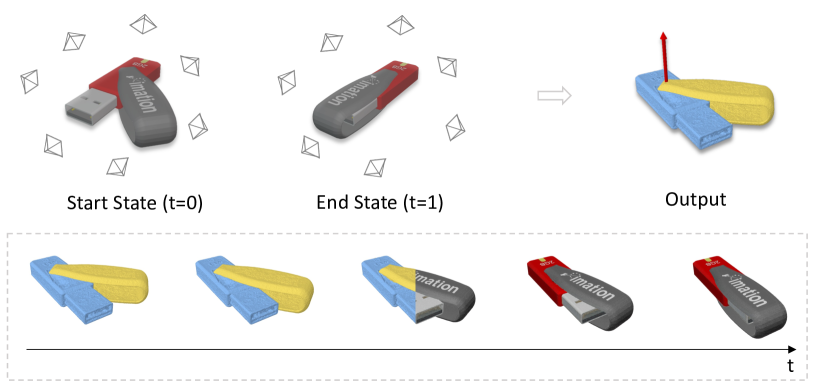
Figure 1: We present PARIS: a method that takes only multi-view images of an object in two articulation states (top left) and recovers part-level shape and appearance while jointly estimating articulation motion parameters (top right). Our method can generate unseen states and render the object from arbitrary views (bottom).

Prior work on articulated object understanding uses supervised learning which requires 3D supervision and articulation annotation [45, 50]. Unfortunately, such supervisory data is expensive and unavailable at scale. Another line of prior work assumes a known object category and learns separate models for each category [21, 29, 47, 43]. This makes generalization to arbitrary unseen objects difficult. Recently, Jiang et al. [20] proposed Ditto: a category-agnostic approach for motion and part geometry prediction from a pair of 3D point clouds. However, this approach is limited in generalization to unseen object categories and it does not address detailed appearance reconstruction.

We make the observation that perception of articulated objects involves two subproblems: reconstruction and motion analysis. These subproblems are tightly intertwined since knowing the complete geometry of an object makes motion analysis easier, while knowing the motion parameters of an object provides a signal for better reconstruction of the object given observations in different articulation states. Our insight is that by leveraging the intertwined nature of articulated object perception we can avoid reliance on explicit 3D data and motion parameter supervision.

In this paper, we propose PARIS: a self-supervised approach for joint reconstruction and motion analysis of articulated objects. By observing an articulated object in two states (see Figure 1), our method reconstructs the shape and appearance of the static and movable parts in two implicit neural fields, while predicting the articulation motion parameters. The separated neural fields are composited using the estimated motion parameters to set up self-supervisory losses relying only on the input RGB images.

Thus, our approach is category-agnostic and does not require any 3D data or supervisory signals for part segmentation, motion parameters, or object category semantics.

In summary:

• We address joint reconstruction and motion analysis for articulated objects including part-level shape and appearance, and motion estimation given RGB images of the object in only two static states.

• We develop PARIS: a category-agnostic, self-supervised and end-to-end approach that jointly performs reconstruction and motion analysis without 3D supervision, motion parameter or semantic annotation.

• We systematically evaluate our approach on synthetic and real data, and show we significantly outperform prior work and baselines in shape and appearance quality, and motion parameter estimation accuracy.

2 Related Work

Movable part segmentation and analysis. The analysis of part mobility is a well-established challenge for understanding the kinematics of articulated objects [1, 28, 14, 11]. With more 3D data and annotations of articulation being collected for articulated objects, recent works favor tackling this problem from 3D inputs in a data-driven fashion. ScrewNet [18] uses a recurrent neural network to predict articulation without part segmentation, from a sequence of depth images. Assuming part segmentation is given, Hu et al. [17] estimate the part mobilities by mapping a point cloud to a class of motion sequences via metric learning.

Although many approaches have been proposed to conduct semantic segmentation on 3D shapes [35, 52], the obtained part segmentation does not necessarily conform to mobilities. Considering this obstacle, later works address the mobility part segmentation and analysis collectively. Taking a single point cloud as input, Shape2Motion [45] and Li et al. [21] propose to learn a category-level model to address this coupled task in a supervised way. These models have only limited generalization to arbitrary unseen objects since a separate trained model is required for each category. To mitigate dependency on the object category, Yan et al. [50] and Abdul-Rashid et al. [2] design cross-category networks to predict part segmentation and kinematic hierarchy from a point cloud. Liu et al. [22] learn part motion parameters from an over-segmented 3D scan in a semi-supervised manner. Chu et al. [5] proposes a category-agnostic method to manipulate the articulated parts to predefined states driven by a user command.

The above works all focus on understanding the articulation and 3D structure of a point cloud. Our work reconstructs part-level surface and appearance jointly with motion estimation from only RGB images, which are more readily available compared to 3D or depth inputs. The closest work is Ditto [20] which also produces part-level surface and articulation parameters by observing two states of the object as the input. Another similar concurrent work is CARTO [15] which reconstructs object surfaces with motion estimated from stereo images. The main differences are the following: 1) Ditto takes a pair of 3D point clouds as input, while we use two sets of multi-view RGB images of the object in two states; 2) Ditto and CARTO only produce geometry (no texture or other surface appearance) and CARTO cannot reconstruct parts; 3) The work mentioned above requires 3D supervision and articulation annotation during training, while our approach is self-supervised only with images.

Implicit models for articulated objects. Neural implicit models are increasingly popular because of their continuous and topology-free representation. In early works, shape and deformation modeling of articulated objects with implicit functions requires 3D supervision e.g., NASA [8] for human objects and A-SDF [29] for general articulated objects. With the success of differentiable rendering techniques, shape and appearance models can be learned from multi-view RGB images. This enables reconstruction of static scenes [26, 44, 3], rigidly moving objects [51], as well as deformable objects [31, 33, 13, 12], and dynamically changing scenes [34, 42, 48]. Following up on A-SDF [29], Wei et al. [47] proposed a category-level shape and appearance representation for general articulated objects. Conditioning on an articulated latent code, the network can recover the underlying shape and appearance of an unseen object and generate articulated states by interpolating in the latent space. Similarly, with 2D segmentation maps and annotation of articulation as extra supervision, CLA-NeRF [43] can output additional 2D segmentation and estimate part pose via inverse rendering as post-processing.

What differentiates our work from the above is that we decouple the articulated parts in both shape and appearance without knowing the object category. Simultaneously, we estimate motion parameters in an end-to-end manner so that we can explicitly manipulate the articulated object to unseen state. STaR [51] and D²NeRF [48] share the same strategy in decoupling two components by learning separate fields using motion as a cue but they focus on modeling dynamic scenes from an RGB video, whereas we take two sets of RGB images of the object in different (non-dynamic) states. Practically, our setting is more scalable as observations of common articulated objects in different states emerge naturally without operator intervention (e.g., a folding chair on two different days, once when used and once when put away folded). This setting introduces more challenges as our input is more sparse and exhibits occlusions both across views (tightly connected parts) and between states (e.g., in Figure 1 end state a large portion of the static part is occluded).

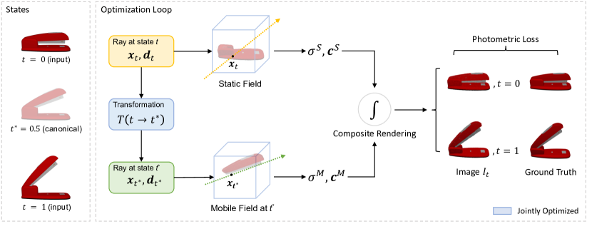
Figure 2: Method overview. We learn a part-level reconstruction in two separate fields through composite rendering supervised by images in two given states simultaneously. To render an image at input state $t$, we query the static field with the rays at $t$ to obtain the static part, then we transform the ray from $t$ to $t^{*}$ to query the mobile field which returns the corresponding points of movable part at $t$ from its canonical state. By compositing the colors from two fields, we can supervise the rendering results with the ground truth images from the input state $t$. The network and motion parameters will be jointly optimized for each specific scene.

3 Problem Statement

Considering an articulated object from an unknown category, our input is composed of two arbitrary articulation states of the object: start state $t=0$ and end state $t=1$. At each state $t$, a set of multi-view RGB images $I^{t}$ with corresponding camera parameters are given. We assume only one part is moving in this pair of observations, where we call the moving part the movable part and the part remaining still the static part. Our first goal is to decouple the two parts in terms of both geometry and appearance. With a part-level shape and appearance model in hand, we can articulate the object to unseen states and render the object in new states from arbitrary views easily with articulated motion control.

Our second goal is followed by articulated motion estimation. We assume the movable part exhibits either rotation or translation only. The motion type is required to estimate the motion parameters (joint axis and joint state). If it is not given, we first optimize the transformation as a $\mathbf{SE}(3)$ group to classify the motion type as a pre-processing step. Once the motion type is known we parameterize the joint accordingly. For a revolute joint, we parameterize it with a pivot point $\textbf{p}\in\mathbb{R}^{3}$ and a rotation in the form of a unit quaternion $\textbf{q}\in\mathbb{R}^{4},\|\textbf{q}\|=1$. For a prismatic joint, we parameterize it with the joint axis as a unit vector $\textbf{a}\in\mathbb{R}^{3},\|\textbf{a}\|=1$ and translation distance $d$ along this axis. Now we have a rotation function $f_{\textbf{p},\textbf{q}}$ and a translation function $f_{\textbf{a},d}$ using these parameters. Depending on the motion type given, one of the transformation function $T\in\{f_{\textbf{p},\textbf{q}},f_{\textbf{a},d}\}$ will be plugged into the training pipeline to optimize the motion parameters jointly.

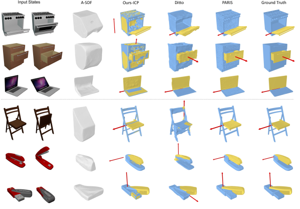
Figure 3: Qualitative results for the object and part reconstruction with joint axis visualization. Static parts are colored blue while movable parts are colored yellow. Ditto performs well in both segmentation and axis prediction in the three seen categories (above the dashed line), but the quality drops significantly for unseen categories (three cases below the dashed line). Our methods produce better segmentation with more geometric details while predicting accurate axis across all the categories.

4 Method

Our method is an end-to-end framework that learns a part-level representation and estimates articulation jointly from object-level observations in a fully self-supervised fashion. We separate the static and movable parts by leveraging motion as a cue. Since the motion accounts for the inconsistency between two states, we optimize the motion parameters by registering the moving parts from the input state $t$ to a canonical state $t^{*}$. During registration, the component that agrees with the transformation is extracted as the movable part. And the one remaining still is extracted as the static part. Figure 2 illustrates the design of our pipeline.

Next, we explain our architecture (Section 4.1), and the supervision losses (Section 4.2) in detail.

4.1 Composite Neural Radiance Fields

We learn the static and mobile fields compositely during training, and the two fields share the same network architecture which is built upon Instant-NGP [30]. Note that we design each field to model a static scene (one part in one state), meaning neither of the fields is conditioned on the state $t$ as the input. We are not modeling the continuous dynamics for the movable part since we only have multi-views of the object at two discrete states for supervision. We build the motion relation between two states by learning an explicit transformation function (defined in Section 3) that maps a canonical state to the two input states instead of relying on learned dynamics embedded in the field implicitly, which differentiates our method from other works studying the reconstruction of the dynamic scenes [48, 34]. Theoretically, any state $t$ can be chosen for the movable part. To balance the signal backpropagated from the loss on the two input states, we use $t^{*}=0.5$ as a canonical state to be learned in the field for the movable part. See the supplement for details about the choice of canonical state.

The static field $\mathcal{F}^{S}$ represents the static part that remains still in any state, and the mobile field $\mathcal{F}^{M}$ represents the movable part in the canonical state ($t^{*}=0.5$). Formally, they are represented as $\mathcal{F}^{S}(\textbf{x}_{t},\textbf{d}_{t})=\sigma^{S}(\textbf{x}_{t}),\textbf{c}^{S}(\textbf{x}_{t},\textbf{d}_{t})$ and $\mathcal{F}^{M}(\textbf{x}_{t^{*}},\textbf{d}_{t^{*}})=\sigma^{M}(\textbf{x}_{t^{*}}),\textbf{c}^{M}(\textbf{x}_{t^{*}},\textbf{d}_{t^{*}})$ where $\textbf{x}_{t}\in\mathbb{R}^{3}$ is a point sampled along a ray at state $t$ with direction, $\textbf{d}_{t}\in\mathbb{R}^{3}$. $\sigma(\textbf{x})\in\mathbb{R}$ is the density value of the point x, and $\textbf{c}(\textbf{x},\textbf{d})$ is the RGB color predicted from the point x from a view direction d. For an input state $t\in\{0,1\}$, we transform the point from $\textbf{x}_{t}$ to $\textbf{x}_{t^{*}}$ and the view direction from $\textbf{d}_{t}$ to $\textbf{d}_{t^{*}}$ to query the field $\mathcal{F}^{M}$, using the transformation function $T$ which is defined in Section 3. Learning an accurate articulation and segmentation establishes a correspondence from state $t$ to $t^{*}$.

We adopt a similar training pipeline to the original NeRF [26] and extend the ray marching and volumetric rendering procedure to compose the two fields. For each training iteration, we independently sample points to produce rendering for each input state $t\in\{0,1\}$ and supervise the results respectively. During ray marching for each state $t$, we first uniformly sample points $\textbf{x}_{t}$ along each ray to query the field $\mathcal{F}^{S}$, then we transform $\textbf{x}_{t}$ to $\textbf{x}_{t^{*}}$ to query the field $\mathcal{F}^{M}$. The summation of the output densities $\sigma_{sum}=\sigma^{S}(\textbf{x}_{t})+\sigma^{M}(\textbf{x}_{t^{*}})$ is used to construct the probability density function to guide the stratified sampling in the second round of ray marching.

		Unseen Category							Seen Category
Metrics	Methods	Stapler	USB	Scissor	Fridge	FoldChair	Washer	Blade	Laptop	Oven	Storage	Mean
CD-w$\downarrow$	A-SDF	14.19	7.14	10.61	13.71	40.85	12.50	3.31	2.11	21.37	22.57	14.84
	Ditto	2.38	2.09	1.70	2.16	6.80	7.29	42.04	0.31	2.51	3.91	7.19
	Ours-ICP	0.91	1.97	0.52	3.44	0.39	13.98	0.42	1.54	8.40	7.67	3.92
	PARIS	0.96	1.80	0.30	2.68	0.42	18.31	0.46	0.25	6.07	8.12	3.94
CD-s$\downarrow$	Ditto	41.64	2.64	39.07	3.05	33.79	10.32	46.90	0.25	2.52	9.18	18.94
	Ours-ICP	1.09	2.37	0.58	3.79	2.34	8.26	0.50	0.42	5.95	12.59	3.79
	PARIS	0.94	2.60	0.28	2.88	0.20	19.45	0.58	0.15	6.19	11.76	4.50
CD-m$\downarrow$	Ditto	31.21	15.88	20.68	0.99	141.11	12.89	195.93	0.19	0.94	2.20	42.20
	Ours-ICP	8.13	2.09	18.19	129.48	38.31	74.76	20.49	67.90	43.20	156.81	55.94
	PARIS	0.85	0.89	0.23	1.13	0.53	0.27	5.13	0.14	0.43	20.67	3.06

Table 1: Quantitative results for the surface quality of the reconstructed object and parts. We outperform other methods on the reconstruction of the whole object and movable part on average, and we have comparable quality with Ours-ICP on the static part reconstruction.

Let $\textbf{x}(h)=\textbf{o}+h\textbf{d}$ be a point along a ray $\textbf{r}=\textbf{o}+h\textbf{d}$ emitted from the center of the projection o with direction d. Considering a near and far bound $[h_{n},h_{f}]$, we composite the output from two fields to calculate the color $\hat{C}(\textbf{r})$ for the ray r by integrating the weighted sum of the two colors for each point along the ray:

$$\hat{C}(\textbf{r})=\int_{h_{n}}^{h_{f}}\left(w^{S}(h)\cdot\textbf{c}^{S}(h)+w^{M}(h)\cdot\textbf{c}^{M}(h)\right)dh$$ (1)

where we simplify our notation as $\textbf{c}(h)\equiv\textbf{c}(\textbf{x}(h),\textbf{d})$. We define the weights $w^{S}(h)=T(h)\cdot\alpha^{S}(h)$ and $w^{M}(h)=T(h)\cdot\alpha^{M}(h)$, where $T(h)$ is the transmittance at the point $\textbf{x}(h)$ accumulated from the two fields with the summation density $\sigma_{sum}(s)$. This is defined as:

$$T(h)=\exp{\left(-\int_{h_{n}}^{h}\sigma_{sum}(s)\cdot\delta_{s}\hskip 5.0ptds\right)}$$ (2)

where $\delta_{s}=h_{s+1}-h_{s}$ is the distance between adjacent samples. The intuition of this additive composition is that sample points from either field with a high-density value can terminate the ray during rendering. This strategy is also adopted in STaR [51] and D²NeRF [48].

4.2 Supervision Losses

We supervise the learning of motion parameters and neural radiance fields jointly with two shared loss functions. The overall loss function is defined as $\mathcal{L}=\mathcal{L}_{\text{rgb}}+\lambda_{\text{mask}}\mathcal{L}_{\text{mask}}$ where the optimizer for motion parameters only considers $\mathcal{L}_{\text{rgb}}$ and $\mathcal{L}_{\text{mask}}$ during training. $\mathcal{L}_{\text{rgb}}$ defines the photometric loss between the rendering RGB value with ground truth RGB value $C(\textbf{r})$ for a pixel hit by ray r:

$$\mathcal{L}_{\text{rgb}}=\|\hat{C}(\textbf{r})-C(\textbf{r})\|_{2}^{2}.$$ (3)

The mask loss $\mathcal{L}_{\text{mask}}$ is defined on the opacity $O(\textbf{r})$ for each pixel with a binary mask $M(\textbf{r})$ of the object:

$$\mathcal{L}_{\text{mask}}=\text{BCE}\left(O(\textbf{r}),M(\textbf{r})\right)$$ (4)

where BCE is the binary cross-entropy loss and $\lambda_{\text{mask}}=0.1$ during training. The opacity $O(\textbf{r})$ is computed as:

$$O(\textbf{r})=\int_{h_{n}}^{h_{f}}w(h)\hskip 5.0ptdh.$$ (5)

We empirically find that the mobile field easily accumulates noise in regions overlapping with the static field, especially when the static part is a large volume. The static part hides noise inside its volume during composition and we lack supervision on the points behind the surface with volumetric rendering. To alleviate this problem, we add a regularization term $\mathcal{L}_{\text{prob}}$. The intuition is to encourage the composited color for each ray to be only contributed from one field instead of both. We define the ratio that the color of a ray r contributed from the mobile field as a fraction of the opacity values:

$$P_{M}(\textbf{r})=\frac{O^{M}(\textbf{r})}{O^{M}(\textbf{r})+O^{S}(\textbf{r})}.$$ (6)

Then we define our regularization term $\mathcal{L}_{prob}$ on this ratio for each ray as:

$$\mathcal{L}_{\text{prob}} =H(P_{M}(\textbf{r})),$$ (7)

$$H(x) =x\cdot\log(x)+(1-x)\cdot\log(1-x).$$ (8)

By minimizing $\mathcal{L}_{\text{prob}}$ for all the pixels in each iteration, we force $P_{M}(\textbf{r})$ to be close to either 0 or 1. Thus, the density for each position will be encouraged to accumulate in only one field. We weigh this regularization term with $0.001$ and only apply it to the loss for optimizing parameters for implicit fields as it does not provide a meaningful signal for motion estimation.

5 Experiments

		Revolute								Prismatic
Metrics	Methods	Stapler	USB	Scissor	Fridge	FoldChair	Washer	Oven	Laptop	Blade	Storage	Mean
Ang Err$\downarrow$	Ditto	89.86	89.77	4.498	89.30*	89.35	89.51	0.955	3.124	6.319	79.54*	54.22
	Ours-ICP	0.179	1.142	0.528	5.192	0.256	89.20	74.94	0.488	80.71	22.33	27.50
	PARIS	0.069	0.065	0.019	0.001	0.020	0.082	0.028	0.034	0.001	0.369	0.069
Pos Err$\downarrow$	Ditto	0.201	5.409	5.698	1.021*	3.768	0.661	0.129	0.014	-	-	2.113
	Ours-ICP	0.073	0.183	0.000	2.965	0.000	2.427	9.035	0.047	-	-	1.841
	PARIS	0.006	0.000	0.000	0.002	0.004	0.02	0.003	0.001	-	-	0.005

Table 2: Quantitative results for evaluating the error in joint axis prediction. We perform the best across the 10 examples. Ditto achieves four comparable estimations, four wrong ones, and two with the wrong motion type (marked with $*$). Ours-ICP performs in between.

	Revolute									Prismatic
Methods	Stapler	USB	Scissor	Fridge	FoldChair	Washer	Oven	Laptop	Mean	Blade	Storage	Mean
Ditto	56.61	80.60	19.28	F	99.36	55.72	2.094	5.181	50.89	F	0.086	0.086
Ours-ICP	0.423	1.704	0.364	11.39	0.465	175.1	68.48	0.668	32.32	0.262	0.311	0.287
PARIS	0.000	0.028	0.000	0.001	0.000	0.079	0.000	0.028	0.017	0.064	0.000	0.032

Table 3: Estimation for the joint state - we measure the geodesic distance $\downarrow$ (degree) for revolute joints and translation error $\downarrow$ for prismatic joints. We can predict significantly accurate rotation angles for revolute joints, and also performs better for prismatic joints. The cases with the wrong motion type predicted by Ditto are denoted as F.

5.1 Dataset

Synthetic dataset. The synthetic 3D models we use for evaluation are from the PartNet-Mobility dataset [49, 27, 4], a large-scale dataset for articulated objects across 46 categories. We select instances across 10 categories to conduct our experiments. For each articulation state, we randomly sample 64-100 views covering the upper hemisphere of the object to simulate capturing in the real world. Then we render RGB images and acquire camera parameters and object masks using Blender [6] to create our training data.

Real-world dataset. The real data we use for experiments is from the MultiScan dataset [25], scanning real-world indoor scenes with articulated objects in multiple states. We use the reconstructed mesh of an object in two states as ground truth for evaluation, and the real RGB frames as training data.

5.2 Baselines

A-SDF. A-SDF [29] learns a category-level model that reconstructs object meshes given ground truth SDF samples. To compare the generalization ability of the model across categories, we train the model on the 10 testing examples and retrieve them during testing. We follow the method that DeepSDF [32] proposed to generate SDF samples for each testing case. Note that A-SDF cannot predict part-level geometry or estimate explicit motion parameters, we only measure the quality of surface reconstruction on the whole object for comparison.

Ditto. Ditto [20] learns a category-agnostic model that reconstructs part meshes and estimates motion parameters (motion type, joint axis, joint state) from a pair of 3D point clouds. We leverage their released pre-trained model which is trained on Shape2Motion [45] dataset across 4 categories to do the comparison. And we test instances across 10 categories (3 seen and 7 unseen by Ditto, marked in Table 1) to compare the generalization ability regarding the part-level surface reconstruction and motion estimation. We sample point clouds on the surface of the ground truth meshes of the object in two given articulation states to feed as their input for both synthetic and real data experiments.

Ours-ICP. None of the baseline methods mentioned above can produce the appearance of the object or even render the object in arbitrary views since they did not consume RGB information as their input. Here, we implemented a naive baseline approach as illustrated in Figure 4. We learn two separate neural implicit surfaces $F_{0},F_{1}$ from the two given sets of multi-view images, which are backboned with NeuS [44] and Instant-NGP [30]. Then we compare the quality of the novel view synthesis at two given articulated states with this baseline model. Additionally, we apply Constructive Solid Geometry (CSG) algorithm between the two neural SDFs and extract the part-level geometry with Marching-Cube [24]. Specifically, the intersection region of the two fields can be extracted as the static part. By subtracting one field from the other, we can obtain the movable part in two states accordingly. We can further compute the transformation between the movable parts in two states by using global registration [36, 10, 40] and generalized ICP registration [38] algorithms.

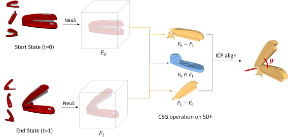
Figure 4: Pipeline of our baseline method Ours-ICP. We learn separate neural SDFs $F_{0},F_{1}$ for the object in state $t=\{0,1\}$. To segment static and movable parts, we apply CSG operations between two SDFs. Then we leverage global registration and the ICP algorithm to obtain the transformation on the movable parts from the start to end state.

5.3 Evaluation Metrics

Part-level geometry. We use the Chamfer-L1 distance (CD) as the metric to evaluate the quality of the reconstructed meshes. We measure the CD on the whole reconstructed surface (CD-w) to compare it with all the baselines. We also measure the CD on the predicted static part (CD-s) and movable part (CD-m) separately to compare them with all the baselines except for A-SDF since it cannot predict part segmentation without ground truth SDFs for parts. To be more specific, we sample 10,000 points on each surface to compute the distance from both the prediction to the ground truth and the other way around, then we average the two distances to report as the final metrics. The CD values shown are multiplied by 1,000 as in A-SDF and Ditto.

Motion estimation. To evaluate the joint axis, we measure the angular error (Ang Err) for both types of joints. This metric computes the orientation difference between the predicted axis direction and the ground truth, ranging from 0 to 90 degrees. We also measure the position error (Pos Err) for revolute joints. This metric computes the minimum distance between the rotation axis and the ground truth which takes the position of the pivot point into account. The value is multiplied by 10 shown in Table 2. To evaluate the joint state, we measure the geodesic distance (in degree) for revolute joints and translation error for prismatic joints.

Novel view synthesis. To evaluate the quality of the appearance model, we measure the Peak Signal-to-noise Ratio (PSNR) and the Structural Similarity Index (SSIM) [46] for rendered results from novel views. For each instance, we render 50 novel views of the object in each state and average the values. We achieve comparable rendering quality with the ICP baseline. See the supplement for details.

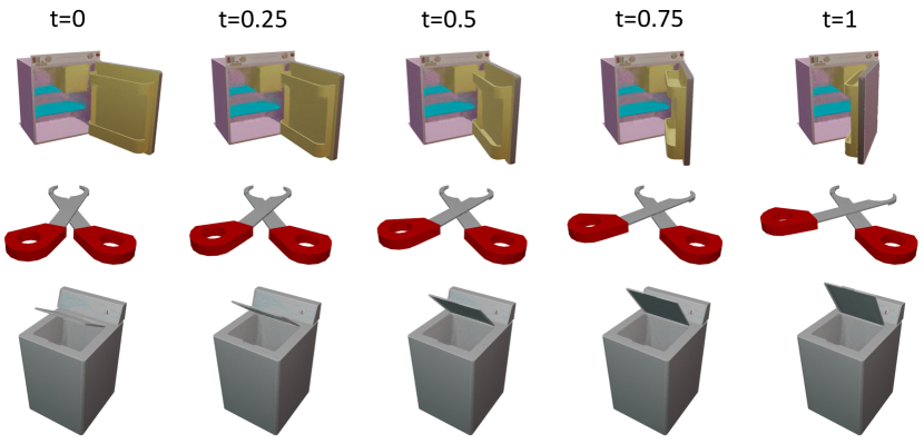
Figure 5: Rendering of unseen states from an arbitrary novel view by interpolating $t$ as input. Our high-quality results demonstrate that our motion prediction and decoupling of the part appearance are accurate to effectively generate arbitrary unseen states.

5.4 Experiment Results

Reconstruction and part segmentation. The quantitative results are in Table 1 and a qualitative comparison is in Figure 3. Note that our method reconstructs the canonical state of the movable part as the output, whereas Ditto [20] outputs the start state. Thus, we transform our predicted movable part from the canonical state to the start state using the predicted motion for these results.

For the whole object reconstruction, we observe in Table 1 that Ditto outperforms for Fridge, Washer, Oven, and Storage. Since Ditto takes ground truth 3D point clouds as input, they have more information about the inner space of these objects than we do with limited image views. So it is understandable that they perform better when a deep container is involved. For part segmentation, we outperform 7 out of 10 cases for both the static and movable parts. We have a big improvement over the movable part on average and outperform the baselines on average. From Table 1, we observe that Ditto performs well in the three seen categories (above the dashed line), but the quality drops significantly for unseen categories (below the dashed line). Also, we produce more geometric details and better segmentation, which indicates we have a better generalization ability.

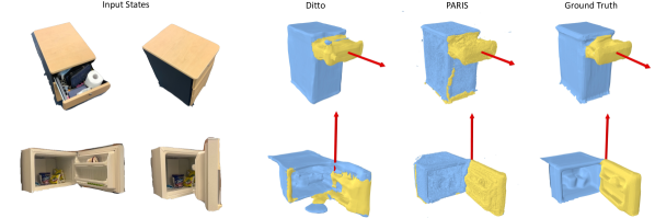
Figure 6: Qualitative results for two real-world objects. Ditto and our method can both estimate accurate motion parameters. Ditto produces cleaner segmentation in the first case, but a less accurate geometry in the second case.

Motion estimation. We show the quantitative results of the joint axis and joint state estimation in Table 2 and Table 3. The predicted axis is also visualized in Figure 3. We observe that our motion estimation is significantly more accurate than other baselines for both revolute and prismatic joints. Since Ditto predicts a wrong motion type for two of the testing examples, we report a failure (F) in Table 3 for joint state evaluation and denote $*$ beside the numbers in Table 2 for joint axis evaluation.

Novel view synthesis and articulation generation. We show the qualitative results of generating the intermediate articulation using the motion we predict from an arbitrary view in Figure 5. Our high-quality rendering results for the intermediate states demonstrate that our decoupling of the part appearance model is accurate, and we can effectively generate arbitrary unseen states and render from arbitrary views with our part-level implicit representation and predicted motion parameters.

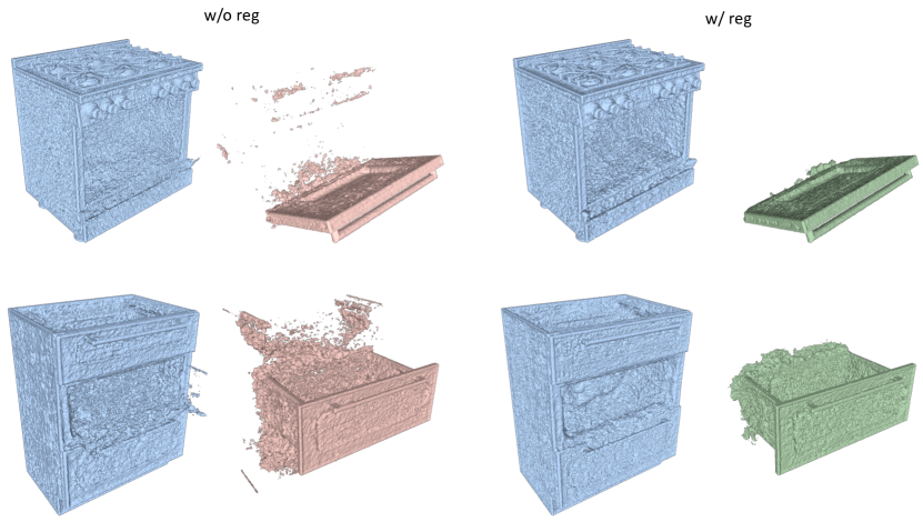
Figure 7: Ablation of our regularization term. The left two columns show part reconstruction without this term, and the right two columns show the result with the term added. Note the reduction in movable part noise.

	Geometry			Motion				Appearance
Method	CD-w$\downarrow$	CD-s$\downarrow$	CD-m$\downarrow$	Ang$\downarrow$	Pos$\downarrow$	Geo$\downarrow$	Trans$\downarrow$	PSNR$\uparrow$	SSIM$\uparrow$
w/o reg	4.78	4.97	23.32	0.087	0.006	0.029	0.054	36.64	0.989
w/ reg	3.93	4.50	5.38	0.069	0.005	0.017	0.032	37.73	0.992

Table 4: Ablation for the regularization term. Geometry, motion, and appearance all improve when using regularization.

Ablation studies. We conduct an ablation for the effectiveness of the regularization term in improving reconstruction quality, motion estimation, and appearance. The results are in Table 4. We observe that the regularization can indeed improve the surface reconstruction for both part and object on average, especially for the movable part where we do not have sufficient views to observe the whole part (e.g., Washer, Oven). We also show qualitative results in Figure 7 to have a closer look at the changes in the movable part for the two most effective cases.

We have an ablation for the choice of canonical state reconstructed in the mobile field. We choose to reconstruct a “virtual” state at $t^{*}=0.5$ in our pipeline. This better fits our problem statement as it allows us to utilize supervision signals from both given states to predict the motion and segmentation. In Table 6, we show the impact on performance of using given state $t^{*}=0$ (more similar to STaR[51]) as the canonical state instead. We note a performance reduction across all aspects except for appearance for which the results are comparable, with a particularly large degradation in movable part geometric accuracy.

We also carry out an ablation over the number of input views by downsampling the views with farthest point sampling. In Table 7, we reproduce 64 view results from Tables 1, 2 and 3 and report results for 32 to 4 views. We observe a decline in performance with decreasing views, with a significant drop below 16 views. This is expected given the challenge of learning NeRFs in the few input regime, and constitutes an interesting direction for future work.

		Geometry			Motion
Example	Method	CD-w$\downarrow$	CD-s$\downarrow$	CD-m$\downarrow$	Ang$\downarrow$	Pos$\downarrow$	Geo$\downarrow$	Trans$\downarrow$
Fridge	Ditto	6.50	47.01	50.60	1.71	1.84	8.43	-
	PARIS	8.20	10.22	67.54	1.91	0.53	0.77	-
Storage	Ditto	14.08	16.09	20.35	5.88	-	-	0.38
	PARIS	18.98	20.92	101.20	3.88	-	-	0.31

Table 5: Quantitative results for real-world objects. We produce comparable quality surfaces for the static part and object as a whole compared to Ditto, but less accurate surfaces for movable parts. Our motion estimation is better.

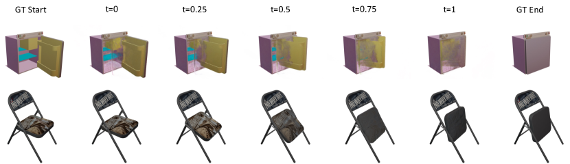
Figure 8: Failure cases of articulation generation with incorrectly predicted motion. This figure illustrates how our predicted motion manipulates the movable part to satisfy the supervision in the wrong way. The door of the fridge is wrongly rotating around an axis away from the body, and the seat of the chair is rotating around the correct joint axis but in an opposite direction.

Real-world examples. Comparison with Ditto for two real cases is shown in Figure 6 and Table 5. Since Ditto and our method both assume that the geometries of the object in two states are pre-aligned, we both suffer from the error in alignment and reconstruction on the given mesh. Ditto and our method can both estimate accurate motion parameters. Ditto produces cleaner segmentation in the first case, but a less accurate geometry in the second case.

5.5 Limitations

To obtain an accurate decoupling of the parts and motion parameters, our method relies on a sufficient number of multi-view observations of the object for both static and movable parts. Our inputs exhibit occlusions both across views (tightly connected parts) and between states (e.g. in Figure 1 end state, a large portion of the static part is occluded). This increases the level of difficulty in finding 3D correspondence from RGB images only. We observe that our method tends to fail to estimate the correct motion parameters for revolute joints when the movable part is 1) severely occluded across views (e.g., the door of the cabinet is fully closed); or 2) highly geometrically symmetric. We illustrate these failure modes in Figure 8 by rendering objects from a novel view in sequential states. This figure illustrates how our predicted motion manipulates the movable part to satisfy the supervision at two given states in the wrong way. Specifically, the door of the fridge is wrongly rotating around an axis away from the body, and the seat of the chair is rotating around the correct joint axis but in an opposite direction. We also observe that the optimization on the very thin parts is inclined to be unstable which can be alleviated by increasing the number of viewpoints.

	Geometry			Motion				Appearance
canonical	CD-w$\downarrow$	CD-s$\downarrow$	CD-m$\downarrow$	Ang$\downarrow$	Pos$\downarrow$	Geo$\downarrow$	Trans$\downarrow$	PSNR$\uparrow$	SSIM$\uparrow$
$t^{*}=0.5$	3.94	4.50	3.06	0.069	0.005	0.017	0.032	37.73	0.992
$t^{*}=0$	13.25	5.64	74.34	0.070	0.005	0.050	0.088	37.62	0.992

Table 6: Ablation of canonical state selection. We note a performance reduction across all aspects, with a particularly large degradation in movable part geometric accuracy.

	Geometry			Motion				Appearance
# views	CD-w$\downarrow$	CD-s$\downarrow$	CD-m$\downarrow$	Ang$\downarrow$	Pos$\downarrow$	Geo$\downarrow$	Trans$\downarrow$	PSNR$\uparrow$	SSIM$\uparrow$
64	3.94	4.50	3.06	0.069	0.005	0.017	0.032	37.73	0.992
32	4.053	4.841	19.482	0.181	0.041	11.346	0.033	34.36	0.986
16	6.677	6.479	35.459	4.542	0.638	14.447	0.039	30.24	0.975
8	54.784	64.040	196.86	36.990	2.093	29.432	0.116	19.29	0.918
4	170.116	220.030	286.600	37.721	3.212	29.797	0.150	16.83	0.886

Table 7: Ablation of input view number. We observe a decline in performance with decreasing views, with a significant drop below 16 views.

6 Conclusion

We addressed the task of joint part-level shape and appearance reconstruction and motion parameter estimation for articulated objects. Our work is the first to tackle this task from multi-view RGB images observing the object in two arbitrary states. We evaluated our method on synthetic and real data to systematically study the challenges in this task. Our experiments show that we can recover shape, appearance, and motion parameters better than prior work and baselines. However, the task remains challenging especially for cases with severe occlusion. Extending to objects with multiple parts is another challenge for future work. Moreover, we assumed the two given object states are aligned in world coordinates, an assumption shared with prior work. We hope our work inspires more research into articulated object reconstruction without 3D supervision.

Acknowledgements. This work was funded in part by a Canada Research Chair grant (CRC-2019-00298), NSERC Discovery grants (RGPIN-2019-06489, RGPIN-2022-03111), and NSERC Discovery Launch Supplement (DGECR-2022-00359), and enabled in part by support from WestGrid and Compute Canada. We thank Hanxiao Jiang, Han-Hung Lee, Yongsen Mao, Yilin Liu for helpful discussions, as well as Angel X. Chang, Sanjay Haresh, Ning Wang, and Qirui Wu for proofreading.

References

- Abbatematteo et al. [2020] Ben Abbatematteo, Stefanie Tellex, and George Konidaris. Learning to generalize kinematic models to novel objects. In Proceedings of the Conference on Robot Learning, volume 100, pages 1289–1299, 2020.
- [2] Hameed Abdul-Rashid, Miles Freeman, Ben Abbatematteo, George Dimitri Konidaris, and Daniel Ritchie. Learning to infer kinematic hierarchies for novel object instances. Proceedings of the International Conference on Robotics and Automation (ICRA).
- Barron et al. [2022] Jonathan T. Barron, Ben Mildenhall, Dor Verbin, Pratul P. Srinivasan, and Peter Hedman. Mip-NeRF 360: Unbounded anti-aliased neural radiance fields. In Proceedings of the IEEE Conference on Computer Vision and Pattern Recognition (CVPR), pages 5460–5469, 2022.
- Chang et al. [2015] Angel X. Chang, Thomas A. Funkhouser, Leonidas J. Guibas, Pat Hanrahan, Qi-Xing Huang, Zimo Li, Silvio Savarese, Manolis Savva, Shuran Song, Hao Su, Jianxiong Xiao, Li Yi, and Fisher Yu. ShapeNet: An information-rich 3D model repository. CoRR, abs/1512.03012, 2015.
- Chu et al. [2023] Ruihang Chu, Zhengzhe Liu, Xiaoqing Ye, Xiao Tan, Xiaojuan Qi, Chi-Wing Fu, and Jiaya Jia. Command-driven articulated object understanding and manipulation. In Proceedings of the IEEE Conference on Computer Vision and Pattern Recognition (CVPR), pages 8813–8823, 2023.
- Community [2018] Blender Online Community. Blender - a 3D modelling and rendering package. Blender Foundation, Stichting Blender Foundation, Amsterdam, 2018. URL http://www.blender.org.
- de Goes et al. [2022] Fernando de Goes, William Sheffler, and Kurt Fleischer. Character articulation through profile curves. ACM Transactions on Graphics, 41(4):139:1–139:14, 2022.
- Deng et al. [2020] Boyang Deng, JP Lewis, Timothy Jeruzalski, Gerard Pons-Moll, Geoffrey Hinton, Mohammad Norouzi, and Andrea Tagliasacchi. NASA: Neural articulated shape approximation. In Proceedings of the European Conference on Computer Vision (ECCV), volume 12352, pages 612–628, 2020.
- Fan et al. [2023] Zicong Fan, Omid Taheri, Dimitrios Tzionas, Muhammed Kocabas, Manuel Kaufmann, Michael J. Black, and Otmar Hilliges. ARCTIC: A dataset for dexterous bimanual hand-object manipulation. In Proceedings of the IEEE Conference on Computer Vision and Pattern Recognition (CVPR), 2023.
- Fischler and Bolles [1981] Martin A. Fischler and Robert C. Bolles. Random sample consensus: A paradigm for model fitting with applications to image analysis and automated cartography. Commun. ACM, 24(6):381–395, 1981.
- Gadre et al. [2021] Samir Yitzhak Gadre, Kiana Ehsani, and Shuran Song. Act the part: Learning interaction strategies for articulated object part discovery. In Proceedings of the IEEE/CVF International Conference on Computer Vision (ICCV), pages 15752–15761, October 2021.
- Gao et al. [2020] Jun Gao, Wenzheng Chen, Tommy Xiang, Alec Jacobson, Morgan McGuire, and Sanja Fidler. Learning deformable tetrahedral meshes for 3D reconstruction. In Advances in neural information processing systems, 2020.
- Guo et al. [2022] Xiang Guo, Guanying Chen, Yuchao Dai, Xiaoqing Ye, Jiadai Sun, Xiao Tan, and Errui Ding. Neural deformable voxel grid for fast optimization of dynamic view synthesis. In Proceedings of the Asian Conference on Computer Vision (ACCV), 2022.
- Haresh et al. [2022] Sanjay Haresh, Xiaohao Sun, Hanxiao Jiang, Angel X. Chang, and Manolis Savva. Articulated 3D human-object interactions from RGB videos: An empirical analysis of approaches and challenges. In 3DV, pages 312–321, 2022.
- Heppert et al. [2023] Nick Heppert, Muhammad Zubair Irshad, Sergey Zakharov, Katherine Liu, Rares Andrei Ambrus, Jeannette Bohg, Abhinav Valada, and Thomas Kollar. CARTO: Category and joint agnostic reconstruction of articulated objects. In Proceedings of the IEEE Conference on Computer Vision and Pattern Recognition (CVPR), pages 21201–21210, 2023.
- Hsu et al. [2023] Cheng-Chun Hsu, Zhenyu Jiang, and Yuke Zhu. Ditto in the house: Building articulation models of indoor scenes through interactive perception. 2023.
- Hu et al. [2017] Ruizhen Hu, Wenchao Li, Oliver Van Kaick, Ariel Shamir, Hao Zhang, and Hui Huang. Learning to predict part mobility from a single static snapshot. ACM Transactions on Graphics, 36(6):1–13, 2017.
- Jain et al. [2021] Ajinkya Jain, Rudolf Lioutikov, Caleb Chuck, and Scott Niekum. ScrewNet: Category-independent articulation model estimation from depth images using screw theory. In Proceedings of the International Conference on Robotics and Automation (ICRA), pages 13670–13677, 2021.
- Jain et al. [2019] Rishabh Jain, Mohd. Nayab Zafar, and J. C. Mohanta. Modeling and analysis of articulated robotic arm for material handling applications. IOP Conference Series: Materials Science and Engineering, 691(1):012010, nov 2019.
- Jiang et al. [2022] Zhenyu Jiang, Cheng-Chun Hsu, and Yuke Zhu. Ditto: Building Digital Twins of Articulated Objects from Interaction. In Proceedings of the IEEE Conference on Computer Vision and Pattern Recognition (CVPR), pages 5606–5616, 2022.
- Li et al. [2020] Xiaolong Li, He Wang, Li Yi, Leonidas Guibas, A Lynn Abbott, and Shuran Song. Category-level articulated object pose estimation. Proceedings of the IEEE Conference on Computer Vision and Pattern Recognition (CVPR), pages 3703–3712, 2020.
- Liu et al. [2023] Gengxin Liu, Qian Sun, Haibin Huang, Chongyang Ma, Yulan Guo, Li Yi, Hui Huang, and Ruizhen Hu. Semi-weakly supervised object kinematic motion prediction. In Proceedings of the IEEE Conference on Computer Vision and Pattern Recognition (CVPR), pages 21726–21735, 2023.
- Liu et al. [2022] Liu Liu, Wenqiang Xu, Haoyuan Fu, Sucheng Qian, Qiaojun Yu, Yang Han, and Cewu Lu. AKB-48: A real-world articulated object knowledge base. In Proceedings of the IEEE Conference on Computer Vision and Pattern Recognition (CVPR), pages 14789–14798, 2022.
- Lorensen and Cline [1987] William E. Lorensen and Harvey E. Cline. Marching Cubes: A high resolution 3D surface construction algorithm. In Proc. SIGGRAPH, pages 163–169, 1987.
- Mao et al. [2022] Yongsen Mao, Yiming Zhang, Hanxiao Jiang, Angel X Chang, and Manolis Savva. MultiScan: Scalable RGBD scanning for 3D environments with articulated objects. In Advances in neural information processing systems, 2022.
- Mildenhall et al. [2020] Ben Mildenhall, Pratul P. Srinivasan, Matthew Tancik, Jonathan T. Barron, Ravi Ramamoorthi, and Ren Ng. NeRF: Representing scenes as neural radiance fields for view synthesis. In Proceedings of the European Conference on Computer Vision (ECCV), pages 405–421, 2020.
- Mo et al. [2019] Kaichun Mo, Shilin Zhu, Angel X. Chang, Li Yi, Subarna Tripathi, Leonidas J. Guibas, and Hao Su. PartNet: A large-scale benchmark for fine-grained and hierarchical part-level 3D object understanding. In Proceedings of the IEEE Conference on Computer Vision and Pattern Recognition (CVPR), pages 909–918, 2019.
- Mo et al. [2021] Kaichun Mo, Leonidas J. Guibas, Mustafa Mukadam, Abhinav Gupta, and Shubham Tulsiani. Where2Act: From pixels to actions for articulated 3D objects. In Proceedings of the IEEE International Conference on Computer Vision (ICCV), pages 6793–6803, 2021.
- Mu et al. [2021] Jiteng Mu, Weichao Qiu, Adam Kortylewski, Alan Yuille, Nuno Vasconcelos, and Xiaolong Wang. A-sdf: Learning disentangled signed distance functions for articulated shape representation. In Proceedings of the IEEE International Conference on Computer Vision (ICCV), pages 12981–12991, 2021.
- Müller et al. [2022] Thomas Müller, Alex Evans, Christoph Schied, and Alexander Keller. Instant neural graphics primitives with a multiresolution hash encoding. ACM Transactions on Graphics, 41(4):102:1–102:15, 2022.
- Noguchi et al. [2021] Atsuhiro Noguchi, Xiao Sun, Stephen Lin, and Tatsuya Harada. Neural articulated radiance field. In Proceedings of the IEEE International Conference on Computer Vision (ICCV), pages 5742–5752, 2021.
- Park et al. [2019] Jeong Joon Park, Peter Florence, Julian Straub, Richard Newcombe, and Steven Lovegrove. DeepSDF: Learning continuous signed distance functions for shape representation. In Proceedings of the IEEE Conference on Computer Vision and Pattern Recognition (CVPR), pages 165–174, 2019.
- Park et al. [2021] Keunhong Park, Utkarsh Sinha, Peter Hedman, Jonathan T. Barron, Sofien Bouaziz, Dan B Goldman, Ricardo Martin-Brualla, and Steven M. Seitz. HyperNeRF: A higher-dimensional representation for topologically varying neural radiance fields. ACM Transactions on Graphics, 40(6):238:1–238:12, 2021.
- Pumarola et al. [2021] Albert Pumarola, Enric Corona, Gerard Pons-Moll, and Francesc Moreno-Noguer. D-NeRF: Neural radiance fields for dynamic scenes. In Proceedings of the IEEE Conference on Computer Vision and Pattern Recognition (CVPR), pages 10318–10327, 2021.
- Qi et al. [2017] Charles Ruizhongtai Qi, Li Yi, Hao Su, and Leonidas J. Guibas. PointNet++: Deep hierarchical feature learning on point sets in a metric space. In Advances in neural information processing systems, pages 5099–5108, 2017.
- Rusu et al. [2009] Radu Bogdan Rusu, Nico Blodow, and Michael Beetz. Fast point feature histograms (FPFH) for 3D registration. In Proceedings of the International Conference on Robotics and Automation (ICRA), pages 3212–3217, 2009.
- Savva et al. [2019] Manolis Savva, Abhishek Kadian, Oleksandr Maksymets, Yili Zhao, Erik Wijmans, Bhavana Jain, Julian Straub, Jia Liu, Vladlen Koltun, Jitendra Malik, et al. Habitat: A platform for embodied ai research. In Proceedings of the IEEE International Conference on Computer Vision (ICCV), pages 9339–9347, 2019.
- Segal et al. [2009] Aleksandr V. Segal, Dirk Hähnel, and Sebastian Thrun. Generalized-ICP. In Robotics: Science and Systems, 2009.
- Siarohin et al. [2021] Aliaksandr Siarohin, Oliver J. Woodford, Jian Ren, Menglei Chai, and Sergey Tulyakov. Motion representations for articulated animation. In Proceedings of the IEEE Conference on Computer Vision and Pattern Recognition (CVPR), pages 13653–13662, 2021.
- Sungjoon Choi et al. [2015] Sungjoon Choi, Qian-Yi Zhou, and Vladlen Koltun. Robust reconstruction of indoor scenes. In Proceedings of the IEEE Conference on Computer Vision and Pattern Recognition (CVPR), pages 5556–5565, 2015.
- Szot et al. [2021] Andrew Szot, Alexander Clegg, Eric Undersander, Erik Wijmans, Yili Zhao, John Turner, Noah Maestre, Mustafa Mukadam, Devendra Singh Chaplot, Oleksandr Maksymets, Aaron Gokaslan, Vladimír Vondruš, Sameer Dharur, Franziska Meier, Wojciech Galuba, Angel Chang, Zsolt Kira, Vladlen Koltun, Jitendra Malik, Manolis Savva, and Dhruv Batra. Habitat 2.0: Training home assistants to rearrange their habitat. In Advances in neural information processing systems, volume 34, pages 251–266, 2021.
- Tretschk et al. [2021] Edgar Tretschk, Ayush Tewari, Vladislav Golyanik, Michael Zollhöfer, Christoph Lassner, and Christian Theobalt. Non-rigid neural radiance fields: Reconstruction and novel view synthesis of a dynamic scene from monocular video. In Proceedings of the IEEE International Conference on Computer Vision (ICCV), pages 12939–12950, 2021.
- Tseng et al. [2022] Wei-Cheng Tseng, Hung-Ju Liao, Lin Yen-Chen, and Min Sun. CLA-NeRF: Category-Level Articulated Neural Radiance Field. In Proceedings of the International Conference on Robotics and Automation (ICRA), pages 8454–8460, 2022.
- Wang et al. [2021] Peng Wang, Lingjie Liu, Yuan Liu, Christian Theobalt, Taku Komura, and Wenping Wang. NeuS: Learning neural implicit surfaces by volume rendering for multi-view reconstruction. In Marc’Aurelio Ranzato, Alina Beygelzimer, Yann N. Dauphin, Percy Liang, and Jennifer Wortman Vaughan, editors, Advances in neural information processing systems, pages 27171–27183, 2021.
- Wang et al. [2019] Xiaogang Wang, Bin Zhou, Yahao Shi, Xiaowu Chen, Qinping Zhao, and Kai Xu. Shape2Motion: Joint analysis of motion parts and attributes from 3D shapes. In Proceedings of the IEEE Conference on Computer Vision and Pattern Recognition (CVPR), pages 8876–8884, 2019.
- Wang et al. [2004] Zhou Wang, A.C. Bovik, H.R. Sheikh, and E.P. Simoncelli. Image quality assessment: from error visibility to structural similarity. IEEE Transactions on Image Processing, 13(4):600–612, 2004.
- Wei et al. [2022] Fangyin Wei, Rohan Chabra, Lingni Ma, Christoph Lassner, Michael Zollhoefer, Szymon Rusinkiewicz, Chris Sweeney, Richard Newcombe, and Mira Slavcheva. Self-supervised Neural Articulated Shape and Appearance Models. In Proceedings of the IEEE Conference on Computer Vision and Pattern Recognition (CVPR), pages 15795–15805, 2022.
- Wu et al. [2022] Tianhao Wu, Fangcheng Zhong, Andrea Tagliasacchi, Forrester Cole, and Cengiz Oztireli. D2NeRF: Self-supervised decoupling of dynamic and static objects from a monocular video. In Advances in neural information processing systems, 2022.
- Xiang et al. [2020] Fanbo Xiang, Yuzhe Qin, Kaichun Mo, Yikuan Xia, Hao Zhu, Fangchen Liu, Minghua Liu, Hanxiao Jiang, Yifu Yuan, He Wang, Li Yi, Angel X. Chang, Leonidas J. Guibas, and Hao Su. SAPIEN: A simulated part-based interactive environment. In Proceedings of the IEEE Conference on Computer Vision and Pattern Recognition (CVPR), pages 11094–11104, 2020.
- Yan et al. [2019] Zihao Yan, Ruizhen Hu, Xingguang Yan, Luanmin Chen, Oliver van Kaick, Hao Zhang, and Hui Huang. RPM-Net: recurrent prediction of motion and parts from point cloud. ACM Transactions on Graphics, 38(6):240:1–240:15, 2019.
- Yuan et al. [2021] Wentao Yuan, Zhaoyang Lv, Tanner Schmidt, and Steven Lovegrove. STaR: Self-supervised tracking and reconstruction of rigid objects in motion with neural rendering. In Proceedings of the IEEE Conference on Computer Vision and Pattern Recognition (CVPR), pages 13144–13152, 2021.
- Zhao et al. [2021] Hengshuang Zhao, Li Jiang, Jiaya Jia, Philip HS Torr, and Vladlen Koltun. Point transformer. In Proceedings of the IEEE International Conference on Computer Vision (ICCV), pages 16259–16268, 2021.