Transport signatures of Bogoliubov Fermi surfaces in normal metal/time-reversal symmetry broken $d$-wave superconductor junctions

Abstract

In recent times, Bogoliubov Fermi surfaces (BFSs) in superconductors (SCs) have drawn significant attention due to a substantial population of Bogoliubov quasiparticles (BQPs) together with Cooper pairs (CPs) in them. The BQPs as zero energy excitations give rise to captivating and intricate charge dynamics within the BFSs. In this theoretical study, we propose to reveal the unique signatures of the topologically protected BFSs in a normal metal/time-reversal symmetry (TRS) broken $d$-wave SC, in terms of the differential conductance and Fano factor (FF). For an isotropic $d$-wave SC, an enhancement in zero-bias conductance (ZBC) can be identified as a key signature of BFSs. However, for the anisotropic SC, this feature does not replicate due to the presence of the localized Andreev bound state (ABS) at the interface. The interplay of ABS and BFSs gives rise to an anomalous behavior in ZBC. We explain this anomalous behavior by analyzing the effective charge of the carriers in terms of the FF. The simplicity of our setup based on $d$-wave SC makes our proposal persuasive.

Introduction- The appearance of the gap in the Bogoliubov quasiparticle (BQP) spectrum is a characteristic property of conventional Bardeen-Cooper-Schrieffer (BCS) SCs Bardeen et al. (1957). For many unconventional SCs, this gap in the momentum space vanishes either at specific point nodes or along line nodes whose dimensions are always less than the dimension of the underlying normal state Fermi surface (FS) Sigrist and Ueda (1991). However, the density of BQPs at these nodes appear to be very low. Very recently, FS with same dimensions as that of the underlying normal state FS and substantially enhanced density of states, have been theoretically proposed by Agterberg et al.  Agterberg et al. (2017a). Interestingly, these FSs known as Bogoliubov Fermi surfacess (BFSs), are topologically protected by certain combinations of discrete symmetries and characterized by a $\mathcal{Z}_{2}$ topological invariant.

In literature, the concept of BFS was first proposed in time-reversal symmetry (TRS)-broken and inversion-symmetric multiband SCs with total angular momentum $j=3/2$ Agterberg et al. (2017a). From several followup works, the general prescription for the appearance of BFSs is provided as: SCs possessing additional degrees of freedom (e.g. orbital or sublattice) other than spin, host interband pairings, out of which a pseudomagnetic field appears and causes BFSs Agterberg et al. (2017a); Brydon et al. (2018); Menke et al. (2019); Sumita et al. (2019); Lapp et al. (2020); Tamura et al. (2020); Oh et al. (2021); Kim et al. (2021); Dutta et al. (2021); Zhu et al. (2021); Bhattacharya and Timm (2023); Miki et al. (2023). Furthermore, BFSs are also shown to exist together with odd-frequency pairing in $j=3/2$ SCs Dutta et al. (2021). The presence of inversion symmetry is crucial for the $\mathcal{Z}_{2}$ invariant Brydon et al. (2018); Timm and Bhattacharya (2021); Agterberg et al. (2017a); Bzdušek and Sigrist (2017). By contrast, the existence of BFSs is also investigated in non-centrosymmetric SCs Timm et al. (2021, 2017); Link and Herbut (2020) since inversion-symmetry can bring instability to BFSs under generic attractive interactions between BQPs Herbut and Link (2021); Oh and Moon (2020); Tamura et al. (2020); Link et al. (2020). In addition to $j=3/2$ SCs, BFSs are also proposed to exist in TRS-broken spin-$1/2$ SCs Setty et al. (2020a); Cao et al. (2023); Banerjee et al. (2022). Explicitly, SCs with interband pairing Setty et al. (2020b) and with large supercurrents Fulde (1965); Setty et al. (2020a) are shown to host BFSs.

For the realization of BFSs, several materials have been proposed as possible candidates, which include iron-based SCs Gao et al. (2010); Nicholson et al. (2012); Nourafkan et al. (2016); Ong et al. (2016); Nica et al. (2017); Chubukov et al. (2016); Agterberg et al. (2017b), half-Heusler materials Brydon et al. (2016); Timm et al. (2017); Yang et al. (2017); Roy et al. (2019); Yu and Liu (2018); Boettcher and Herbut (2018); Venderbos et al. (2018); Kim et al. (2018); Wang et al. (2018), UPt₃ Schemm et al. (2014); Luke et al. (1993), and twisted bilayer graphene  Cao et al. (2018a, b). The possibilities of experimental realizations of BFSs in a multiband model by measuring electronic specific heat, tunneling conductance, thermal conductivity, magnetic penetrations depth, NMR spin-lattice relaxation and spin-lattice relaxation rate etc. have been discussed earlier in the literature Lapp et al. (2020); Setty et al. (2020a). Very recently, segmented BFSs have been discovered in Bi₂Te₃ thin films in proximity with NbSe₂ SC Zhu et al. (2021) whereas, the previous proposals involve bare bulk SCs. The emergence of BFSs in hybrid junctions of $s$-wave SCs is further supported by the observation in Al-InAs junction in the presence of magnetic field Phan et al. (2022). These recent discoveries spur further research activities on BFSs in SC hybrid structures. Till date, there is only one theoretical work on BFSs in heterostructure where normal metal/$s$-wave SC junctions are considered in presence of in-plane Zeeman field and Rashba spin-orbit coupling Banerjee et al. (2022). These works invoke further questions about the possibility of BFSs in $d$-wave SC hybrid structure since most of the earlier proposals are based on $d$-wave pairing Setty et al. (2020a, b); Link et al. (2020); Yang and Sondhi (1998); Dutta et al. (2021); Christos and Sachdev (2023).

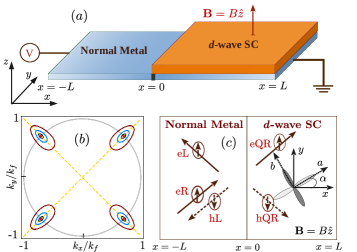
Figure 1: ($a$) Schematic diagram of normal metal/$d$-wave SC heterostructure with an externally applied Zeeman field $\mathbf{B}$ and voltage bias $V$. (b) The emergence of four BFSs with the Zeeman field $B=0.1$ (black), $0.2$ (blue), $0.5$ (brown). The normal state FS, four point nodes, and two line nodes are shown by the grey circle, red dots, and yellow dashed lines, respectively. (c) The scattering processes at the normal metal/$d$-wave SC junction is depicted where an incident up-spin ($\uparrow$) right-moving electron (eR) at the interface ($x$=0) can be scattered either as a normally reflected (left-moving) $\uparrow$ electron (eL) or Andreev reflected down-spin ($\downarrow$) hole hL, or transmitted as $\uparrow$ ($\downarrow$) electron (hole)-like quasiparticles eQR (hQR). Here, $\alpha$ is the angle between crystal $a$-axis and the interface normal.

In this letter, we propose to capture the signatures of BFSs in possible experimental observables based on normal metal/$d$-wave SC heterostructure. The coexistence of BQPs and Cooper pairs (CPs) in the BFS provides a rich playground for studying transport properties and the Fano factor (FF) characteristics in a simple setup. We show that topologically protected BFSs appear in the junction of normal metal/$d$-wave SC subjected to a perpendicular Zeeman field. Employing Blonder-Tinkham-Klapwijk (BTK) formalism, we calculate the differential conductance and find an enhancement in zero-bias conductance (ZBC), providing a key signature of BFSs. We extend our study to anisotropic $d$-wave SCs to explore the effect of anisotropy on BFSs. The emergence of zero-energy interface-localized Andreev bound states (ABS) is the previously established classic signature of anisotropy in $d$-wave SCs Hu (1994); Nagato and Nagai (1995); Tanaka and Tamura (2021); Tamura et al. (2017). The interplay between ABS and BFSs gives rise to intriguing features of ZBC for the anisotropic case. To confirm the role of BFSs in the anomalous behavior of the conductance, we perform a detailed analysis of shot-noise spectroscopy. We use both continuum and lattice model, and find a perfect match between the results obtained in the two models, establishing the robustness of the transport signatures of BFSs.

Model $\&$ topological BFSs- We consider a junction comprising of a normal metal and $d$-wave SC (N/SC) in presence of a Zeeman field (only in the SC side i.e. $x>0$) applied along $\hat{z}$ direction as shown in Fig. 1(a). We write the Bogoliubov-de Gennes (BdG) Hamiltonian: $H_{{\rm{BdG}}}=\frac{1}{2}\sum_{k}\Psi_{\mathbf{k}}^{\dagger}\mathcal{H}(\mathbf{k})\Psi_{\mathbf{k}}$ in Nambu basis as $\Psi_{\mathbf{k}}=[c_{\mathbf{k},\uparrow},c_{\mathbf{k},\downarrow},c^{\dagger}_{-\mathbf{k},\downarrow},-c^{\dagger}_{-\mathbf{k},\uparrow}]^{T}$, with $c_{\mathbf{k}\sigma}(c_{\mathbf{k}\sigma}^{\dagger})$ denotes annhilation (creation) operator for electrons with momentum $\mathbf{k}$ ($=\{k_{x},k_{y}\}$) and spin $\sigma$. We describe $\mathcal{H}(\mathbf{k})$ as  Setty et al. (2020a); Yang and Sondhi (1998),

$$\mathcal{H}(\mathbf{k})=\epsilon(\mathbf{k})\pi_{z}\sigma_{0}-B\pi_{0}\sigma_{z}+\Delta(\mathbf{k})\pi_{x}\sigma_{0}\ .$$ (1)

The Pauli matrices $\mathbf{\pi}$ and $\mathbf{\sigma}$ act on the particle-hole and spin degrees of freedom, respectively. The kinetic energy is given by: $\displaystyle{\epsilon(\mathbf{k})=\frac{\mathbf{k}^{2}}{2m}}-\mu$ where $m$ is the effective mass of electrons and $\mu$ is the chemical potential. Also, $B$ denotes the external Zeeman field. The superconductivity is induced via the proximity effect considering the pair potential as $\Delta(\mathbf{k})=\Delta_{0}\cos(2(\theta+\alpha))$ with $\theta=\tan^{-1}(k_{y}/k_{x})$ and $\alpha$ as the angle of anisotropy. Throughout our study, we consider natural unit, explicitly, $m=1$, $\Delta_{0}=1$, and set $\mu=10\Delta_{0}$, $\alpha=0$ (isotropic), and $\alpha=\pi/4$ (anisotropic). The external magnetic field only couples with the spin degree of freedom of electrons. The magnetic field strength is always taken less than the critical strength ($B=0.56\Delta_{0}$) Yang and Sondhi (1998). The change in other parameter values do not qualitatively affect the main message of the present work. Note that, $\Delta_{0}=0$ in the normal part of the junction ($x<0$).

In our model, when the Zeeman field is present in the $d$-wave SC side, four BFSs appear in the momentum space centred around $\mathbf{k}=(\pm k_{f},\pm k_{f})/\sqrt{2}$. They are illustrated by the zero-energy contours in Fig. 1(b). The area of each contour continuously increases as we enhance the strength of the Zeeman field. The topological property of BFSs can be identified by calculating the Pfaffian Agterberg et al. (2017a); Brydon et al. (2018). For the present model, it takes the form - $Pf(\mathbf{k})=\epsilon(\mathbf{k})^{2}+\Delta(\mathbf{k})^{2}-B^{2}$ as shown by Setty et al. Setty et al. (2020a), and $Pf(\mathbf{k})$ changes its sign accross each closed contour of BFS. To quantify it, a $\mathcal{Z}_{2}$ topological invariant, $\nu$, is defined as Agterberg et al. (2017a); Brydon et al. (2018): $(-1)^{\nu}=sgn[Pf(\mathbf{k})Pf(0)]$, where, $Pf(0)$ is computed at the origin in the momentum space. The closed contours of BFSs separate $\nu=0$ (outside) from the $\nu=1$ (inside) regions, indicating the topological protection of BFSs in our model. We refer to the supplementary material (SM) SM for more details on BFSs, and Pfaffian calculation.

With the understanding of the topological property of BFSs, we now focus on the four quantum mechanical scattering processes taking place at the N/SC junction as schematically shown in Fig. 1(c). A right-moving electron with spin $\sigma$ can (i) reflect as an electron with spin $\sigma$, called ordinary or normal reflection (NR), (ii) combine with another electron of opposite spin $\bar{\sigma}$ to form a spin-singlet CP leaving behind a hole to reflect from the interface due to the Andreev reflection (AR) process (for sub-gap energy), transmit as (iii) electron-like quasiparticle (QP) or (iv) hole-like QP. See the SM for detailed discussions SM .

Differential conductance- In order to find the signature(s) of BFSs, we calculate the differential conductance with the voltage bias $V$ applied across the junction using the BTK formula Blonder et al. (1982)

$$G(eV)=\frac{e^{2}}{h}\sum_{\sigma}\int_{-\pi/2}^{\pi/2}d\theta_{e}\cos\theta_{e}(1-\mathcal{R}^{e}_{\sigma}+\mathcal{R}^{h}_{\sigma})$$ (2)

where, $\mathcal{R}^{e}_{\sigma}=|r^{ee}_{\sigma}|^{2}$ ($\mathcal{R}^{h}_{\sigma}=\frac{\cos\theta_{h}}{\cos\theta_{e}}|r^{eh}_{\sigma}|^{2}$) denotes the probability with $r^{ee}_{\sigma}$ ($r^{eh}_{\sigma})$ being the amplitude for the NR (AR) from the interface, respectively. Also, $\theta_{e}$ ($\theta_{h}$) is the angle of incidence (reflection) of electron (hole). To compute the conductance, we numerically compute all possible scattering probabilities following the scattering matrix formalism (see SM for details SM ). According to the conservation of the probability current, the unitarity relation is always maintained: $\mathcal{R}^{e}_{\sigma}+\mathcal{R}^{h}_{\sigma}+\mathcal{T}^{e}_{\sigma}=1$ where $\mathcal{T}^{e}_{\sigma}$ is the probability of electron transmission, which can be finite within the subgap regime only in the presence of finite density of states (DOS) arising due to BFSs. The conductance in our N/SC junction is normalized by the normal metal conductance as $G_{N}=\frac{e^{2}}{h}\int_{-\pi/2}^{\pi/2}d\theta_{e}\cos\theta_{e}\frac{4\cos^{2}\theta_{e}}{4\cos^{2}\theta_{e}+Z^{2}}$, where $Z$ is the dimensionless barrier strength.

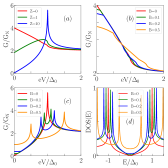
Figure 2: Normalized differential conductance is depicted as a function of voltage bias in ($a$) absence of Zeeman field ($B=0$), (b) transparent limit ($Z=0$), (c) tunneling limit ($Z=10$). (d) DOS of isotropic $d$-wave SC is shown in the presence of Zeeman field $B$.

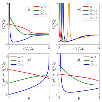
Figure 3: ($a$) Normalized differential conductance is shown as a function of voltage bias in (a) absence of Zeeman field ($B=0$), (b) tunneling limit ($Z=10$) for N/anisotropic $d$-wave SC junction. ZBC is depicted as a function of the magnetic field for the (c) isotropic and (d) anisotropic N/$d$-wave SC setup respectively.

In Fig. 2(a), we show the normalized differential conductance $G/G_{N}$ as a function of $eV$ in absence of any Zeeman field for the isotropic $d$-wave SC. In the transparent limit ($Z=0$), we find the decaying nature of the conductance for $eV<\Delta_{0}$ starting from the value $4$ (considering both spins) at zero energy (bias) and reach the saturation limit of $2$ for $eV>\Delta_{0}$. However, the behavior of the conductance qualitatively changes in the presence of a barrier. In the tunnelling limit ($Z\gg 0$), the conductance follows the quasiparticle DOS of the bulk $d$-wave SC with decreasing ZBC from $4$ to $0$ with increasing $Z$. This happens due to the enhancement of NR probability as $Z$ increases. We approximate Eq. (2) for the two transparency limits as: $G(eV,Z=0)\!=\!\frac{e^{2}}{h}\sum_{\sigma}\int_{-\pi/2}^{\pi/2}d\theta_{e}\cos\theta_{e}(1+\mathcal{R}^{h})\!=\!\frac{e^{2}}{h}\sum_{\sigma}\int_{-\pi/2}^{\,\pi/2}d\theta_{e}\cos\theta_{e}(2-\mathcal{T}^{e})$ and $G(eV,Z\gg 0)\!\sim\!\frac{e^{2}}{h}\sum_{\sigma}\int_{-\pi/2}^{\pi/2}d\theta_{e}\cos\theta_{e}(1-\mathcal{R}^{e})\!=\!\frac{e^{2}}{h}\sum_{\sigma}\int_{-\pi/2}^{\,\pi/2}d\theta_{e}\cos\theta_{e}\mathcal{T}^{e}$.

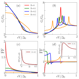
Figure 4: Normalized differential conductance is shown for the lattice model as a function of voltage bias in ($a$) transparent limit ($Z=0$), (b) tunneling limit ($Z=10$) considering the length and width of the lattice as $100a$ and $500a$ respectively, $a$ being the lattice spacing. (c) FF is illustrated as a function of $eV/\Delta_{0}$ choosing $Z=10$ for (c) $\alpha=0$ and (d) $\alpha=\pi/4$. Inset: ${\rm{FF}}~{}(eV=0)$ is highlighted as a function of the Zeeman field $B$. In panels (b), (c), and (d), different color lines indicate the same $B$ values as mentioned in panel (a).

Now, we turn on Zeeman field $B$ and depict the corresponding differential conductance in Figs. 2(b) and (c) for the two limits of $Z$. In the transparent limit ($Z=0$), we observe that almost flat region appears in the conductance profile and the magnitude of ZBC decreases as we increase $B$. However, when $eV>\Delta_{0}$, the behavior of appproaching the saturation limit is similar to the previous case. Decrease in conductance for $eV/\Delta_{0}<1$ means either reduction in the AR probability (see above equations) or equivalently, increase in the transmission since NR cannot take place in the fully transparent limit. However, transmission process can take place if the QP DOS is finite for $eV<\Delta_{0}$, which arises when BFSs accompanied by finite BQP DOS appear. The flat regions around $eV=0$ in the DOS gets elevated gradually with increasing $B$ as shown in Fig. 2(d). This clearly reflects in the decreasing behavior of the conductance in the transparent limit (see Fig.2(b)). On the other hand, in the tunneling limit ($Z\gg 0$), the conductance peak arising at $eV=\Delta_{0}$ splits into two and shifts to $eV_{\pm}=\Delta_{0}\pm B$, since the spin degeneracy is lifted as shown in Fig. 2(c). This splitting corresponds to the splitting we find in the DOS spectrum as depicted in Fig. 2(d). However, the enhancement of ZBC is due to the generation of BFSs as one increases B [see Fig. 2(c)]. Therefore, in both transparency limits, we find clear signatures of BFSs. In the literature, some attempts either incorporating disorder Oh et al. (2021) or Rashba spin-orbit interaction Banerjee et al. (2022), have been reported to find the signatures of BFSs. Disorder is always questionable in the context of identification. The latter one includes $s$-wave SCs Banerjee et al. (2022). Here, we show the clear signatures of BFSs in a N/$d$-wave SC junction for the first time which can be possible to realize using a conventional transport measurement setup, and thus enhances the importance of our work.

To address the issue of anisotropy $\alpha$, we show $G/G_{N}$ for $\alpha=\pi/4$ in Figs. 3(a) and (b). We choose this value of $\alpha$ in order to capture the maximum effect of the anisotropy. In the transparent limit, we find the differential conductance resembling the same as that of the isotropic SC [see Fig. 3(a)]. In contrast, in the tunneling limit, a ZBC peak develops due to the formation of the ABS. It is already established as a signature of the anisotropy in the literature Tanaka and Kashiwaya (1995). Interestingly, the ZBC peak is splitted and moves towards the higher $eV$ with increasing $B$ as shown in Fig. 3(b). To investigate the behavior of the conductance at $eV=0$ in more details, we show the ZBC as a function of $B$ for the isotropic and anisotropic $d$-wave SC in Figs. 3(c) and (d), respectively. For the isotropic SC, we observe a decrease in ZBC with the increase in $B$ in the transparent limit whereas, following the trend of increasing zero-energy DOS with $B$, ZBC rises with $B$ in the tunneling limit. This is due to the development of BFSs with $B$. However, in sharp contrast to the isotropic case, the ZBC for the anisotropic SC initially falls very fast, but later rises with the increase in $B$ in the tunneling limit. Additionally, the ZBC peak developed due to the presence of zero-energy ABS at the interface now splits into two at $E=\pm B$ forming nonzero-energy ABSs resulting in decrease in ZBC.

We strengthen our results obtained in the continuum model by computing the differential conductance using the python package KWANT Groth et al. (2014) based on a square lattice (see SM SM for details). We present the results for the isotropic case in Figs. 4(a)-(b), both in the transparent and tunnelling limit, which is in good agreement with our continuum model based results (Figs. 2(b)-(c)). Other results for the lattice model are shown and discussed in the SM SM .

Fano factor- In order to unravel the role of BFSs in the anomalies found above, we investigate the behavior of the FF. We predict that the interplay of the two carriers, CPs and BQPs, gives rise to the different intricate features in the conductance spectra. It can be emphasized by examining the nature of the charge carriers participating in the transport. The CPs contribute to the conductance via AR which dominates over other scattering processes in the transparent limit, whereas BQPs contribute via tunneling. Depending on their relative concentration at BFSs we obtain different results of the FF for different barrier strengths.

At zero temperature, the zero-frequency shot noise power for a N/SC junction can be obtained as, $\mathcal{S}(eV)\!=\!\int_{0}^{eV}dE~{}\mathcal{S}_{T}(E)$ with $\displaystyle{\mathcal{S}_{T}(E)\!=\!\frac{2e^{3}}{h}\int_{-\pi/2}^{\pi/2}d\theta\cos\theta~{}\mathcal{S}_{\theta}(E,\theta)}$ where $\displaystyle{\mathcal{S}_{\theta}(E,\theta)\!=\![R^{e}(1-R^{e})+R^{h}(1-R^{h})+2R^{e}R^{h}]}$ Anantram and Datta (1996); Blanter and Büttiker (2000); Tanaka et al. (2000); de Jong and Beenakker (1994); Kobayashi and Hashisaka (2021); Zhu and Ting (1999). The total current is given by, $\displaystyle{I(eV)=\int_{0}^{eV}dE~{}G(E)}$ and the FF is the ratio of shot noise power to current given by, $\displaystyle{{\rm{FF}}(eV)=\mathcal{S}(eV)/2eI(eV)}$.

We numerically compute the FF as a function of the bias for the isotropic (see Fig. 4(c)) and anisotropic SC (see Fig.4(d)) in the tunneling limit ($Z\gg 1$), and FF ($eV=0$) as a function of $B$ in the insets. For the isotropic SC, when $B=0$, we observe that FF($eV=0$) is 2 indicating the presence of only CPs at zero energy (see Fig. 4(c)) Tanaka et al. (2000); Zhu and Ting (1999). For $eV>0$, it decreases rapidly and approaches to $1$ due to the nodal lines of $d$-wave SC as established in the literature Tanaka et al. (2000). However, for $B\neq 0$, we observe a rapid decrease in the FF ($eV=0$) (see Fig.4(c) inset) due to the generation of BFSs. This indicates the increase in BQPs population inside BFSs which reduces the effective charge of the zero-energy current carriers. Interestingly, this FF ($eV=0$) extends for finite $eV$ giving rise to plateau-like regions in the FF profile confirming the emergence of BFSs (see Fig. 4(c)). On the other hand, for anisotropic SC, in the absence of any $B$, the FF ($eV=0$) is zero due to the presence of zero-energy ABS at $eV=0$ (Fig. 4(d)) Tanaka et al. (2000); Zhu and Ting (1999) which effectively suppresses the contribution of CPs, making their charge signatures undetectable. However, for $B\neq 0$, ABSs are formed at non-zero energies which manifest itself through sharp drops at $eV=B$ in the FF profile. In the FF ($eV=0$) behavior, there is a sharp rise of the FF followed by a gradual decrease with the increasing $B$ (see Fig. 4(d) inset). This initial sharp increase, reaching a value close to 2, indicates the presence of both CPs and BQPs for $B\neq 0$, which was previously undetectable due to the zero-energy ABS. As $B$ increases, more BQPs populate the BFSs, leading to a reduction in the effective charge of the zero-energy carriers, and thus resulting in a decrease in the FF ($eV=0$).

Having discussed the features of the FF, we finally address their connection to the behavior of the conductance discussed in the previous section. In the transparent limit ($Z=0$), where $G~{}(eV=0)$ is dominated by AR, when the Zeeman field is turned on, the relative concentration of BQPs increases inside BFSs, thus reducing the probability of the AR which further lowers the ZBC. Our results of the conductance for the anisotropic SC can be explained in a similar fashion. In the tunneling limit ($Z\gg 1$), AR is suppressed by NR due to the strong barrier potential and $G~{}(eV)$ effectively depends on the probability of QP transmission. Presence of BFSs increases zero energy DOS which enhances the QP transmission, and hence ZBC increases with $B$ for the isotropic case. For the anisotropic SC, ZBC initially falls sharply since zero-energy ABS shifts to non-zero energy along with a subsequent appearance of non-zero conductance peaks. As BFSs grow in size, more BQPs start populating which increases the tunneling probability, resulting in the enhancement of ZBC.

Concluding remarks- In this article, we propose that the differential conductance measurement at the interface between a normal metal and TRS-broken $d$-wave SC can reveal the signatures of topologically protected BFSs as zero-energy excitations. We have shown an enhancement in ZBC with $B$ as the key signature of BFSs in isotropic $d$-wave SC. On the contrary, the presence of ZBC peak due to the ABS formed at the interface has been found as an obstruction for the identification of the BFSs in anisotropic $d$-wave SC. We resolve this by applying the Zeeman field when the zero-energy ABS moves to nonzero-energy enabling the detection of BFSs at the zero-bias. For confirmation, we further reveal the anomalous behavior of the ZBC due to the interplay of BFS and ABS in noise spectroscopy by computing the FF. The simplicity of our setup, the availability of iron-based SCs (to serve as $d$-wave -SCs), and the clear signatures of BFSs found in it strengthens our proposal towards a compelling testbed for BFSs.

A. P. acknowledges Debmalya Chakraborty, Pritam Chaterjee, and Arnob Kumar Ghosh for stimulating discussions. P. D. acknowledges Department of Science and Technology (DST), India for the financial support through SERB Start-up Research Grant (File no. SRG/2022/001121).

In this supplementary material, we present more discussions on BFSs and the scattering matrix formalism in Sec. I and Sec. II respectively. Sec. III and Sec. IV are devoted to the discussion of our lattice model and some more results based on that to support the results presented in the main text.

Appendix A SI.  Bogoliubov Fermi Surfaces

In this section, we begin with the band structure and Fermi surfaces (FSs) of the four band continuum model introduced in the main text (see Eq. (1)) for both isotropic and anisotropic case and present them in Fig. S1 and Fig. S2, respectively. After diagonalizing the Hamiltonian, the energy eigenvalues are obtained as:

$$E_{\sigma,\eta}(\mathbf{k})=-\sigma B+\eta\sqrt{\epsilon(\mathbf{k})^{2}+\Delta(\mathbf{k})^{2}}\ .$$ (S1)

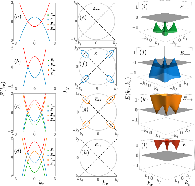
Figure S1: (a)-(d): Energy spectrum is depicted as a function of $k_{x}$ for the four band model of isotropic $d$-wave SC ($\alpha=0$) with $k_{y}=k_{f}/\sqrt{2}$ where we choose $(\Delta_{0},B)={(0,0),(1,0),(1,0.2\Delta_{0}),(1,0.5\Delta_{0})}$, respectively. (e)-(h): The Fermi surfaces for the four bands with $(\Delta_{0},B)=(1,0.5\Delta_{0})$ are illustrated. BFSs appear in $E_{--}$ and $E_{++}$. Here, the transparent circle represents the normal state FS. The dotted line denotes the nodal lines of $d$-wave SC. (i)-(l): Band structure in $k_{x}-k_{y}$ plane for $(\Delta_{0},B)=(1,0.5\Delta_{0})$ is demonstrated for better clarity. Only $E_{--}$ and $E_{++}$ intersect the zero energy plane (shown by grey color) hosting BFSs.

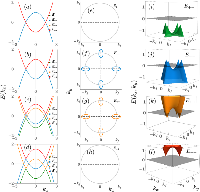
Figure S2: (a)-(d): Energy spectrum is shown as a function of $k_{x}$ for the four band model of anisotropic SC ($\alpha=\pi/4$) with $k_{y}=0$ where we choose $(\Delta_{0},B)={(0,0),(1,0),(1,0.2\Delta_{0}),(1,0.5\Delta_{0})}$, respectively. (e)-(h): Fermi surfaces for the same four bands with $(\Delta_{0},B)=(1,0.5\Delta_{0})$ are depicted. BFSs appear in $E_{--}$ and $E_{++}$ band. The transparent circle represents normal state FS. The dotted lines denote the nodal lines of $d$-wave SC. (i)-(l): The same band structures in $k_{x}-k_{y}$ plane for $(\Delta_{0},B)=(1,0.5\Delta_{0})$ are shown. Only $E_{--}$ and $E_{++}$ intersect the zero-energy plane (shown by grey color) hosting BFSs.

For the isotropic $d$-wave SC, we show the band structure of the four bands in Figs. S1(a)-(d) considering various values of $(\Delta_{0},B)$ by fixing $k_{y}$ at $k_{f}/\sqrt{2}$ where BFSs appear (the locations of the BFSs are mentioned in the main text). For zero Zeeman field ($B=0$) and SC gap ($\Delta_{0}=0$), the presence of the spin degeneracy leads to doubly degenerate bands in the system, denoted by $E_{++}$, $E_{-+}$, $E_{--}$ and $E_{+-}$. Here, $E_{++}$ and $E_{-+}$ (also $E_{--}$ and $E_{+-}$) overlap with each other as shown in Fig. S1(a). The conduction bands and valence bands touch each other at $k_{x}=\pm k_{f}\sqrt{2}$. With the introduction of the superconductivity, the degeneracy and the band touching phenomena remains the same because of the presence of nodal lines in $d$-wave SC (see Fig. S1(b)). When the Zeeman field is turned on, the spin degeneracy is lifted and the bands cross each other at multiple points (see Fig. S1(c-d)). In this scenario, increase in the Zeeman field results in the increase in the splitting of the bands.

In the absence of any superconductivity and Zeeman field, normal state FS for our four band model is a circle of radius $k_{f}=\sqrt{2m\mu}$. Introducing $d$-wave superconductivity gives rise to the four nodal lines positioned along $k_{x}=\pm k_{y}$. These four nodal lines intersect the normal state FS at four points, $(k_{x},k_{y})=(\pm k_{f}/\sqrt{2},\pm k_{f}/\sqrt{2})$ (see Fig. S1(e)). In the presence of $d$-wave SC, the normal state FS is gapped out leaving only these four points unaffected. Upon the introduction of a Zeeman field, these point nodes expand, giving rise to the formation of Bogoliubov Fermi surfaces (BFSs) as shown in the main text. However, all the four bands do not host BFSs. Only two bands $E_{++}$ and $E_{--}$ out of the four bands host four BFSs which is evident from Fig. S1(e-h). We also illustrate the appearance of BFSs in the $k_{x}-k_{y}$ plane for all four bands in Fig. S1(i-l) where only two bands $E_{--}$ and $E_{++}$ intersect the zero energy plane (see Fig. S1(j-k)) corroborating the emergence of BFSs as shown in Fig. S1(f-g). The area of intersection increases with the increase in $B$ as shown and mentioned in the main text.

For the anisotropic SC, the nodal lines of $d$-wave SC intersects the normal state FS at $(k_{x},~{}k_{y})=(0,\pm k_{f})$ and $(\pm k_{f},0)$ (see Fig. S2(e)). In Fig. S2 (a-d), we depict all the four bands as a function of $k_{x}$ with $k_{y}=0$ and the other parameter values are chosen as the same as isotropic SC. In the absence of any Zeeman field, the conduction and valence bands touch each other at $k_{x}=\pm k_{f}$. The Fermi surfaces and band structures in $k_{x}-k_{y}$ plane for the similar parameter values as for isotropic SC is depicted in Fig. S2(e-h) and Fig. S2(i-l), respectively. We observe that BFSs appears for the same bands as for the isotropic case but rotated by the angle of anisotropy i.e. $\alpha=\pi/4$. This occurs due to the rotation of the nodal lines of the $d$-wave SC.

In order to characterize the topological property of BFSs, we calculate the Pfaffian for the sake of completeness. Calculation of the Pfaffian relies on the fact that the Hamiltonian can be transformed into an antisymmetric matrix via a unitary transformation i.e. $\tilde{\mathcal{H}}(\mathbf{k})=\Omega\mathcal{H(\mathbf{k})}\Omega^{\dagger}$ so that $\tilde{\mathcal{H}}^{T}(\mathbf{k})=-\tilde{\mathcal{H}}(\mathbf{k})$ Agterberg et al. (2017a); Brydon et al. (2018). The Hamiltonian in Eq. (1) preserves both the charge conjugation ($\mathcal{C}$) and parity ($\mathcal{P}$) symmetry individually as well as their product ($\mathcal{CP}$), and thus satisfies the following relations:

$$\hat{\mathcal{C}}\mathcal{H}(\mathbf{k})\hat{\mathcal{C}}^{\dagger} = -\mathcal{H}(-\mathbf{k})\ ,$$ (S2)

$$\hat{\mathcal{P}}\mathcal{H}(\mathbf{k})\hat{\mathcal{P}}^{\dagger} = \mathcal{H}(-\mathbf{k})\ ,$$ (S3)

$$(\hat{\mathcal{C}}\hat{\mathcal{P}})\mathcal{H}(\mathbf{k})(\hat{\mathcal{C}}\hat{\mathcal{P}})^{\dagger} = -\mathcal{H}(\mathbf{k})\,.$$ (S4)

where $\hat{\mathcal{C}}=U_{C}\mathcal{K}=\pi_{y}\sigma_{0}\mathcal{K}$ and $\hat{\mathcal{P}}=U_{P}=\pi_{0}\sigma_{0}$ with $\mathcal{K}$ as complex conjugation operator. Using these expressions, we can rewrite the above relation as,

$$U_{CP}\mathcal{H}^{T}(\mathbf{k})U^{\dagger}_{CP}=-\mathcal{H}(\mathbf{k})$$ (S5)

where $U_{CP}=U_{C}U^{*}_{P}$. For the class of Hamiltonians satisfying this relation, one can construct a unitary matrix $\Omega$ which can transform $\mathcal{H}(\mathbf{k})$ into an antisymmetric form $\tilde{\mathcal{H}}(\mathbf{k})$. Thus, the Pfaffian $Pf(\mathbf{k})$, becomes well-defined and takes the form as, $Pf(\mathbf{k})=\epsilon(\mathbf{k})^{2}+\Delta(\mathbf{k})^{2}-B^{2}$ as mentioned in the main text Setty et al. (2020a). However, the existence of a well-defined Pfaffian, $Pf(\mathbf{k})$, does not imply the non-trivial topology of BFSs. For the topological protection of FSs, $Pf(\mathbf{k})$ must changes its sign over the momentum space. It can be shown that for any non-zero value of $B$, $Pf(\mathbf{k})$ changes sign in momentum space ensuring the emergence of tpological BFSs as mentioned in the main text.

Appendix B SII.  Scattering Matrix Formalism

Here, we discuss the details of our scattering matrix formulation to compute the differential conductance. We solve the following BdG Hamiltonian to find the quasiparticle excitations having energy $E$ measured with respect to $\mu$,

$$\begin{pmatrix}H_{N}({\mathbf{k}})-\mu&\Delta_{\mathbf{k}}\sigma_{0}\\ \Delta_{\mathbf{k}}\sigma_{0}&\mu-\mathcal{T}H_{N}(-\mathbf{k})\mathcal{T}^{-1}\\ \end{pmatrix}\begin{pmatrix}u\\ v\\ \end{pmatrix} =E\begin{pmatrix}u\\ v\\ \end{pmatrix}\ ,$$ (S6)

with $\displaystyle{\Delta_{\mathbf{k}}=\Delta(\theta)e^{i\phi}\Theta(x)}$ where $\Theta(x)$ is the Heavyside step function and $\phi$ is the global $U(1)$ phase of the SC. $\mathcal{T}=i\sigma_{y}\mathcal{K}$ is the time-reversal operator and $\mathcal{K}$ denotes the complex conjugation operator as mentioned in the previous section. Here, the Pauli matrix $\mathbf{\sigma}$ acts on the spin space. We consider the normal part Hamiltonian as mentioned in the main text where for the SC ($x>0$) a nonzero pair potential $\Delta(\mathbf{k})$ is introduced via the proximity-induced effect and it is zero for the normal metal (N) ($x<0$) side. Here, $u$ and $v$ are the two component spinors representing the electron and hole part of the QPs respectively. A thin insulating barrier with strength $V_{0}$ is modelled by a $\delta$-function potential at the interface ($x=0$) .

Solving the BdG equation for $x<0$ and $x>0$ separately, we obtain the scattering states as follows. In the normal side ($x<0$), the scattering states are given by,

$$\psi^{{\rm{inc}}}_{e,\uparrow}(x)=\begin{bmatrix}~{}1~{}\\ 0\\ 0\\ 0\end{bmatrix}e^{ik_{e}\cos\theta_{e}x}\ ,~{}~{}\psi^{{\rm{inc}}}_{e,\downarrow}(x)=\begin{bmatrix}~{}0~{}\\ 1\\ 0\\ 0\end{bmatrix}e^{ik_{e}\cos\theta_{e}x}\ ,$$

$$\psi^{{\rm{ref}}}_{e,\uparrow}(x)=\begin{bmatrix}~{}1~{}\\ 0\\ 0\\ 0\end{bmatrix}e^{-ik_{e}\cos\theta_{e}x}\ ,~{}~{}\psi^{{\rm{ref}}}_{e,\downarrow}(x)=\begin{bmatrix}~{}0~{}\\ 1\\ 0\\ 0\end{bmatrix}e^{-ik_{e}\cos\theta_{e}x}\ ,$$

$$\psi^{{\rm{ref}}}_{h,\downarrow}(x)=\begin{bmatrix}~{}0~{}\\ 0\\ 1\\ 0\end{bmatrix}e^{ik_{h}\cos\theta_{h}x}\ ,~{}~{}\psi^{{\rm{ref}}}_{h,\uparrow}(x)=\begin{bmatrix}~{}0~{}\\ 0\\ 0\\ 1\end{bmatrix}e^{ik_{h}\cos\theta_{h}x}\ ,$$

where $\psi^{{\rm{inc(ref)}}}_{\alpha,\sigma}(x)$ denotes the incident (reflected) state with spin $\sigma=\{\uparrow,\downarrow\}$, and $\alpha=\{e,h\}$ represents the electron and hole states, respectively. The momenta of the incident electron and reflected hole are given by respectively,

$$k_{e}=\sqrt{2m(E+\mu)}\ ,$$ (S7)

$$k_{h}=\sqrt{2m(E-\mu)}\ .$$ (S8)

The angle $\theta_{e}$ and $\theta_{h}$ correspond to the electron incident and hole reflection angle, respectively. Using the conservation of the parallel component of the momentum we write,

$$k_{e}\sin\theta_{e}=k_{h}\sin\theta_{h}\ ,$$ (S9)

where the expression for $\theta_{h}$ can be obtained as

$${\theta_{h}=\sin^{-1}\left(\sqrt{\frac{\mu+E}{\mu-E}}\sin\theta_{e}\right)}\ .$$ (S10)

This condition limits the possibility of Andreev reflection above a critical incident angle given by

$${\theta_{h}^{{\rm{critical}}}=\sin^{-1}\left(\sqrt{\frac{\mu+E}{\mu-E}}\right)}\ .$$ (S11)

The scattering states inside the SC ($x>0$) can be written as,

$$\psi^{{\rm{trans}}}_{eL,\uparrow}(x)=\begin{bmatrix}~{}u_{\uparrow}(\theta_{+})~{}\\ 0\\ v_{\uparrow}(\theta_{+})e^{-i\phi_{+}}\\ 0\end{bmatrix}e^{ik_{eL,\uparrow}x\cos\theta_{eL,\uparrow}}\ ,~{}~{}\psi^{{\rm{trans}}}_{eL,\downarrow}(x)=\begin{bmatrix}~{}0~{}\\ u_{\downarrow}(\theta_{+})\\ 0\\ v_{\downarrow}(\theta_{+})e^{-i\phi_{+}}\end{bmatrix}e^{ik_{eL,\downarrow}x\cos\theta_{eL,\downarrow}}\ ,$$

$$\psi^{{\rm{trans}}}_{hL,\uparrow}(x)=\begin{bmatrix}~{}v_{\uparrow}(\theta_{-})~{}\\ 0\\ u_{\uparrow}(\theta_{-})e^{-i\phi_{-}}\\ 0\end{bmatrix}e^{-ik_{hL,\uparrow}x\cos\theta_{hL,\uparrow}}\ ,~{}~{}\psi^{{\rm{trans}}}_{hL,\downarrow}(x)=\begin{bmatrix}~{}0~{}\\ v_{\downarrow}(\theta_{-})\\ 0\\ u_{\downarrow}(\theta_{-})e^{-i\phi_{-}}\end{bmatrix}e^{-ik_{hL,\downarrow}x\cos\theta_{hL,\downarrow}}\ ,$$

where $\psi^{{\rm{trans}}}_{eL(hL),\sigma}$ represents the transmitted electron-like (hole-like) quasi-particle state with spin $\sigma$. The momenta of the transmitted electron and hole like states with spin $\sigma$ are respectively given by,

$$k_{eL,\sigma}=\sqrt{2m(\mu+\sqrt{(E-\sigma B)^{2}-|\Delta(\theta_{+})|^{2}})}\ ,$$ (S12a)

$$k_{hL,\sigma}=\sqrt{2m(\mu-\sqrt{(E-\sigma B)^{2}-|\Delta(\theta_{-})|^{2}})}\ .$$ (S12b)

The superconducting coherence factors are given as follow:

$$\displaystyle{u_{\sigma}(\theta_{\pm})=\frac{1}{\sqrt{2}}\left[1+\sqrt{\frac{(E-\sigma B)^{2}-|\Delta(\theta_{\pm})|^{2}}{(E-\sigma B)^{2}}}\right]^{1/2}}\ ,$$ (S13a)

$$\displaystyle{v_{\sigma}(\theta_{\pm})=\frac{1}{\sqrt{2}}\left[1-\sqrt{\frac{(E-\sigma B)^{2}-|\Delta(\theta_{\pm})|^{2}}{(E-\sigma B)^{2}}}\right]^{1/2}}\ .$$ (S13b)

In the presence of anisotropy ($\alpha\neq 0$), the electron (hole)-like QPSs experience the pair potential as,

$$\Delta(\theta_{\pm})=\Delta_{0}\cos(2\theta\mp 2\alpha)\ ,$$ (S14)

satisfying the relation $\displaystyle{e^{i\phi_{\pm}}=e^{i\phi}\frac{\Delta(\theta_{\pm})}{|\Delta(\theta\pm)|}}$. The transmission angles for the electrons and holes inside the SC can be obtained employing the conservation of the $y$-component of wave-vector i.e.

$$k_{eL,\sigma}\sin\theta_{eL,\sigma} = k_{e}\sin\theta_{e}\ ,$$ (S15)

$$k_{hL,\sigma}\sin\theta_{hL,\sigma} = k_{e}\sin\theta_{e}\ ,$$ (S16)

where,

$$\displaystyle{\theta_{eL,\sigma}=\sin^{-1}\left(\sqrt{\frac{\mu+E}{\mu+\sqrt{(E-\sigma B)^{2}-|\Delta(\theta_{+})|^{2}}}}\sin\theta_{e}\right)}\ ,$$ (S17a)

$$\displaystyle{\theta_{hL,\sigma}=\sin^{-1}\left(\sqrt{\frac{\mu+E}{\mu-\sqrt{(E-\sigma B)^{2}-|\Delta(\theta_{-})|^{2}}}}\sin\theta_{e}\right)}\ .$$ (S17b)

Having the scattering states in both sides of the interface, we can write the wave functions in these two regions as,

$$\Psi^{N}_{\sigma}(x) = \psi^{{\rm{inc}}}_{e,\sigma}+r^{ee}_{\sigma}\psi^{{\rm{ref}}}_{e,\sigma}+r^{eh}_{\bar{\sigma}}\psi^{{\rm{ref}}}_{h,\bar{\sigma}}\ ,$$ (S18)

$$\Psi^{SC}_{\sigma}(x) = t^{ee}_{\sigma}\psi^{{\rm{trans}}}_{eL,\sigma}+t^{eh}_{\sigma}\psi^{{\rm{trans}}}_{hL,\sigma}\ ,$$ (S19)

where $r^{ee}_{\sigma},r^{eh}_{\sigma},t^{ee}_{\sigma},t^{eh}_{\sigma}$ denote the scattering amplitudes for the NR, AR, electron-like, and hole-like transmission, respectively. We obtain these amplitudes using boundary conditions given by,

$$\Psi^{N}_{\sigma}(x=0) =\Psi^{SC}_{\sigma}(x=0)\ ,$$ (S20a)

$$\frac{d}{dx}\Psi^{SC}_{\sigma}(x)\vline_{{}_{x=0^{+}}}-\frac{d}{dx}\Psi^{N}_{\sigma}(x)\vline_{{}_{x=0^{-}}} =Z\Psi^{N}_{\sigma}(x=0)\ .$$ (S20b)

Here, $Z=\frac{2mV_{0}}{\hbar^{2}k_{f}}$ is the dimensionless barrier strength. We numerically solve for $r^{ee}_{\sigma},r^{eh}_{\bar{\sigma}},t^{ee}_{\sigma},t^{eh}_{\sigma}$ using Eqs. (S20a) $\&$ (S20b) to compute the differential conductance and shot-noise spectra within the BTK formalism.

Appendix C SIII.  Lattice Model

In this section, we construct the lattice model starting from the continuum model introduced in the main text. We choose a square lattice with the lattice spacing $a=1$. The lattice Hamiltonian can be found by replacing $k_{i}^{2}\simeq 2(1-\cos k_{i}),k_{i}\simeq\sin k_{i}$ where $i=x,y$ as,

$$\mathcal{H}_{{\rm{lat}}}(\mathbf{k})=[-2t(\cos k_{x}+\cos k_{y})+(4t-\mu)]\pi_{z}\sigma_{0}-B\pi_{0}\sigma_{z}+\Delta_{{\rm{lat}}}(\mathbf{k},\alpha)\pi_{x}\sigma_{0}$$ (S21)

where, $\Delta_{{\rm{lat}}}(\mathbf{k},\alpha=0)=2\Delta_{0}(\cos k_{y}-\cos k_{x})$ and $\Delta_{{\rm{lat}}}(\mathbf{k},\alpha=\pi/4)=2\Delta_{0}\sin k_{x}\sin k_{y}$. We illustrate schematically the $d$-wave pair potential in the real space on a square lattice schematically for both the isotropic (see Fig. S3(a)) and anisotropic case (see Fig.S3(b)). For the isotropic $d$-wave SC ($\alpha=0$), the pairing happens between two nearest-neighbour sites with opposite spins whereas, in the anisotropic $d$-wave SC ($\alpha=\pi/4$), the pairing is considered between the next-nearest-neighbours with opposite spins.

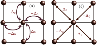
Figure S3: Schematic diagram of our lattice model with the $d$-wave pair amplitudes in the real space. (a) For isotropic SC, two nearest-neighbour electrons with opposite spins are paired (denoted by the curved arrows), whereas (b) for anisotropic SC, two next-nearest-neighbour electrons are paired (indicated by the straight arrows).

Appendix D SIV.  Differential conductance in case of lattice model

We also compute the normalized differential conductance for the lattice model using the python package KWANT Groth et al. (2014). In the main text, the differential conductance for the N/isotropic $d$-wave SC hybrid junction is presented based on our lattice model. Here, we show the normalized differential conductance considering the lattice model for the N/anisotropic $d$-wave SC setup for both the transperant (ballistic) and tunneling limit in Fig. S4(a) and Fig. S4(b), respectively. For this purpose, we consider a square lattice with dimension $N_{x}\times N_{y}$ and attach leads along $x$-direction at $x=\pm N_{x}$. The leads are modelled using the same Hamiltonian mentioned in Eq. (S21) with $B=0,~{}\Delta_{0}=0$. We choose the following parameters: $t=1,\mu=t,\Delta_{0}=0.01\mu,N_{x}=100a,Ny=350a$ ($a=1$) where $B$ is measured in units of $\Delta_{0}$. We find a fantastic agreement (in both transperant and tunneling limit) with the results obtained in case of continuum model for the same set of parameter values. This agreement enhances the potential of our work.

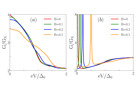
Figure S4: Normalized differential conductance is depicted considering the lattice model of N/anisotropic $d$-wave SC junction, as a function of the voltage bias for various values of the Zeeman field $B$ in the (a) ballistic ($Z=0$) and (b) tunneling ($Z=10$) limit.

References

- Bardeen et al. (1957) J. Bardeen, L. N. Cooper, and J. R. Schrieffer, Phys. Rev. 108, 1175 (1957).
- Sigrist and Ueda (1991) M. Sigrist and K. Ueda, Rev. Mod. Phys. 63, 239 (1991).
- Agterberg et al. (2017a) D. F. Agterberg, P. M. R. Brydon, and C. Timm, Phys. Rev. Lett. 118, 127001 (2017a).
- Brydon et al. (2018) P. M. R. Brydon, D. F. Agterberg, H. Menke, and C. Timm, Phys. Rev. B 98, 224509 (2018).
- Menke et al. (2019) H. Menke, C. Timm, and P. M. R. Brydon, Phys. Rev. B 100, 224505 (2019).
- Sumita et al. (2019) S. Sumita, T. Nomoto, K. Shiozaki, and Y. Yanase, Phys. Rev. B 99, 134513 (2019).
- Lapp et al. (2020) C. J. Lapp, G. Börner, and C. Timm, Phys. Rev. B 101, 024505 (2020).
- Tamura et al. (2020) S.-T. Tamura, S. Iimura, and S. Hoshino, Phys. Rev. B 102, 024505 (2020).
- Oh et al. (2021) H. Oh, D. F. Agterberg, and E.-G. Moon, Phys. Rev. Lett. 127, 257002 (2021).
- Kim et al. (2021) D. Kim, S. Kobayashi, and Y. Asano, Journal of the Physical Society of Japan 90, 104708 (2021).
- Dutta et al. (2021) P. Dutta, F. Parhizgar, and A. M. Black-Schaffer, Phys. Rev. Res. 3, 033255 (2021).
- Zhu et al. (2021) Z. Zhu, M. Papaj, X.-A. Nie, H.-K. Xu, Y.-S. Gu, X. Yang, D. Guan, S. Wang, Y. Li, C. Liu, J. Luo, Z.-A. Xu, H. Zheng, L. Fu, and J.-F. Jia, Science 374, 1381 (2021).
- Bhattacharya and Timm (2023) A. Bhattacharya and C. Timm, arXiv:2301.10524 (2023), 10.48550/arXiv.2301.10524.
- Miki et al. (2023) T. Miki, H. Ikeda, and S. Hoshino, arXiv:2304.04533 (2023), 10.48550/arXiv.2304.04533.
- Timm and Bhattacharya (2021) C. Timm and A. Bhattacharya, Phys. Rev. B 104, 094529 (2021).
- Bzdušek and Sigrist (2017) T. c. v. Bzdušek and M. Sigrist, Phys. Rev. B 96, 155105 (2017).
- Timm et al. (2021) C. Timm, P. M. R. Brydon, and D. F. Agterberg, Phys. Rev. B 103, 024521 (2021).
- Timm et al. (2017) C. Timm, A. P. Schnyder, D. F. Agterberg, and P. M. R. Brydon, Phys. Rev. B 96, 094526 (2017).
- Link and Herbut (2020) J. M. Link and I. F. Herbut, Phys. Rev. Lett. 125, 237004 (2020).
- Herbut and Link (2021) I. F. Herbut and J. M. Link, Phys. Rev. B 103, 144517 (2021).
- Oh and Moon (2020) H. Oh and E.-G. Moon, Phys. Rev. B 102, 020501 (2020).
- Link et al. (2020) J. M. Link, I. Boettcher, and I. F. Herbut, Phys. Rev. B 101, 184503 (2020).
- Setty et al. (2020a) C. Setty, Y. Cao, A. Kreisel, S. Bhattacharyya, and P. J. Hirschfeld, Phys. Rev. B 102, 064504 (2020a).
- Cao et al. (2023) Y. Cao, C. Setty, L. Fanfarillo, A. Kreisel, and P. Hirschfeld, arXiv preprint arXiv:2305.15569 (2023), 10.48550/arXiv.2305.15569.
- Banerjee et al. (2022) S. Banerjee, S. Ikegaya, and A. P. Schnyder, Phys. Rev. Res. 4, L042049 (2022).
- Setty et al. (2020b) C. Setty, S. Bhattacharyya, Y. Cao, A. Kreisel, and P. J. Hirschfeld, Nature Communications 11, 523 (2020b).
- Fulde (1965) P. Fulde, Phys. Rev. 137, A783 (1965).
- Gao et al. (2010) Y. Gao, W.-P. Su, and J.-X. Zhu, Phys. Rev. B 81, 104504 (2010).
- Nicholson et al. (2012) A. Nicholson, W. Ge, J. Riera, M. Daghofer, A. Moreo, and E. Dagotto, Phys. Rev. B 85, 024532 (2012).
- Nourafkan et al. (2016) R. Nourafkan, G. Kotliar, and A.-M. S. Tremblay, Phys. Rev. Lett. 117, 137001 (2016).
- Ong et al. (2016) T. Ong, P. Coleman, and J. Schmalian, Proceedings of the National Academy of Sciences 113, 5486 (2016).
- Nica et al. (2017) E. M. Nica, R. Yu, and Q. Si, npj Quantum Materials 2, 24 (2017).
- Chubukov et al. (2016) A. V. Chubukov, O. Vafek, and R. M. Fernandes, Phys. Rev. B 94, 174518 (2016).
- Agterberg et al. (2017b) D. F. Agterberg, T. Shishidou, J. O’Halloran, P. M. R. Brydon, and M. Weinert, Phys. Rev. Lett. 119, 267001 (2017b).
- Brydon et al. (2016) P. M. R. Brydon, L. Wang, M. Weinert, and D. F. Agterberg, Phys. Rev. Lett. 116, 177001 (2016).
- Yang et al. (2017) W. Yang, T. Xiang, and C. Wu, Phys. Rev. B 96, 144514 (2017).
- Roy et al. (2019) B. Roy, S. A. A. Ghorashi, M. S. Foster, and A. H. Nevidomskyy, Phys. Rev. B 99, 054505 (2019).
- Yu and Liu (2018) J. Yu and C.-X. Liu, Phys. Rev. B 98, 104514 (2018).
- Boettcher and Herbut (2018) I. Boettcher and I. F. Herbut, Phys. Rev. Lett. 120, 057002 (2018).
- Venderbos et al. (2018) J. W. F. Venderbos, L. Savary, J. Ruhman, P. A. Lee, and L. Fu, Phys. Rev. X 8, 011029 (2018).
- Kim et al. (2018) H. Kim, K. Wang, Y. Nakajima, R. Hu, S. Ziemak, P. Syers, L. Wang, H. Hodovanets, J. D. Denlinger, P. M. R. Brydon, D. F. Agterberg, M. A. Tanatar, R. Prozorov, and J. Paglione, Science Advances 4, eaao4513 (2018).
- Wang et al. (2018) Q.-Z. Wang, J. Yu, and C.-X. Liu, Phys. Rev. B 97, 224507 (2018).
- Schemm et al. (2014) E. R. Schemm, W. J. Gannon, C. M. Wishne, W. P. Halperin, and A. Kapitulnik, Science 345, 190 (2014).
- Luke et al. (1993) G. M. Luke, A. Keren, L. P. Le, W. D. Wu, Y. J. Uemura, D. A. Bonn, L. Taillefer, and J. D. Garrett, Phys. Rev. Lett. 71, 1466 (1993).
- Cao et al. (2018a) Y. Cao, V. Fatemi, A. Demir, S. Fang, S. L. Tomarken, J. Y. Luo, J. D. Sanchez-Yamagishi, K. Watanabe, T. Taniguchi, E. Kaxiras, R. C. Ashoori, and P. Jarillo-Herrero, Nature 556, 80 (2018a).
- Cao et al. (2018b) Y. Cao, V. Fatemi, S. Fang, K. Watanabe, T. Taniguchi, E. Kaxiras, and P. Jarillo-Herrero, Nature 556, 43 (2018b).
- Phan et al. (2022) D. Phan, J. Senior, A. Ghazaryan, M. Hatefipour, W. M. Strickland, J. Shabani, M. Serbyn, and A. P. Higginbotham, Phys. Rev. Lett. 128, 107701 (2022).
- Yang and Sondhi (1998) K. Yang and S. L. Sondhi, Phys. Rev. B 57, 8566 (1998).
- Christos and Sachdev (2023) M. Christos and S. Sachdev, arXiv:2308.03835 (2023).
- Hu (1994) C.-R. Hu, Phys. Rev. Lett. 72, 1526 (1994).
- Nagato and Nagai (1995) Y. Nagato and K. Nagai, Phys. Rev. B 51, 16254 (1995).
- Tanaka and Tamura (2021) Y. Tanaka and S. Tamura, Journal of Superconductivity and Novel Magnetism 34, 1 (2021).
- Tamura et al. (2017) S. Tamura, S. Kobayashi, L. Bo, and Y. Tanaka, Phys. Rev. B 95, 104511 (2017).
- (54) See Supplemental Material for details of the BFSs, Pfaffian calculation, scattering matrix formalism, Hamiltonian and results for the lattice model.
- Blonder et al. (1982) G. E. Blonder, M. Tinkham, and T. M. Klapwijk, Phys. Rev. B 25, 4515 (1982).
- Tanaka and Kashiwaya (1995) Y. Tanaka and S. Kashiwaya, Phys. Rev. Lett. 74, 3451 (1995).
- Groth et al. (2014) C. W. Groth, M. Wimmer, A. R. Akhmerov, and X. Waintal, New Journal of Physics 16, 063065 (2014).
- Anantram and Datta (1996) M. P. Anantram and S. Datta, Phys. Rev. B 53, 16390 (1996).
- Blanter and Büttiker (2000) Y. Blanter and M. Büttiker, Physics Reports 336, 1 (2000).
- Tanaka et al. (2000) Y. Tanaka, T. Asai, N. Yoshida, J. Inoue, and S. Kashiwaya, Phys. Rev. B 61, R11902 (2000).
- de Jong and Beenakker (1994) M. J. M. de Jong and C. W. J. Beenakker, Phys. Rev. B 49, 16070 (1994).
- Kobayashi and Hashisaka (2021) K. Kobayashi and M. Hashisaka, Journal of the Physical Society of Japan 90, 102001 (2021).
- Zhu and Ting (1999) J.-X. Zhu and C. S. Ting, Phys. Rev. B 59, R14165 (1999).
Supplementary Material for “Transport signatures of Bogoliubov Fermi surfaces in normal metal/-wave superconductor junctions”
Amartya Pal1,2, Arijit Saha
1,2 and Paramita Dutta
3
1Institute of Physics, Sachivalaya Marg, Bhubaneswar-751005, India
2Homi Bhabha National Institute, Training School Complex, Anushakti Nagar, Mumbai 400094, India
3Theoretical Physics Division, Physical Research Laboratory, Navrangpura, Ahmedabad-380009, India