Classical Non-Relativistic Fractons

Abstract

We initiate the study of the classical mechanics of non-relativistic fractons in its simplest setting - that of identical one dimensional particles with local Hamiltonians characterized by by a conserved dipole moment in addition to the usual symmetries of space and time translation invariance. We introduce a family of models and study the $N$ body problem for them. We find that locality leads to a “Machian” dynamics in which a given particle exhibits finite inertia only if within a specified distance of at least another one. For well separated particles this leads to immobility, much as for quantum models of fractons discussed before. For two or more particles within inertial reach of each other at the start of motion we get an interesting interplay of inertia and interactions. Specifically for a solvable “inertia only” model of fractons we find that $N=2$ particles always become immobile at long times. Remarkably $N=3$ particles generically evolve to a late time state with one immobile particle and two that oscillate about a common center of mass with generalizations of such “Machian clusters” for $N>3$ . Interestingly, Machian clusters exhibit physical limit cycles in a Hamiltonian system even though mathematical limit cycles are forbidden by Liouville’s theorem.

I Introduction and summary of main results

Much recent work in quantum many body theory has focused on the properties of so-called “fracton” or “fractonic” phases of matter. These phases [1, 2] host excitations with restricted mobility of which the ones which are immobile in isolation are termed fractons. This term in the current context is a legacy of the paper that kicked off the boom in which Haah discovered an exceptionally complicated example [3] wherein the operators that create widely separated fractons are fractal in character. Subsequently it was realized the basic phenomenon of immobility did not require fractality but could be done with simpler membrane operators and indeed had been done by Chamon much before [5]. A second important simplification was the realization that full blown fractons could be obtained by gauging models with unusual symmetries which already exhibited restricted particle mobility. The simplest such ungauged models exhibit the conservation of higher moments of the charge distribution i.e. multipoles [6, 7] and recent work has explored the effects of multipole conservation in continuum and and many-body quantum mechanical settings [7, 8, 9, 10].

In this work, we initiate the study of classical, non-relativistic, systems of point particles with multipole symmetries in the continuum. We do this by studying the simplest setting of systems with a conserved dipole moment in $d=1$ spatial dimensions. For such systems we study Hamiltonian mechanics for fixed numbers of point particles.

Even in this simple setting, we find many surprises that defy conventional intuition about classical particle systems. Overall we find that symmetry and locality conspire to produce a variant of Machian dynamics [11, 12, 13, 8] wherein particles exhibit inertia only in the presence of others and are motionless in isolation. The nature of dynamics exhibited by Machian clusters depends on $N$, the number of particles in close proximity, in addition to the nature of the Hamiltonian and initial conditions. In the absence of any additional particle interactions, $N=2$ particles in close initial separation generically separate and become immobile with the passage of time. $N=3$ particles generically settle down to a steady state dynamics in position space where one particle becomes immobile and the other two oscillate about a centre of mass in the manner of a limit cycle, seemingly violating (but ultimately consistent with) Liouville’s theorem. An exact solution for $N=3$ particles is obtained in an idealized limit. For $N=4$ and more, numerical integration of the equations of motion results in the particles separating into at least two clusters with the latter exhibiting motionless, oscillatory or chaotic dynamics at late times. Other unusual features that characterize the trajectories are (i) the breakdown of the customary relationships between momenta, velocity and energy, (ii) constant energy phase-space hypersurfaces that are unbounded in the momenta, (iii) the appearance of asymptotic, emergent, conserved quantities. Throughout the paper, we will refer to dipole conserving particles as ‘fractons’ which is now standard practice [14, 15, 16].

The paper is organized as follows. In Section II, we review how symmetries are implemented in classical Hamiltonian systems and write down the form of Hamiltonians compatible with dipole symmetry. In Section III, we numerically study the classical trajectories of $N=1,2,3,4$ fractons and in Section V, we obtain the exact solution for trajectories for $N=2,3$ for a specific form of the Hamiltonian. In Section VI, we discuss specific aspects of fracton trajectories and the parallels with known quantum fracton phenomenology in Section VII before concluding.

II Symmetries and compatible Hamiltonians

II.1 Symmetries in classical non-relativistic systems of point-particles

Consider a system of $N$ point particles living in $d$ spatial dimensions. We will work within the Hamiltonian framework to describe its dynamics. Here, the state of the system is specified by $2dN$ phase space coordinates consisting of $dN$ positions $\{x^{\mu}_{1},\ldots,x^{\mu}_{N}\}$ and $dN$ momenta $\{p^{\mu}_{1}\ldots p^{\mu}_{N}\}$. Dynamics is generated by the Hamiltonian $H(\{x^{\mu}_{a},p^{\mu}_{a}\})$ which gives us Hamilton’s equations of motion,

$$\dot{x}^{\mu}_{a}=\frac{\partial H}{\partial p^{\mu}_{a}},~{}\dot{p}^{\mu}_{a}=-\frac{\partial H}{\partial x^{\mu}_{a}}.$$ (1)

Above and henceforth, we will use the short hand notation $\dot{A}\equiv\frac{\partial A}{\partial t}$, the superscripts $\mu=1,\ldots,d$ to denote the spatial components of the phase space coordinates and subscripts $a=1,\ldots,N$ to specify the particle. We will also sometimes vectorize the spatial components of phase-space coordinates as $\vec{x}_{a},~{}\vec{p}_{a}$ etc.

Our main interest is to understand how Hamiltonian dynamics is constrained by dipole symmetries. As a warm up, let begin understanding the conservation of total charge. If the $N$ particles carry electric charges $\{q_{1},\ldots,q_{N}\}$ respectively, we can define the charge density $\rho$ and current $\vec{j}$ in the usual way

$$\rho(x) \equiv\sum_{a=1}^{N}q_{a}\delta^{d}(\vec{x}_{a}-\vec{x}),$$ (2)

$$\vec{j}(x) \equiv\sum_{a=1}^{N}q_{a}\dot{\vec{x}}_{a}\delta^{d}(\vec{x}_{a}-\vec{x}).$$ (3)

$\rho$ and $\vec{j}$ satisfy the continuity equation

$$\dot{\rho}+\vec{\nabla}.\vec{j}=0,$$ (4)

leading to the conservation of total charge $Q$

$$\dot{Q}=0~{}\text{ where, }Q\equiv\int d^{d}x~{}\rho(x)=\sum_{a}q_{a}.$$ (5)

Note that this conservation is a kinematic constraint and is built into the kinematic framework of classical non-relativistic Hamiltonian dynamics since the number of particles $N$ is fixed and cannot change. Consequently,  Eqs. 4 and 5 hold irrespective of the Hamiltonian form. This is not true of other symmetries which constrain the form of the Hamiltonian. For example, if we want to impose translation symmetry generated by

$$x^{\mu}_{a}\mapsto x^{\mu}_{a}+\xi^{\mu},~{}p^{\mu}_{a}\mapsto p^{\mu}_{a},$$ (6)

the form of the Hamiltonian is constrained to be

$$H(x^{\mu}_{a},p^{\mu}_{a})\equiv H\left(x^{\mu}_{a}-x^{\mu}_{b},p^{\mu}_{a}\right)$$ (7)

and leads to the conservation of the total momentum

$$\dot{P}^{\mu}=0,\text{where }~{}P^{\mu}\equiv\sum_{a=1}^{N}p^{\mu}_{a}.$$ (8)

We now turn to the main interest of this work and look to impose the conservation of the total dipole moment,

$$\dot{D}^{\mu}=0,~{}D^{\mu} \equiv\int d^{d}x~{}x^{\mu}\rho(x)=\sum_{a=1}^{N}q_{a}x^{\mu}_{a}$$ (9)

which induces the following symmetry transformation on the phase space coordinates

$$x^{\mu}_{a}\mapsto x^{\mu}_{a},~{}p^{\mu}_{a}\mapsto p^{\mu}_{a}+q_{a}\phi^{\mu}.$$ (10)

Comparing Eqs. 6 and 10, we see that dipole conservation implies translation in momentum space! This constrains the Hamiltonian to be of the form

$$H(x^{\mu}_{a},p^{\mu}_{a})\equiv H\left(x^{\mu}_{a},\frac{p^{\mu}_{a}}{q_{a}}-\frac{p^{\mu}_{b}}{q_{b}}\right).$$ (11)

This can easily be further generalized. While $Q$, shown in Eq. 5 is the zeroth moment of charge distribution, $\vec{D}$ shown in Eq. 9s is the first moment. We can further consider the conservation of arbitrary combinations of charge moments such as

$$\dot{M}_{P}=0,M_{P}=\int d^{d}x~{}P(x)\rho(x)=\sum_{a}q_{a}P(x_{a})$$ (12)

where $P(x)$ is some polynomial of the $d$ components $x^{\mu}$. This induces a so-called ‘polynomial shift’ symmetry

$$x^{\mu}_{a}\mapsto x^{\mu}_{a},~{}p^{\mu}_{a}\mapsto p^{\mu}_{a}+q_{a}\lambda\frac{\partial P(x_{a})}{\partial x^{\mu}_{a}}.$$ (13)

and generates the so-called multipole algebra discussed in Ref. [7] of which Eq. 10 is a special case. Symmetry compatible Hamiltonians which obey Eq. 13 are constrained to take the form

$$H\rightarrow H\left(\frac{p^{\mu}_{a}}{q_{a}}\left(\frac{\partial P(x_{a})}{\partial x^{\mu}_{a}}\right)^{-1}-\frac{p^{\mu}_{b}}{q_{b}}\left(\frac{\partial P(x_{b})}{\partial x^{\mu}_{b}}\right)^{-1}\right).$$ (14)

Note that the repeated indices are not summed over in the above equation. For the rest of this paper, we will restrict ourselves to dipole conservation symmetry shown in Eq. 9 and study the dynamics generated by Hamiltonians of the form Eq. 9 and leave the more general case of Eq. 13 for future work.

II.2 Symmetry compatible Hamiltonians

We now focus on the dipole conservation symmetry of Eqs. 9 and 10 and look at the possible forms the Hamiltonian of Eq. 11 can take. Recall that translation invariance of coordinates shown in Eq. 6 results in the Hamiltonian depending only on the difference of the coordinates as shown in Eq. 7. A common form of such a Hamiltonian is

$$H=\sum_{a}\frac{|\vec{p}_{a}|^{2}}{2m_{a}}+\sum_{a<b}U(x_{a}-x_{b})+\ldots$$ (15)

In order to be physically reasonable, we require the Hamiltonian be local i.e. particles with large distances $|\vec{x}_{a}-\vec{x}_{b}|$ between them should not affect each others dynamics. This requires the two-particle interaction in Eq. 15, represented by $U(x)$ to vanish as $|x|\rightarrow\infty$. Also, the quadratic form of the kinetic term, $|\vec{p}_{a}|^{2}$ ensures that energies are bounded from below. Let us now move on to the case of a Hamiltonian with dipole symmetry which has a functional form shown in Eq. 11. A natural modification of Eq. 15 to accommodate this is

$$H=\sum_{a<b}\left(\frac{1}{2m_{ab}}\left|\frac{\vec{p}_{a}}{q_{a}}-\frac{\vec{p}_{b}}{q_{b}}\right|^{2}+U(x_{a}-x_{b})+\ldots\right)$$ (16)

However, note that the leading momentum-dependent kinetic term is no longer local. To restore locality, we modify it as follows

$$H=\sum_{a<b}\left(\frac{K(|\vec{x}_{a}-\vec{x}_{b}|)}{2m_{ab}}\left|\frac{\vec{p}_{a}}{q_{a}}-\frac{\vec{p}_{b}}{q_{b}}\right|^{2}+U(x_{a}-x_{b})+\ldots\right)$$ (17)

where $K(x)$ is some function with local support that vanishes as $|x|\rightarrow\infty$ to impose locality. For the energies to be bounded from below, $K(x)$ should also be positive definite.

II.3 Mach’s principle

Figure 1: Sample particle configuration in d=2 corresponding to four visible Machian clusters. The dark red circles represent particles and the shaded blue region surrounding them represent the range where $K\neq 0$.

The unusual form of the kinetic term in Eq. 17 has several consequences which we will explore in the upcoming sections. Let us point out one of them here – the familiar relation between momentum and velocity – $\dot{x}_{a}\propto p_{a}$ no longer holds for Eq. 17. Instead, we have

$$\dot{x}^{\mu}_{a}=\frac{\partial H}{\partial p^{\mu}_{a}}=\sum_{b}\left(\frac{p^{\mu}_{a}}{q_{a}}-\frac{p^{\mu}_{b}}{q_{b}}\right)\frac{K(|x^{\mu}_{a}-x^{\mu}_{b}|)}{q_{a}m_{ab}}.$$ (18)

It is nice to see how dipole conservation works out from the form of the velocities in Eq. 18:

$$\dot{D}^{\mu}=\sum_{a}q_{a}\dot{x}^{\mu}_{a}=\sum_{a,b}\left(\frac{p^{\mu}_{a}}{q_{a}}-\frac{p^{\mu}_{b}}{q_{b}}\right)\frac{K(|x^{\mu}_{a}-x^{\mu}_{b}|)}{m_{ab}}=0.$$ (19)

Equation 18 tells us that the velocity of a given particle is affected by all others. This is reminiscent of Mach’s principle [11] which states that motion of a body is not absolute but is influenced by all others in the cluster. In the context of gravity where this principle has been most discussed [12, 13], the formulation aims to describe the motion of particles within a single cluster and is inherently non-local. For instance, the kinetic term in Ref. [17] is similar to the one shown in Eq. 16. The inclusion of the locality term $K(x)$ which is natural in the context of condensed matter physics changes the picture qualitatively. Here, the motion of a particle, located at position $\vec{x}_{a}$ is influenced, not by all particles, but only those particles located at $\vec{x}_{b}$ such that $K(\vec{x}_{a}-\vec{x}_{b})\neq 0$. The dynamics of Eq. 17 is therefore that of particles living in and moving between multiple dynamical clusters as shown in Fig. 1. We use the term ‘Machian cluster’ to refer to a collection of particles which lend inertia and facilitate each others motion. Notice that the number of Machian clusters can change under dynamics as particles move apart or come together. The connection between dipole conserving systems and Mach’s principle was originally pointed out in Ref. [6] using a continuum field theoretic formulation, for quantum systems. Our non-relativistic classical formulation exposes this connection much more simply.

Note that Eq. 18 cannot be inverted. In other words, given a collection of velocities $\{\dot{x}^{\mu}_{a}\}$, we do not get a unique set of momenta $\{p^{\mu}_{a}\}$. This is a consequence of dipole conservation– observe that the expression for velocities $\{\dot{x}^{\mu}_{a}\}$ in Eq. 18 is invariant under the momentum shift symmetry generated by dipole moment shown in Eq. 10. An important consequence of this is that momenta can take on large values when the velocities and energies are small. As we will see, this fact is at the heart of the novel physics present in dipole-conserving systems.

III Identical fractons on a line

III.1 Preliminaries and general features

III.1.1 Preliminaries

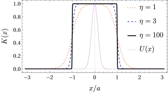
Figure 2: $K(x)$ defined in Eq. 21 for various values of $\eta$ compared with $U(x)$ defined in Eq. 22 with $\Gamma=1$ and $b=0.2$ . As $\eta\rightarrow\infty$, $K(x)$ takes the form shown in Eq. 23.

Let us now consider the classical trajectories of dipole-conserving systems in one dimension with identical charge and mass (both of which we set to unity without any loss of generality). The dipole moment $D=\sum_{a}x_{a}$ is proportional to the center-of-mass (COM). This is perfectly dual to the conservation of the center of momentum imposed by translation invariance:

Translation: $$x_{a}\mapsto x_{a}+\xi,~{}P=\sum_{a}p_{a}\text{ conserved.}$$

Dipole: $$p_{a}\mapsto p_{a}+\phi,~{}D=\sum_{a}x_{a}\text{ conserved.}$$

The Hamiltonian of Eq. 17 now takes on the following simple form:

$$H=\sum_{a<b=1}^{N}\left[\frac{1}{2}\left(p_{a}-p_{b}\right)^{2}K(x_{a}-x_{b})+U(x_{a}-x_{b})\right].$$ (20)

For concreteness, we will use the following forms of $K(x)$ and $U(x)$

$$K(x) =\frac{1}{2}\left[\tanh\left(\eta\left(x+a\right)\right)-\tanh\left(\eta\left(x-a\right)\right)\right],$$ (21)

$$U(x) =\Gamma\exp\left(-\frac{x^{2}}{b^{2}}\right).$$ (22)

although we expect all our results to hold for any other physically sensible choices. $\Gamma$ denotes the interaction strength and can be attractive or repulsive. $\Gamma=0$ represents the closest equivalent to free particles. $K(x)$ is a positive definite function which vanishes at $|x|\rightarrow\infty$ and has the limiting form

$$\lim\limits_{\eta\rightarrow\infty}K(x)\equiv B(x)=\Theta(x+a)-\Theta(x-a),$$ (23)

as shown in Fig. 2, where $\Theta(x)$ is the Heaviside Theta function. We now have two length-scales in the Hamiltonian Eq. 20– $a$ represents the separation scale below which the kinetic term is operative and two fractons can ‘lend inertia’ to each other and $b$ represents the interaction range between particles. We will only consider the case of $a>b$.

III.1.2 Far-separated particles and general features

Figure 3: Sample particle configuration in d=1 where each particle is far separated from the others and is immobile.

Let us study a configuration that immediately exposes general features of dynamics generated by the Hamiltonian shown in Eq. 20 by switching off the interactions ($U(x)=0$) and set $\eta\rightarrow\infty$ when $K(x)$ takes the form shown in Eq. 23. For initial conditions when particles are well-separated $(x_{a}(0)-x_{b}(0))>>a$ as shown in Fig. 3, the Hamiltonian Eq. 20 vanishes and the particles are all completely frozen. Thus, we have a large manifold of zero-energy configurations where each particle is isolated within an independent Machian cluster and is therefore immobile. This is consistent with the expectation that locally isolated fractons are immobile [1, 2]. A distinct feature however is that even though the particles have vanishing velocities, their momenta $\{p_{a}(0)\}$ are completely undetermined and can be arbitrarily fixed. The disassociation between energy, velocities and momenta has two sources of origin. First is the exact microscopic symmetry as discussed in as discussed in Section II.3 – dipole conservation results in a many-to-one relationship between momenta and velocity. When initial particle separation is large however, not only is the total dipole moment $D=\sum_{a}x_{a}$ conserved, the coordinate of each particle $x_{a}$ is itself conserved and the conserved total dipole moment fragments to $N$ conserved positions, $x_{a}$. This brings us to the second origin for the velocity-momentum-energy mismatch– emergent symmetries. The conserved quantities $x_{a}$ now generate a larger symmetry wherein each momentum can be arbitrarily shifted $p_{a}\mapsto p_{a}+\phi_{a}$. This holds as we move away from the $U(x)\rightarrow 0,\eta\rightarrow\infty$ limit. When particles are well-separated compared to the length-scales set by $K(x)$ and $U(x)$ and momentum differences are such that

$$\left(p_{a}-p_{b}\right)^{2}K(x_{a}-x_{b})\rightarrow 0,$$

the Hamiltonian Eq. 20 vanishes and the discussion above holds.

For particles starting with close initial separation, the situation is more complex and will be discussed in detail for the remainder of this section. By numerically solving Hamilton’s equations of motion for the Hamiltonian in Eq. 20, we will see that velocity-momentum mismatch as well as emergent conserved quantities will generically appear accompanying qualitatively new kinds of trajectories. All computations were performed using Wolfram Mathematica [18].

Before we proceed, let us point out a useful canonical transformation $\{x_{j},p_{j}\}\mapsto\{q_{\alpha},\pi_{\alpha}\}$ that we will occasionally employ

$$q_{\alpha=1,\ldots,N-1} =\frac{\sum_{j=1}^{\alpha}x_{j}-\alpha x_{\alpha+1}}{\sqrt{\alpha\left(\alpha+1\right)}},~{}q_{N}=\frac{\sum_{j=1}^{N}x_{j}}{\sqrt{N}},$$

$$\pi_{\alpha=1,\ldots,N-1} =\frac{\sum_{j=1}^{\alpha}p_{j}-\alpha p_{\alpha+1}}{\sqrt{\alpha\left(\alpha+1\right)}},~{}\pi_{N}=\frac{\sum_{j=1}^{N}p_{j}}{\sqrt{N}}.$$ (24)

Notice that $q_{N}=D/\sqrt{N}$ and $\pi_{N}=P/\sqrt{N}$ are the conserved quantities. These drop out when we express the Hamiltonian Eq. 20 using Eq. 24 making the translation and dipole symmetries manifest,

$$H(x_{1},\ldots x_{N};p_{1},\ldots p_{N})=H(q_{1},\ldots q_{N-1};\pi_{1},\ldots\pi_{N-1})\\ \implies\{H,q_{N}\}=\{H,\pi_{N}\}=0.$$ (25)

This helps us reduce the effective phase space of $N$ particles to that of $N-1$ particles. We will refer to $\{q_{\alpha},\pi_{\alpha}\}$ as reduced phase space coordinates.

III.2 Two fractons on a line

Figure 4: Two closely separated particles in the same Machian cluster exhibit two classes of trajectories. For negative energies which are possible when interactions are attractive ($U<0$), the particles exhibit regular trajectories where they oscillate out of phase preserving the centre of mass. For positive energies, they exhibit novel fractonic trajectories where they eventually separate and freeze to form two adjacent clusters.

III.2.1 Trajectories

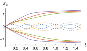
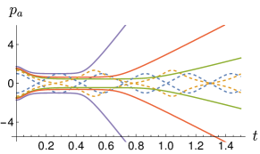
Figure 5: Two particle trajectories generated by Eq. 26 for attractive interactions ($a=1,b=0.2,\eta=10,\Gamma=-1$ ). Negative energies (dotted, $E=-0.5,-0.1$) lead to oscillatory trajectories with bounded position and momentum coordinates. Positive energies (solid, $E=0.1,0.2,0.5$) lead to ‘fractonic’ trajectories where the position coordinates freeze out while the momenta grow indefinitely.

Let us consider two particles within a single Machian cluster i.e. in close initial separation such that $K(x_{1}(0)-x_{2}(0))\neq 0$ . To analyse the ensuing dynamics, we begin by expressing its Hamiltonian in reduced coordinates shown in Eq. 24 to eliminate the conserved dipole moment and total momentum, $q_{2},\pi_{2}$ thereby reducing the phase space to that of a single degree of freedom:

$$H=\pi_{1}^{2}K(\sqrt{2}q_{1})+U(\sqrt{2}q_{1}).$$ (26)

We still have one remaining conserved quantity– Energy (E) using which Hamilton’s equations of motion can be formally solved by quadrature as follows

$$t=\int_{q(0)}^{q(t)}\frac{dy}{2\sqrt{K(\sqrt{2}y)\left(E-U(\sqrt{2}y)\right)}},$$

$$\pi(t)=\sqrt{\frac{E-U(\sqrt{2}q(t))}{K(\sqrt{2}q(t))}}.$$ (27)

There are two possible classes of trajectories depending on the energy of the system and the nature of interactions. For negative energy configurations, available with attractive interactions ($\Gamma<E<0$), we get familiar oscillating solutions, shown in Fig. 5 with dotted lines. The two particles stay within a single Machian cluster and oscillate precisely out of phase to conserve centre of mass. Both position and momentum coordinates are bounded. For small oscillations, the frequency $\omega_{0}$ can be determined by setting $K\approx 1$ and Taylor expanding $U$ in Eq. 26 to get

$$H\approx\pi_{1}^{2}+\frac{2|\Gamma|}{b^{2}}x^{2}\implies\omega_{0}\approx\sqrt{\frac{8|\Gamma|}{b^{2}}}.$$ (28)

For positive energy configurations, we find a novel class of trajectories. Irrespective of the nature of interactions (attractive $U<0$, repulsive $U>0$ or no interactions $U=0$), we find that all trajectories with $E>0$ follow a similar pattern– particles starting within a single Machian cluster eventually drift apart in opposite directions, conserving the centre-of-mass and eventually become immobile as they end up isolated in two adjacent clusters. One curious aspect of these trajectories is that as the particles separate we have $K(x_{1}-x_{2})\rightarrow 0$ and $U(x_{1}-x_{2})\rightarrow 0$ in Eq. 26. The system conserves energy by $|p_{1}-p_{2}|\rightarrow\infty$ at late times appropriately. We call these trajectories ‘fractonic’ to distinguish from ordinary trajectories present in dipole non-conserving systems where diverging momenta are not typically found. Sample fractonic trajectories are shown Fig. 5 using solid lines.

III.2.2 Dissipative dynamics and attractors

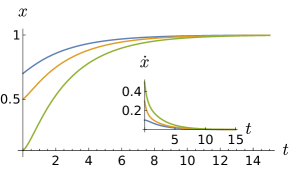
Figure 6: $\{x,\dot{x}\}$ trajectories (top) for the over-damped oscillator governed by Eq. 29 with $m=k=a=1,\mu=3$ compared with the fractonic trajectories (bottom) corresponding to positive energies $E=0.4,0.5,1.0$ for the two-particle system generated by the Hamiltonian in Eq. 26 with $a=1,b=0.2,\eta=20$ and $\Gamma=-1$ in reduced (configuration) space coordinates $\{q_{1},\dot{q_{1}}\}$ .

Consider a one-dimensional classical oscillator living a viscous environment governed by the following equation of motion

$$m\ddot{x}=-\mu\dot{x}-k(x-a).$$ (29)

The trajectories of Eq. 29 are shown in the top row of Fig. 6 in the over-damped limit, $\mu>2\sqrt{km}$ for various initial configurations. We see that the particle slows down with time and eventually becomes immobile. This dynamics is qualitatively the same as that of two-particles discussed in Section III.2 whose trajectories in the reduced coordinates are shown in the bottom row of Fig. 6 for comparison. The crucial difference is that in the case of the dissipative particle, momentum is related to velocity in the usual way– $p=m\dot{x}$ whereas in the case of fractons, it is not.

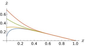
Figure 7: Configuration space portrait for the overdamped oscillator (top) with $m=k=a=1,\mu=3$ compared with the dipole conserving two-particle system in reduced coordinates (bottom) with $a=1,b=0.2,\eta=20$ and $\Gamma=-1$. Both exhibit attractive fixed-points where multiple trajectories terminate.

Dissipative dynamics is accompanied by the presence of attractors in configuration (position, velocity) space– as $t\rightarrow\infty$, all trajectories of the dissipative particle shown in Fig. 6 approach the same point $(x,\dot{x})=(a,0)$ as shown in Fig. 7. For dipole conserving systems on the other hand, as shown in Fig. 7, the two classes of trajectories described above correspond to two types of fixed points. The first, at the origin $(q_{1},\dot{q}_{1})=\left(0,0\right)$ is a center [19] which is surrounded by negative energy oscillatory trajectories. The second, remarkably, are attractors at $(q_{1},\dot{q}_{1})\approx\left(\pm\frac{a}{\sqrt{2}},0\right)$ where fractonic trajectories terminate. These are surprising because Liouville’s theorem forbids such attractors in (position-momentum) phase space for Hamiltonian systems. For ordinary (dipole non-conserving) Hamiltonian systems with $p=m\dot{x}$, this implies that there are also no attractors in (position-velocity) configuration space. For fractonic trajectories in dipole conserving systems however, we see that the absence of attractors in phase space does not translate into the absence of attractors in configuration space!

III.3 Three fractons on a line

Figure 8: Three closely separated particles in the same Machian cluster exhibit three classes of trajectories. For negative energies which are possible when interactions are attractive ($U<0$), the particles exhibit regular oscillations or chaos preserving the centre of mass. For positive energies, they exhibit fractonic trajectories where two particles settle to an oscillatory state in one cluster while the third freezes out in another.

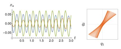
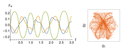
Figure 9: Non-fractonic regular (top, $E=-2.5$) and chaotic (bottom, $E=-1$) trajectories of three particle position ($x_{a}$) coordinates along with corresponding two-dimensional phase portraits in reduced coordinates ($q_{1}-q_{2}$) generated by the Hamiltonian in Eq. 30 with $a=1,b=0.2,\eta=10$ and $\Gamma=-1$.

We now consider three particles. The Hamiltonian Eq. 20 for $N=3$ in reduced coordinates Eq. 24 contains two effective degrees of freedom operating on a four dimensional phase-space $(q_{1},\pi_{1},q_{2},\pi_{2})$.

$$H=\pi_{1}^{2}K(\sqrt{2}q_{1})+\frac{\left(\sqrt{3}\pi_{2}+\pi_{1}\right)^{2}}{4}K\left(\frac{\sqrt{3}q_{2}+q_{1}}{\sqrt{2}}\right)\\ +\frac{\left(\sqrt{3}\pi_{2}-\pi_{1}\right)^{2}}{4}K\left(\frac{\sqrt{3}q_{2}-q_{1}}{\sqrt{2}}\right)+U(\sqrt{2}q_{1})\\ +U\left(\frac{\sqrt{3}q_{2}+q_{1}}{\sqrt{2}}\right)+U\left(\frac{\sqrt{3}q_{2}-q_{1}}{\sqrt{2}}\right).$$ (30)

III.3.1 Trajectories

Just like in the case of two particles we again see non-fractonic trajectories for certain negative energies with attractive interactions ($\Gamma<0$). Unlike the two particle case however, these can now be regular or chaotic as seen in Fig. 9. The appearance of non-fractonic chaotic and regular trajectories in a system with two degrees of freedom is familiar and qualitatively the same as the Hénon Helies model  [20]. However, the latter has free trajectories where the particles travel with constant momenta whereas the former has fractonic trajectories instead.

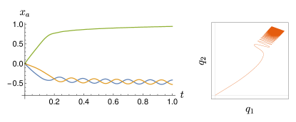
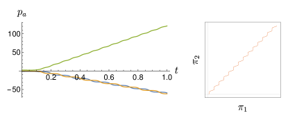
Figure 10: Fractonic trajectories ($E=10$) of three particle position ($x_{a}$) and momentum ($p_{a}$) coordinates along with corresponding two-dimensional phase portraits in reduced coordinates ($q_{1},q_{2}$) generated by the Hamiltonian in Eq. 30 with $a=1,b=0.2,\eta=10$ and $\Gamma=-1$.

Fractonic trajectories are found for both positive and negative energy configurations and therefore for attractive ($\Gamma<0$), repulsive ($\Gamma>0$) or indeed no interactions ($\Gamma=0$). These are qualitatively different from the fractonic trajectories of two-particles. A direct extrapolation of the two-particle picture suggests that at late times, we expect the particles starting within each other’s presence in a single cluster to separate out until they are isolated within their own separate Machian clusters and become immobile. In fact, this scenario only occurs for fine-tuned initial conditions as will be proven within an exactly solvable limit in Section V. As shown in Fig. 10, we see that generically, fracton trajectories corresponds to the system breaking up with one of the particles separating out from the other two and eventually becoming immobile. On the other hand, the remaining two particles form a single cluster and settle down to an indefinite oscillatory state about their common centre of mass. Interestingly, these oscillations result from the particles bouncing off the edge of the Machian cluster of the first particle.

In summary, generically, when three particles start off within a single cluster, fractonic trajectories lead to the formation of atleast two separate clusters. For certain fine-tuned conditions as will be discussed in Section V, fractonic trajectories lead to three isolated clusters.

III.3.2 Limit cycles

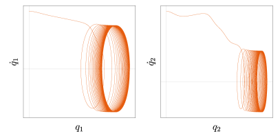
Figure 11: Projections of the reduced coordinate configuration phase portrait of the fractonic trajectory shown in Fig. 10 exhibits a limit-cycle behaviour.

We saw in Section III.2 that fractonic trajectories for two particles ended up in an attractor in the position-velocity configuration space. For three particles, generic fracton trajectories asymptotically end up in a limit-cycle as shown in Fig. 11 in configuration space. Just like attractors, Liouville’s theorem forbids the presence of limit cycles in phase space which, for non-dipole-conserving systems where velocities are proportional to momenta, also implies the absence of limit cycles in configuration space. For fractons, this is no longer true and while mathematical limit cycles are not to be found in phase space, consistent with Liouville’s theorem, physical limit cycles do appear in configuration space!

III.4 Four and more fractons on a line

Figure 12: Four closely separated particles in the same Machian cluster exhibit three classes of fractonic trajectories. Asymptotically, the system can separate into two clusters with two particles each where each pair exhibits oscillatory trajectories (top) or one frozen particle in one cluster and three in the other, exhibiting either regular oscillations or chaos (bottom).

We now turn to the final case of four particles. The Hamiltonian written in reduced coordinates is now a function of six phase space coordinates corresponding to three degrees of freedom. We will not write the explicit form here. With attractive interactions, we again obtain non-fractonic bounded oscillatory and chaotic trajectories qualitatively similar to the three-particle case shown in Fig. 9. We will therefore switch off the interactions ($U(x)=0$) for the rest of this section and focus only on fractonic trajectories.

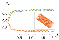
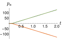
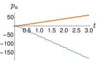
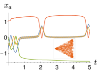
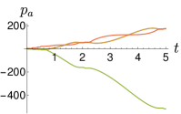
Figure 13: Fractonic regular trajectories exhibiting three-particle oscillations (top), two particle oscillations (middle) and chaos (bottom) generated by the four-particle Hamiltonian without interactions Eq. 20 with $E=10$ and $a=1,\eta=10$ and $\Gamma=0$. The insets show reduced coordinate $q_{1},q_{2}$ projections of phase portraits where the regular and chaotic nature of trajectories are clearer.

As shown in Fig. 13, we find that four particles starting within a single Machian cluster eventually separate into two. The nature of asymptotic dynamics in each of the two asymptotic clusters now depends sensitively on initial conditions. Figure 13, shows samples of the various trajectories possible for the same fixed energy and Hamiltonian parameters but different initial conditions. We see two classes of regular fractonic trajectories (top two rows) where the four particles split into subsystems with two-two or three-one particles and the multi-particle subsystems settle down into indefinite oscillations at late times. These are qualitatively similar to the fractonic trajectories for three particles shown in Fig. 10. The bottom figure in Fig. 13 represents a new class of fracton trajectories where the four particles split into three-one particle subsystems and the three particles exhibit chaos. Like the regular fracton trajectories, the chaotic fracton trajectory has momenta that grow indefinitely with time.

We can conjecture that the trajectories studied above for four or fewer particles qualitatively exhausts all possibilities for a finite number of fractons – particles within a single Machian cluster exhibit either (i) non-fractonic regular or chaotic dynamics in the same cluster or (ii) fractonic regular or chaotic dynamics where the system asymptotically splits into multiple Machian clusters. We have checked this numerically for systems with various number of particles starting in close proximity and several randomly generated initial conditions.

IV Oppositely charged fractons on a line

We now relax the conditions of Section III and consider the case where not all particles carry the same charge. We will only consider the case with no interactions i.e. $U(x)=0$. The Hamiltonian in Eq. 20 is modified to

$$H=\frac{1}{2}\sum_{a<b=1}^{N}\left(\frac{p_{a}}{q_{a}}-\frac{p_{b}}{q_{b}}\right)^{2}K(x_{a}-x_{b}).$$ (31)

As discussed in Section II, the conserved dipole moment and the symmetry transformation induced by it are

$$D=\sum_{a}q_{a}x_{a},~{}\dot{D}=0\implies p_{a}\mapsto p_{a}+q_{a}\phi.$$ (32)

For concreteness, let us consider the charge assignment $q_{a}=(-1)^{a}$ so that we have two species of particles with charges $\pm 1$ and the form of $K(x)$ as shown in Eq. 21. The whole system is net charge neutral for even number of particles. The main new possibility that opens up is that of particles pairing up into charge neutral dipoles which can in principle behave like ordinary non-fractonic particles. The simplest case to consider is two particles.

IV.1 Two oppositely charged fractons

The two-particle version of the Hamiltonian in Eq. 31

$$H=\frac{1}{2}\left(p_{1}+p_{2}\right)^{2}K(x_{1}-x_{2}).$$ (33)

The Hamiltonian is entirely a function of the conserved quantities– the total dipole moment $D=x_{1}-x_{2}$ and momentum $P=p_{1}+p_{2}$

$$H=\frac{P^{2}}{2}K(D).$$ (34)

The equations of motion can be trivially solved to get

$$x_{a}(t) =x_{a}(0)+PK(D)t,$$

$$p_{a}(t) =p_{a}(0)-(-1)^{a}\frac{P^{2}}{2}K^{\prime}(D)t.$$ (35)

The two particles moves together as a dipole unit with a fixed separation and with a constant velocity, $v_{\text{eff}}=PK(D)$. In other words, the dipole moves as a free particle with an effective dipole moment- dependent mass $m_{\text{eff}}=K(D)^{-1}$. As we separate the two particles, we increase the dipole moment and therefore the mass. Particles with a large separation therefore once again become completely immobile. This qualitative picture for the motion of opposite-charged pair of fractons was also seen in [8]. Finally, let us observe that while the momentum of the centre of mass is constant, individual momenta evolve with time as shown in Eq. 35 and increase indefinitely with time.

IV.2 Many oppositely charged fractons

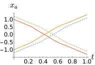
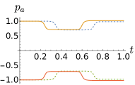
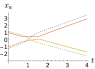
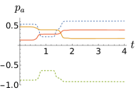
Figure 14: Trajectories generated by the four particle Hamiltonian in Eq. 31 with $a=1$ and $\eta=10$ showing asymptotic free dipole motion. Positive (negative) charge motion is described with solid (broken) lines. When the dipoles meet, they may not (top) or may (bottom) exchange partners.

With a larger number of particles, new possibilities emerge. One straightforward generalization of the two-particle case is that dipoles move as free particles in isolation from other particles. However, when two dipoles meet, they can interact due to the locality term $K(x)$. They can either (i) pass through each other when they meet as shown in the top column of Fig. 14 or (ii) exchange partners by swapping particles of like charge between dipole units as shown in the bottom column of Fig. 14. However, more complex trajectories are also possible wherein the system clusters in various ways and like particles exhibit fractonic trajectories described in Section III. Samples of these complex trajectories are shown in Fig. 15.

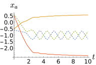
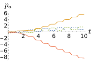
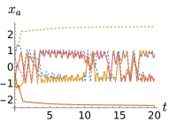
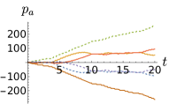
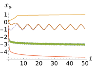
Figure 15: Fractonic trajectories generated by the four particle (top) and six particle (middle, bottom) Hamiltonians of Eq. 31 with $a=1$ and $\eta=10$. Positive (negative) charge motion is described with solid (broken) lines. We see the formation of multiple clusters each of which exhibits fractonic regular and chaotic motion with unbounded momentum growth.

V Exact solutions

In this section, we consider a limit wherein fracton trajectories of like particles can be obtained exactly. This will confirm the numerical trajectories shown in Section III. For this, we consider the Hamiltonian Eq. 20, switch off interactions $U(x)=0$ and set $\eta\rightarrow\infty$ to get

$$H=\frac{1}{2}\sum_{a<b}B(x_{a}-x_{b})\left(p_{a}-p_{b}\right)^{2}$$ (36)

where, $B(x)$ is the as defined in Eq. 23. For this form, we can obtain exact, regular fractonic trajectories for upto three particles. Since a solution by quadrature shown in Eq. 27 exists for the two-particle Hamiltonian Eq. 26, the non-trivial case is three-particles. We will discuss the solution for two-particles as a warm up and then proceed to three-particles.

V.1 Warm-up: Two particles

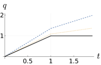
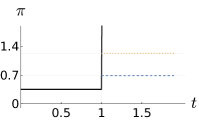
Figure 16: Plot of exact trajectories shown in Eq. 44 for $\delta=0.6$ (dashed line), $0.3$ (dotted line) and $0$ (solid line). Initial conditions chosen as $q(0)=0,~{}\pi(0)=(2\sqrt{2})^{-1}$ and we set $a=\sqrt{2}$. The Grid lines mark $t^{*}=1$ on $t$ axis, $\sqrt{2}q=a$ on the $q$ axis and $\pi_{>}$ for each delta determined from Eq. 43 on the $\pi$ axis.

The Hamiltonian in Eq. 36 for two particles written in terms of the reduced coordinates shown in Eq. 24 is

$$H=\pi_{1}^{2}B(\sqrt{2}q_{1}).$$ (37)

We will henceforth drop the redundant subscript $\{q_{1},\pi_{1}\}\equiv\{q,\pi\}$ to reduce clutter. We will only concern ourselves with initial conditions such that Eq. 37 does not vanish i.e. $|q(0)|<a/\sqrt{2}$ and $\pi(0)\neq 0$. We want to solve Hamilton’s equations of motion,

$$\dot{q}=2\pi B(\sqrt{2}q),~{}\dot{\pi}=-\sqrt{2}\pi^{2}B^{\prime}(\sqrt{2}q).$$ (38)

To do this, we first regulate $B(x)$ so it does not vanish for any value of $x$

$$B(x)\rightarrow B(x)+\delta^{2}$$ (39)

and eventually take $\delta\rightarrow 0$. Notice that when $|q|\neq a/\sqrt{2}$, the equations in Eq. 38 reduce to those of free particles. Naturally, our strategy will be to solve Eq. 38 piecewise and then stitch up the solutions. For $|q_{1}(0)|<a/\sqrt{2}$, we have $B^{\prime}(\sqrt{2}q)=0$ and $B(\sqrt{2}q)=1+\delta^{2}$ and Eq. 38 can be integrated to get

$$\pi(t)=\pi(0),~{}q(t)=q(0)+2\pi(0)(1+\delta^{2})t.$$ (40)

The solution in Eq. 40 holds for $t<t^{*}$ where $t^{*}$ is defined by the condition

$$|q(t^{*})|=a/\sqrt{2}.$$ (41)

For $t>t^{*}$, we have $|q|>a/\sqrt{2}$ and therefore $B^{\prime}(\sqrt{2}q)=0$ and $B(\sqrt{2}q)=\delta^{2}$. Equation 38 can again be solved to get

$$\pi(t)=\pi_{>},~{}q(t)=q(t^{*})+2\pi_{>}\delta^{2}t,$$ (42)

where, $q(t^{*})=\text{sgn}(\pi(0))a/\sqrt{2}$. $\pi_{>}$ can be determined using energy conservation.

$$E(q(t<t^{*}),\pi(t<t^{*}))=E(q(t>t^{*}),\pi(t>t^{*}))\\ \implies\pi_{>}=\pi(0)\frac{\sqrt{1+\delta^{2}}}{\delta}.$$ (43)

Substituting into Eq. 42 we get the full piecewise defined solution,

$$q(t) =\begin{cases}q(0)+2\pi(0)t(1+\delta^{2})&t<t^{*}\\ q(t^{*})+2\pi(0)(t-t^{*})\delta\sqrt{1+\delta^{2}}&t>t^{*}\end{cases}$$

$$\pi(t) =\begin{cases}\pi(0)&t<t^{*}\\ \pi(0)\frac{\sqrt{1+\delta^{2}}}{\delta}&t>t^{*}\end{cases}.$$ (44)

We can now take $\delta\rightarrow 0$ and remove the regulator to finally get

$$q(t) =\begin{cases}q(0)+2\pi(0)t&t<t^{*}\\ q(t^{*})&t>t^{*}.\end{cases}$$

$$\pi(t) =\begin{cases}\pi(0)~{}~{}~{}~{}t<t^{*}\\ \infty~{}~{}~{}~{}~{}~{}~{}t>t^{*}\end{cases}$$ (45)

This qualitatively confirms the nature of two-particle fracton trajectories shown in Section III.2.

V.2 Symmetries and distinct sectors for three particles

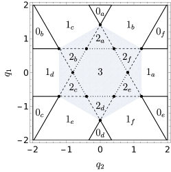
Figure 17: Distinct regimes of the three-particle Hamiltonian in Eq. 47. The labels $M_{a},M_{b}$ etc. indicate the number of particle pairs $M$ that are proximate such that Eq. 48 holds. The shaded region surrounding the origin represents the initial conditions that can lead to an oscillating steady state.

We now move on to the three-particle case which is our main interest in this section. The Hamiltonian Eq. 36 we want to consider is

$$H=H_{12}+H_{13}+H_{23}$$ (46)

where, $H_{ab}\equiv\frac{1}{2}(p_{a}-p_{b})^{2}B(|x_{a}-x_{b}|)$. In reduced coordinates, this corresponds to the the following Hamiltonian acting on the four-dimensional phase space of two degrees of freedom

$$H=\pi_{1}^{2}B(\sqrt{2}q_{1})+\frac{\left(\sqrt{3}\pi_{2}+\pi_{1}\right)^{2}}{4}B\left(\frac{\sqrt{3}q_{2}+q_{1}}{\sqrt{2}}\right)\\ +\frac{\left(\sqrt{3}\pi_{2}-\pi_{1}\right)^{2}}{4}B\left(\frac{\sqrt{3}q_{2}-q_{1}}{\sqrt{2}}\right).$$ (47)

We will use the form in Eq. 47 for the rest of this section. Let us begin by dividing the two-dimensional position-space $\{q_{1},q_{2}\}$ into different sectors depending on how many pairs of particles are proximate to each other i.e. the number of pairs $(a,b)$ such that

$$|x_{a}-x_{b}|<a\implies B(|x_{a}-x_{b}|)=1.$$ (48)

This is summarized in Fig. 17 where the labels $0,1,2,3$ represent the number of pairs satisfy Eq. 48. The Hamiltonian in Eq. 47 has the symmetries of a regular hexagon manifest in Fig. 17, generated by reflections and six-fold rotations. The action of these symmetries on phase-space coordinates are

$$\{\vec{q}\mapsto R\vec{q},~{}\vec{\pi}\mapsto R\vec{\pi}\},~{}R=\begin{pmatrix}~{}~{}\cos\omega&\sin\omega\\ -\sin\omega&\cos\omega\end{pmatrix}\text{ and}$$

$$\{\vec{q}\mapsto X\vec{q},~{}\vec{\pi}\mapsto X\vec{\pi}\},~{}X=\begin{pmatrix}1&0\\ 0&-1\end{pmatrix},$$ (49)

where $\vec{q}\equiv\begin{pmatrix}q_{1},q_{2}\end{pmatrix}^{T},~{}\vec{\pi}\equiv\begin{pmatrix}\pi_{1},\pi_{2}\end{pmatrix}^{T}$.

Together, $R$ and $X$ form an irreducible representation of the dihedral group $D_{12}$ [21]. The invariance of the Hamiltonian Eq. 47 under Eq. 49 is useful because it maps the various sectors $\{M_{a}\ldots M_{f}\}$ shown in Fig. 17 into each other. Consequently, trajectories with one set of initial conditions can be used to generate trajectories with other initial conditions by symmetry transformations which allows us to restrict our attention to only a representative set of cases.

The Hamilton’s equations of motion (eom) for Eq. 47, which we seek to solve are

$$\dot{q}_{1} =\frac{\partial H}{\partial\pi_{1}}=\frac{\left(\sqrt{3}\pi_{2}+\pi_{1}\right)}{2}B\left(\frac{\sqrt{3}q_{2}+q_{1}}{\sqrt{2}}\right)$$

$$-\frac{\left(\sqrt{3}\pi_{2}-\pi_{1}\right)}{2}B\left(\frac{\sqrt{3}q_{2}-q_{1}}{\sqrt{2}}\right)+2\pi_{1}B(\sqrt{2}q_{1}),$$

$$\dot{q}_{2} =\frac{\partial H}{\partial\pi_{2}}=\frac{\sqrt{3}\left(\sqrt{3}\pi_{2}+\pi_{1}\right)}{2}B\left(\frac{\sqrt{3}q_{2}+q_{1}}{\sqrt{2}}\right)$$

$$~{}~{}~{}~{}~{}~{}~{}~{}~{}~{}+\frac{\sqrt{3}\left(\sqrt{3}\pi_{2}-\pi_{1}\right)}{2}B\left(\frac{\sqrt{3}q_{2}-q_{1}}{\sqrt{2}}\right),$$

$$\dot{\pi}_{1} =-\frac{\partial H}{\partial q_{1}}=-\frac{\left(\sqrt{3}\pi_{2}+\pi_{1}\right)^{2}}{4\sqrt{2}}B^{\prime}\left(\frac{\sqrt{3}q_{2}+q_{1}}{\sqrt{2}}\right)$$

$$-\sqrt{2}\pi_{1}^{2}B^{\prime}(\sqrt{2}q_{1})+\frac{\left(\sqrt{3}\pi_{2}-\pi_{1}\right)^{2}}{4\sqrt{2}}B^{\prime}\left(\frac{\sqrt{3}q_{2}-q_{1}}{\sqrt{2}}\right),$$

$$\dot{\pi}_{2} =-\frac{\partial H}{\partial q_{2}}=-\frac{\sqrt{3}\left(\sqrt{3}\pi_{2}+\pi_{1}\right)^{2}}{4\sqrt{2}}B^{\prime}\left(\frac{\sqrt{3}q_{2}+q_{1}}{\sqrt{2}}\right)$$

$$~{}~{}~{}~{}~{}~{}~{}~{}~{}~{}~{}-\frac{\sqrt{3}\left(\sqrt{3}\pi_{2}-\pi_{1}\right)^{2}}{4\sqrt{2}}B^{\prime}\left(\frac{\sqrt{3}q_{2}-q_{1}}{\sqrt{2}}\right).$$ (50)

We follow the general strategy used for the two particle case. Away from the boundaries shown in Fig. 17, we can set $B(\ldots)=0$ or $1$ (depending on the sector) and $B^{\prime}(\ldots)=0$ in Eq. 50 when we have a free trajectory for $q_{1}$ and $q_{2}$ while $\pi_{1}$ and $\pi_{2}$ are constant. These are stitched together at the boundaries shown in Fig. 17 where the momentum jumps discontinuously. We first write down representative piecewise solutions and then evaluate the jump conditions.

V.3 Piecewise solutions

Let us write down solutions for trajectories within the various sectors listed in Fig. 17 away from the boundaries. Irrespective of the sector we are considering, $B^{\prime}(\ldots)$ vanishes and momenta remain constant in time

$$\dot{\pi}_{\alpha}=0\implies\pi_{\alpha}(t)=\pi_{\alpha}(0).$$ (51)

The evolution of position coordinates $q_{\alpha}$ takes on the form

$$q_{\alpha}(t)=q_{\alpha}(0)+\dot{q}_{\alpha}(0)t.$$ (52)

The velocities $\dot{q}_{\alpha}(0)$ are determined from the constant momenta $\pi_{\alpha}(0)$ in different ways depending on the sector. Let us begin with $\{0_{a}\ldots 0_{f}\}$ where all $B(\ldots)$ vanish in Eq. 50 and we have

$$\boxed{0_{a-f}:~{}\dot{q}_{\alpha}=0\implies q_{\alpha}(t)=q_{\alpha}(0).}$$ (53)

We reproduced the result discussed earlier in Fig. 3 that for particles that are well-separated, the Hamiltonian vanishes, each phase-space coordinate is a constant of motion and dynamics is completely frozen.

Let us now consider the sectors $\{1_{a},\ldots,1_{f}\}$. Due to the symmetry discussed above, these sectors map into each other and it suffices to consider one representative. We choose $1_{a}$ with no loss of generality. Here, $B(\sqrt{2}q_{1})=1$ while $B\left(\frac{\sqrt{3}q_{2}\pm q_{1}}{\sqrt{2}}\right)=0$. This gives us

$$\boxed{1_{a}:\begin{cases}\dot{q}_{1}=2\pi_{1}&\implies q_{1}(t)=q_{1}(0)+2\pi_{1}(0)t,\\ \dot{q}_{2}=0~{}~{}~{}&\implies q_{2}(t)=q_{2}(0).\end{cases}}$$ (54)

Observe that the trajectories in Eq. 54 do not depend at all on the value of $\pi_{1}(0)$ and there is no motion in the direction where the sector $1_{a}$ is extended. By rotation, this feature is true for the other sectors $1_{b}\ldots 1_{f}$– motion is entirely along the direction perpendicular to the strip on which the sector is defined and frozen in the parallel direction.

Let us now consider the sectors $\{2_{a},\ldots,2_{f}\}$. We choose $2_{a}$ with no loss of generality. Here, $B\left(\frac{\sqrt{3}q_{2}\pm q_{1}}{\sqrt{2}}\right)=1$ and $B(\sqrt{2}q_{1})=0$ and we get

$$\boxed{2_{a}:\begin{cases}\dot{q}_{1}=\pi_{1}&\implies q_{1}(t)=q_{1}(0)+\pi_{1}(0)t,\\ \dot{q}_{2}=3\pi_{2}&\implies q_{2}(t)=q_{2}(0)+3\pi_{2}(0)t.\end{cases}}$$ (55)

Finally, consider the sector $3$ when all $B(\ldots)=1$ and we get

$$\boxed{3:\begin{cases}\dot{q}_{1}=3\pi_{1}&\implies q_{1}(t)=q_{1}(0)+3\pi_{1}(0)t,\\ \dot{q}_{2}=3\pi_{2}&\implies q_{2}(t)=q_{2}(0)+3\pi_{2}(0)t.\end{cases}}$$ (56)

V.4 Jump conditions

The piecewise solutions shown in Eqs. 53, 54, 55 and 56 apply away from the boundaries shown in Fig. 17. We now discuss what happens at the boundaries. As shown in Fig. 17, there are two types of boundaries – lines where two sectors meet and points where more than two sectors meet. At these boundaries, we expect the momenta $\pi_{1}$ and $\pi_{2}$ to discontinuously jump. The best way we have found to quantify this jump is to use conservation of energy along with combinations of the momentum eom in Eq. 50 that can be easily handled in an integrated form. We will describe this strategy in detail below for a representative of each type of boundary.

$3-2_{a}$ boundary

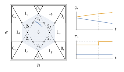
Figure 18: Numerical plots of a trajectory passing from $3$ to $2_{a}$ (solid line) obtained for large $\eta$ compared with jump location and magnitudes predicted from the exact solution shown in Eq. 62 (broken lines).

Let us begin with the boundary between sectors $3$ and $2_{a}$ corresponding to the segment

$$q_{1}=\frac{a}{\sqrt{2}},~{}-\frac{a}{\sqrt{6}}<q_{2}<\frac{a}{\sqrt{6}},$$ (57)

as shown in Fig. 17 and consider the possibility of the trajectory passing this line starting from either side. We want to find how the momenta in the two sectors, $\pi_{\alpha}^{[3]}$ and $\pi_{\alpha}^{[2_{a}]}$ are related to each other. The relationship between momenta and energy in these sectors are

$$E{[3]} =\frac{3}{2}\left(\left(\pi_{1}^{[3]}\right)^{2}+\left(\pi_{2}^{[3]}\right)^{2}\right),$$ (58)

$$E{[2_{a}]} =\frac{1}{2}\left(\left(\pi_{1}^{[2_{a}]}\right)^{2}+3\left(\pi_{2}^{[2_{a}]}\right)^{2}\right).$$ (59)

Conservation of energy, $E{[2_{a}]}=E[3]$ giving us one relationship between $\pi_{\alpha}^{[3]}$ and $\pi_{\alpha}^{[2_{a}]}$. A second one can be obtained by considering the equations of motion shown in Eq. 50. Note that as the trajectory passes through the line separating sectors $3$ and $2_{a}$, the condition $B^{\prime}\left(\frac{\sqrt{3}q_{2}\pm q_{1}}{\sqrt{2}}\right)=0$ remains unchanged, simplifying the effective equations of motion for $\pi_{\alpha}$

$$\dot{\pi}_{1} =-\sqrt{2}\pi_{1}^{2}B^{\prime}(\sqrt{2}q_{1}),~{}\dot{\pi}_{2}=0.$$ (60)

This tells us that the $\pi_{2}$ does not change as the trajectory passes the boundary and gives us the second relation in addition to the one obtained from conservation of energy. Altogether we have

$$\frac{3}{2}\left(\left(\pi_{1}^{[3]}\right)^{2}+\left(\pi_{2}^{[3]}\right)^{2}\right) =\frac{1}{2}\left(\left(\pi_{1}^{[2_{a}]}\right)^{2}+3\left(\pi_{2}^{[2_{a}]}\right)^{2}\right),$$

$$\pi_{2}^{[3]} =\pi_{2}^{[2_{a}]}$$ (61)

Solving the two equations in Eq. 61 gives us the jump condition we seek

$$\boxed{\sqrt{3}~{}\pi_{1}^{[3]}=\pi_{1}^{[2_{a}]},~{}\pi_{2}^{[3]}=\pi_{2}^{[2_{a}]}}.$$ (62)

We see that the solutions Eq. 62 exist irrespective of which sector the trajectory is incident from. This means that all trajectories that strike the $3-2_{a}$ boundary from either sector will pass through. Of course, there exist kinematic constraints that the incident momenta should satisfy to be able to strike the $3-2_{a}$ boundary. As seen from Fig. 18 a trajectory incident from the sector $3$ passing through $2_{a}$ should satisfy $\dot{q_{1}}^{[3]}>0$ and $\dot{q_{1}}^{[2_{a}]}>0$. From Eqs. 56 and 55, this translates to conditions on momenta– $\pi_{1}^{[3]}>0,\pi_{1}^{[2_{a}]}>0$. Similarly, a trajectory incident from the sector $2_{a}$ passing through $3$ should satisfy $\dot{q_{1}}^{[3]}<0$ and $\dot{q_{1}}^{[2_{a}]}<0$ which translates to $\pi_{1}^{[2_{a}]}<0,\pi_{1}^{[3]}<0$. Figure 18 shows a sample piece of a trajectory where the above predictions are confirmed against numerical analysis.

$2_{a}-1_{b}$ boundary

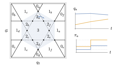
Figure 19: Numerical plots of a trajectory passing from $2_{a}$ to $1_{b}$ (solid line) obtained for large $\eta$ compared with jump location and magnitudes predicted from the exact solution shown in Eq. 70 (broken lines).

Let us now consider the boundary between sectors $2_{a}$ and $1_{b}$ corresponding to the segment

$$\frac{\sqrt{3}q_{2}+q_{1}}{\sqrt{2}}=a,~{}\frac{a}{\sqrt{6}}<q_{2}<\frac{2a}{\sqrt{6}},$$ (63)

shown in Fig. 17 and repeat the steps described above. The energy-momentum relation in the two sectors is

$$E{[2_{a}]} =\frac{1}{2}\left(\left(\pi_{1}^{[2_{a}]}\right)^{2}+3\left(\pi_{2}^{[2_{a}]}\right)^{2}\right),$$

$$E{[1_{b}]} =\frac{1}{4}\left(\sqrt{3}\pi_{2}^{[1_{b}]}-\pi_{1}^{[1_{b}]}\right)^{2}.$$ (64)

The effective eom for $\pi_{\alpha}$ can be obtained by setting $B^{\prime}\left(\frac{\sqrt{3}q_{2}-q_{1}}{\sqrt{2}}\right)=B^{\prime}(\sqrt{2}q_{1})=0$ in Eq. 50 to get

$$\dot{\pi}_{1} =-\frac{\left(\sqrt{3}\pi_{2}+\pi_{1}\right)^{2}}{4\sqrt{2}}B^{\prime}\left(\frac{\sqrt{3}q_{2}+q_{1}}{\sqrt{2}}\right),$$ (65)

$$\dot{\pi}_{2} =-\sqrt{3}\frac{\left(\sqrt{3}\pi_{2}+\pi_{1}\right)^{2}}{4\sqrt{2}}B^{\prime}\left(\frac{\sqrt{3}q_{2}+q_{1}}{\sqrt{2}}\right).$$ (66)

Equations 65 and 66 can be reduced to a single equation

$$\sqrt{3}\dot{\pi}_{1}-\dot{\pi}_{2}=0$$ (67)

Imposing energy conservation and integrating Eq. 67 gives us the following two equations that relates $\pi_{\alpha}^{[2_{a}]}$ and $\pi_{\alpha}^{[1_{b}]}$

$$\frac{1}{2}\left(\left(\pi_{1}^{[2_{a}]}\right)^{2}+3\left(\pi_{2}^{[2_{a}]}\right)^{2}\right) =\frac{1}{4}\left(\sqrt{3}\pi_{2}^{[1_{b}]}-\pi_{1}^{[1_{b}]}\right)^{2},$$

$$\sqrt{3}\pi_{1}^{[2_{a}]}-\pi_{2}^{[2_{a}]} =\sqrt{3}\pi_{1}^{[1_{b}]}-\pi_{2}^{[1_{b}]}.$$ (68)

The sector from which the trajectory is incident decides which momenta in Eq. 68 we consider to be the dependent and independent variables. First, let us consider trajectories incident from the sector $2_{a}$ when $\pi_{\alpha}^{[1_{b}]}$ should be determined in terms of $\pi_{\alpha}^{[2_{a}]}$. From Fig. 19, we see that this requires $\dot{q}^{[2_{a}]}_{2}>0$. From the solution shown in Eq. 55, this condition translates to $\pi_{2}^{[2_{a}]}>0$. Suppose the trajectory enters $1_{b}$. The piecewise solution for the trajectory in sector $1_{b}$ can be determined by rotating Eq. 54 to get

$$q_{1}(t) =q_{1}(0)-~{}\frac{1}{2}~{}\left(\sqrt{3}\pi^{[1_{b}]}_{2}-\pi^{[1_{b}]}_{1}\right)t,$$

$$q_{2}(t) =q_{2}(0)+\frac{\sqrt{3}}{2}\left(\sqrt{3}\pi^{[1_{b}]}_{2}-\pi^{[1_{b}]}_{1}\right)t.$$ (69)

The physical condition for the trajectory entering $1_{b}$, $\dot{q}^{[1_{b}]}_{2}>0$ gives us the condition $\left(\sqrt{3}\pi^{[1_{b}]}_{2}-\pi^{[1_{b}]}_{1}\right)>0$. This picks out the physical solution obtained by solving the quadratic equations in Eq. 68 to give us a unique answer,

$$\pi^{[1_{b}]}_{1}=\frac{3}{2}\pi_{1}^{[2_{a}]} -\frac{\sqrt{3}}{2}\pi_{2}^{[2_{a}]}$$

$$+\frac{1}{\sqrt{2}}\sqrt{\left(\pi_{1}^{[2_{a}]}\right)^{2}+3\left(\pi_{2}^{[2_{a}]}\right)^{2}}$$

$$\pi^{[1_{b}]}_{2}=\frac{\sqrt{3}}{2}\pi_{1}^{[2_{a}]} -\frac{1}{2}\pi_{2}^{[2_{a}]}$$

$$+\sqrt{\frac{3}{2}}\sqrt{\left(\pi_{1}^{[2_{a}]}\right)^{2}+3\left(\pi_{2}^{[2_{a}]}\right)^{2}}.$$ (70)

Equation 70 gives us a valid solution for $\pi_{\alpha}^{[1_{b}]}$ for any physically allowed incident momenta $\pi_{\alpha}^{[2_{a}]}$. As a result, all incident trajectories from $2_{a}$ that strike the $2_{a}-1_{b}$ boundary Eq. 63 pass on to $1_{b}$. Figure 19 shows a sample trajectory confirming the above results.

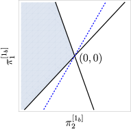
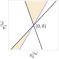
Figure 20: The union of the shaded regions on the left of the dashed line represents the momenta satisfying Eq. 71 for which trajectories starting from $1_{b}$ can strike the boundary with $2_{a}$ (Eq. 63). This is divided into momenta satisfying (left) or not satisfying (right) Eq. 73 for which the trajectories pass on to sector $2_{a}$ or bounce back into sector $1_{b}$ respectively. The solid lines are $2\pi_{1}^{[1_{b}]}+\sqrt{3}\left(1\pm\sqrt{5}\right)\pi_{2}^{[1_{b}]}=0$ and the dashed line is $\sqrt{3}\pi_{2}^{[1_{b}]}=\pi_{1}^{[1_{b}]}$.

We now consider the the case when a trajectory is incident from $1_{b}$. We see from Fig. 21 that such a trajectory requires $\dot{q}^{[1_{b}]}_{2}<0$ which, from Eq. 69 translates to

$$\left(\sqrt{3}\pi^{[1_{b}]}_{2}-\pi^{[1_{b}]}_{1}\right)<0.$$ (71)

This corresponds to the union of the two shaded regions shown in Fig. 20 lying on the left of the dashed line.

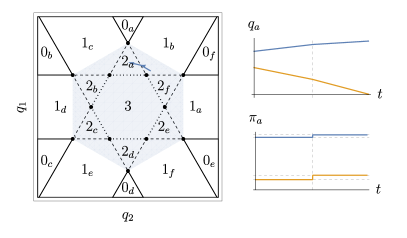
Figure 21: Numerical plots for large $\eta$ (solid lines) of a trajectory passing from $1_{b}$ to $2a$ with initial momenta taking values in the shaded region of the left plot in Fig. 20 compared with jump location and magnitudes predicted from the exact solution shown in Eq. 72 (broken lines).

Let us suppose the trajectory passes through into $2_{a}$, where we require $\dot{q}^{[2_{a}]}_{2}<0$ which imposes $\pi_{2}^{[2_{a}]}<0$. We now solve Eq. 68 to obtain $\pi_{\alpha}^{[2_{a}]}$ in terms of $\pi_{\alpha}^{[1_{b}]}$ subject to these physical conditions to get

$$\pi^{[2_{a}]}_{1}=\frac{9}{10}\pi_{1}^{[1_{b}]}-\frac{3\sqrt{3}}{10}\pi_{2}^{[1_{b}]}$$

$$-\frac{1}{5}\sqrt{3\left(\pi_{2}^{[1_{b}]}\right)^{2}-\left(\pi_{1}^{[1_{b}]}\right)^{2}-\sqrt{3}\pi_{1}^{[1_{b}]}\pi_{2}^{[1_{b}]}},$$

$$\pi^{[2_{a}]}_{2}=-\frac{\sqrt{3}}{10}\pi_{1}^{[1_{b}]}+\frac{1}{10}\pi_{2}^{[1_{b}]}$$

$$-\frac{\sqrt{3}}{5}\sqrt{3\left(\pi_{2}^{[1_{b}]}\right)^{2}-\left(\pi_{1}^{[1_{b}]}\right)^{2}-\sqrt{3}\pi_{1}^{[1_{b}]}\pi_{2}^{[1_{b}]}}.$$ (72)

However, the solutions Eq. 72 are not real-valued for all physical values of $\pi_{\alpha}^{[1_{b}]}$. Real solutions occur when the discriminant is positive definite

$$\left(\pi_{2}^{[1_{b}]}\right)^{2}-\left(\pi_{1}^{[1_{b}]}\right)^{2}-\sqrt{3}\pi_{1}^{[1_{b}]}\pi_{2}^{[1_{b}]}\geq 0.$$ (73)

This reality condition, combined with Eq. 71 tells us for which incident momenta the trajectory can pass from $1_{b}$ to $2_{a}$. This is shown graphically in the left panel of Fig. 20 where the shaded region denotes incident momenta satisfying Eqs. 73 and 71. A sample trajectory satisfying this is presented in Fig. 21.

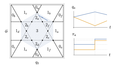
Figure 22: Numerical plots for large $\eta$ (solid lines) of a trajectory incident from $1_{b}$ to the boundary to $2a$ with initial momenta taking values in the shaded region of the right plot in Fig. 20 when the trajectory bounces back to $1_{b}$. The vertical and horizontal broken lines represent the jump location and magnitudes predicted from the exact solution shown in Eq. 76.

For other physical values of $\pi_{\alpha}^{[1_{b}]}$ satisfying Eq. 71 but not Eq. 73 shown in the the shaded region in the right panel of Fig. 20, the trajectory does not go to sector $2_{a}$ but ‘bounces off’ to return to $1_{b}$. Let us denote $\pi_{\alpha<}^{[1_{b}]}$ and $\pi_{\alpha>}^{[1_{b}]}$ to represent the incident and final momenta. The latter can be related to the former using energy conservation $E[1_{b}]_{<}=E[1_{b}]_{>}$ and again using the integrated effective eom Eq. 67 to get the following two equations

$$\frac{1}{4}\left(\sqrt{3}\pi_{2<}^{[1_{b}]}-\pi_{1<}^{[1_{b}]}\right)^{2} =\frac{1}{4}\left(\sqrt{3}\pi_{2>}^{[1_{b}]}-\pi_{1>}^{[1_{b}]}\right)^{2},$$

$$\sqrt{3}\pi_{1<}^{[1_{b}]}-\pi_{2<}^{[1_{b}]} =\sqrt{3}\pi_{1>}^{[1_{b}]}-\pi_{2>}^{[1_{b}]}.$$ (74)

A physical requirement is $\dot{q}^{[1_{b}]}_{2<}<0$ and $\dot{q}^{[1_{b}]}_{2>}>0$ before and after striking the boundary which gives us

$$\left(\sqrt{3}\pi^{[1_{b}]}_{2<}-\pi^{[1_{b}]}_{1<}\right)<0\text{ and }\left(\sqrt{3}\pi^{[1_{b}]}_{2>}-\pi^{[1_{b}]}_{1>}\right)>0.$$ (75)

Solving Eq. 74 subjected to the condition Eq. 75 gives us the unique solution

$$\boxed{\pi^{[1_{b}]}_{1>}=2\pi^{[1_{b}]}_{1<}-\sqrt{3}\pi^{[1_{b}]}_{2<},~{}~{}\pi^{[1_{b}]}_{2>}=\sqrt{3}\pi^{[1_{b}]}_{1<}-2\pi^{[1_{b}]}_{2<}}.$$ (76)

Figure 22 shows such a sample trajectory.

$1_{a}-0_{f}$ boundary

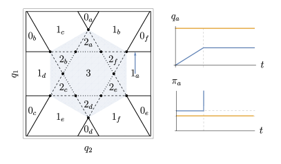
Figure 23: Numerical plots for large $\eta$ of a trajectory incident from $1_{a}$ to the boundary to $0_{f}$. The vertical and horizontal broken lines represent the jump location and magnitudes predicted from the exact solution.

We now consider the boundary between sectors $1_{a}$ and $0_{f}$ corresponding to the semi-infinite line

$$\sqrt{2}q_{1}=a,~{}q_{2}>\sqrt{\frac{3}{2}}a.$$ (77)

The problem is effectively reduced to two-particles considered in Section V.1 and can be solved by regulating the system as discussed in Section V.1. The trajectory can strike the boundary Eq. 77 only if it starts from $1_{a}$ with $\dot{q}_{1}>0$ which, from Eq. 53 translates to $\pi^{[1_{a}]}_{1}>0$. After striking this boundary, the $q_{1}$ becomes motionless and we have the jump $\pi_{1}\rightarrow\infty$. $q_{2}(t)=q_{2}(0)$ throughout and does not change. A sample trajectory is shown in Fig. 23.

$3-2_{e}-2_{f}-1_{a}$ junction

We now look at the points in Fig. 17 where more than two sectors meet beginning with the point

$$\left(\tilde{q}_{1},\tilde{q}_{2}\right)=a\left(0,\sqrt{\frac{2}{3}}\right)$$ (78)

where sectors $3,2_{e},2_{f}$ and $1_{a}$ meet. First, let us look at the effective eom for $\pi_{\alpha}$. Since the point $(\tilde{q}_{1},\tilde{q}_{2})$ is where the lines $\sqrt{3}q_{2}\pm q_{1}=\sqrt{2}a$ meet, we have $B^{\prime}\left(\sqrt{2}q_{1}\right)=0$ and $B^{\prime}\left(\frac{\sqrt{3}\tilde{q}_{2}+\tilde{q}_{1}}{\sqrt{2}}\right)=B^{\prime}\left(\frac{\sqrt{3}\tilde{q}_{2}-\tilde{q}_{1}}{\sqrt{2}}\right)$ in the trajectory that goes through this point. Using this in Eq. 50, we get

$$\dot{\pi}_{1} =-\sqrt{\frac{3}{2}}\pi_{1}\pi_{2}~{}B^{\prime}\left(\frac{\sqrt{3}\tilde{q}_{2}\pm\tilde{q}_{1}}{\sqrt{2}}\right),$$

$$\dot{\pi}_{2} =-\frac{1}{2}\sqrt{\frac{3}{2}}\left(3\pi_{2}^{2}+\pi_{1}^{2}\right)~{}B^{\prime}\left(\frac{\sqrt{3}\tilde{q}_{2}\pm\tilde{q}_{1}}{\sqrt{2}}\right).$$ (79)

This can be massaged to give us

$$\left(3\pi_{2}^{2}+\pi_{1}^{2}\right)\dot{\pi}_{1}=2\pi_{1}\pi_{2}\dot{\pi}_{2}\implies\frac{d}{dt}\left(\frac{\pi_{1}^{2}+\pi_{2}^{2}}{\pi_{1}^{3}}\right)=0.$$ (80)

The integrated version of Eq. 80 together with energy conservation would give us the two equations which we can solve to determine the jump condition for a trajectory that touches the point $(\tilde{q}_{1},\tilde{q}_{2})$ shown in Eq. 78. From the solution for the trajectory in $1_{a}$ shown in Eq. 54, we see that motion only occurs perpendicular to the extended direction in this sector. This allows no possibility for the trajectory to either be incident or pass onto $1_{a}$. Thus, the only trajectories that can strike Eq. 78 are those confined to sectors $3$ or $2_{e,f}$.

$2_{a}-1_{b}-1_{c}-0_{a}$ junction

Finally, we look at the point

$$\left(\tilde{q}_{1},\tilde{q}_{2}\right)=a\left(\sqrt{2},0\right)$$ (81)

where sectors $2_{a},1_{b},1_{c}$ and $0_{a}$ meet. Since this is where the lines $\sqrt{3}q_{2}\pm q_{1}=\sqrt{2}\pm a$ meet, we have $B^{\prime}\left(\sqrt{2}q_{1}\right)=0$ and $B^{\prime}\left(\frac{\sqrt{3}\tilde{q}_{2}+\tilde{q}_{1}}{\sqrt{2}}\right)=B^{\prime}\left(\frac{\sqrt{3}\tilde{q}_{2}-\tilde{q}_{1}}{\sqrt{2}}\right)$ for trajectories that strike this point giving us the same condition shown in Eq. 80. This, along with conservation of energy will give us the two equations to determine jump conditions. Since there is no motion in sector $0_{a}$, trajectories striking this point are restricted to $2_{a}$ and $1_{b-c}$.

Jump conditions for trajectories striking line-line boundaries required us to solve quadratic equations for which we have presented exact solutions. The jump conditions for trajectories that strike the two classes of point-like boundaries described above requires us to solve cubic equations arising from Eq. 80 along with the quadratic equations from the conservation of energy. This too can be done exactly in principle to determine the various possible bounce and pass-through scenarios. We will however not do this explicitly since we feel it would not add much to the discussion.

V.5 Sample trajectory and discussion

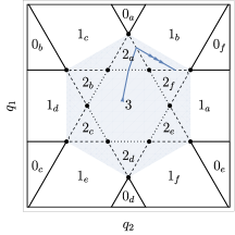
Figure 24: Numerical plots of a sample trajectory starting from the central sector $3$. The broken lines represent the theoretically determined values between which the full trajectory interpolates.

Let us put all these together to understand a sample trajectory shown in Fig. 24 obtained numerically (shown in thick lines). Here, the trajectory begins in sector $3$ and settles down to an indefinite oscillation in sector $1_{b}$, while the momenta grow large indefinitely, consistent with the picture in Fig. 10. We mark the various locations where the trajectory crosses sectors along with associated momentum jump values using broken lines.

From the piecewise solution, we see that for any initial condition starting anywhere within the shaded region in Figs. 17 and 24, the trajectory never leaves the region. And conversely any initial condition located outside the shaded region never enters the shaded region effectively dividing all trajectories. The latter class always ends on the border between some $0_{\alpha}$ and $1_{\beta}$ sectors when the position coordinate becomes frozen and momentum diverges. On the other hand, we observe that without fine-tuning, generic initial conditions starting anywhere within the shaded region in Figs. 17 and 24 end up in such oscillatory steady states in the triangular shaded slivers in any one of the sectors $1_{a-f}$ of the form shown in Fig. 24. The asymptotic oscillations correspond to the trajectory repeatedly bouncing between two borders separating some $1_{\beta}$ sector with adjacent $2_{\alpha}$ sectors.

VI Phase space fragmentation and ergodicity breaking

We now discuss specific aspects of the fracton dynamics listed in Sections III and V and also make contact with known quantum fracton phenomenology explored in previous work [15, 16, 9, 10, 14, 22, 23].

VI.1 Asymptotic conserved quantities and phase space fragmentation

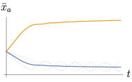
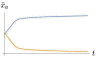
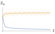
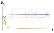
Figure 25: Fragmentation of the total center of mass in a single cluster into asymptotically conserved centres of mass for particles in each cluster (thick lines) for the particle trajectories shown in Figs. 10 and 13 (thin, dashed lines).

Fractonic trajectories exhibit emergent and asymptotic symmetries and conserved quantities. This was briefly mentioned in passing in Sections III and V and we will now discuss it in detail. Emergent conservation laws appear in two distinct ways as a consequence of the interplay between dipole conservation and locality. The first is more direct and determined largely by initial conditions. Recall the discussion in Fig. 3 where we argued that for initially far-separated particles, the dynamics generated by the Hamiltonian in Eq. 20 not only conserves the total dipole moment but also individual particle position coordinates. In other words, the total conserved dipole moment has fragmented into $N$ parts. We will use the symbol $\rightsquigarrow$ to denote the fragmentation of charge as follows

$$\sum_{a}x_{a}\rightsquigarrow\{x_{a}\}.$$ (82)

This directly generalizes to the case when particles start off in $P$ well-separated Machian clusters $\mathcal{M}_{1},\ldots,\mathcal{M}_{P}$. We expect local dipole conserving dynamics to prevent particles from moving between clusters and as a result, the dipole moment of particles within each Machian cluster $\mathcal{M}_{p}$ is independently conserved,

$$\sum_{a}x_{a}\rightsquigarrow\{\sum_{a\in\mathcal{M}_{p}}x_{a}\}.$$ (83)

A second, less direct way emergent conservation laws appear is when particles start off within a single Machian cluster and asymptotically separate into multiple adjacent clusters. Let us consider the fractonic trajectories of two particles with close initial separation shown in Fig. 5. Here, we see that at late times, not just the total dipole moment of the two particles in the cluster but the coordinate of each individual particle is a conserved quantity

$$x_{1}+x_{2}\rightsquigarrow\{x_{1},x_{2}\}.$$ (84)

This generalizes to the fractonic trajectories for three and four particles shown in Figs. 10 and 13. At late times, the particles separate into two subsystems with each undergoing different possible asymptotic dynamics. Regardless of the nature of this dynamics, we see that asymptotically, the dipole moment (centre of mass) of each subsystem is independently conserved and becomes constant in time. The precise nature of how the total dipole moment is fragmented depends sensitively on the initial conditions, and can take one of the following forms

$$\sum_{a=1}^{3}x_{a}\rightsquigarrow\text{permutations of}~{}\{x_{1},x_{2}+x_{3}\}$$ (85)

$$\sum_{a=1}^{4}x_{a}\rightsquigarrow\text{permutations of}~{}\begin{cases}\{x_{1}+x_{2},x_{3}+x_{4}\}\\ \{x_{1},x_{2}+x_{3}+x_{4}\}\end{cases}$$ (86)

Figure 25 reproduces the trajectories shown in Figs. 10 and 13 (dashed lines) along with the emergent conserved centres of masses $\bar{x}_{a}$ (thick lines). For a larger number of particles, we observe a similar phenomenon. However, the precise number of asymptotic clusters is hard to determine because it is hard to conclusively establish that seemingly stable clusters will not interact by exchanging particles at very long timescales. We will not discuss this further in this work.

VI.2 Ergodicity breaking and the failure of statistical mechanics

In the study of equilibrium many-body physics an important role is played by ergodicity and its breaking [24]. Unbroken ergodicity allows us to relate physically relevant time-averaged observables, $\overline{O(\{x_{j},p_{j}\})}$ with with calculationally convenient ensemble-averaged ones $\langle O(\{x_{j},p_{j}\})\rangle$ which is the subject of statistical mechanics. The latter is computed by averaging the observable over all phase space available to the system, $\Gamma$. When ergodicity is broken, the system does not explore all available phase space but gets stuck in distinct sectors $\Gamma\rightsquigarrow\{\Gamma_{\alpha}\}$. In certain situations, when $\Gamma_{\alpha}$ can be well-enumerated, statistical mechanics can still be used by appropriately restricting the ensemble to $\Gamma_{\alpha}$, using appropriate bias fields or chemical potentials. This is the case when ergodicity breaking occurs through spontaneous symmetry breaking where the sectors $\Gamma_{\alpha}$ are labelled by elements of the coset $\alpha\in G/H$ of unbroken ($G$) and residual ($H$) symmetries. A dilute gas of dipole conserving systems undergoing fractonic trajectories exhibits ergodicity breaking of a different kind. Here, the nature of the restricted phase space $\Gamma_{\alpha}$ in which the system becomes trapped depends on the initial conditions and cannot be easily accommodated within statistical mechanics.

This occurs through two possible mechanisms discussed above in Section VI.1. The first involves particles starting in distant Machian clusters $\mathcal{M}_{\alpha}$ which do not merge under dynamics resulting in the system exploring only a fraction of symmetry-allowed phase space. The second is the asymptotic fragmentation of particles starting under close separation into multiple sub-clusters that was seen in Sections III and IV. Whether the latter phenomenon is a feature of small number of particles or survives in a many-body setting, perhaps in a low-density limit, is an open question for future investigation. At high densities, we may expect that most initial conditions leads to several particles starting out in a single cluster. In this case, either the system might restore ergodicity beyond some critical density leading to a orthonormalization transtion as seen in studies of quantum systems [22, 14]. Another possibility is that asymptotic sub-cluster formation persists and presents a barrier to the restoration of ergodicity even at high densities. This is another open question for future work.

VII Relation to quantum fractons

For most of this paper, we have used words such as ‘fractons’ without making reference to the quantum mechanical systems and phases of matter whence the name was coined. We now draw comparisons between the phenomena studied in this work and those that are well known for quantum fractons

VII.1 Topological phases, gauging and dipole conservation

To keep our work self-contained, we now provide a brief review of quantum fractons and the relation to multipole conserving systems. Readers who are familiar with these can skip ahead to the next subsection. We also direct readers who are interested in more details to other dedicated reviews [1, 2].

The term fractons originally referred to the quasi-particle excitations in a recently discovered class of gapped phases of quantum matter [5, 3, 25]. These excitations were found to have restricted mobility and were constrained to move along sub-dimensional manifolds such as planes, lines [26] or fractals [3]. Fracton phases are ‘topologically ordered’ [27] in the sense that they are absolutely stable [28] to arbitrary local perturbations [29]. An important conceptual tool in studying such phases is gauging – if we start with a system with an unbroken on-site global symmetry and dynamically gauge it i.e. elevate it to a local redundancy structure, we get a topologically ordered system [30] belonging to the deconfined phase of the gauge theory. It was shown [26, 6, 2, 7] that fracton topological order too can be be obtained by starting with systems with an unbroken global multipole conservation symmetry and dynamically gauging it.

Interestingly, ‘ungauged’ systems with exact global multipole symmetry were found to host a variety of interesting phenomena found in the gauged counter parts and beyond:

1. Their gapped excitations also have restricted mobility [6].

2. They exhibit Hilbert space fragmentation characterized by a large number of emergent symmetries and conserved quantities [15, 23, 16].

3. Their dynamics is ‘glassy’ i.e. anomalously slow [5].

4. They exhibit ‘UV-IR mixing’ – a phenomena where long-distance (IR) behaviour is not completely divorced of its microscopic (UV) details [31, 9, 10].

On the one hand, without gauging, these properties are no longer absolutely stable and are conditional on the presence of exact microscopic multipole symmetries. On the other hand, models with exact symmetries are easier to construct and study and this is the spirit of this work too.

VII.2 Classical and quantum fractons - similarities and differences

Restricted mobility: We begin with the most iconic piece of fracton phenomenology– particles with restricted mobility. In quantum mechanical models [25], excitations of like charges are completely immobile whereas composites of charge-neutral dipoles have restricted mobility. We see both of these reflected in classical dynamics shown in Section III. The latter is evident from the vanishing of the Hamiltonian Eq. 20 for well-separated particles whereas the former is seen in the dynamics of unlike particles shown in Section IV.1. The dynamics of like particles at close separation, shown in Sections III and V however, to the best of our knowledge have no counterpart studied in exactly solvable models [3, 25, 26, 5] or in continuum field theories [9, 6, 8]. The dynamics shown in Sections III and V correspond to short-distance core dynamics of small clusters of particles that are not naturally captured by fixed-point or continuum models. If we consider realistic models with finite correlation length or actual experimental systems, we expect this dynamics (or quantum versions thereof) to be present at low densities of fractons.

Hilbert space fragmentation and ergodicity breaking: In Refs.[15, 16] it was observed that quantum dynamics preserving dipole moment results in a fragmentation of Hilbert space– the space of states carrying the same symmetry quantum numbers were found to organize themselves into dynamically disconnected distinct Krylov sectors. The size and nature of these Krylov sectors were found to depend on the locality of the Hamiltonian that generates dynamics. In our classical systems, we discussed that initial conditions separates the particles into distinct Machian clusters which do not merge under dynamics. These disconnected Machian clusters resulting in phase-space fragmentation are direct classical analogues of Krylov subspaces. However, we also saw that particles starting within a single Machian cluster can asymptotically separate into distinct ones resulting in further phase space fragmentation that are not easily determined from initial conditions. To the best of our knowledge, there is no known quantum analog of this asymptotic fragmentation.

For a low density of particles, the typical size of the Krylov subspace is a vanishing fraction of the total Hilbert space allowed by symmetry and therefore the system violates the eigenstate thermalization hypothesis [32] therefore breaking ergodicity, similar to the classical case discussed in Section VI.1. Recently, Refs. [22, 14] explored an interesting possibility– by tracking the size of the largest Krylov subspace relative to the size of the symmetry sector, the authors showed that the system that breaks ergodicity at low densities can restore it at higher densities undergoing a sharp transition at a critical density whose critical properties can be determined. We can envision the possibility of such a transition in the classical setting too. However, as previously discussed, it is unclear whether the emergence of asymptotic fragmentation observed even for closely separated particles persists for larger numbers and introduces a new barrier to thermalization even at high densities.

Figure 26: Energy contours for the two-particle system shown in Eq. 88 with $a=1,\eta=10$. Observe that the hypersurfaces are unbounded in the momentum direction and therefore the usual association between energy and momentum scales no longer holds.

UV-IR mixing: A general expectation from generic many-body phases is that short-distance (UV) properties of the system on the scale of lattice spacing should not affect long-distance (IR) properties. This allows the use of renormalization group techniques and approximate continuum models for analysis. Long-distance properties of systems with multipole conservation and fracton topological order are known to be sensitive to UV details (such as the lattice structure) and are not easily amenable to analysis using continuum and RG methods. This has been dubbed UV-IR mixing [31, 9, 10]. One of the ways in which UV-IR mixing manifests itself is in the disassociation between the magnitudes of energy and momenta. We can see classical equivalents of this in the way constant energy hypersurfaces foliate phase space for dipole conserving systems. Recall that for ordinary i.e. dipole non-conserving systems, momentum space projections of constant energy hypersurfaces take the form of spheres whose radius indicates the energy of the system

$$\sum_{a}|\vec{p}_{a}|^{2}\sim 2mE.$$ (87)

This naturally leads to an association of the momentum scales with energy. For dipole conserving systems on the other hand, this is no longer true. Consider the two-particle dipole conserving system without interactions, written in reduced coordinates

$$E=\pi_{1}^{2}K(\sqrt{2}q_{1}).$$ (88)

Constant energy surfaces of Eq. 88 are shown in Fig. 26. Fractonic trajectories Fig. 5 appear as open surfaces that are unbounded in the momentum direction. Energy and momentum scales are now no longer related.

VIII Conclusions and future directions

In this work, we studied non-relativistic fractons – point-particle systems with dipole conservation. Using numerical calculations, we show that the classical mechanics of finite number of fractons exhibits several unusual and novel features – velocity, energy, momentum mismatch, asymptotic steady-state dynamics in the form of attractors and limit cycles seemingly inconsistent with Liouville’s theorem, emergent conserved quantities and dynamical fragmentation. We also presented an exact solution for the three-particle system using a certain limiting Hamiltonian form.

There are several extensions of this work involving quantization, many-particles, higher dimensions, higher multipole conservations and combinations thereof which are interesting to explore. First, it would be interesting to extend our analysis to higher dimensions where more possibilities emerge. The allowed form of the locality term $K$ can take various forms and different choices can lead to distinct classes of Machian dynamics. It would also be illuminating to canonically quantize the few-particle system and see to what extent and in what ways, if at all the classical features discussed in this work are manifested. As discussed in Section VI.1, it would be interesting to see if the many-fracton system restores ergodicity at some critical value of particle or energy density and in what ways it is similar to or different from a similar transition that is known to occur in quantum many-fracton systems on the lattice [22, 14]. Finally, it would also be interesting to see if a continuum description can be given using our starting point to make contact with field theoretic [9] and hydrodynamic studies [7]. We leave these and other questions to future work.

References

- Nandkishore and Hermele [2019] R. M. Nandkishore and M. Hermele, Fractons, Annual Review of Condensed Matter Physics 10, 295 (2019), https://doi.org/10.1146/annurev-conmatphys-031218-013604 .
- Pretko et al. [2020] M. Pretko, X. Chen, and Y. You, Fracton phases of matter, International Journal of Modern Physics A 35, 2030003 (2020).
- Haah [2011] J. Haah, Local stabilizer codes in three dimensions without string logical operators, Phys. Rev. A 83, 042330 (2011).
- Note [1] Once fractons were excitations on a fractal background sciencedirect.com/science/article/pii/0167278989902042 but that copyright expired a while back.
- Chamon [2005] C. Chamon, Quantum glassiness in strongly correlated clean systems: An example of topological overprotection, Phys. Rev. Lett. 94, 040402 (2005).
- Pretko [2018] M. Pretko, The fracton gauge principle, Phys. Rev. B 98, 115134 (2018).
- Gromov [2019] A. Gromov, Towards classification of fracton phases: The multipole algebra, Phys. Rev. X 9, 031035 (2019).
- Pretko [2017] M. Pretko, Emergent gravity of fractons: Mach’s principle revisited, Phys. Rev. D 96, 024051 (2017).
- Gorantla et al. [2021] P. Gorantla, H. T. Lam, N. Seiberg, and S.-H. Shao, Low-energy limit of some exotic lattice theories and uv/ir mixing, Phys. Rev. B 104, 235116 (2021).
- You and Moessner [2022] Y. You and R. Moessner, Fractonic plaquette-dimer liquid beyond renormalization, Phys. Rev. B 106, 115145 (2022).
- Mach [1907] E. Mach, The science of mechanics (Prabhat Prakashan, 1907).
- Barbour and Pfister [1995] J. B. Barbour and H. Pfister, Mach’s principle: from Newton’s bucket to quantum gravity, Vol. 6 (Springer Science & Business Media, 1995).
- Bondi and Samuel [1997] H. Bondi and J. Samuel, The lense-thirring effect and mach’s principle, Physics Letters A 228, 121 (1997).
- Pozderac et al. [2023] C. Pozderac, S. Speck, X. Feng, D. A. Huse, and B. Skinner, Exact solution for the filling-induced thermalization transition in a one-dimensional fracton system, Phys. Rev. B 107, 045137 (2023).
- Khemani et al. [2020] V. Khemani, M. Hermele, and R. Nandkishore, Localization from hilbert space shattering: From theory to physical realizations, Phys. Rev. B 101, 174204 (2020).
- Sala et al. [2020] P. Sala, T. Rakovszky, R. Verresen, M. Knap, and F. Pollmann, Ergodicity breaking arising from hilbert space fragmentation in dipole-conserving hamiltonians, Phys. Rev. X 10, 011047 (2020).
- Lynden-Bell and Katz [1995] D. Lynden-Bell and J. Katz, Classical mechanics without absolute space, Phys. Rev. D 52, 7322 (1995).
- [18] Wolfram Research, Inc, Mathematica, Version 13.2, champaign, IL, 2023.
- Strogatz [2018] S. H. Strogatz, Nonlinear dynamics and chaos with student solutions manual: With applications to physics, biology, chemistry, and engineering (CRC press, 2018).
- Hénon and Heiles [1964] M. Hénon and C. Heiles, The applicability of the third integral of motion: some numerical experiments, Astronomical Journal, Vol. 69, p. 73 (1964) 69, 73 (1964).
- Ramond [2010] P. Ramond, Group Theory: A Physicist’s Survey (Cambridge University Press, 2010).
- Morningstar et al. [2020] A. Morningstar, V. Khemani, and D. A. Huse, Kinetically constrained freezing transition in a dipole-conserving system, Phys. Rev. B 101, 214205 (2020).
- Moudgalya et al. [2022] S. Moudgalya, B. A. Bernevig, and N. Regnault, Quantum many-body scars and hilbert space fragmentation: a review of exact results, Reports on Progress in Physics 85, 086501 (2022).
- Palmer [1982] R. Palmer, Broken ergodicity, Advances in Physics 31, 669 (1982), https://doi.org/10.1080/00018738200101438 .
- Vijay et al. [2015] S. Vijay, J. Haah, and L. Fu, A new kind of topological quantum order: A dimensional hierarchy of quasiparticles built from stationary excitations, Phys. Rev. B 92, 235136 (2015).
- Vijay et al. [2016] S. Vijay, J. Haah, and L. Fu, Fracton topological order, generalized lattice gauge theory, and duality, Phys. Rev. B 94, 235157 (2016).
- Wen [1990] X.-G. Wen, Topological orders in rigid states, International Journal of Modern Physics B 4, 239 (1990).
- von Keyserlingk et al. [2016] C. W. von Keyserlingk, V. Khemani, and S. L. Sondhi, Absolute stability and spatiotemporal long-range order in floquet systems, Phys. Rev. B 94, 085112 (2016).
- Bravyi et al. [2010] S. Bravyi, M. B. Hastings, and S. Michalakis, Topological quantum order: Stability under local perturbations, Journal of Mathematical Physics 51, 093512 (2010).
- Levin and Gu [2012] M. Levin and Z.-C. Gu, Braiding statistics approach to symmetry-protected topological phases, Phys. Rev. B 86, 115109 (2012).
- Minwalla et al. [2000] S. Minwalla, M. V. Raamsdonk, and N. Seiberg, Noncommutative perturbative dynamics, Journal of High Energy Physics 2000, 020 (2000).
- Deutsch [2018] J. M. Deutsch, Eigenstate thermalization hypothesis, Reports on Progress in Physics 81, 082001 (2018).