Isolating Dust and Free-Free Emission in ONC Proplyds with ALMA Band 3 Observations

Abstract

The Orion Nebula Cluster (ONC) hosts protoplanetary disks experiencing external photoevaporation by the cluster’s intense UV field. These “proplyds” are comprised of a disk surrounded by an ionization front. We present ALMA Band 3 (3.1 mm) continuum observations of 12 proplyds. Thermal emission from the dust disks and free-free emission from the ionization fronts are both detected, and the high-resolution (0$\farcs$057) of the observations allows us to spatially isolate these two components. The morphology is unique compared to images at shorter (sub)millimeter wavelengths, which only detect the disks, and images at longer centimeter wavelengths, which only detect the ionization fronts. The disks are small ($r_{d}$ = 6.4–38 au), likely due to truncation by ongoing photoevaporation. They have low spectral indices ($\alpha\lesssim 2.1$) measured between Bands 7 and 3, suggesting the dust emission is optically thick. They harbor tens of Earth masses of dust as computed from the millimeter flux using the standard method, although their true masses may be larger due to the high optical depth. We derive their photoevaporative mass-loss rates in two ways: first, by invoking ionization equilibrium, and second using the brightness of the free-free emission to compute the density of the outflow. We find decent agreement between these measurements and $\dot{M}$ = 0.6–18.4 $\times$ 10^-7 $M_{\odot}$ yr^-1. The photoevaporation timescales are generally shorter than the $\sim$1 Myr age of the ONC, underscoring the known “proplyd lifetime problem.” Disk masses that are underestimated due to being optically thick remains one explanation to ease this discrepancy.

1 Introduction

The Orion Nebula Cluster (ONC) provides an ideal site to study star and planet formation in a cluster environment. Clusters are where most stars and planets form (Lada & Lada, 2003), and evidence suggests our solar system formed in a cluster (Adams, 2010). The ONC comprises thousands of 1–2 Myr old stars (Fang et al., 2021) and resides at a distance of $\sim$400 pc (Jeffries, 2007; Menten et al., 2007; Kounkel et al., 2017). Unlike low-mass star-forming regions (e.g., Taurus-Auriga, $\rho$ Ophiuchus, Lupus, Chamaeleon, etc.), clusters host luminous OB stars, which irradiate their surroundings with UV photons. In the ONC, these are the Trapezium stars, most notably the O7V (binary) star $\theta^{1}$Ori C (Sota et al., 2011).

The high-UV environment is expected to heat and photoevaporate protoplanetary disks around young stars in the cluster, driving mass loss via a wind and truncating the disks’ radii (Johnstone et al., 1998; Störzer & Hollenbach, 1999; Adams et al., 2004; Clarke, 2007; Winter et al., 2018; Sellek et al., 2020; Marchington & Parker, 2022; Winter & Haworth, 2022). This impacts the physical and chemical properties of the disks (Walsh et al., 2013; Boyden & Eisner, 2023) and the planet formation process occurring within (Throop & Bally, 2005; Haworth et al., 2018; Winter et al., 2022; Qiao et al., 2023). Observations of the ONC with the Atacama Large Millimeter/submillimeter Array (ALMA) found a deficit of large disks compared with low-mass star-forming regions, providing evidence for disk truncation by photoevaporation (Eisner et al., 2018; Boyden & Eisner, 2020; Otter et al., 2021; Boyden & Eisner, 2023). However, other mechanisms, such as dynamical encounters and interstellar medium (ISM) interactions (Wijnen et al., 2017) or higher cosmic-ray ionization (Kuffmeier et al., 2020), could also explain the small disk sizes in clusters like the ONC.

Direct evidence for ongoing external photoevaporation is provided by the proplyds—disks surrounded by an ionization front with a comet-like morphology. The external UV field heats the disks, driving material off in a photoevaporative wind. In most observed proplyds, the wind is neutral and driven by far-UV (FUV), rather than extreme-UV (EUV), photons. The outflowing material eventually encounters ionizing photons, mostly from $\theta^{1}$Ori C, yielding the observable ionization front that is well separated from the outer edge of the disk. Proplyds have recently been discovered in other star-forming regions (Kim et al., 2016; Haworth et al., 2021) although the ONC remains the site of the majority of known proplyds.

The morphology of proplyds was first observed in Hubble Space Telescope (HST) images of the ONC by O’dell et al. (1993), and proplyds have been targeted with numerous HST observations since (O’dell & Wen, 1994; O’dell & Wong, 1996; Bally et al., 1998a, 2000; Ricci et al., 2008).

At centimeter wavelengths, the free-free emission from proplyd ionization fronts was detected with the Very Large Array (VLA; Churchwell et al., 1987). While the sources were slightly extended, their morphology was not clearly visible in these early radio observations. More recent observations with the VLA did reveal the structure of many ONC proplyds at centimeter wavelengths (Forbrich et al., 2016; Sheehan et al., 2016), although neither of these studies performed an analysis of proplyd morphology.

Early (sub)millimeter observations were only sensitive enough to detect the brightest ONC sources and lacked the spatial resolution to image proplyds in detail (Mundy et al., 1995; Bally et al., 1998b; Williams et al., 2005; Eisner & Carpenter, 2006). ALMA offered a significant improvement in both sensitivity and resolution, with observations of the ONC at Band 6 (1.3 mm; Eisner et al., 2016) and Band 7 (0.86 mm; Mann et al., 2014; Eisner et al., 2018) detecting many sources, including proplyds. However, at these wavelengths the extended free-free emission from the ionization fronts was not seen; the observations instead detected compact sources arising from dust in the protoplanetary disks.

Here we present ALMA Band 3 (3.1 mm) observations of the ONC, focusing on 12 proplyd systems. At this wavelength, ALMA is sensitive to both dust emission from the disk and free-free emission from the ionization front. With a resolution of 0$\farcs$057, these observations can spatially resolve these two components, allowing each to be characterized independently.

2 Methods

2.1 ALMA Band 3 Observations

ALMA Band 3 observations of the ONC were performed in Cycle 6 project 2018.1.01107.S. The ONC was mosaicked with ten pointings, labeled Field IDs 5–14. Four observation blocks were carried out, the first (observation ID 0) on 2019 July 7 and the remaining three (observation IDs 1, 2, and 3) on 2019 July 9. The C43-9 configuration was used with 43 antennas in observations 0, 2, and 3, and 45 antennas in observation 1. Four spectral windows were used with central frequencies of 90.5, 92.4, 102.5, and 104.4 GHz. Each spectral window had a bandwidth of 1.875 GHz sampled with 1920 channels. Separate spectral window IDs were assigned for each of the four observations, resulting in 16 total spectral window IDs labeled 0–15.

We began our reduction with the pipeline-calibrated measurement set. Because we are only interested in the continuum, we flagged channels exhibiting line emission. This was done by inspecting the amplitude versus channel plot of each spectral window for each field. We then spectrally averaged the data with a bin width of 128 channels to produce a continuum measurement set with 15 channels per spectral window.

These observations detect many sources, necessitating analysis of the image plane rather than of the visibilities directly. We imaged the continuum with the CASA task tclean in multi-frequency synthesis (mfs) mode. All ten fields were imaged together using the mosiac gridder with a phase center at 05:35:16.578 $-$05:23:12.150. The pixel size is 0$\farcs$008 and the image size is 19,600 $\times$ 22,500 pixels (2$\farcm$6 $\times$ 3$\arcmin$), which includes a signal-free buffer region around the mosaic. The region of the mosaic with signal spans 05:35:11.71 to 05:35:21.45 in R.A. and $-$05:21:48.5 to $-$05:24:35.8 in decl. although it does not completely fill this rectangle, and the signal-to-noise ratio is poor near the edges. The footprint of the mosaic on an HST image is shown in Figure 1. The mtmfs deconvolver was used with point-source model components and two spectral terms. Briggs weighting was used with a robust parameter of 0.5, resulting in a beam size of 0$\farcs$057 $\times$ 0$\farcs$072 (23 $\times$ 29 au at 400 pc). This resolution is comparable to the famous HST images of proplyds in the optical (e.g., 0$\farcs$05; Bally et al., 1998a). We also imaged the mosaic a second time with a robust parameter of 2.0, yielding a beam size of 0$\farcs$069 $\times$ 0$\farcs$107 (28 $\times$ 43 au). This image has lower spatial resolution but higher sensitivity to extended emission.

Upon initially imaging the data from the four observations combined, we noticed persistent artifacts surrounding some of the brightest sources, most notably $\theta^{1}$ Ori A. We found the artifacts are due in part to source variability. Similar imaging artifacts were seen around $\theta^{1}$ Ori A in VLA observations (Forbrich et al., 2016). To address this, we first modeled the three brightest sources in the mosaic—$\theta^{1}$ Ori A, BN, and Source I—for each observation separately and used the CASA task uvsub to subtract this model from the data before imaging all observations together. This effectively removed these sources, and their artifacts, from the final image.

We self-calibrated the data during the initial per-observation imaging of the three bright sources. We derived and applied two iterations of phase calibration solutions for each field individually and thus to only the fields containing signal from these three sources. This resulted in modestly higher S/N in these fields.

The final imaging was performed with the automasking capabilities of the tclean task (using the “auto-multithresh” algorithm) to generate clean masks around sources in the mosaic. After some experimentation, we found that a side-lobe threshold value of 1.5 and a noise threshold value of 4.5 worked well to identify and clean most observable sources while converging relatively quickly. Lastly, we corrected the mosaic for the response of the primary beam using the widebandpbcor task.

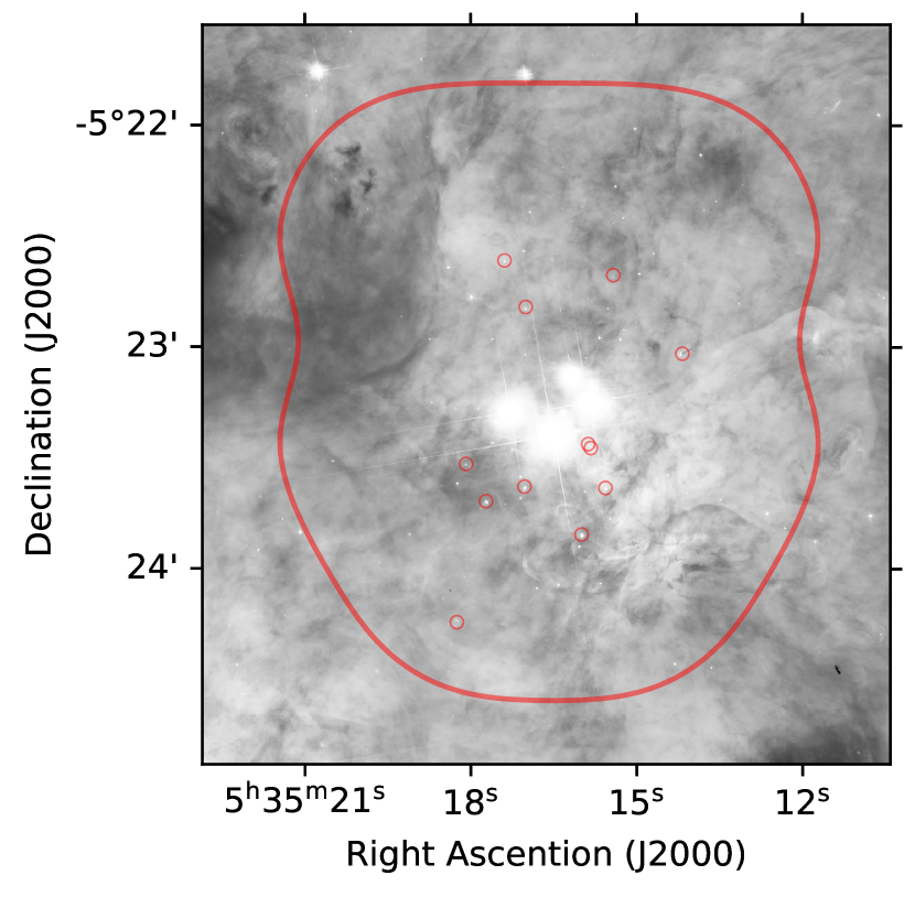
Figure 1: HST/Advanced Camera for Surveys F435W image of the ONC center by Robberto et al. (2013) overlaid with the field of view of the ALMA Band 3 mosaic and the locations of the 12 proplyds presented in this paper (red circles). The bright Trapezium stars are visible in the center of the image. North is up, and East is left.

2.2 Supplementary Data

To obtain a multiwavelength picture of our sources, we also acquired the ALMA Band 7 (0.86 mm) image of the ONC published by Eisner et al. (2018) and the VLA images at $K$ (1.3 cm), $X$ (3.6 cm), and $C$ (6 cm) Bands published by Sheehan et al. (2016).

2.3 Source Identification and Measurements

We identify over 200 sources in our final Band 3 mosaic. In this paper we focus only on the 12 proplyd systems that clearly exhibit both compact emission from a disk and free-free emission in a comet-like structure. An analysis of the full sample will be presented in future work. These 12 sources are well-known proplyds from HST images, and their locations are marked in Figure 1. We refer to the proplyds by the six-digit coordinate-based naming scheme introduced by O’dell & Wen (1994), where the name XXX-YYY corresponds to a source in a $1\farcs 5\times 1\arcsec$ box whose northwest corner is at R.A. of 5:35:XX.X and decl. of -5:2Y:YY. In Figures 2, 3, and 4 we show the submillimeter through centimeter morphology of these proplyds.

To measure the disk component of each proplyd, we fit a 2D Gaussian to the central source using the CASA task imfit. Including a zero level offset in the fit yielded residuals with minimal structure aside from the expected free-free extended emission. The disk coordinates, deconvolved size, PA, and total flux density of each source are reported in Table 1. All 12 disks were successfully deconvolved in this manner. Additional properties of these systems, derived from the measurements, are presented in Table 2.

We measure the Band 7 flux densities of these sources using imfit as well, and we report the results in Table 1. Eisner et al. (2018) measured Band 7 flux densities from the same data using the peak surface brightness rather than Gaussian fitting. To ensure a consistent measurement approach when comparing Band 7 and Band 3 (Section 3.4), we opt to use only the Band 7 values measured with imfit. These are typically higher than the fluxes reported by Eisner et al. (2018), especially for the larger sources. We lack Band 7 measurements for one source, 182-413, because it resides outside the Band 7 mosaic.

We generate surface brightness cuts along and across the proplyds, as shown in Figure 5. Each cut is from a 9 pixel (0$\farcs$072) wide strip centered on the disk. We made the cuts from the Band 3 (r=0.5) images after rotating them so the proplyd head faced up. Each head-to-tail cut (blue line) shows a prominent peak from the disk and a secondary peak at positive separations arising from the ionization front with brightness and width that varies considerably among the sources. For some of the sources (e.g., 155-38, 158-326, and 158-327) flux from the proplyd tail can also be seen in these cuts at negative values. The left-to-right cuts (red lines) show the disk and, in some sources, the sides of the ionization front.

We measure the size of the ionization front, which can be used to infer the photoevaporative mass-loss rate, as we will discuss is Section 3.6. Specifically, we measure $r_{\text{IF}}$, the distance from the disk center to the outer edge of free-free emission along the direction directly away from the proplyd tail. We do so using the surface brightness cuts, specifying $r_{\text{IF}}$ where the blue curve shows an inflection point beyond its peak, identified by eye. We mark these locations with vertical dotted magenta lines in Figure 5 and report the values in Table 1.

We compute the projected distance on the sky ($d_{\perp}$) of the disk from $\theta^{1}$Ori C, the primary source of ionizing photons in the ONC. This will underestimate the true separation by, on average, 30% (Johnstone et al., 1998).

Using spectral types and stellar luminosity measurements from Fang et al. (2021), we derive stellar masses for four of these 12 systems (158-326, 159-350, 170-249, and 173-236). The stellar types for the remaining sources are highly uncertain due to spectral veiling. We adopt stellar masses for four additional sources (142-301, 170-337, 177-341W, and 180-331) measured dynamically using ALMA observations of the gas disks (Boyden & Eisner, 2023). We report the stellar masses in Table 1.

To search for trends among the properties of these proplyds, we employ the Spearman rank correlation coefficient ($\rho$). This metric tests whether two sets of measurements are correlated but is agnostic about the functional form of the correlation. We list the correlation coefficients between the measured proplyd properties in Table 3. For variables with measured uncertainties, we propagate the uncertainty to $\rho$ using a Monte Carlo sampling of the variables, and the listed values are the mean and standard deviation of the resulting distribution. We deem a relation to be a significant correlation if $\rho$ $>$ 0.5 at the 3$\sigma$ level, and we highlight those results in bold.

Table 1: Measured Proplyd Properties

Name	$M_{\star}$	R.A.	Decl.	Decon. $\theta_{\text{maj}}$	Decon. $\theta_{\text{min}}$	PA	B3 $F_{\nu}$	B7 $F_{\nu}$	$r_{\text{IF}}$
	($M_{\odot}$)	(J2000)	(J2000)	(″)	(″)	(deg)	(mJy)	(mJy)	(″)
(1)	(2)	(3)	(4)	(5)	(6)	(7)	(8)	(9)	(10)
142-301	0.75	5 35 14.14	-5 23 01.07	0.159 $\pm$ 0.011	0.035 $\pm$ 0.008	179 $\pm$ 2	1.12 $\pm$ 0.07	16.3 $\pm$ 0.6	0.51
154-240	$\cdots$	5 35 15.39	-5 22 39.85	0.108 $\pm$ 0.006	0.040 $\pm$ 0.004	84 $\pm$ 3	1.04 $\pm$ 0.04	10.8 $\pm$ 0.7	0.37
155-338	$\cdots$	5 35 15.52	-5 23 37.40	0.070 $\pm$ 0.004	0.065 $\pm$ 0.004	164 $\pm$ 62	2.41 $\pm$ 0.06	24.4 $\pm$ 0.2	0.23
158-326	0.29	5 35 15.85	-5 23 25.58	0.032 $\pm$ 0.010	0.025 $\pm$ 0.021	129 $\pm$ 79	0.55 $\pm$ 0.04	4.3 $\pm$ 0.2	0.24
158-327	$\cdots$	5 35 15.80	-5 23 26.57	0.044 $\pm$ 0.011	0.035 $\pm$ 0.016	15 $\pm$ 78	0.97 $\pm$ 0.08	10.4 $\pm$ 0.3	0.22
159-350	0.73	5 35 15.95	-5 23 50.04	0.132 $\pm$ 0.002	0.105 $\pm$ 0.002	109 $\pm$ 3	13.17 $\pm$ 0.15	131.3 $\pm$ 1.4	0.36
170-249	0.10	5 35 16.97	-5 22 48.52	0.066 $\pm$ 0.002	0.059 $\pm$ 0.002	68 $\pm$ 16	1.74 $\pm$ 0.03	14.3 $\pm$ 0.3	0.30
170-337	0.75	5 35 16.99	-5 23 37.06	0.070 $\pm$ 0.008	0.046 $\pm$ 0.008	85 $\pm$ 17	1.99 $\pm$ 0.13	21.7 $\pm$ 0.3	0.22
173-236	0.93	5 35 17.35	-5 22 35.74	0.106 $\pm$ 0.005	0.042 $\pm$ 0.003	60 $\pm$ 2	2.93 $\pm$ 0.10	26.1 $\pm$ 0.4	0.29
177-341W	0.75	5 35 17.69	-5 23 40.97	0.152 $\pm$ 0.009	0.043 $\pm$ 0.007	152 $\pm$ 2	1.89 $\pm$ 0.11	21.2 $\pm$ 0.4	0.31
180-331	0.40	5 35 18.05	-5 23 30.82	0.067 $\pm$ 0.010	0.050 $\pm$ 0.010	69 $\pm$ 87	0.80 $\pm$ 0.07	6.0 $\pm$ 0.1	0.22
182-413	$\cdots$	5 35 18.22	-5 24 13.55	0.190 $\pm$ 0.025	0.061 $\pm$ 0.012	88 $\pm$ 4	1.33 $\pm$ 0.16	$\cdots$	0.98

Note. — Column (1): proplyd name. Column (2): stellar mass, with 158-326, 159-350, 170-249, and 173-236 using spectral type and luminosity measurements from Fang et al. (2021), and 142-301, 170-337, 177-341W, and 180-331 using dynamical masses from Boyden & Eisner (2023). Columns (3) and (4): coordinates of the disk center from imfit. Columns (5) and (6): ceconvolved FWHM major and minor axes of the disk from imfit. Column (7): position angle of the deconvolved disk from imfit. Columns (8) and (9): flux density of the disk from imfit in Band 3 and Band 7. Uncertainties are the statistical errors returned by imfit. Column (10): distance from the disk to the outer edge of the ionization front measured in the direction opposite of the proplyd tail.

Table 2: Computed Proplyd Properties

Name	$d_{\perp}$	$r_{g}$	$r_{d}$	$r_{d}/r_{g}$	$T_{d}$	$M_{\text{d}}$(20 K)	$M_{\text{d}}(T_{d})$	$\alpha_{7-3}$	$\dot{M}_{1}$	$\dot{M}_{2}$	$t_{\textrm{min}}$	$t_{\textrm{max}}$
	(″)	(au)	(au)		(K)	($M_{\oplus}$)	($M_{\oplus}$)		($10^{-7}$ $M_{\odot}$ yr-1)	($10^{-7}$ $M_{\odot}$ yr-1)	(kyr)	(kyr)
(1)	(2)	(3)	(4)	(5)	(6)	(7)	(8)	(9)	(10)	(11)	(12)	(13)
142-301	41.0	73.9	31.8 $\pm$ 2.2	0.43	68	55.4 $\pm$ 3.4	15.1 $\pm$ 0.9	2.09 $\pm$ 0.12	1.6	14.4	3.1	104
154-240	46.0	$\cdots$	21.6 $\pm$ 1.1	$\cdots$	64	51.6 $\pm$ 2.2	14.9 $\pm$ 0.6	1.83 $\pm$ 0.13	0.9	3.4	13.3	176
155-338	20.2	$\cdots$	14.1 $\pm$ 0.8	$\cdots$	96	119.6 $\pm$ 3.1	22.6 $\pm$ 0.6	1.81 $\pm$ 0.11	1.0	3.2	21.2	366
158-326	9.6	28.6	6.4 $\pm$ 2.1	0.23	140	27.4 $\pm$ 2.1	3.5 $\pm$ 0.3	1.61 $\pm$ 0.13	2.2	3.3	3.2	37
158-327	10.6	$\cdots$	8.8 $\pm$ 2.3	$\cdots$	133	48.2 $\pm$ 3.8	6.6 $\pm$ 0.5	1.86 $\pm$ 0.13	1.7	3.8	5.1	83
159-350	28.2	72.0	26.4 $\pm$ 0.4	0.37	82	654.0 $\pm$ 7.7	146.6 $\pm$ 1.7	1.80 $\pm$ 0.11	1.4	9.6	45.8	1427
170-249	35.2	9.9	13.2 $\pm$ 0.5	1.33	73	86.4 $\pm$ 1.5	21.7 $\pm$ 0.4	1.65 $\pm$ 0.11	0.8	3.5	18.5	310
170-337	16.1	73.9	14.0 $\pm$ 1.7	0.19	108	99.0 $\pm$ 6.6	16.7 $\pm$ 1.1	1.87 $\pm$ 0.12	1.1	5.4	9.2	259
173-236	49.0	91.7	21.2 $\pm$ 0.9	0.23	62	145.4 $\pm$ 4.9	43.4 $\pm$ 1.5	1.71 $\pm$ 0.11	0.6	4.1	31.9	763
177-341W	25.7	73.9	30.5 $\pm$ 1.9	0.41	85	93.6 $\pm$ 5.5	20.0 $\pm$ 1.2	1.89 $\pm$ 0.12	1.2	8.0	7.5	233
180-331	25.0	39.4	13.4 $\pm$ 2.1	0.34	87	39.6 $\pm$ 3.4	8.3 $\pm$ 0.7	1.58 $\pm$ 0.13	0.7	4.2	5.9	160
182-413	57.0	$\cdots$	37.9 $\pm$ 5.1	$\cdots$	57	66.3 $\pm$ 8.0	21.4 $\pm$ 2.6	$\cdots$	3.1	18.4	3.5	65

Note. — Column (1): proplyd name. Column (2): projected separation between the disk center and $\theta^{1}$Ori C. Column (3): gravitational radius computed from the stellar mass assuming $c_{s}$ = 3 km s^-1. Column (4): disk radius from the deconvolved size of the major axis ($\theta_{\text{maj}}$) assuming a distance of 400 pc. Column (5): ratio of the disk radius to the gravitational radius. Column (6): disk dust temperature due to external heating by $\theta^{1}$ Ori C from Equation 2. Column (7): disk dust mass computed from the Band 3 flux density using Equation 1 and assuming a dust temperature of 20 K. Column (8): same as Column 7 but using a dust temperature ($T_{d}$) set by external heating. Uncertainties on both dust masses are propagated from the flux density uncertainties. Column (9): power-law spectral index of the disk measured from Band 7 to Band 3. Uncertainties include a 10% calibration uncertainty on the Band 7 and Band 3 flux densities. Column (10): photoevaporative mass-loss rate computed from Equation 4. Column (11): photoevaporative mass-loss rate computed from Equation 7. Column (12) minimum estimate of the photoevaporation timescale computed as 100$M_{\text{d}}(T_{d})/\dot{M}_{\text{2}}$. Column (13): maximum estimate of the photoevaporation timescale computed as 100$M_{\text{d}}(20\,K)/\dot{M}_{\text{1}}$.

Table 3: Spearman Correlations

Relation	$\rho$
$r_{d}$(B3) versus $r_{d}$(B7)	0.933 $\pm$ 0.036
$r_{d}$ versus $r_{g}$	0.615 $\pm$ 0.078
$r_{d}$ versus $F_{\nu}$(B3)	0.378 $\pm$ 0.081
$r_{d}$ versus $r_{\textrm{IF}}$	0.795 $\pm$ 0.041
$F_{\nu}$(B3) versus $r_{\textrm{IF}}$	0.131 $\pm$ 0.044
$\alpha_{7-3}$ versus $r_{d}$	0.441 $\pm$ 0.204
$\alpha_{7-3}$ versus $F_{\nu}$(B3)	0.181 $\pm$ 0.214
$r_{d}$ versus $d_{\perp}$	0.741 $\pm$ 0.036
$F_{\nu}$(B3) versus $d_{\perp}$	0.290 $\pm$ 0.039
$r_{\textrm{IF}}$ versus $d_{\perp}$	0.775

Note. — Relations with correlation coefficient $\rho$ $>$ 0.5 at 3$\sigma$ significance are listed in bold.

3 Results and Discussion

Figure 2: Images of proplyds 142-301, 154-240, 155-338, 158-326, 158-327, and 159-359 at five wavelengths. ALMA Band 7 (0.86 mm) images, originally published by Eisner et al. (2018), are shown in the left column. Our ALMA Band 3 (3.1 mm) images CLEANed with a robust parameter of 0.5 and 2.0 are shown in the second and third columns, respectively. The fourth, fifth, and sixth columns show VLA images at $K$ Band (1.3 cm), $X$ Band (3.6 cm), and $C$ Band (6 cm) from Sheehan et al. (2016). The size of each image is noted in the lower right, and the beam size is indicated by the white ellipse in the lower left. For scale, the beam size of the ALMA 3.1 mm (r=0.5) image is 23 $\times$ 29 au. The color represents the surface brightness in units of millijansky/beam. The ALMA Band 7 images detect thermal dust emission from the disk, whereas the VLA images detect free-free emission from the proplyd ionization fronts. The Band 3 images reveal emission from both the dust and free-free components.

Figure 3: Same as Figure 2 but for proplyds 159-350, 170-249, 170-337, 173-236, and 177-341W. Note that the $K$ Band (1.3 cm) image of 159-350 detects the disk component in addition to the ionization front.

Figure 4: Same as Figures 2 and 3 but for proplyds 180-331 and 182-413. Proplyd 182-413 resides outside the bounds of the ALMA Band 7 mosaic.

3.1 Wavelength-dependent Morphology

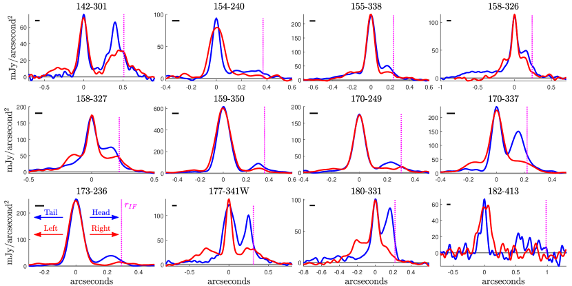
Figure 5: Surface brightness cuts across the Band 3 (r=0.5) images of the proplyds. Each cut is the mean value of a 9-pixel (0$\farcs$072) wide strip centered on the disk. Blue lines are head-to-tail cuts with the origin at the disk and positive values toward the head. Red lines are horizontal cuts when the proplyd is rotated with the head facing up. The vertical dotted magenta line shows the location of the outer edge of the ionization front ($r_{\text{IF}}$). The black line in the upper left indicates the minor axis of the beam (0$\farcs$057).

The 12 proplyds in our sample show a consistent pattern of morphology versus wavelength. At Band 7, only emission from the central disk is seen. At Band 3, both compact emission from the disk and extended emission from the ionization front are seen. Free-free emission from the proplyd tail is also seen in some sources, and it is more clear in the r=2.0 images. At centimeter wavelengths, the ionization front is clearly detected, but the disk is not seen (with the exception of 159-350). The pattern is due to the spectral dependence of thermal dust emission compared to free-free emission. The flux density of a dust disk decreases with increasing wavelength, following $F_{\nu}\propto\lambda^{-\alpha}$ with spectral index $\alpha$ = 1.5–3, making it difficult to detect at centimeter wavelengths. The spectral dependence of (optically thin) free-free emission is shallow, following $F_{\nu}\propto\lambda^{0.1}$, so its brightness dominates over dust at longer wavelengths. This behavior has been employed in previous studies to spectrally decompose dust from free-free emission for unresolved sources with no obvious propyld morphology (e.g., Mann et al., 2014; Sheehan et al., 2016; Eisner et al., 2018). With deep, high-resolution images of proplyds, as presented here, we can spatially isolate the dust disk from the surrounding free-free emission.

3.2 Additional Observed Features

HST images found arcs of emission beyond the ionization front of some proplyds (Bally et al., 1998a). These are bow shocks from the interaction of the outflowing material with the stellar wind of $\theta^{1}$ Ori C. We searched the region around these 12 proplyds in the Band 3 image for such arcs, and we located one around 180-331 (Figure 6). The arc is faint but detected as a coherent structure over the background noise, and it is coincident with the arc seen with HST.

The ALMA Band 3 image of 170-337 exhibits a “knot” of emission in the ionization front directly north of the disk. This marks the location where a jet from the disk breaks through the ionization front. The jet is known from prior HST observations (O’dell et al., 1997; Bally et al., 1998a, 2000). Faint emission is seen extending from the knot beyond the ionization front, likely tracing free-free emission from jet material that has been photoionized.

Two compact sources are observed near 177-341W in the ALMA Band 3 observations. One, east of the disk, was discovered in HST images by Bally et al. (1998a) and designated 177-341b. This source is not seen in Band 7 but is perhaps faintly visible in the VLA $K$ and $X$ band images. Bally et al. (2000) suggests this source may be a knot of emission caused by a jet or outflow from the disk in this proplyd. The second compact source is southeast of the disk near the end of the proplyd tail. This source shows opposite panchromatic behavior—it is clearly seen in ALMA Band 7 but not apparent at centimeter wavelengths, suggesting the emission is primarily from dust. 159-350 also has a companion source located northeast of the ionization front. It is seen in all wavelengths presented here, as well as in HST images (Bally et al., 1998a).

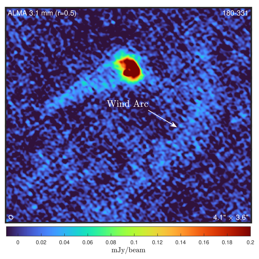
Figure 6: ALMA Band 3 image of the proplyd 180-331 showing the wind arc, which was also seen in HST images of this source. This is the only proplyd in our sample with a wind arc detected. The color scale is truncated, saturating the disk and proplyd head.

3.3 Disk Sizes

The ability of these observations to isolate the dust disks from the surrounding free-free emission allows us to study their sizes and masses, which are fundamental in determining the nature of the planetary system that can form.

We compute the disk radii as one-half of the FWHM of the deconvolved major axis, assuming a distance of 400 pc, and we report the results in Table 2. Disk radii range from 6.4 to 38 au, which are comparable to, or smaller than, the size of the solar system ($\sim$30 au), suggesting these disks will form compact planetary systems. The radii are consistent with typical dust disk sizes seen in the broader ONC population with ALMA (Eisner et al., 2018; Otter et al., 2021), providing further evidence that external photoevaporation—which is clearly impacting these proplyd systems—sets the disk sizes in the ONC more generally.

We compare the sizes of the proplyd disks measured at Band 3 and Band 7 (Figure 7). We find very good agreement for most of the disks ($\rho$ = 0.933 $\pm$ 0.036), although three are slightly smaller at Band 3. A smaller disk size at longer wavelengths is expected if larger grains (which emit more efficiently at longer wavelengths) are concentrated to smaller disk radii than smaller grains, as predicted by inward aerodynamic drift (Weidenschilling, 1977a). The absence of a size difference between wavelengths could indicate that drift is halted by, i.e., pressure bumps in the disk (Pinilla et al., 2012), that grains at all radii are sufficiently large to emit efficiently out to 3.1 mm, or that the disk is optically thick. High optical depth is likely for these systems (Section 3.4). Disks having similar sizes at Band 3 and Band 7 are not unique to the ONC; Tazzari et al. (2021a) found this to be the case for many disks in the Lupus star-forming region.

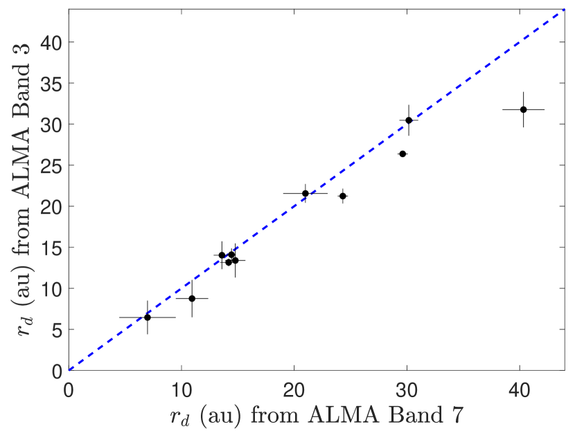
Figure 7: Size of the proplyd disks measured from ALMA Band 3 and Band 7 images. The sizes agree for most sources although three are slightly smaller at Band 3. Proplyd 182-413 was not covered by the Band 7 observations and thus is excluded from this plot.

We identify a correlation between $r_{d}$ and $d_{\perp}$ with $\rho$ = 0.741 $\pm$ 0.036 (Figure 8). This differs from the results of the larger ONC samples presented by Eisner et al. (2018) and Otter et al. (2021), who found no significant trend. Boyden & Eisner (2020) did, however, find a trend in gas disk radii with $d_{\perp}$. There is also a clear trend between $r_{d}$ and $r_{\textrm{IF}}$ with $\rho$ = 0.795 $\pm$ 0.041 (Figure 9), which was previously seen in HST images of proplyds (Vicente & Alves, 2005).

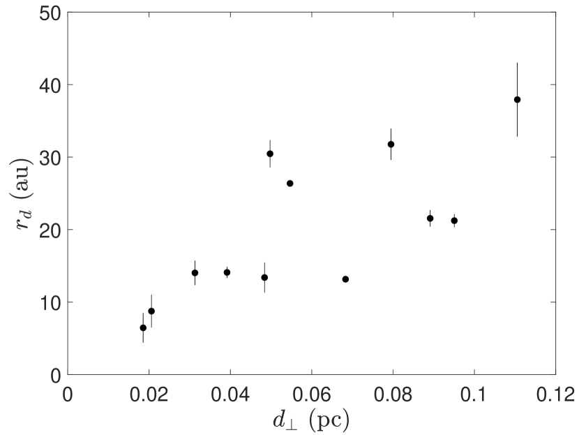
Figure 8: Size of the proplyd disks versus their projected separation from $\theta^{1}$ Ori C.

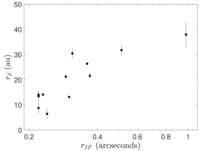
Figure 9: Size of the proplyd disks versus size of the proplyd ionization fronts.

In theory, external photoevaporation removes material from the disk beyond the “gravitational radius” ($r_{g}$). This the location where the sound speed of the gas ($c_{s}$) is equal to the escape speed from the star’s gravity, i.e., $r_{g}=GM_{\star}/c_{s}^{2}$. We compute $r_{g}$ for the eight systems with measured stellar masses (see Table 1) using $c_{s}$ = 3 km s^-1 as appropriate for an FUV-driven outflow (Johnstone et al., 1998; Winter & Haworth, 2022) and report the results in Table 2. We find $r_{d}/r_{g}$ ratios ranging from 1.33 to 0.19. The one system with $r_{d}$ $>$ $r_{g}$ (170-249) is undergoing photoevaporation in the “supercritical” regime (Adams et al., 2004) and may be at an earlier stage of the photoevaporation process. Systems with $r_{d}$ $<$ $r_{g}$ (but $r_{d}/r_{g}$ $\gtrsim$ 0.1–0.2) are consistent with results of detailed photoevaporation models in the “subcritical” regime (Adams et al., 2004). We note that our observations only probe the radii of the dust disks, which can be smaller than those of the gas disks if large grains have drifted inward. Gas disks larger than dust disks is regularly observed in both low-mass star-forming regions (Ansdell et al., 2018) and the ONC (Boyden & Eisner, 2020).

3.4 Disk Spectral Indices and Optical Depths

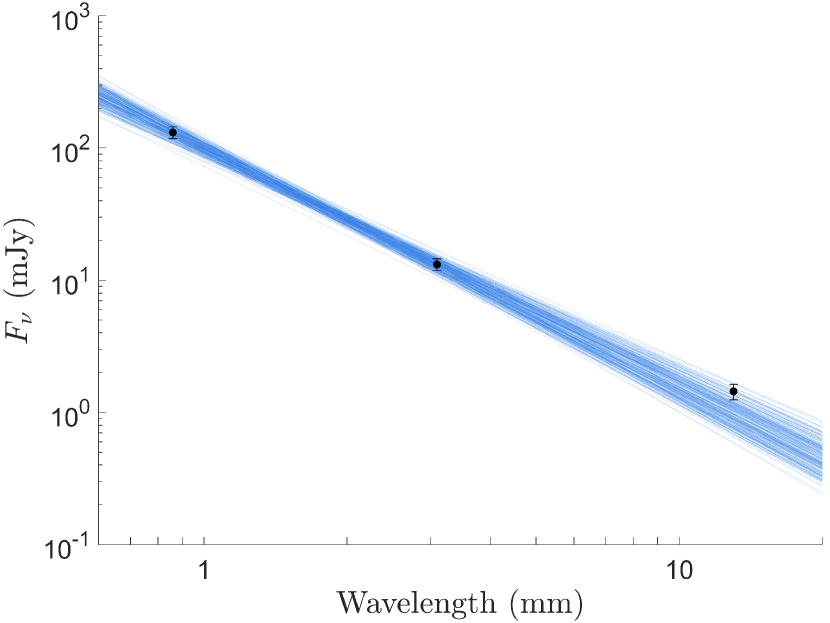
Figure 10: SED of the 159-350 disk, the only system in our sample with the disk component detected at VLA $K$ band. Black points are flux density measurements from ALMA Band 7, ALMA Band 3, and VLA $K$ Band. Error bars represent the total (measured plus calibration) uncertainty. Blue lines are 200 power-law fits to the two ALMA points while varying them within their uncertainties. The $K$ band flux density is consistent with these fits (and thus with arising from dust emission) although it is on the brighter end of the expected range.

The spectral dependence of disk flux density in the (sub)millimeter typically follows a power law $F_{\nu}\propto\lambda^{-\alpha}$. If the emission is optically thin and in the Rayleigh-Jeans regime, measuring the spectral index ($\alpha$) can reveal the index of the dust opacity spectrum ($\beta=\alpha-2$). The spectral index can thus inform us of the dust grain sizes, with shallower spectral indices indicating growth to larger grains. If the emission is optically thick, scattering can be significant, and the spectral index is shallower (closer to 2) and depends on the dust albedo (Liu, 2019; Zhu et al., 2019).

We measure the spectral indices of the disks from Band 7 to Band 3 for the eleven sources observed in both bands. Values are reported in Table 2. The uncertainties on $\alpha$ are propagated from statistical errors on the flux values returned from imfit plus a 10% error due to calibration uncertainty. We find $\alpha$ values from 1.6 to 2.1, strongly suggesting the emission is optically thick. If scattering is ignored, optically thick emission follows the Planck function, so $\alpha$ $<$ 2 requires cold dust in order to deviate from the Rayleigh-Jeans regime. For instance, the smallest spectral index in our sample, $\alpha$ = 1.61, would require a dust temperature of 14 K, which is colder than expected for disks in isolated environments, much less in the ONC. It is much more likely that $\alpha$ $<$ 2 is due to the scattering of radiation by dust with albedo that decreases with increasing wavelength (Liu, 2019; Zhu et al., 2019).

In principle, this behavior constrains the grain properties. Zhu et al. (2019) show that $\alpha$ $<$ 2 arises when the maximum grain size is around a few hundred microns. This is consistent with model predictions for dust at 10s of astronomical units in a 1 Myr old disk, as shown, for example, in Figure 5 of Rosotti et al. (2019). Models that include external photoevaporation, however, predict a reduction in the maximum grain size (Sellek et al., 2020). A detailed investigation into the grain properties of these disks could be carried out in a future paper.

Otter et al. (2021) found a large population of ONC sources with $\alpha\simeq 2$, consistent with our results. Tazzari et al. (2021b) measured $\alpha$ for disks in the Taurus, Lupus, and Ophiuchus low-mass star-forming regions, finding values from 1.7 to 2.9. The proplyd disk indices reported here fall into the lower end of this range. The high optical depth of ONC disks is likely a result of their small sizes. Tazzari et al. (2021a) found a trend of increasing $\alpha$ with disk size for systems in Lupus. We find no clear correlation between $\alpha$ and $r_{d}$ within our sample (Table 3), although the range of disk sizes over which to search for such a trend is limited. Studies of large and well-resolved disks have found $\alpha$ to be $<$ 2 in the inner (presumably more optically thick) regions (Tsukagoshi et al., 2016; Huang et al., 2018; Dent et al., 2019; Ribas et al., 2023). The proplyd disks may be similar, only with the outer parts removed by external photoevaporation.

For one source, 159-350, flux is clearly detected in the VLA $K$ Band (1.3 cm) at the location of the disk. The flux density is 1.44 $\pm$ 0.19 mJy, as found by imfit. We examine its spectral energy distribution (SED; Figure 10) to assess whether this emission arises from dust, free-free, or a nonthermal source of emission. Blue lines show a set of 200 power-law fits to the Band 7 and Band 3 flux densities, varied independently within their uncertainties. The $K$ band measurement is consistent with (although at the higher end of) these fits extrapolated to 1.3 cm. Thus, we conclude this emission comes primarily from dust, and that this disk likely remains optically thick to centimeter wavelengths. This disk is, by far, the brightest in our sample (4.5 times brighter than the second-brightest disk in ALMA Band 3), which explains why it is the only one detected with the VLA.

For some of the other disks, extrapolating the measured Band 3 fluxes to $K$ Band using the measured Band 7–3 spectral index predicts faint, but significant, detections. However, no clear disk components are observed. This suggests a steepening of the spectral index between 3.1 mm and 1.3 cm, likely due to the disks becoming optically thin or a change in the spectral dependence of the dust albedo. Future observations at wavelengths longer than 3.1 mm but sensitive enough to detect the dust disks would be useful to test this. Such measurements could come from deeper VLA observations, upcoming observations with ALMA Band 1, or future observations with the ngVLA.

3.5 Disk Masses and Temperatures

We compute the disk dust masses with the standard equation

$$M_{\text{d}}=\frac{F_{\nu}d^{2}}{\kappa B_{\nu}\left(T_{\text{d}}\right)}$$ (1)

(Hildebrand, 1983; Beckwith et al., 1990), where $F_{\nu}$ is the measured Band 3 flux density and $d$ is the distance from Earth (400 pc). $\kappa$ is the dust opacity, which we set to 1 cm² g^-1 based on the value of 2.3 cm² g^-1 used by Andrews et al. (2013) at 1.3 mm and the commonly assumed spectral dependence $\kappa\propto\lambda^{-1}$. $B_{\nu}\left(T_{\text{d}}\right)$ is the Planck function at the average dust temperature, for which we use two different choices. First, we use 20 K, which is the typically assumed dust temperature for disks in low-mass star-forming regions. Second, we use the temperature expected due to external heating by $\theta^{1}$ Ori C (Haworth, 2021). From balancing disk heating and cooling, this temperature is

$$T_{d}=T_{\star}\left(\frac{R_{\star}}{d_{\perp}}\right)^{1/2},$$ (2)

where $T_{\star}$ = 39,000 K and $R_{\star}$ = 10.6 $R_{\odot}$ are the temperature and radius of $\theta^{1}$ Ori C, respectively. We find $T_{d}$ $>$ 20 K in all cases, suggesting external heating dominates over internal heating when setting the disk temperatures. We report $T_{d}$ and both mass calculations in Table 2. The uncertainties we quote on the dust masses are simply the propagation of the uncertainty on the flux densities.

Assuming 20 K, disk dust masses range from 27 to 654 $M_{\oplus}$, with all but one of the disks having $M_{d}$ $>$ 33 $M_{\oplus}$, the mass of dust in models of the Minimum Mass Solar Nebula (Weidenschilling, 1977b). This suggests that these disks are capable of forming planetary systems like the solar system. With $T_{d}$ set by external heating, however, dust masses are lower (3.5–147 $M_{\oplus}$), and only two disks have $M_{d}$ $>$ 33 $M_{\oplus}$. We find no correlation between disk mass (actually disk flux) and $d_{\perp}$ (Table 3), in agreement with the findings by Otter et al. (2021) for a larger sample of ONC sources.

In Figure 11 we plot disk radii versus dust mass, and we see no significant trend between these properties. This is in contrast to low-mass star-forming regions where a trend does exist between disk size and mass (Tripathi et al., 2017; Andrews et al., 2018), which we show as a gray dotted line in Figure 11. We see that the proplyd disks are smaller than predicted by the trend established for disks in low-mass star-forming regions. No size–mass (or size–flux) trend was seen in prior ALMA studies of larger samples of ONC disks (Eisner et al., 2018; Otter et al., 2021). We also note that the proplyd disks are brighter than most other disks in the ONC, yielding a biased view of the size–mass parameter space relative to these prior studies.

Equation 1 assumes the dust emission is entirely optical thin. As discussed in Section 3.4, the measured spectral indices suggest high optical depth, leading the masses to be underestimated (Ballering & Eisner, 2019; Xin et al., 2023). The results are still useful as a lower limit on the dust masses and for comparison with masses of other disks calculated similarly. The effect on disk dust masses due to both temperature and optical depth effects can be accounted for with radiative transfer models (e.g., Ballering & Eisner, 2019), but such models are beyond the scope of this work.

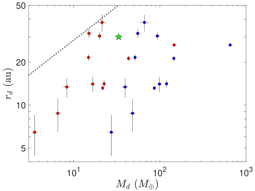
Figure 11: Disk radii and dust masses of the twelve proplyds in this sample. Masses computed assuming 20 K dust are in blue, whereas masses computed using a dust temperature set by external radiation ($T_{d}$) are in red. The green star is the Minimum Mass Solar Nebula. The gray dotted line is the disk size–mass relation found by Tripathi et al. (2017) in low-mass star-forming regions.

3.6 Mass-loss Rates

Measuring the photoevaporative mass-loss rate ($\dot{M}$) is critical to understanding the effect of the cluster environment on the planet-forming potential in disks. The FUV-driven wind from the disk surface is roughly symmetric (Winter & Haworth, 2022), so we compute the mass flow through a spherical surface at the location of the ionization front: $\dot{M}=4\pi r_{\text{IF}}^{2}\rho v$. This flow has a speed of 1–3 km s^-1, so we adopt $v$ = 2 km s^-1. The EUV radiation, primarily from the direction of $\theta^{1}$ Ori C, ionizes the near surface of the sphere (the proplyd head). This “lights up” a portion of the outflow, allowing us to probe the gas density of the outflow at the ionization front as $\rho=n_{e}\mu m_{H}$, where $n_{e}$ is the electron density and $\mu$ = 1.35 is the atomic weight of the gas per electron. Here we compute $n_{e}$ to evaluate $\dot{M}$ in two ways: first, by invoking ionization equilibrium ($\dot{M}_{\text{1}}$) and second, by using the measured brightness of the free-free emission from the ALMA observations ($\dot{M}_{\text{2}}$).

The condition of photoionization equilibrium requires that

$$\frac{\Phi}{4\pi d_{\perp}^{2}}=\frac{\alpha_{B}n_{e}^{2}r_{\text{IF}}}{3},$$ (3)

where $\alpha_{B}$ = 2.6 $\times$ $10^{-13}$ cm³ s^-1 is the recombination coefficient and $\Phi$ = 7.35 $\times$ 10⁴⁸ s^-1 is the flux of EUV photons from $\theta^{1}$ Ori C (O’Dell et al., 2017). Solving this for $n_{e}$ and combining with the mass-loss relation above yields

$$\dot{M}_{\text{1}}=\mu m_{H}v(12\pi\Phi/\alpha_{B})^{1/2}d_{\perp}^{-1}r_{\text{IF}}^{3/2}.$$ (4)

Values of $\dot{M}_{1}$ for these proplyds are reported in Table 2. The mass-loss rates range from 0.6 to 3.1 $\times$ 10^-7 $M_{\odot}$ yr^-1, which are generally consistent with mass-loss rates inferred from prior studies of ONC proplyds (e.g., Störzer & Hollenbach, 1999).

The second way we compute the mass-loss rate is by deriving $n_{e}$ from the brightness of the free-free emission. We do this via the “emission measure,” defined as $EM=n_{e}^{2}L$, where $L$ is the line-of-sight path length through the ionized gas. We first compute the optical depth of the observed free-free emission as $\tau_{\text{3.1mm}}=I_{\nu}/B_{\nu}(T_{e})$ (appropriate in the optically thin regime), where $I_{\nu}$ is the measured surface brightness of the ionization front in the Band 3 images and $B_{\nu}(T_{e})$ is the Planck Function for an electron temperature of $T_{e}$ = $10^{4}$ K. We find $\tau_{\text{3.1mm}}\sim 10^{-3}$ in the ionization fronts of these proplyds. We then compute the emission measure following Equation (A.1b) of Mezger & Henderson (1967):

$$\left(\frac{EM}{\text{pc}~{}\text{cm}^{-6}}\right)=\left(\frac{\tau_{\text{3.1mm}}}{3.28\times 10^{-7}}\right)\left(\frac{Te}{10^{4}\,K}\right)\left(\frac{\nu}{\text{GHz}}\right).$$ (5)

We find $EM\sim 10^{7}$–$10^{8}$ pc cm^-6 for these sources.

We model the ionization front as a thin hemispheric shell of radius $r_{\text{IF}}$ and thickness $\Delta r$. The maximum line-of-sight path length through such a shell is $L=2\sqrt{2r_{\text{IF}}\Delta r-\Delta r^{2}}\approx 2\sqrt{2r_{\text{IF}}\Delta r}$ when $\Delta r\ll r_{\text{IF}}$. The thickness of the ionization front is determined by the electron density as $\Delta r=(n_{e}\sigma)^{-1}$, where $\sigma=6.3\times 10^{-18}$ cm² is the ionization cross section. Thus, we can write the path length as $L=2\sqrt{2r_{\text{IF}}/n_{e}\sigma}$. Substituting this into the definition of the emission measure and solving for $n_{e}$, we find

$$n_{e}=\left(\frac{EM^{2}\sigma}{8r_{\text{IF}}}\right)^{1/3}.$$ (6)

Using Equation 6, we find $n_{e}$ of 0.7–3 $\times$ $10^{6}$ cm^-3, generally consistent with estimates of $n_{e}$ from other methods (Bally et al., 1998a). $n_{e}$ = $10^{6}$ cm^-3 results in $\Delta r$ = 0.01 au, so the ionization fronts are indeed quite thin.

Combining Equation 6 with the flow equation yields

$$\dot{M}_{\text{2}}=2\pi\mu m_{H}v\sigma^{1/3}EM^{2/3}r_{\text{IF}}^{5/3}.$$ (7)

We find $\dot{M}_{\text{2}}$ values of 3.2–18.4 $\times$ 10^-7 $M_{\odot}$ yr^-1, and we report the results in Table 2.

The $\dot{M}_{\text{2}}$ calculation yields larger estimates for the mass-loss rates than $\dot{M}_{\text{1}}$ by factors of 1.5–9.0. There are several uncertainties inherent in both calculations. $\Phi$ in Equation 4 only accounts for ionizing photons from $\theta^{1}$ Ori C, whereas other massive stars in the cluster likely contribute EUV flux as well. Accounting for these would yield a larger $\dot{M}_{\text{1}}$. On the other hand, Equation 4 does not account for attenuation between the ionizing sources and the proplyds, and $d_{\perp}$ is smaller than the true distance to the sources, both of which would lead to an overestimated $\dot{M}_{\text{1}}$. Regarding $\dot{M}_{\text{2}}$, our use of the thin shell model for the ionization front differs from that used in prior studies. Bally et al. (1998a), for example, used a more extended power-law profile. A thicker ionization front and correspondingly larger path length would yield lower values of $\dot{M}_{\text{2}}$ than we report. Overall, however, the decent agreement between two calculations that use different approaches gives confidence that these mass-loss rate estimates are accurate to within an order of magnitude or better.

Models by Johnstone et al. (1998) predict that if $\dot{M}$ is constant with $d_{\perp}$, we would observe $r_{\text{IF}}\propto d_{\perp}^{2/3}$. Figure 12 illustrates the relation between these variables. While they are positively correlated—as borne out by the Spearman correlation (Table 3)—they do not appear to follow a power-law relation. Indeed, as shown in the calculations above, $\dot{M}$ is not constant; it varies by a factor of $\sim$5 within this sample.

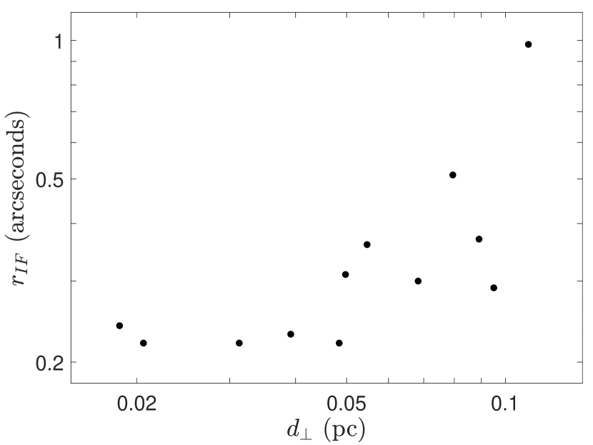
Figure 12: Size of the proplyd ionization fronts versus their projected separation from $\theta^{1}$ Ori C.

We compute the photoevaporative timescale by dividing the disk gas mass (dust mass $\times$ 100) by the mass-loss rate. Considering we have two estimates of the disk dust masses and two estimates of the mass-loss rates, we compute both a minimum, $t_{\text{min}}=100M_{d}(T_{d})/\dot{M}_{\text{2}}$, and maximum, $t_{\text{max}}=100M_{d}(20K)/\dot{M}_{\text{1}}$, estimate for the evaporative timescale. Values of $t_{\text{min}}$ range from 3.2 to 18.4 kyr and values of $t_{\text{max}}$ range from 37 to 1427 kyr; both are reported in Table 2. Most of the timescales are shorter than the age of these systems (1–2 Myr), implying that such systems should no longer host disks. This discrepancy is referred to as the “proplyd lifetime problem”.

Solutions to the proplyd lifetime problem suggested in the literature include: (1) disk masses are larger than typically measured due to being optically thick at (sub)millimeter wavelengths (Clarke, 2007); (2) low-mass stars in the ONC are on radial orbits and thus spend relatively little time in the high-UV environment (Störzer & Hollenbach, 1999); (3) multiple epochs of star formation occurred in the ONC, so some disks are younger than the median age (Beccari et al., 2017); (4) disks were shielded from the intense UV radiation by intervening gas in the cluster for a significant portion of their history (Qiao et al., 2022; Wilhelm et al., 2023); or some combination of the above (Winter et al., 2019). Our results offer no new insights on arguments (2), (3), or (4). However, we find that the disks are optically thick so the dust masses may be significantly underestimated, emphasizing the importance of argument (1).

In the timescale calculations, we assumed a gas-to-dust mass ratio of 100, as is found in the ISM. Whether this ratio holds for protoplanetary disks is a matter of debate and is closely tied to uncertainties in the disk abundance of CO (e.g., Schwarz et al., 2018; Zhang et al., 2019), the most readily observable gas tracer. The photoevaporation process preferentially removes gas and small grains, while the large grains, which we detect with ALMA, are not entrained in the outflow. Thus, photoevaporation could decrease the gas-to-dust ratio (Throop & Bally, 2005); although the large grains immune from evaporation are also the most susceptible to loss by inward drift in the absence of pressure traps (Sellek et al., 2020). By modeling ALMA CO and HCO⁺ observations of several ONC disks, Boyden & Eisner (2023) found gas-to-dust ratios $\geq$ 100, suggesting our use of the ISM value is justified.

4 Summary

We present ALMA Band 3 (3.1 mm) images of twelve ONC proplyds. With high sensitivity and angular resolution, these observations detect and isolate dust emission from the protoplanetary disk and free-free emission from the surrounding ionization front. A comparison with images at both shorter (ALMA Band 7) and longer (VLA) wavelengths further solidifies the morphology of these systems. Our main findings include:

• The disks are generally small, probably due to truncation by external photoevaporation. The sizes are consistent with the broader population of ONC disks measured in previous surveys. The resulting planetary systems will likely be more compact than the solar system. The disk sizes correlate with the size of the ionization front and with the distance from $\theta^{1}$ Ori C, but disk size and disk flux are not correlated.

• The spectral indices measured from Band 7 to Band 3 are shallow ($\alpha\lesssim 2.1$) suggesting the dust emission is optically thick. High optical depth is expected for massive but compact disks.

• According to the standard calculation of disk dust mass from millimeter flux, these disks are massive enough to form planetary systems like our solar system despite ongoing external photoevaporation. The high optical depth of the dust emission means the true masses could be significantly higher.

• The photoevaporative mass-loss rates, calculated by assuming photoionization equilibrium and from the brightness of the free-free emission, are generally consistent with prior HST-based estimates and suggest photoevaporation timescales shorter than the $\sim$1 Myr age of ONC—underscoring the “proplyd lifetime problem.” Disk masses that are underestimated due to being optically thick are a potential solution to this problem.

Future observations at longer wavelengths with comparable resolution and sufficient sensitivity to detect the dust emission will further reveal the properties of ONC proplyds. Such measurements could come from deeper VLA observations, upcoming observations with ALMA Band 1, or future observations with the ngVLA. At these longer wavelengths, the optical depth of the dust decreases, providing more reliable disk masses and better measurements of the grain properties from spectral indices. The free-free emission is also more prominent at longer wavelengths. This may expand the sample of well-resolved proplyds to systems with fainter ionization fronts. Our work demonstrates that even at wavelengths where free-free emission dominates over the dust, the two can be reliably isolated with high-resolution observations.

We thank the anonymous referee for many useful suggestions. We thank Andrew J. Winter for helpful discussions concerning the photoevaporative mass-loss rates. We thank NRAO staff, especially Brian Mason, for assistance with imaging the ALMA Band 3 data. We also gratefully acknowledge the use of NRAO computing facilities. This paper makes use of the following ALMA data: ADS/JAO.ALMA#2015.1.00534.S and ADS/JAO.ALMA#2018.1.01107.S. ALMA is a partnership of ESO (representing its member states), NSF (USA) and NINS (Japan), together with NRC (Canada), MOST and ASIAA (Taiwan), and KASI (Republic of Korea), in cooperation with the Republic of Chile. The Joint ALMA Observatory is operated by ESO, AUI/NRAO, and NAOJ. The National Radio Astronomy Observatory is a facility of the National Science Foundation operated under cooperative agreement by Associated Universities, Inc. N.P.B. acknowledges support from the Virginia Initiative on Cosmic Origins (VICO) and SOFIA Award 09-0181. L.I.C. acknowledges support from the David and Lucille Packard Foundation, Research Corporation for Science Advancement Cottrell Fellowship, NASA ATP 80NSSC20K0529, and NSF grant no. AST-2205698. T.J.H. acknowledges support from a Royal Society Dorothy Hodgkin Fellowship. A.G. acknowledges support from the NSF under AST 2008101 and CAREER 2142300. J.A.E and R.D.B acknowledge support by NSF AAG grant 1811290. J.A.E, J.S.K, and R.D.B acknowledge support by the National Aeronautics and Space Administration under Agreement No. 80NSSC21K0593 for the program “Alien Earths.” The results reported herein benefited from collaborations and/or information exchange within NASA’s Nexus for Exoplanet System Science (NExSS) research coordination network sponsored by NASA’s Science Mission Directorate.

References

- Adams (2010) Adams, F. C. 2010, ARA&A, 48, 47, doi: 10.1146/annurev-astro-081309-130830
- Adams et al. (2004) Adams, F. C., Hollenbach, D., Laughlin, G., & Gorti, U. 2004, ApJ, 611, 360, doi: 10.1086/421989
- Andrews et al. (2013) Andrews, S. M., Rosenfeld, K. A., Kraus, A. L., & Wilner, D. J. 2013, ApJ, 771, 129, doi: 10.1088/0004-637X/771/2/129
- Andrews et al. (2018) Andrews, S. M., Terrell, M., Tripathi, A., et al. 2018, ApJ, 865, 157, doi: 10.3847/1538-4357/aadd9f
- Ansdell et al. (2018) Ansdell, M., Williams, J. P., Trapman, L., et al. 2018, ApJ, 859, 21, doi: 10.3847/1538-4357/aab890
- Ballering & Eisner (2019) Ballering, N. P., & Eisner, J. A. 2019, AJ, 157, 144, doi: 10.3847/1538-3881/ab0a56
- Bally et al. (2000) Bally, J., O’Dell, C. R., & McCaughrean, M. J. 2000, AJ, 119, 2919, doi: 10.1086/301385
- Bally et al. (1998a) Bally, J., Sutherland, R. S., Devine, D., & Johnstone, D. 1998a, AJ, 116, 293, doi: 10.1086/300399
- Bally et al. (1998b) Bally, J., Testi, L., Sargent, A., & Carlstrom, J. 1998b, AJ, 116, 854, doi: 10.1086/300469
- Beccari et al. (2017) Beccari, G., Petr-Gotzens, M. G., Boffin, H. M. J., et al. 2017, A&A, 604, A22, doi: 10.1051/0004-6361/201730432
- Beckwith et al. (1990) Beckwith, S. V. W., Sargent, A. I., Chini, R. S., & Guesten, R. 1990, AJ, 99, 924, doi: 10.1086/115385
- Boyden & Eisner (2020) Boyden, R. D., & Eisner, J. A. 2020, ApJ, 894, 74, doi: 10.3847/1538-4357/ab86b7
- Boyden & Eisner (2023) —. 2023, ApJ, 947, 7, doi: 10.3847/1538-4357/acaf77
- Churchwell et al. (1987) Churchwell, E., Felli, M., Wood, D. O. S., & Massi, M. 1987, ApJ, 321, 516, doi: 10.1086/165648
- Clarke (2007) Clarke, C. J. 2007, MNRAS, 376, 1350, doi: 10.1111/j.1365-2966.2007.11547.x
- Dent et al. (2019) Dent, W. R. F., Pinte, C., Cortes, P. C., et al. 2019, MNRAS, 482, L29, doi: 10.1093/mnrasl/sly181
- Eisner et al. (2016) Eisner, J. A., Bally, J. M., Ginsburg, A., & Sheehan, P. D. 2016, ApJ, 826, 16, doi: 10.3847/0004-637X/826/1/16
- Eisner & Carpenter (2006) Eisner, J. A., & Carpenter, J. M. 2006, ApJ, 641, 1162, doi: 10.1086/500637
- Eisner et al. (2018) Eisner, J. A., Arce, H. G., Ballering, N. P., et al. 2018, ApJ, 860, 77, doi: 10.3847/1538-4357/aac3e2
- Fang et al. (2021) Fang, M., Kim, J. S., Pascucci, I., & Apai, D. 2021, ApJ, 908, 49, doi: 10.3847/1538-4357/abcec8
- Forbrich et al. (2016) Forbrich, J., Rivilla, V. M., Menten, K. M., et al. 2016, ApJ, 822, 93, doi: 10.3847/0004-637X/822/2/93
- Haworth (2021) Haworth, T. J. 2021, MNRAS, 503, 4172, doi: 10.1093/mnras/stab728
- Haworth et al. (2018) Haworth, T. J., Facchini, S., Clarke, C. J., & Mohanty, S. 2018, MNRAS, 475, 5460, doi: 10.1093/mnras/sty168
- Haworth et al. (2021) Haworth, T. J., Kim, J. S., Winter, A. J., et al. 2021, MNRAS, 501, 3502, doi: 10.1093/mnras/staa3918
- Hildebrand (1983) Hildebrand, R. H. 1983, QJRAS, 24, 267
- Huang et al. (2018) Huang, J., Andrews, S. M., Cleeves, L. I., et al. 2018, ApJ, 852, 122, doi: 10.3847/1538-4357/aaa1e7
- Jeffries (2007) Jeffries, R. D. 2007, MNRAS, 376, 1109, doi: 10.1111/j.1365-2966.2007.11471.x
- Johnstone et al. (1998) Johnstone, D., Hollenbach, D., & Bally, J. 1998, ApJ, 499, 758, doi: 10.1086/305658
- Kim et al. (2016) Kim, J. S., Clarke, C. J., Fang, M., & Facchini, S. 2016, ApJ, 826, L15, doi: 10.3847/2041-8205/826/1/L15
- Kounkel et al. (2017) Kounkel, M., Hartmann, L., Loinard, L., et al. 2017, ApJ, 834, 142, doi: 10.3847/1538-4357/834/2/142
- Kuffmeier et al. (2020) Kuffmeier, M., Zhao, B., & Caselli, P. 2020, A&A, 639, A86, doi: 10.1051/0004-6361/201937328
- Lada & Lada (2003) Lada, C. J., & Lada, E. A. 2003, ARA&A, 41, 57, doi: 10.1146/annurev.astro.41.011802.094844
- Liu (2019) Liu, H. B. 2019, ApJ, 877, L22, doi: 10.3847/2041-8213/ab1f8e
- Mann et al. (2014) Mann, R. K., Di Francesco, J., Johnstone, D., et al. 2014, ApJ, 784, 82, doi: 10.1088/0004-637X/784/1/82
- Marchington & Parker (2022) Marchington, B., & Parker, R. J. 2022, MNRAS, 515, 5449, doi: 10.1093/mnras/stac2145
- Menten et al. (2007) Menten, K. M., Reid, M. J., Forbrich, J., & Brunthaler, A. 2007, A&A, 474, 515, doi: 10.1051/0004-6361:20078247
- Mezger & Henderson (1967) Mezger, P. G., & Henderson, A. P. 1967, ApJ, 147, 471, doi: 10.1086/149030
- Mundy et al. (1995) Mundy, L. G., Looney, L. W., & Lada, E. A. 1995, ApJ, 452, L137, doi: 10.1086/309734
- O’dell et al. (1997) O’dell, C. R., Hartigan, P., Bally, J., & Morse, J. A. 1997, AJ, 114, 2016, doi: 10.1086/118622
- O’Dell et al. (2017) O’Dell, C. R., Kollatschny, W., & Ferland, G. J. 2017, ApJ, 837, 151, doi: 10.3847/1538-4357/aa6198
- O’dell & Wen (1994) O’dell, C. R., & Wen, Z. 1994, ApJ, 436, 194, doi: 10.1086/174892
- O’dell et al. (1993) O’dell, C. R., Wen, Z., & Hu, X. 1993, ApJ, 410, 696, doi: 10.1086/172786
- O’dell & Wong (1996) O’dell, C. R., & Wong, K. 1996, AJ, 111, 846, doi: 10.1086/117832
- Otter et al. (2021) Otter, J., Ginsburg, A., Ballering, N. P., et al. 2021, ApJ, 923, 221, doi: 10.3847/1538-4357/ac29c2
- Pinilla et al. (2012) Pinilla, P., Birnstiel, T., Ricci, L., et al. 2012, A&A, 538, A114, doi: 10.1051/0004-6361/201118204
- Qiao et al. (2023) Qiao, L., Coleman, G. A. L., & Haworth, T. J. 2023, MNRAS, 522, 1939, doi: 10.1093/mnras/stad944
- Qiao et al. (2022) Qiao, L., Haworth, T. J., Sellek, A. D., & Ali, A. A. 2022, MNRAS, 512, 3788, doi: 10.1093/mnras/stac684
- Ribas et al. (2023) Ribas, Á., Macías, E., Weber, P., et al. 2023, A&A, 673, A77, doi: 10.1051/0004-6361/202245637
- Ricci et al. (2008) Ricci, L., Robberto, M., & Soderblom, D. R. 2008, AJ, 136, 2136, doi: 10.1088/0004-6256/136/5/2136
- Robberto et al. (2013) Robberto, M., Soderblom, D. R., Bergeron, E., et al. 2013, ApJS, 207, 10, doi: 10.1088/0067-0049/207/1/10
- Rosotti et al. (2019) Rosotti, G. P., Tazzari, M., Booth, R. A., et al. 2019, MNRAS, 486, 4829, doi: 10.1093/mnras/stz1190
- Schwarz et al. (2018) Schwarz, K. R., Bergin, E. A., Cleeves, L. I., et al. 2018, ApJ, 856, 85, doi: 10.3847/1538-4357/aaae08
- Sellek et al. (2020) Sellek, A. D., Booth, R. A., & Clarke, C. J. 2020, MNRAS, 492, 1279, doi: 10.1093/mnras/stz3528
- Sheehan et al. (2016) Sheehan, P. D., Eisner, J. A., Mann, R. K., & Williams, J. P. 2016, ApJ, 831, 155, doi: 10.3847/0004-637X/831/2/155
- Sota et al. (2011) Sota, A., Maíz Apellániz, J., Walborn, N. R., et al. 2011, ApJS, 193, 24, doi: 10.1088/0067-0049/193/2/24
- Störzer & Hollenbach (1999) Störzer, H., & Hollenbach, D. 1999, ApJ, 515, 669, doi: 10.1086/307055
- Tazzari et al. (2021a) Tazzari, M., Clarke, C. J., Testi, L., et al. 2021a, MNRAS, 506, 2804, doi: 10.1093/mnras/stab1808
- Tazzari et al. (2021b) Tazzari, M., Testi, L., Natta, A., et al. 2021b, MNRAS, 506, 5117, doi: 10.1093/mnras/stab1912
- Throop & Bally (2005) Throop, H. B., & Bally, J. 2005, ApJ, 623, L149, doi: 10.1086/430272
- Tripathi et al. (2017) Tripathi, A., Andrews, S. M., Birnstiel, T., & Wilner, D. J. 2017, ApJ, 845, 44, doi: 10.3847/1538-4357/aa7c62
- Tsukagoshi et al. (2016) Tsukagoshi, T., Nomura, H., Muto, T., et al. 2016, ApJ, 829, L35, doi: 10.3847/2041-8205/829/2/L35
- Vicente & Alves (2005) Vicente, S. M., & Alves, J. 2005, A&A, 441, 195, doi: 10.1051/0004-6361:20053540
- Walsh et al. (2013) Walsh, C., Millar, T. J., & Nomura, H. 2013, ApJ, 766, L23, doi: 10.1088/2041-8205/766/2/L23
- Weidenschilling (1977a) Weidenschilling, S. J. 1977a, MNRAS, 180, 57, doi: 10.1093/mnras/180.2.57
- Weidenschilling (1977b) —. 1977b, Ap&SS, 51, 153, doi: 10.1007/BF00642464
- Wijnen et al. (2017) Wijnen, T. P. G., Pols, O. R., Pelupessy, F. I., & Portegies Zwart, S. 2017, A&A, 604, A91, doi: 10.1051/0004-6361/201731072
- Wilhelm et al. (2023) Wilhelm, M. J. C., Portegies Zwart, S., Cournoyer-Cloutier, C., et al. 2023, MNRAS, 520, 5331, doi: 10.1093/mnras/stad445
- Williams et al. (2005) Williams, J. P., Andrews, S. M., & Wilner, D. J. 2005, ApJ, 634, 495, doi: 10.1086/444493
- Winter et al. (2018) Winter, A. J., Clarke, C. J., Rosotti, G., et al. 2018, MNRAS, 478, 2700, doi: 10.1093/mnras/sty984
- Winter et al. (2019) Winter, A. J., Clarke, C. J., Rosotti, G. P., Hacar, A., & Alexander, R. 2019, MNRAS, 490, 5478, doi: 10.1093/mnras/stz2545
- Winter & Haworth (2022) Winter, A. J., & Haworth, T. J. 2022, European Physical Journal Plus, 137, 1132, doi: 10.1140/epjp/s13360-022-03314-1
- Winter et al. (2022) Winter, A. J., Haworth, T. J., Coleman, G. A. L., & Nayakshin, S. 2022, MNRAS, 515, 4287, doi: 10.1093/mnras/stac1564
- Xin et al. (2023) Xin, Z., Espaillat, C. C., Rilinger, A. M., Ribas, Á., & Macías, E. 2023, ApJ, 942, 4, doi: 10.3847/1538-4357/aca52b
- Zhang et al. (2019) Zhang, K., Bergin, E. A., Schwarz, K., Krijt, S., & Ciesla, F. 2019, ApJ, 883, 98, doi: 10.3847/1538-4357/ab38b9
- Zhu et al. (2019) Zhu, Z., Zhang, S., Jiang, Y.-F., et al. 2019, ApJ, 877, L18, doi: 10.3847/2041-8213/ab1f8c