Close Encounter of Three Black Holes Revisited

Abstract

We study the evolution of close triple black hole system with full numerical relativity techniques. We consider an equal mass non spinning hierarchical system with an inner binary ten orbits away from merger and study the effects of the third outer black hole on the binary’s merger time and its eccentricity evolution. We find a generic time delay and an increase in the number of orbits to merger of the binary, that can be modeled versus the distance $D$ to the third black hole as $\sim 1/D^{2.5}$. On the other hand, we find that the orientation of the third black hole orbit has little effect on the binary’s merger time when considering a fiducial initial distance of $D=30M$ to the binary (with initial orbital separation $d=8M$). In those scenarios the evolution of the inner binary eccentricity presents a steady decay, roughly as expected, but in addition shows a modulation with the time scale of the outer third black hole orbital semiperiod around the binary, resembling a beating frequency.

I Introduction

Triple black hole systems have a renewed interest since the observation that some of the gravitational waves signals detected by the LIGO-Virgo collaboration may be the product of highly eccentric black hole mergers Gayathri et al. (2022) and that one of the scenarios for creating those eccentricities may be the product of three body Lidov-Kozai interactions Yu et al. (2020). In this scenario, a tertiary companion on a sufficiently inclined outer orbit could drive the inner binary to extreme eccentricities, leading to efficient gravitational radiation and orbital decay. Also see Dall’Amico et al. (2021) for a formation scenario of GW190521 via three-body encounters in young massive star clusters.

The triple channel predicts a distinct region of the total mass, mass ratio, and spin parameter space for merging binary black holes, which can be used to disentangle the triple contribution to the overall observed gravitational wave sources. For a detailed study of the mass ratio distribution of binary black hole mergers induced by tertiary companions in triple systems see Ref. Martinez et al. (2022). Close encounters of stars with stellar-mass black hole binaries have been studied in Ryu et al. (2022).

Close encounters of three black holes require Numerical Relativity techniques. Full numerical evolution of triple systems are challenging due to the need to track three black holes and the different scales of time-integration involved in the solution. In Ref. Campanelli et al. (2008); Lousto and Zlochower (2008) we have performed prototypical evolutions of such systems and evaluated its accuracy compared to Newtonian and post-Newtonian evolutions Lousto and Nakano (2008).

In this paper we will revisit this scenario and evolve triple systems using full numerical techniques to assess the prompt or delayed merger and eccentricity evolution of a binary in a hierarchical triple system.

II Approximate initial data

In Ref. Lousto and Zlochower (2008) we have performed the three black holes prototypical studies from approximate initial data, based on Laguna (2004) and extended to include terms of the sort $\vec{S}_{i}\times\vec{P}_{i}$ representing interactions of spin with linear momentum in an expansion to leading order on those intrinsic parameters of the holes. In Galaviz et al. (2010) a similar study was made using exact initial data and found (when using the same raw 3BH parameters) some deviations in the long term evolutions when compared to the corresponding approximate initial data. Here we will introduce two sets improvements to the approximate initial data for multi black hole configurations. As already pointed out in Lousto and Zlochower (2008), a normalization for the parameters makes notable improvements in, for instance, the resulting waveforms of 2BH (See Fig. 1 in Lousto and Zlochower (2008)). To that end we will normalize data to the initial (sum of) horizon masses as computed fully numerically. The second improvement is to compute the next order expansion in the solutions to the Bowen-York Bowen and York (1980) initial data set. We will test those improvements by direct comparison with the “exact” initial data for 2BH.

Here we provide some details on how we find a perturbative solution of the Hamiltonian constraint equation, since in the Bowen-York approach Bowen and York (1980) the momentum constraint is solved exactly. Hence, the scope of this section is to solve perturbatively the partial differential equation for the conformal factor $\phi$

$$\Delta\phi=-\frac{1}{8}\phi^{-7}\hat{A}^{ij}\hat{A}_{ij},$$ (1)

with

$$\hat{A}^{ij}=\sum_{a}^{N_{BHs}}\left(\frac{3}{2r_{a}^{2}}\left[2P_{a}^{(i}n_{a}^{j)}+(n_{a}^{i}n_{a}^{j}-\eta^{ij})P_{ak}n_{a}^{k}\right]\right.$$

$$\left.+\frac{6}{r_{a}^{3}}n_{a}^{(i}\epsilon^{j)kl}J_{ak}n_{al}\right),$$ (2)

where we label the momentum and the spin of the holes as $\textbf{P}_{i}$ and $\textbf{J}_{i}$, following the notation of Lousto and Zlochower (2008).

For this purpose we start from the analytical solution at order 0th given by

$$\phi_{0}=1+\sum_{a}^{N_{BHs}}\frac{m_{a}}{2r_{a}},$$ (3)

which solves

$$\Delta\phi_{0}=0.$$ (4)

To find the first perturbative order $u$ of the solution we consider the equation

$$\Delta u_{1}=-\frac{1}{8}\phi_{0}^{-7}\hat{A}^{ij}\hat{A}_{ij}.$$ (5)

II.1 One Black Hole

Let us consider Eq. (5) for a single black hole. The term $\hat{A}^{ij}\hat{A}_{ij}$ is given by

$$\hat{A}^{ij}\hat{A}_{ij}=\frac{18J^{2}}{r^{6}}\left(1-x_{\textbf{J}}^{2}\right)+\frac{9P^{2}}{2r^{4}}\left(2x_{\textbf{P}}^{2}-1\right)+\frac{18}{r^{5}}x_{\textbf{P}\times\textbf{J}}\lVert\textbf{P}\times\textbf{J}\rVert,$$ (6)

where $x_{\textbf{J}}$, $x_{\textbf{P}}$ and $x_{\textbf{P}\times\textbf{J}}$ are respectively $\cos{\theta_{\textbf{J}}}$, $\cos{\theta_{\textbf{P}}}$ and $\cos{\theta_{\textbf{P}\times\textbf{J}}}$.

Since Eq. (5) is linear, the solution can be written as

$$u_{1}=F(r,x_{\textbf{P}})\textbf{P}^{2}+G(r,x_{\textbf{J}})\textbf{J}^{2}+H(r,x_{\textbf{P}\times\textbf{J}})\lVert\textbf{J}\times\textbf{P}\rVert.$$ (7)

In this way we can solve the equation separately for the functions $F(r,x_{\textbf{P}})$, $G(r,x_{\textbf{J}})$, $H(r,x_{\textbf{P}\times\textbf{J}})$.

In particular, it is convenient to write the source term in terms of Legendre polynomials. By doing so, we can solve the angular part of the equations algebraically

$$\begin{split}&\Delta F(r,x_{\textbf{P}})=\frac{3}{2r^{4}}\left(5P_{0}(x_{\textbf{P}})+4P_{2}(x_{\textbf{P}})\right),\\ &\Delta G(r,x_{\textbf{J}})=\frac{12J^{2}}{r^{6}}\left(P_{0}(x_{\textbf{J}})-P_{2}(x_{\textbf{J}})\right),\\ &\Delta H(r,x_{\textbf{P}\times\textbf{J}})=\frac{18}{r^{5}}P_{1}(x_{\textbf{P}\times\textbf{J}}).\end{split}$$ (8)

Thus the solution to first order is

$$\phi_{1}=\phi_{0}+F(r,x_{\textbf{P}})\textbf{P}^{2}+G(r,x_{\textbf{J}})\textbf{J}^{2}+H(r,x_{\textbf{P}\times\textbf{J}})\lVert\textbf{J}\times\textbf{P}\rVert,$$ (9)

where the functions $F(r,x_{\textbf{P}})$, $G(r,x_{\textbf{J}})$, $H(r,x_{\textbf{P}\times\textbf{J}})$ are explicitly given by

$$\begin{split}&F(r,x_{\textbf{P}})=\frac{1}{160(u+1)^{5}}[u^{4}(3x_{\textbf{P}}^{2}-1)(84u^{5}+378u^{4}\\ &\quad\quad+658u^{3}+539u^{2}+192u+84(u+1)^{5}u\log(u)\\ &\quad\quad-84(u+1)^{5}u\log(u+1)+15)]+\frac{u^{2}}{32}\left(1-\frac{1}{(u+1)^{5}}\right),\\ &G(r,x_{\textbf{J}})=\frac{u^{5}\left(1-3x_{\textbf{J}}^{2}\right)}{40(u+1)^{5}}+\frac{\left(u^{4}+5u^{3}+10u^{2}+5u+1\right)u^{3}}{40(u+1)^{5}},\\ &H(r,x_{\textbf{P}\times\textbf{J}})=-\frac{u^{4}\left(u^{2}+5u+10\right)x_{\textbf{P}\times\textbf{J}}}{80(u+1)^{5}},\end{split}$$ (10)

where $u=\frac{m}{2r}$ and this solution agrees with the one given in Lousto and Zlochower (2008).

Thus when we want to solve the second order perturbation equation for a single BH we have

$$\Delta\phi_{2}=-\frac{1}{8}\phi_{0}^{-7}\left(1-7u_{1}\right)\hat{A}^{ij}\hat{A}_{ij},$$ (11)

where we used the fact that $\phi_{1}^{-7}\approx\phi_{0}^{-7}(1-7u_{1})$ and hence

$$\Delta u_{2}=\frac{7}{8}\phi_{0}^{-7}u_{1}\hat{A}^{ij}\hat{A}_{ij}.$$ (12)

Using the same expansion reasoning we used for the 1st order case we can write

$$\begin{split}u_{2}=&F_{P^{4}}(r,x_{\textbf{P}})P^{4}+F_{J^{4}}(r,x_{\textbf{J}})J^{4}\\ &+F_{({\textbf{P}\times\textbf{J}})^{2}}(r,x_{\textbf{P}\times\textbf{J}})\lVert{\textbf{P}\times\textbf{J}}\rVert^{2}\\ &+F_{P({\textbf{P}\times\textbf{J}})}(r,x_{\textbf{P}},\phi_{\textbf{P}})P\lVert{\textbf{P}\times\textbf{J}}\rVert\\ &+F_{J({\textbf{P}\times\textbf{J}})}(r,x_{\textbf{J}},\phi_{\textbf{J}})J\lVert{\textbf{P}\times\textbf{J}}\rVert\\ &+F_{J^{2}P^{2}}(r,x_{\textbf{P}},\phi_{\textbf{P}})J^{2}P^{2}.\\ \end{split}$$ (13)

Note that in Eq.(13) there are terms that involve combinations of the vectors P, J, $\textbf{P}\times\textbf{J}$. For example, when solving for the term $F_{J({\textbf{P}\times\textbf{J}})}(r,x_{\textbf{J}},\phi_{\textbf{J}})$ we need to write $x_{\textbf{P}\times\textbf{J}}$ in terms of $x_{\textbf{J}}$ and $\phi_{\textbf{J}}$, as described in Appendix A. At this point, we can solve for the single functions in Eq.(13) as we did for Eq.(5) with the only difference that we need a decomposition in spherical harmonics and then solve the resulting ordinary differential equation in the variable $r$.

II.2 Two Black Holes

When we want to consider two BHs we proceed in the following way. First, let us assume that our system is bound so that we can then assume the Virial theorem to hold approximately true, $P^{2}\approx\frac{1}{r_{12}}$ where $r_{12}$ is the distance between the two BHs. Then we treat the solution as a superposition of the solutions for single black holes, where we also add a term due to the interaction between the two. Under this assumptions let us solve Eq.(5) for two BHs considering the perturbation of the second black hole on the first one. In this case we have

$$\frac{1}{r_{2}}=\frac{1}{r_{12}}+\mathcal{O}\left(\frac{1}{r_{12}}\right)^{2},$$ (14)

Hence we get

$$\begin{split}\hat{A}_{ij}\hat{A}^{ij}&=\frac{18J_{1}^{2}}{r_{1}^{6}}\left(1-x_{\textbf{J}_{1}}^{2}\right)+\frac{9P_{1}^{2}}{2r_{1}^{4}}\left(2x_{\textbf{P}_{1}}^{2}-1\right)\\ &+\frac{18}{r_{1}^{5}}x_{\textbf{P}_{1}\times\textbf{J}_{1}}\textbf{P}_{1}\times\textbf{J}_{1}+\mathcal{O}\left(\frac{1}{r_{12}}\right)^{2}\end{split}$$ (15)

and

$$\phi_{0}=1+\frac{m_{1}}{2r_{1}}+\frac{m_{2}}{2r_{2}}=1+\frac{m_{1}}{2r_{1}}+\frac{m_{2}}{2r_{12}}+\mathcal{O}\left(\frac{1}{r_{12}}\right)^{2},$$ (16)

Thus we can write

$$\begin{split}\phi_{0}^{-7}\hat{A}_{ij}\hat{A}^{ij}&=\left(1+\frac{m_{1}}{2r_{1}}\right)^{-7}\left(\frac{18J_{1}^{2}}{r_{1}^{6}}\left(1-x_{\textbf{J}_{1}}^{2}\right)\right.\\ &\left.+\frac{9P_{1}^{2}}{2r_{1}^{4}}\left(2x_{\textbf{P}_{1}}^{2}-1\right)+\frac{18}{r_{1}^{5}}x_{\textbf{P}_{1}\times\textbf{J}_{1}}\textbf{P}_{1}\times\textbf{J}_{1}\right)\\ &+\mathcal{O}\left(\frac{P^{2}}{r_{12}}\right)+\mathcal{O}\left(\frac{J^{2}}{r_{12}}\right)+\mathcal{O}\left(\frac{\textbf{P}\times\textbf{J}}{r_{12}}\right).\end{split}$$ (17)

As a result we can see that to first order the solution of Eq. (5) for two BHs is the superposition of the solutions for single black holes.

To second order we have

$$\begin{split}\phi_{1}^{-7}\hat{A}_{ij}\hat{A}^{ij}=&\left(1+\frac{m_{1}}{2r_{1}}+\frac{m_{2}}{2r_{2}}+u_{1}^{1}+u_{1}^{2}\right)^{-7}\\ &\left[\hat{A_{1}}_{ij}\hat{A_{1}}^{ij}+\hat{A_{2}}_{ij}\hat{A_{2}}^{ij}+2\hat{A_{1}}_{ij}\hat{A_{2}}^{ij}\right]\\ =&\left(1+\frac{m_{1}}{2r_{1}}\right)^{-7}\hat{A_{1}}_{ij}\hat{A_{1}}^{ij}-7\phi_{01}^{-7}u_{1}^{1}\hat{A_{1}}_{ij}\hat{A_{1}}^{ij}\\ &-7\phi_{01}^{-7}\frac{m_{2}}{2r_{12}}\hat{A_{1}}_{ij}\hat{A_{1}}^{ij}\\ &+\mathcal{O}\left(\frac{P^{4}}{r_{12}}\right)+\mathcal{O}\left(\frac{J^{4}}{r_{12}}\right)+\mathcal{O}\left(\frac{J^{2}P^{2}}{r_{12}}\right)\\ &+\mathcal{O}\left(J^{6}\right)+\mathcal{O}\left(P^{6}\right)+\mathcal{O}\left(P^{5}J\right)+\mathcal{O}\left(J^{5}P\right)\\ &+\mathcal{O}\left(J^{4}P^{2}\right)+\mathcal{O}\left(J^{3}P^{3}\right)+\mathcal{O}\left(J^{2}P^{4}\right).\end{split}$$ (18)

In this case we considered the second black hole as a perturbation of the first one, but the opposite is also true, so that the complete source term at second order is given by

$$\begin{split}\phi_{1}^{-7}\hat{A}_{ij}\hat{A}^{ij}=&\left(1+\frac{m_{1}}{2r_{1}}+\frac{m_{2}}{2r_{2}}+u_{1}^{1}+u_{1}^{2}\right)^{-7}\\ &\left[\hat{A_{1}}_{ij}\hat{A_{1}}^{ij}+\hat{A_{2}}_{ij}\hat{A_{2}}^{ij}+2\hat{A_{1}}_{ij}\hat{A_{2}}^{ij}\right]\\ =&\left(1+\frac{m_{1}}{2r_{1}}\right)^{-7}\hat{A_{1}}_{ij}\hat{A_{1}}^{ij}-7\phi_{01}^{-7}u_{1}^{1}\hat{A_{1}}_{ij}\hat{A_{1}}^{ij}\\ &-7\phi_{01}^{-7}\frac{m_{2}}{2r_{12}}\hat{A_{1}}_{ij}\hat{A_{1}}^{ij}\\ &+\left(1+\frac{m_{2}}{2r_{2}}\right)^{-7}\hat{A_{2}}_{ij}\hat{A_{2}}^{ij}-7\phi_{02}^{-7}u_{1}^{2}\hat{A_{2}}_{ij}\hat{A_{2}}^{ij}\\ &-7\phi_{02}^{-7}\frac{m_{1}}{2r_{12}}\hat{A_{2}}_{ij}\hat{A_{2}}^{ij}\\ &+\mathcal{O}\left(\frac{P^{4}}{r_{12}}\right)+\mathcal{O}\left(\frac{J^{4}}{r_{12}}\right)+\mathcal{O}\left(\frac{J^{2}P^{2}}{r_{12}}\right)\\ &+\mathcal{O}\left(J^{6}\right)+\mathcal{O}\left(P^{6}\right)+\mathcal{O}\left(P^{5}J\right)+\mathcal{O}\left(J^{5}P\right)\\ &+\mathcal{O}\left(J^{4}P^{2}\right)+\mathcal{O}\left(J^{3}P^{3}\right)+\mathcal{O}\left(J^{2}P^{4}\right).\end{split}$$ (19)

Eq.(19) implies that at second order we have to solve the partial differential equation

$$\begin{split}\Delta u_{2}=&+\frac{7}{8}\phi_{01}^{-7}u_{1}^{1}\hat{A_{1}}_{ij}\hat{A_{1}}^{ij}+\frac{7}{8}\phi_{01}^{-7}\frac{m_{2}}{2r_{12}}\hat{A_{1}}_{ij}\hat{A_{1}}^{ij}\\ &+\frac{7}{8}\phi_{02}^{-7}u_{1}^{2}\hat{A_{2}}_{ij}\hat{A_{2}}^{ij}+\frac{7}{8}\phi_{02}^{-7}\frac{m_{1}}{2r_{12}}\hat{A_{2}}_{ij}\hat{A_{2}}^{ij}.\end{split}$$ (20)

Then if we write $u_{2}=u_{2}^{1}+u_{2}^{2}$ we can solve independently for the two BHs

$$\begin{split}\Delta u_{2}^{1}=&+\frac{7}{8}\phi_{01}^{-7}u_{1}^{1}\hat{A_{1}}_{ij}\hat{A_{1}}^{ij}+\frac{7}{8}\phi_{01}^{-7}\frac{m_{2}}{2r_{12}}\hat{A_{1}}_{ij}\hat{A_{1}}^{ij}\\ \Delta u_{2}^{2}=&+\frac{7}{8}\phi_{02}^{-7}u_{1}^{2}\hat{A_{2}}_{ij}\hat{A_{2}}^{ij}+\frac{7}{8}\phi_{02}^{-7}\frac{m_{1}}{2r_{12}}\hat{A_{2}}_{ij}\hat{A_{2}}^{ij}.\end{split}$$ (21)

And again, by performing a decomposition in spherical harmonics we can reduce this system of partial differential equations to a set of independent ordinary differential equations. We also point out that this method can be straightforwardly generalized to an arbitrary number of BHs as follows

$$\Delta u_{2}^{\alpha}=+\frac{7}{8}\phi_{0\alpha}^{-7}u_{1}^{\alpha}\hat{A_{\alpha}}_{ij}\hat{A_{\alpha}}^{ij}+\sum_{\beta\neq\alpha}^{N_{BHs}}\frac{7}{8}\phi_{0\alpha}^{-7}\frac{m_{\beta}}{2r_{\alpha\beta}}\hat{A_{\alpha}}_{ij}\hat{A_{\alpha}}^{ij}.$$ (22)

with $\alpha=1,2,3,...,N_{BHs}$.

The total ADM mass at the second perturbative order is

$$\begin{split}M_{ADM}&=\sum_{i}^{N_{BHs}}\sum_{j\neq i}^{N_{BHs}}\\ &\frac{P_{i}^{2}}{2640000m_{i}^{5}}\Big{[}(160J_{i}^{2}(1448{R_{PJ}^{31}}^{2}+1448{R_{PJ}^{32}}^{2}\\ &+1529{R_{PJ}^{33}}^{2}-8000)\\ &+\frac{1650000m_{i}^{4}(s_{ij}-3m_{j})}{s_{ij}}-520157m_{i}^{2}P_{i}^{2})\Big{]}\\ &-\frac{266J_{i}^{4}}{825M_{i}^{7}}-\frac{2J_{i}^{2}(2m_{j}-s_{ij})}{5m_{i}^{3}s_{ij}}-\frac{3\lVert\textbf{P}_{i}\times\textbf{J}_{i}\rVert}{110m_{i}^{5}}+m_{i}\end{split}$$ (23)

where $R_{PJ}$ is the rotation matrix from the system with $\hat{P}=(0,0,1)$ to the system with $\hat{J}=(0,0,1)$ defined in Appendix A.

The total ADM linear momentum and angular momentum of the Bowen-York data are given by:

$$\vec{P}_{\rm ADM} = \sum_{i}^{N_{BHs}}\vec{P}_{i},$$ (24)

$$\vec{J}_{\rm ADM} = \sum_{i}^{N_{BHs}}(\vec{J}_{i}+\vec{r}_{i}\times\vec{P}_{i}).$$ (25)

III Full Numerical Techniques

In order to perform the full numerical simulations we use the LazEv codeZlochower et al. (2005) with 8th order spatial finite differences Lousto and Zlochower (2008), 4th order Runge-Kutta time integration with a Courant factor $(dt/dx=1/4)$.

To compute the numerical initial data, we use the puncture approach Brandt and Brügmann (1997) along with the TwoPunctures  Ansorg et al. (2004) code. We use AHFinderDirect Thornburg (2004) to locate apparent horizons. We measure the magnitude of the horizon spin $S_{H}$, using the isolated horizon algorithm as implemented in Ref. Campanelli et al. (2007). We can then calculate the horizon mass via the Christodoulou formula ${m^{H}}=\sqrt{m_{\rm irr}^{2}+S_{H}^{2}/(4m_{\rm irr}^{2})}\,,$ where $m_{\rm irr}=\sqrt{A_{H}/(16\pi)}$ and $A_{H}$ is the surface area of the horizon.

The Carpet Schnetter et al. (2004) mesh refinement driver provides a “moving boxes” style of mesh refinement. In this approach, refined grids of fixed size are arranged about the coordinate centers of the holes. The code then moves these fine grids about the computational domain by following the trajectories of the black holes.

The grid structure of our mesh refinements have a size of the largest box for all simulations of $\pm 400M$. The number of points between 0 and 400 on the coarsest grid is XXX in nXXX (i.e. n100 has 100 points). So, the grid spacing on the coarsest level is 400/XXX. The resolution in the wavezone is $100M/$XXX (i.e. n100 has $M/1.00$, n120 has $M/1.2$ and n144 has $M/1.44$) and the rest of the levels is adjusted globally. For instance, the grid around one of the black holes ($m_{1}$) is fixed at $\pm 0.6M$ in size and is the 9th refinement level. Therefore the grid spacing is 400/XXX/$2^{8}$.

We evaluate eccentricity during evolution via the simple formula, as a function of the separation of the holes, $d$, $e_{d}=d^{2}\ddot{d}/m$, as given in Campanelli et al. (2009).

We also use the proper distance between the two horizons as measured along the coordinate line joining the two punctures Alcubierre et al. (2005), which we call the simple proper distance, or $d_{\rm{spd}}$, below (note that the minimal geodesic does not necessarily follow this line).

The extraction of gravitational radiation from the numerical relativity simulations is performed using the formulas (22) and (23) from Campanelli and Lousto (1999) for the energy and linear momentum radiated, respectively, in terms of the extracted Weyl scalar $\Psi_{4}$ at the observer location $R_{obs}=113M$. For angular momentum radiated we use the formulas in Lousto and Zlochower (2007).

Table 1: Initial data parameters for the base binary (2BH0) and the two coplanar (3BH1, 3BH2) configurations with a third black hole at a distance $D$ from the binary along the $x$-axis. $(x_{i},y_{i},z_{i})$ and $(p^{x}_{i},p^{y}_{i},p_{i}^{z})$ are the initial position and momentum of the puncture $i$, $m^{p}_{i}$ is the puncture mass parameter, $m^{H}_{i}$ is the horizon mass, $M\Omega$ is the binary’s orbital frequency, $d$ is the binary’s initial coordinate separation and $d_{\rm{spd}}$ is the binary’s simple proper distance. Parameters not specified are zero.

Config	2BH0	3BH1	3BH2
$x_{1}/M$	-9.95027835	-9.95027835	-9.98428541
$y_{1}/M$	3.96401481	3.96401481	3.96401481
$p_{1}^{x}/M$	-0.05706988	-0.05705839	-0.05705731
$p_{1}^{y}/M$	-0.00036813	-0.02179566	0.02154356
$m_{1}^{p}/M$	0.32546442	0.32362400	0.32359400
$m_{1}^{H}/M$	0.33334615	0.33335960	0.33332705
$x_{2}/M$	-9.95027835	-9.95027835	-9.98428541
$y_{2}/M$	-3.96401481	-3.96401481	-3.96401481
$p_{2}^{x}/M$	0.05706988	0.05708137	0.05708246
$p_{2}^{y}/M$	0.00036813	-0.02105940	0.02227982
$m_{2}^{p}/M$	0.32546442	0.32362400	0.32362400
$m_{2}^{H}/M$	0.33334654	0.33335185	0.33333734
$d/M$	7.92802962	7.92802962	7.92802962
$d_{\rm{spd}}/M$	10.55538506	10.65527971	10.65538017
$x_{3}/M$	–	19.76412526	19.73192339
$y_{3}/M$	–	0.00000000	0.00000000
$p_{3}^{x}/M$	–	-0.00002299	-0.00002515
$p_{3}^{y}/M$	–	0.04285506	-0.04382339
$m_{3}^{p}/M$	–	0.32908500	0.32901500
$m_{3}^{H}/M$	–	0.33334994	0.33330884
$M\Omega$	0.03273404	0.00586017	0.00590334
$D/M$	–	29.7144036	29.7162088

III.1 Two Black Holes Test

In order to evaluate quantitatively the improvements of this next to leading parameters $(\vec{P}_{i},\vec{S}_{i},1/d_{i})$ expansion with respect to the leading (labeled for the sake of simplicity second and first order respectively), we compare the evolution of a binary black hole system from initial data generated by these two expansions and that of the “exact” TwoPunctures Ansorg et al. (2004) numerical solver.

We will consider an equal mass, nonspinning binary with a separation of the holes $d=12m$, where $m$ is the sum of the horizon masses, that in preparation to use this binary in the three black holes case (3BH) (See Fig. 4), we will take as $m^{H}_{i}=1/3$. The orbital parameters are taken as those of a quasicircular orbit Healy et al. (2017) and are given in the first column of Table 1, and labeled as 2BH0.

We first observe that placing those sets of initial data on the numerical grid that will serve for its evolution, allow us to evaluate the violations of the Hamiltonian constraint $|\cal{H}|$. Figure 1 displays those violations along the line joining the black holes. The spikes (in log-scale) shown particularly in the TwoPunctures solution have to do with crossing the zero-value at those points and the plotting of the Hamiltonian magnitude $|\cal{H}|$. The first and second order approximation fall well above the “exact” solution, with the second order improving on the first order violations around the black holes and asymptotically away.

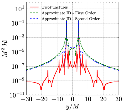
Figure 1: Violation of the constraints for the different sets of initial data considered here for the 2BH0 reference binary.

The evolution of these initial data leads to potentially different tracks and hence waveforms. A comparative of the three cases of initial data considered here (but using the same binary parameters as in Table 1, 2BH0) is given in Fig. 2 where we observe the close match of the second order and “exact” TwoPunctures data in comparison with the first order case. This later difference (already observed in Fig. 1 of Ref. Lousto and Zlochower (2008)) can be in part traced back to the effects of the violations of the Hamiltonian constraint in the initial data that propagates in the numerical grid or is accreted by the black holes. In fact we can observe this effect in the evolution of the individual horizon masses until merger in Fig. 3. That would lead to deviations in their relative tracks explaining the differences in their corresponding waveforms in Fig. 2.

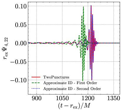
Figure 2: Weyl scalar $\psi_{4}$ extracted at $r_{ex}=113M$ from the evolution of the binary system started with the three different sets of initial data.

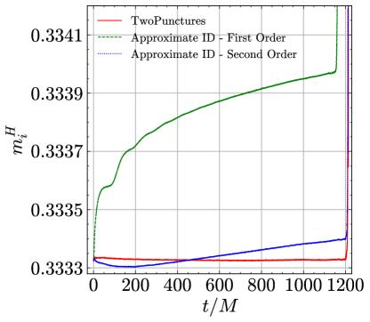
Figure 3: Evolution of the black holes horizon masses starting from the same normalization. Differences are due to different initial violations of the constraints for the sets of approximate initial data considered here.

We supplement the information of the initial data here with another measure of the initial data quality as is the computation of the “binding” energy of the two black holes $E_{b}=M_{ADM}-m$ as the difference of the total ADM mass $M_{ADM}$ and the sum of the horizon masses $m=m_{1}^{H}+m_{2}^{H}$. We compare here its computation via the TwoPuncture numerical solution to the Hamiltonian constraint to the first and second order analytic approximations as given in Eq. (23). For our binary separated by $d=12m$ we find $E_{b}^{N}=-0.00588611$ for the TwoPuncture numerical solution while $E_{b}^{f}=-0.00350055$, and $E_{b}^{s}=-0.00486506$, for the first and second order solutions, representing a 40% and 17% differences, respectively.

IV Three black holes evolutions

We will consider a series of prototypical simulations involving three black holes. In this first exploration we will consider a hierarchical system with the inner binary at an initial separation of $12m=8M$ and a third black hole at separation $30M$. All black holes in this first set will initially have equal masses (as measured by their individual horizons) and no spins, but with different relative orbital orientations. This set up is depicted in Fig. 4.

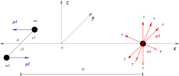
Figure 4: Initial configurations considered for the three black hole evolutions, labeled as 3BH1-5 (3’, 4’, 5’ are quasi-symmetric counterparts).

As a first estimate of the orbital periods we can use the Keplerian expression $P=2\pi/\Omega$ where the orbital frequency is $\Omega=m/r^{3/2}$. Thus for the binary (at $r=12m=8M)$, we find an initial period of $P_{B}=174M$ while for the orbit of the third black hole (at $r=30M)$, a period of $P_{3}=1032M$. From the quasicircular initial orbit Healy et al. (2017) from the third post-Newtonian order (3PN) given in the Table 1 we find $P_{B}^{3PN}=192M$ and $P_{3}^{3PN}=1072M$, respectively. What we measure from the simulation tracks is in close correspondence with those values, i.e. $P_{B}^{NR}\approx 205M$ and $P_{3}^{NR}\approx 1060M$.

In order to chose parameters leading to small initial eccentricities we first consider the inner binary as isolated and apply the quasicircular formulas of Ref. Healy et al. (2017) to obtain the parameters reported in the first column of Table 1 and referred to as 2BH0. Once we have the inner binary parameters we apply the same quasicircular criteria to the outer orbit of the third black hole with an effective spinning black hole having the added masses and angular momentum of the inner binary. In practice this process works to provide low enough eccentricities $(e\lesssim 0.05)$ for our initial study purposes.

IV.1 Three black holes in a hierarchical system

To start exploring this vast parameter space we have chosen to consider two coplanar cases, when the third black hole orbit is corotating with the binary (3BH1) and when it is counter-rotating (3BH2). Those parameters are given in Table 1. We also consider precessing cases with the third black hole momentum perpendicular to the orbital plane of the binary (3BH3) and at $\pm 45$ degrees with respect to that (3BH4 and 3BH5), as depicted in Fig. 4. In all cases we considered the quasicircular orbit of the third black hole with the inner binary as an effective single black hole. The corresponding parameters for these cases are given in Table 2.

Table 2: Initial data parameters for the precessing three black hole cases (3BH3, 3BH4 and 3BH5).

Config	3BH3	3BH4	3BH5
$x_{1}/M$	-9.96709434	-9.95516516	-9.97921106
$y_{1}/M$	3.96401481	3.96401481	3.96401481
$z_{1}/M$	0.00000000	0.00000000	0.00000000
$p_{1}^{x}/M$	-0.05705789	-0.05705825	-0.05705749
$p_{1}^{y}/M$	-0.00036813	-0.01556934	0.01507516
$p_{1}^{z}/M$	-0.02166824	-0.01520121	0.01544329
$m_{1}^{p}/M$	0.32359400	0.32359400	0.32359400
$m_{1}^{H}/M$	0.33332740	0.33332841	0.33332691
$x_{2}/M$	-9.96709434	-9.95516516	-9.97921106
$y_{2}/M$	-3.96401481	-3.96401481	-3.96401481
$z_{2}/M$	0.00000000	0.00000000	0.00000000
$p_{2}^{x}/M$	0.05708188	0.05708152	0.05708228
$p_{2}^{y}/M$	0.00036813	-0.01483308	0.01581142
$p_{2}^{z}/M$	-0.02166824	-0.01520121	0.01544329
$m_{2}^{p}/M$	0.32359400	0.32359400	0.32359400
$m_{2}^{H}/M$	0.33332869	0.33332239	0.33333438
$d/M$	7.92802962	7.92802962	7.92802962
$d_{\rm{spd}}/M$	10.65491937	10.65499784	10.65513690
$x_{3}/M$	19.74820210	19.75949795	19.73672848
$y_{3}/M$	0.00000000	0.00000000	0.00000000
$z_{3}/M$	0.00000000	0.00000000	0.00000000
$p_{3}^{x}/M$	-0.00002398	-0.00002326	-0.00002479
$p_{3}^{y}/M$	0.00000000	0.03040241	-0.03088657
$p_{3}^{z}/M$	0.04333649	0.03040241	-0.03088657
$m_{3}^{p}/M$	0.32910500	0.32906500	0.32906500
$m_{3}^{H}/M$	0.33338457	0.33333346	0.33335498
$M\Omega$	0.00588143	0.00586633	0.00589685
$D/M$	29.7152964	29.7146631	29.7159395

In Fig. 5 we display the extracted waveform of the three black hole simulation 3BH1. The gravitational radiation is completely dominated by the inner binary. The difference with an isolated binary is given by the delay in the merger due to the presence of the third black hole. Similar results are obtained for the 3BH2-5 cases. Another effect is the motion of the binary and its merger product around the center of mass of the triple system, as displayed in Fig. 6. This leads to a mixing of modes as seen by a fixed observer location, but its effects can be disentangled with techniques like those used in Refs. Woodford et al. (2019); Healy and Lousto (2020).

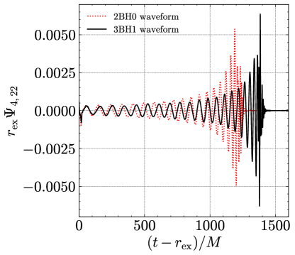
Figure 5: Waveforms generated by the case 3BH1 in comparison with the isolated binary 2BH0.

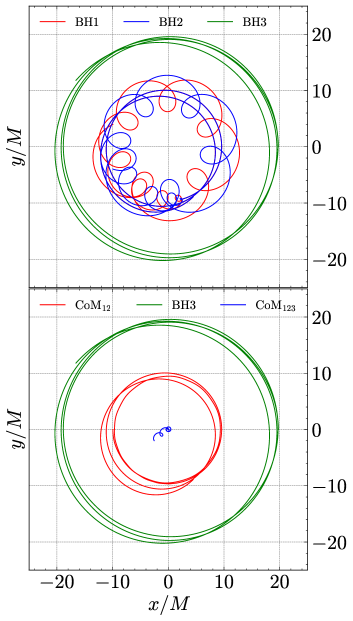
Figure 6: Trajectories of the coplanar case 3BH1 and the evolution of the center of masses of the binary and of the three black holes.

In Fig. 7 we also display the trajectories of the three black holes in the fully precessing case 3BH3 in three dimensions. They clearly display the precession of the third black hole orbital plane over the three orbits of our simulation.

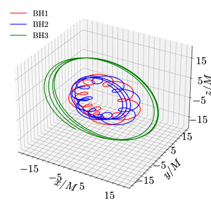
Figure 7: Trajectories of the fully precessing case 3BH3.

In Table 3 we report the merger times of the first five cases studied here. We first note the clear delay of the merger of 3BH1-5 with respect to the isolated binary 2BH0. We then note the relatively weak dependence of the merger times and number of orbits on the orientation of the orbit, at this initial separation of the third hole, $D=30M$.

Table 3: Number of orbits to merger and merger time of the inner binary for different orbital orientations of the third black hole. Cases 3BH1-5

label	$\#$orbits	$t_{\text{merger}}/M$
2BH0	9.949	1216.9
3BH1	10.637	1376.6
3BH2	10.821	1419.9
3BH3	10.523	1341.2
3BH4	10.582	1358.0
3BH5	10.705	1387.5

The other interesting property that we want to study here is the evolution of the eccentricity of the binary due to the presence of the third black hole in a hierarchical orbit around the binary. In Fig. 8 we display the instantaneous Campanelli et al. (2009) eccentricity $e(t)\approx e\cos(\Omega t)\approx d^{2}\ddot{d}/M$, of the inner binary for the three black hole cases 3BH1-5 and the isolated reference binary 2BH0 (B1). We first observe that the amplitude of the eccentricity slightly decrease notably during evolution and presents a modulation with the third black hole orbital frequency.

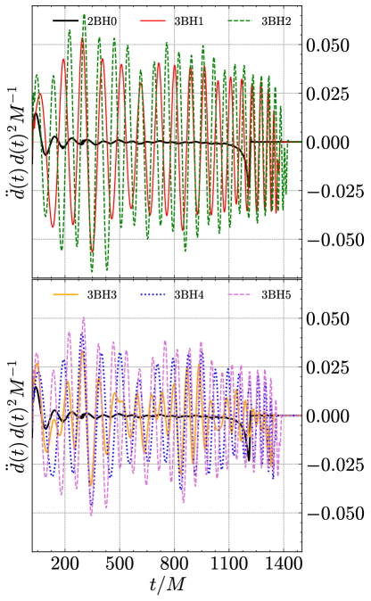
Figure 8: Eccentricity evolution of the inner binary as measured by $d^{2}\ddot{d}(t)$ for the triple black hole cases 3BH1-5 and the isolated reference binary 2BH0.

In order to visualize better the evolution of the eccentricity we take the values of the extremes of oscillations per orbit to model the $e(t)\approx e\cos(\Omega t)$ dependence and extract the values of $e$ per each half orbit of the coplanar cases 3BH1 (corotating orbits) and 3BH2 (counterrotating orbits). The results of this analysis are displayed in Fig. 9.

This is first contrasted with what we expect from an isolated binary on the grounds of the decay of the eccentricity with the instantaneous separation as $\sim d^{1.735}$, found from numerical simulations, see also Fig. 9 in Ref. Lousto et al. (2016). We observe that even if the inner binary starts at a relatively close separation, $12m$, leading to ten orbits before merger compared to the nearly fifty orbits of the simulation analyzed in Ref. Lousto et al. (2016), a general trend towards decrease can be observed. Particularly closer to merger, during the last few orbits, we see a decrease in the eccentricity in as expected on the fact that at those close separations the relative influence of the third black hole should be reduced. We have also verified that the 1PN predictions Peters (1964) that should show a decay of the eccentricity with the instantaneous separation as $\sim d^{19/12}$, give very close results to those displayed in Fig. 9. See also recent 2PN studies in Ref. Datta (2023).

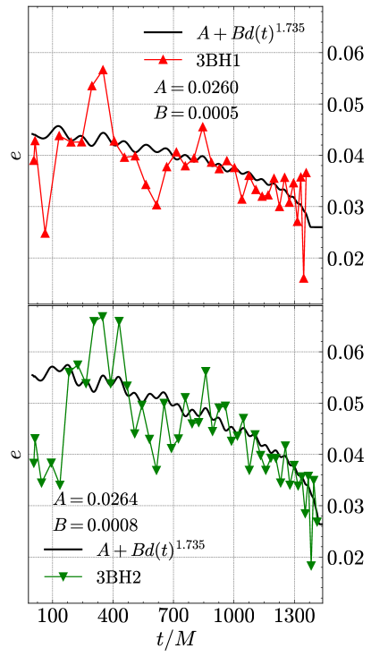
Figure 9: Eccentricity evolution of the inner binary as measured by the amplitude of $d^{2}\ddot{d}(t)$ for the triple black hole cases 3BH1-2 and the expected decay $d^{1.735}$ of Ref. Lousto et al. (2016). (Note the zoom factor $\times 10$ on the right panel).

Another feature that appears in both cases displayed in Fig. 9 is a modulation superposed over an steady decrease of the eccentricity. This modulation has a period of around $\sim 500M$ which seems to correspond to the semi-periods of the third black hole, that we estimated above to be initially of the order of $\approx 1060M$. It also bears resemblance to a beating frequency of the two orbital motions $(\Omega_{2BH}-\Omega_{3BH})/2\approx 468M$.

Finally, we can look at the eccentricity evolution of the orbit of the third black hole. Before merger we can refer its motion around the center of mass of the binary system, as displayed in the bottom of Fig. 6 and then after the merger of the the inner binary to its remnant, as displayed on the right panel of Fig. 10.

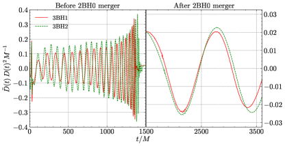
Figure 10: Eccentricity evolution of the outer black hole as measured by the amplitude of $D^{2}\ddot{D}(t)$ for the three coplanar black hole cases 3BH1-2.

We note that the eccentricity measure from the center of mass of the binary seems to grow in time and reaches relatively large values before merger. This seems to be an effect of the use of the coordinates of the center of mass as a reference of this extended system. We note that right after merger the eccentricity measure produces an order of magnitude less eccentricity for the subsequent two orbits and with values more in line with what we expect and found for the inner binary studies above. Qualitatively similar results have been found for the precessing cases 3BH3-5.

IV.2 Numerical convergence

Here we explore the dependence of the previous results on the numerical resolution of the finite difference integrations to perform the evolutions of three black holes. To that end we perform a series of three simulation of the representative case 3BH1, with increasing global resolutions by factors of 1.2, namely the original simulation at n100 resolution and two additional ones at n120 and n144 resolutions. The results of such simulations is summarized in Table 4, were we report the merger times and number of orbits of the inner binary as defined by its trajectories approaching at a distance of $d_{m}=0.7M$ (this corresponds closely to the first appearance of a common apparent horizon within a $\Delta t\sim 5M$, as we verified directly for 3BH1).

Table 4: Convergence of number of orbits and merger time for the 3BH1 configuration using three resolutions. Richardson extrapolation is used to determine convergence order and infinitely extrapolated values. We point out that the difference between different resolutions is smaller than differences between the different configurations.

resolution	$\#$orbits	$t_{\rm{merger}}/M$
n100	10.637	1376.6
n120	10.603	1370.4
n144	10.597	1369.6
Inf. Extrap.	10.596	1369.5
Inf.$-$ n100	-0.041	-7.1
$\%$ difference	-0.387	-0.518
Conv. order	9.51	11.23

We observe that those values align in a convergence order leading to high powers of convergence, as computed by the formulas (5a)-(5c) of Lousto and Healy (2019), still comparable to the expected 8th order convergence from the spatial finite difference stencils used in our integration algorithm. The relevant point here is that the differences of the n100 simulations values we use as a basis to extract conclusions about delays in merger times and number of orbits to merger to its (Richardson’s) extrapolation to infinite resolution is very small compared to the physical changes we observe. We hence conclude they are a numerically reliable result and will keep using this n100 resolution as the standard for the following studies.

IV.3 The Distance dependence to the third black hole

Given the weak sensitivity of the binary evolution with the direction of the third black hole momentum, we will next explore how the merger times and eccentricity evolution of the binary vary versus the initial separation of the outer black hole. For that end we look again for quasicircular effective parameters at different initial separations as given in Table 5.

Table 5: Initial data parameters for coplanar-corotating configurations with a third black hole placed at different distances $D$ from the binary along the $x$-axis, 3BHD1-5.

Config	3BHD1	3BHD2	3BHD3	3BHD4	3BHD5
$x_{1}/M$	-8.28225635	-11.61795003	-13.28540069	-14.95270161	-19.95406346
$y_{1}/M$	3.96401481	3.96401481	3.96401481	3.96401481	3.96401481
$p_{1}^{x}/M$	-0.05705000	-0.05706264	-0.05706503	-0.05706647	-0.05706844
$p_{1}^{y}/M$	-0.02408677	-0.02005564	-0.01867731	-0.01755115	-0.01511026
$m_{1}^{p}/M$	0.32325400	0.32386400	0.32406400	0.32421600	0.32453600
$m_{1}^{H}/M$	0.33335247	0.33333709	0.33334068	0.33333886	0.33335088
$x_{2}/M$	-8.28225635	-11.61795003	-13.28540069	-14.95270161	-19.95406346
$y_{2}/M$	-3.96401481	-3.96401481	-3.96401481	-3.96401481	-3.96401481
$p_{2}^{x}/M$	0.05708976	0.05707712	0.05707474	0.05707329	0.05707133
$p_{2}^{y}/M$	-0.02335051	-0.01931938	-0.01794106	-0.01681489	-0.01437400
$m_{2}^{p}/M$	0.32325400	0.32386400	0.32406400	0.32421600	0.32453600
$m_{2}^{H}/M$	0.33334355	0.33332930	0.33333270	0.33333175	0.33334414
$d/M$	7.92802962	7.92802962	7.92802962	7.92802962	7.92802962
$d_{\rm{spd}}/M$	10.67520743	10.64064151	10.63015429	10.62193283	10.60525218
$x_{3}/M$	16.46307522	23.06578078	26.36782091	29.67012192	39.57796287
$y_{3}/M$	0.00000000	0.00000000	0.00000000	0.00000000	0.00000000
$p_{3}^{x}/M$	-0.00003976	-0.00001448	-0.00000970	-0.00000682	-0.00000288
$p_{3}^{y}/M$	0.04743728	0.03937502	0.03661837	0.03436605	0.02948426
$m_{3}^{p}/M$	0.32823500	0.32968500	0.33014500	0.33048500	0.33116543
$m_{3}^{H}/M$	0.33333394	0.33334810	0.33335404	0.33333988	0.33330813
$M\Omega$	0.00763429	0.00465268	0.00384912	0.00323775	0.00211854
$D/M$	24.7453316	34.6837309	39.6532216	44.6228235	59.5320263

We are interested in studying the effect the third hole has on the inner binary dynamics. In particular how it affects the merger, if prompts or delays it. In Table 6 we give the results of our simulations versus the initial third black hole distance to the binary’s center of mass. We find a clear trend towards the delay of the merger, in both measures, the merger time and the number of orbits as measured by the tracks of the holes and using a definition of merger when the binary distance reaches $d=0.7M$ (which corresponds closely to the formation of a common horizon).

Table 6: Number of orbits to merger and merger time of the inner binary for different initial separation of the third black hole. Cases 3BHD1-5

$D/M$	$\#$orbits	$t_{\text{merger}}/M$
30	10.63	1376.6
35	10.40	1323.6
40	10.25	1292.6
45	10.18	1275.0
60	10.09	1250.5
$\infty$	9.94915	1216.875

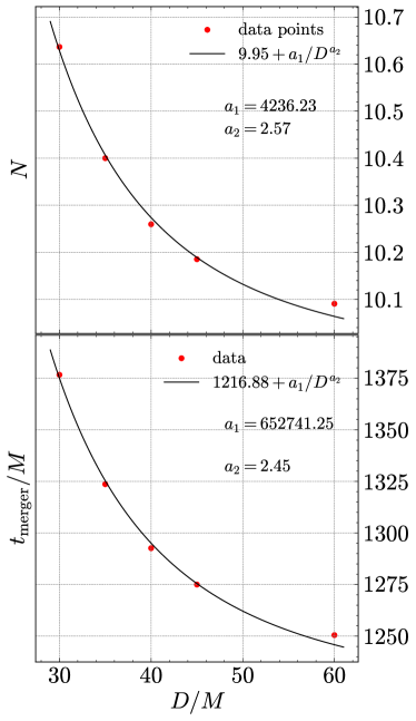
Figure 11: Fit to a functional dependence $2BH0+a1/D^{a2}$.

In order to model the merger delay as a function of the initial distance to the third black hole we consider deviations with respect to the merger time and number of orbits to merger isolated binary, 2BH0. We thus fit a dependence to the data in Table 6 of the form $2BH0+a1/D^{a2}$. The results are displayed in Fig. 11 and lead to a consistent dependence of the form $1/D^{2.5}$.

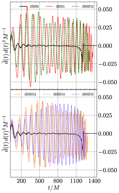
Figure 12: Eccentricity evolution of the inner binary as measured by $d^{2}\ddot{d}(t)$ for the triple black hole cases 3BH1, 3BHD2-5 and the isolated reference binary 2BH0.

We again study the instantaneous eccentricity evolution of the inner binary as we vary the orbital distance of the third black hole. The results are displayed in Fig. 12. While the initial magnitude of the eccentricity is due to the choice of the orbital parameters their evolution shows a trend towards reduction for all cases, particularly very close to merger.

V Conclusions and Discussion

Although full numerical solutions to three black holes initial data have been presented in Refs. Galaviz et al. (2010); Bai et al. (2011); Imbrogno et al. (2023) we found a valid and practical option, validated for the two black hole cases, to provide analytic initial data for prompt use and with enough accuracy for current exploratory studies.

We next revisited the triple black hole scenario to study their merging times and eccentricity evolution. We found that the third black hole delays the merger of the binary by an amount inversely proportional to a power of the distance, $\sim 1/D^{2.5}$. This behavior was not clearly observed in some of the configurations simulated in a previous work Lousto and Zlochower (2008), due to the closeness of the cases studied that lead to a prompt breakdown of the binary, as we also observe here if we start the third black hole closer to $\approx 30M$. We also note here that the $\sim 1/D^{2.5}$ dependence can be associated to a 5th post-Newtonian correction and its leading tidal effects on the inner binary waveforms Flanagan and Hinderer (2008).

A delay in the merger time of the binary due to the presence of the third black hole has also been observed in the Post-Newtonian approximation Galaviz and Bruegmann (2011) considering much larger separations of the binary $(130M-170M)$ and to the third black hole up to $(10\,000M)$, thus representing a complementary study to the one presented here.

The presence of a nearby third black hole also seems to confirm a decay of any residual inner binary eccentricity and to induce a subtle modulation with about a half the period of the third black hole orbit around the binary. Note that in Ref. Naoz et al. (2013) it was studied with post-Newtonian techniques Lousto and Nakano (2008) resonant eccentricity excitation in hierarchical three-body systems, another complementary study to that presented here.

The next natural exploration of 3BH interactions with our formalism involves the inclusion of spins in the inner binary, the unequal mass ratio to consider binaries in the field of a much larger black hole, and the scattering effects of a passing third black hole. Those will be covered in a forthcoming study.

Appendix A Rotation matrix

When we want to study the perturbation of the Hamiltonian constraint at second order we encounter terms of interaction between the momentum P and spin J of the same black hole. Since this perturbative solution requires to choose a specific axis with respect to which we write the spherical harmonics, we need to be able to write the angle between the position r and, for example, the spin in terms of the angular coordinates taken starting from P as $z$ axis.

In order to do so let’s consider the momentum versor $\hat{\textbf{P}}$ and spin versor $\hat{\textbf{J}}$ in a certain coordinate system

$$\hat{\textbf{P}}=\begin{bmatrix}P_{x}\\ P_{y}\\ P_{z}\end{bmatrix}\ \ \ \ \ \ \ \ \hat{\textbf{J}}=\begin{bmatrix}J_{x}\\ J_{y}\\ J_{z}\end{bmatrix}$$ (26)

Let’s call the matrix $R_{G\textbf{P}}$ the matrix that rotates the vector $\hat{\textbf{P}}$ into the vector $\hat{\textbf{z}}$ with

$$\hat{\textbf{z}}=\begin{bmatrix}0\\ 0\\ 1\end{bmatrix}$$ (27)

This matrix is constructed through

$$R_{GP}=I+V+\frac{V\cdot V}{1+C}$$ (28)

where

$$V=\begin{bmatrix}0&-V_{z}&V_{y}\\ V_{z}&0&-V_{x}\\ -V_{y}&V_{x}&0\end{bmatrix}$$ (29)

and

$$\textbf{V}=\hat{\textbf{P}}\times\hat{\textbf{z}}\ \ \ \ \ \ \ \ C=\hat{\textbf{P}}\cdot\hat{\textbf{z}}$$ (30)

This is also the matrix that transforms the coordinates of a given vector in the reference system G to the one in which the z axis is aligned along $\hat{\textbf{P}}$ (which we call P).

Analogously we find $R_{G\textbf{J}}$ and $R_{G\textbf{J}\times\textbf{P}}$.

Once we have these matrices we can combine them to find $R_{\textbf{P}\textbf{J}}$, $R_{\textbf{P}\textbf{J}\times\textbf{P}}$ and $R_{\textbf{J}\textbf{J}\times\textbf{P}}$.

Now let’s consider for example the unit vector $\hat{\textbf{n}}$ which has coordinates

$$\hat{\textbf{n}}=\begin{bmatrix}n_{xP}\\ n_{yP}\\ n_{zP}\end{bmatrix}$$ (31)

in the P system.

Then the coordinates of $\hat{\textbf{n}}$ in the J system are

$$\begin{bmatrix}n_{xJ}\\ n_{yJ}\\ n_{zJ}\end{bmatrix}=R_{\textbf{P}\textbf{J}}\begin{bmatrix}n_{xP}\\ n_{yP}\\ n_{zP}\end{bmatrix}$$ (32)

In particular we are only interested in the 3rd coordinate $n_{zJ}$ which is

$$n_{zJ} =R_{\textbf{P}\textbf{J}}^{31}n_{xP}+R_{\textbf{P}\textbf{J}}^{32}n_{yP}+R_{\textbf{P}\textbf{J}}^{33}n_{zP}$$

$$=\sin{\theta_{\textbf{P}}}(R_{\textbf{P}\textbf{J}}^{31}\cos{\phi_{\textbf{P}}}+R_{\textbf{P}\textbf{J}}^{32}\sin{\phi_{\textbf{P}}})+R_{\textbf{P}\textbf{J}}^{33}\cos{\theta_{\textbf{P}}}$$

Applying this procedure for all the cases we need we finally obtain

$$\begin{split}n_{zJ}=&\sin{\theta_{\textbf{P}}}(R_{\textbf{P}\textbf{J}}^{31}\cos{\phi_{\textbf{P}}}+R_{\textbf{P}\textbf{J}}^{32}\sin{\phi_{\textbf{P}}})\\ &+R_{\textbf{P}\textbf{J}}^{33}\cos{\theta_{\textbf{P}}}\\ n_{z\textbf{J}\times\textbf{P}}=&\sin{\theta_{\textbf{P}}}(R_{\textbf{P}\textbf{J}\times\textbf{P}}^{31}\cos{\phi_{\textbf{P}}}+R_{\textbf{P}\textbf{J}\times\textbf{P}}^{32}\sin{\phi_{\textbf{P}}})\\ &+R_{\textbf{P}\textbf{J}\times\textbf{P}}^{33}\cos{\theta_{\textbf{P}}}\\ n_{z\textbf{J}\times\textbf{P}}=&\sin{\theta_{\textbf{J}}}(R_{\textbf{J}\textbf{J}\times\textbf{P}}^{31}\cos{\phi_{\textbf{J}}}+R_{\textbf{J}\textbf{J}\times\textbf{P}}^{32}\sin{\phi_{\textbf{J}}})\\ &+R_{\textbf{J}\textbf{J}\times\textbf{P}}^{33}\cos{\theta_{\textbf{J}}}\end{split}$$ (34)

To determine let’s say the angle $\phi_{\textbf{P}}$ (an analogous argument holds for $\phi_{\textbf{J}}$) we make use of the matrix $R_{G\textbf{P}}$ as follows. Let’s say that in in the system of coordinates $G$ the coordinates of $\hat{\textbf{n}}$ are

$$\hat{\textbf{n}}=\begin{bmatrix}n_{xG}\\ n_{yG}\\ n_{zG}\end{bmatrix}$$ (35)

Then we have,

$$\begin{split}\tan{\phi_{\textbf{P}}}=&{\frac{\sin{\phi_{\textbf{P}}}}{\cos{\phi_{\textbf{P}}}}}=\frac{(R_{G\textbf{P}}\cdot\textbf{n})_{x}}{(R_{G\textbf{P}}\cdot\textbf{n})_{y}}\end{split}$$ (36)

From this we can obtain $\phi_{\textbf{P}}$ (and $\phi_{\textbf{J}}$).

References

- Gayathri et al. (2022) V. Gayathri, J. Healy, J. Lange, B. O’Brien, M. Szczepanczyk, I. Bartos, M. Campanelli, S. Klimenko, C. O. Lousto, and R. O’Shaughnessy, Nature Astron. 6, 344 (2022), arXiv:2009.05461 [astro-ph.HE] .
- Yu et al. (2020) H. Yu, S. Ma, M. Giesler, and Y. Chen, Phys. Rev. D 102, 123009 (2020), arXiv:2007.12978 [gr-qc] .
- Dall’Amico et al. (2021) M. Dall’Amico, M. Mapelli, U. N. Di Carlo, Y. Bouffanais, S. Rastello, F. Santoliquido, A. Ballone, and M. A. Sedda, Mon. Not. Roy. Astron. Soc. 508, 3045 (2021), arXiv:2105.12757 [astro-ph.HE] .
- Martinez et al. (2022) M. A. S. Martinez, C. L. Rodriguez, and G. Fragione, Astrophys. J. 937, 78 (2022), arXiv:2105.01671 [astro-ph.SR] .
- Ryu et al. (2022) T. Ryu, R. Perna, and Y. Wang, Mon. Not. Roy. Astron. Soc. 516, 2204 (2022), arXiv:2206.00603 [astro-ph.HE] .
- Campanelli et al. (2008) M. Campanelli, C. O. Lousto, and Y. Zlochower, Phys. Rev. D77, 101501(R) (2008), arXiv:0710.0879 [gr-qc] .
- Lousto and Zlochower (2008) C. O. Lousto and Y. Zlochower, Phys. Rev. D77, 024034 (2008), arXiv:0711.1165 [gr-qc] .
- Lousto and Nakano (2008) C. O. Lousto and H. Nakano, Class. Quant. Grav. 25, 195019 (2008), arXiv:0710.5542 [gr-qc] .
- Laguna (2004) P. Laguna, Phys. Rev. D 69, 104020 (2004), gr-qc/0310073 .
- Galaviz et al. (2010) P. Galaviz, B. Bruegmann, and Z. Cao, Phys. Rev. D 82, 024005 (2010), arXiv:1004.1353 [gr-qc] .
- Bowen and York (1980) J. M. Bowen and J. W. York, Jr., Phys. Rev. D21, 2047 (1980).
- Zlochower et al. (2005) Y. Zlochower, J. G. Baker, M. Campanelli, and C. O. Lousto, Phys. Rev. D72, 024021 (2005), arXiv:gr-qc/0505055 .
- Brandt and Brügmann (1997) S. Brandt and B. Brügmann, Phys. Rev. Lett. 78, 3606 (1997), gr-qc/9703066 .
- Ansorg et al. (2004) M. Ansorg, B. Brügmann, and W. Tichy, Phys. Rev. D70, 064011 (2004), gr-qc/0404056 .
- Thornburg (2004) J. Thornburg, Class. Quant. Grav. 21, 743 (2004), gr-qc/0306056 .
- Campanelli et al. (2007) M. Campanelli, C. O. Lousto, Y. Zlochower, B. Krishnan, and D. Merritt, Phys. Rev. D75, 064030 (2007), gr-qc/0612076 .
- Schnetter et al. (2004) E. Schnetter, S. H. Hawley, and I. Hawke, Class. Quant. Grav. 21, 1465 (2004), gr-qc/0310042 .
- Campanelli et al. (2009) M. Campanelli, C. O. Lousto, H. Nakano, and Y. Zlochower, Phys. Rev. D79, 084010 (2009), arXiv:0808.0713 [gr-qc] .
- Alcubierre et al. (2005) M. Alcubierre et al., Phys. Rev. D72, 044004 (2005), gr-qc/0411149 .
- Campanelli and Lousto (1999) M. Campanelli and C. O. Lousto, Phys. Rev. D59, 124022 (1999), arXiv:gr-qc/9811019 [gr-qc] .
- Lousto and Zlochower (2007) C. O. Lousto and Y. Zlochower, Phys. Rev. D76, 041502(R) (2007), gr-qc/0703061 .
- Healy et al. (2017) J. Healy, C. O. Lousto, H. Nakano, and Y. Zlochower, Class. Quant. Grav. 34, 145011 (2017), arXiv:1702.00872 [gr-qc] .
- Woodford et al. (2019) C. J. Woodford, M. Boyle, and H. P. Pfeiffer, Phys. Rev. D100, 124010 (2019), arXiv:1904.04842 [gr-qc] .
- Healy and Lousto (2020) J. Healy and C. O. Lousto, Phys. Rev. D 102, 104018 (2020), arXiv:2007.07910 [gr-qc] .
- Lousto et al. (2016) C. O. Lousto, J. Healy, and H. Nakano, Phys. Rev. D93, 044031 (2016), arXiv:1506.04768 [gr-qc] .
- Peters (1964) P. C. Peters, Phys. Rev. 136, B1224 (1964).
- Datta (2023) S. Datta, (2023), arXiv:2306.12522 [gr-qc] .
- Lousto and Healy (2019) C. O. Lousto and J. Healy, Phys. Rev. D100, 104039 (2019), arXiv:1908.04382 [gr-qc] .
- Bai et al. (2011) S. Bai, Z.-J. Cao, W.-B. Han, C.-Y. Lin, H.-J. Yo, and J.-P. Yu, J. Phys. Conf. Ser. 330, 012016 (2011), arXiv:1203.6185 [gr-qc] .
- Imbrogno et al. (2023) M. Imbrogno, C. Meringolo, and S. Servidio, Class. Quant. Grav. 40, 075008 (2023), arXiv:2108.01392 [gr-qc] .
- Flanagan and Hinderer (2008) E. E. Flanagan and T. Hinderer, Phys. Rev. D77, 021502 (2008), arXiv:0709.1915 [astro-ph] .
- Galaviz and Bruegmann (2011) P. Galaviz and B. Bruegmann, Phys. Rev. D83, 084013 (2011), arXiv:1012.4423 [gr-qc] .
- Naoz et al. (2013) S. Naoz, B. Kocsis, A. Loeb, and N. Yunes, Astrophys. J. 773, 187 (2013), arXiv:1206.4316 [astro-ph.SR] .