Quantum information entropies for solitonic systems

Abstract

Particle with position-dependent mass is a useful concept in the context of semiconductor physics. We study a particle with the solitonic mass distribution in two different forms of potential: the quartic and the symmetric potential. We estimate the Shannon entropy and Fisher information associated with the ground state of particle in these two scenarioes by obtaining the wave-function from Zhu-Kroemer equation. The ground state of the particle in each case satisfies the Bialynicki-Birula–Mycielski inequality. Upon comparing all four models under consideration, we have observed that the Shannon entropy is greater for the solitonic mass distribution when it is subjected to a quartic potential.

I Introduction

Solitons, also known as solitary waves, encompass a range of physical phenomena, including shock waves in sound waves and ultra-short optical pulses in optical fibers [1]. From a mathematical perspective, solitons can be understood as localized solutions to partial differential equations that describe nonlinear systems with infinite degrees of freedom [2]. The groundbreaking contributions of Feynman have significantly influenced and propelled the field of Quantum information processing [3]. Consequently, the study of solitons holds great importance in the realm of Quantum information processing. More precisely, the study of solitons are profound in the field of Quantum communication [4, 5, 6]. Solitons are distinct from elementary particles that emerge from quantized wave-like excitations of the fields [7]. Their characteristics are primarily determined by classical equations. This research took place during the early stages of quantum field theory in the late 1960s. There exist important connections between the solitons of a theory and the wave-like fields that satisfy the linearized field equations. Quantizing the latter results in states of elementary particles, with the interactions between these particles being governed by the nonlinear components [2]. Initially, in regions far from the soliton, the field progressively tends towards the vacuum state, adhering to the rate determined by the linearized field equation. Therefore, if the linearized equation lacks a mass term, leading to the existence of massless elementary particles, the impact of the soliton will extend over a considerable distance, diminishing inversely as distance increases. This comprehension has implications for multiple facets of quantum field theory within condensed matter setups [8]. Initially, in quantum mechanics, the Schrodinger equation focused on physical systems with a constant effective mass. However, advancements in condensed matter physics presented a new challenge: the existence of non-relativistic particles that exhibit a position-dependent effective mass. Subsequently, the study of systems with position-dependent effective mass has garnered significant attention from researchers due to its wide range of applications.

In conjunction with the concept of position-dependent effective mass arises the theory of communication, formally known as the Information theory proposed by Claude Shannon around mid-1900s. Entropy, as a measurable physical property, is commonly associated with a state of disorder, randomness, or uncertainty. In the context of thermodynamics [9], entropy represents a measure of irreversibility within a physical system. However, it is important to note that this concept of entropy differs from information entropy, which is the focus of our interest. Several parameters highlight the distinctions between thermodynamic entropy and information entropy. Thermodynamic entropy considers the number of possible structural arrangements within a system, while informational entropy pertains to choices made within a communication system. In recent times, there has been a growing interest in utilizing information-theoretic measures for quantum systems. Notably, entropic uncertainty relations have been explored as alternatives to the Heisenberg uncertainty principle [10]. Furthermore, Shannon entropy [11] and entropic uncertainty relations find applications in various areas. These include the study of squeezed localization [12], fractional revivals [13, 14], and reconstruction of charge and momentum densities in atomic and molecular systems using maximum entropy procedures [15]. Additionally, Shannon entropy [11] finds utility in Measure theory [16], the study of open quantum systems involving Markov chains [17], machine learning for decision tree algorithms, and Bayesian inference [18].

The Fisher information, also referred to as Fisher’s entropy, is a fascinating concept that emerges from communication theory and is recognized as a precursor to Shannon entropy [19]. In the quantum domain, Fisher information is inherently connected to the uncertainty connected with measurement, as explained in references [20]. Essentially, Fisher’s information measures the information content carried by a specific observable concerning a parameter, while considering its inherent probability [19].

This article is structured as follows: In section II, we provide an overview of Shannon entropy, entropic uncertainty, and Fisher’s information measure . In section III, we provide a detailed explanation of the quantum mechanics of position-dependent mass. In section IV, V, we calculate Shannon and Fisher’s information measure for different solitonic systems and discuss the results in section VI. We have computed all calculations for systems in their ground state and by considering the convention $\hbar=c=1$.

II Shannon entropy and Fisher’s information measure - A bird’s eye view

In the realm of information theory, Shannon entropy, originally introduced by Claude Shannon in 1948 in his publication ‘A Mathematical Theory of Communication [11], represents an average rate of information generation from a stochastic data source. A higher value of Shannon entropy implies that a new value from the process provides more information. Mathematically, for a given distribution function $p_{i}$, Shannon entropy can be defined as follows [11]:

$$S=-\sum p_{i}\text{ln}(p_{i}).$$ (1)

Shannon entropy was not derived from pre-established assumptions but rather developed as a means to quantify the uncertainty principle. It bears a resemblance to Gibbs entropy and is occasionally referred to as ”Boltzmann-Gibbs-Shannon” entropy [21]. Shannon entropy can be conceptualized as the measure of uncertainty within a probability distribution connected to an information source. In the context of a given probability distribution in position space, Shannon entropy in the $n$th state is defined as.

$$S_{x}=-\int_{-\infty}^{\infty}dx\bigg{[}(\psi_{n}(x))^{2}\text{ln}(\psi_{n}(x))^{2}\bigg{]}.$$ (2)

In the reciprocal space (momentum representation), Shannon entropy in the $n$th state is defined by

$$S_{k}=-\int_{-\infty}^{\infty}dk\bigg{[}(\phi_{n}(k))^{2}\text{ln}(\phi_{n}(k))^{2}\bigg{]},$$ (3)

where,

$$\phi_{n}(k)=\frac{1}{\sqrt{2\pi}}\int_{-\infty}^{\infty}e^{-ikx}\psi_{n}(x)dx.$$ (4)

While the uncertainty principle deals with the limits of measurement in quantum mechanics, Shannon entropy deals with the quantification of information in a probabilistic framework. However, there is a conceptual similarity between the two in terms of the idea of uncertainty and the limits of knowledge or measurement. In quantum mechanics, the uncertainty principle implies that there are inherent limits to the simultaneous knowledge of certain pairs of complementary properties, such as position and momentum, or energy and time. This uncertainty arises from the wave-particle duality of quantum systems and the probabilistic nature of quantum measurements. Shannon entropy, on the other hand, provides a measure of uncertainty or unpredictability in a probability distribution. It quantifies the average amount of information needed to describe or predict the outcomes of a random variable. High entropy implies higher uncertainty or unpredictability, while low entropy implies lower uncertainty or greater predictability. Although these concepts are not directly connected, they both reflect the fundamental limitations on our ability to precisely know or predict certain aspects of physical systems. The uncertainty principle sets limits on the simultaneous knowledge of complementary properties in quantum mechanics, while it quantifies the uncertainty or information content of random variables in a probabilistic framework. This is been briefly discussed in [22, 23], which can be represented as

$$S_{x}+S_{k}\geq D(1+\text{ln}\pi),$$ (5)

where $D$ denotes the dimension of the system. The computation of Shannon entropy analytically is challenging due to the presence of logarithmic terms in the integrals, especially considering the system’s dimension. As a result, it has only been determined for specific lower-energy states of certain systems such as the Harmonic oscillator [24], the Pöschl–Teller potential [25], the Morse potential [26], and highly excited states of the Coulomb potential [27].

The foundation of the second law of thermodynamics lies in the concept of entropy [28]. According to this law, the overall entropy of a closed system increases as time progresses and approaches a maximum value in the limit of infinite time. In its classical formulation, entropy is applicable to systems in equilibrium and is defined by Clausius and others (see ref.[29]), can be demonstrated by

$$dS=\frac{\delta Q}{T}.$$ (6)

As mentioned earlier, when viewed through the lens of information theory, entropy serves as a metric for the level of disorder within a system [22]. Consequently, the entropy of a thermodynamic system escalates as the count of accessible microstates for the system expands. In the realm of information theory, there exists an alternative form of information known as Fisher information ($F$) [30]. It is of the form,

$$F=\sum_{i=1}^{m}\frac{1}{p_{i}}\bigg{[}\frac{dp_{i}}{di}\bigg{]}^{2},$$ (7)

where, $p_{i}$ denotes the probability density for finding the system in micro-state $i$. In the context of a specific thermodynamic system [9], an increase in the number of microstates leads to a corresponding increase in entropy. This occurs because the system becomes more disordered, resulting in higher entropy. For instance, if the system occupies a single microstate, the probability density function exhibits a steep slope around that state, indicating high Fisher information. Conversely, if the system exists in numerous states with approximately equal probabilities, the probability density function becomes flat, with a nearly zero slope and Fisher information. Therefore, Fisher information serves as a measure of order within the system, representing a scenario where the system exists predictably in one or a few high-probability microstates. It should be noted that despite the resemblance of equations (1) and (7), these two quantities do not measure the same property of the system. Shannon entropy is determined by the probability density function, while Fisher information depends on the derivative of the probability density function, representing its slope. Consequently, it can be regarded as a global property, while Fisher information can be considered a local property relative to the probability density function. Therefore, Fisher information and Shannon entropy are not analogous to each other. Fisher’s information for an observable $\zeta$ is defined as

$$F_{\zeta}=\int_{-\infty}^{\infty}d\zeta\bigg{[}\rho(\zeta)\bigg{(}\frac{d}{d\zeta}\text{ln}(\rho(\zeta))\bigg{)}^{2}\bigg{]}>0,$$ (8)

We calculate Fisher’s information for an observable $\zeta$ whose probability density is $|\psi(\zeta,t)|^{2}$ is given by

$$F_{\zeta}=\int_{-\infty}^{\infty}d\zeta\bigg{[}(\psi(\zeta,t))^{2}\bigg{(}\frac{d}{d\zeta}\text{ln}(\psi(\zeta,t))^{2}\bigg{)}^{2}\bigg{]}>0,$$

However, in one dimensional stationary quantum systems (solitonic systems), at position space, $\rho(\zeta)=|\psi(\zeta,t)|^{2}\approx|\psi(\zeta)|^{2}$, is the probability density. It can be obtained by approximating $\psi(\zeta,t)$ to $\psi(\zeta)$.

$$F_{\zeta}=\int_{-\infty}^{\infty}d\zeta\bigg{[}(\psi(\zeta))^{2}\bigg{(}\frac{d}{d\zeta}\text{ln}(\psi(\zeta))^{2}\bigg{)}^{2}\bigg{]}.$$ (9)

Similarly, we compute Fisher information for the same soliton in the momentum space.

$$F_{k}=\int_{-\infty}^{\infty}dk\bigg{[}(\phi(k,t))^{2}\bigg{(}\frac{d}{dk}\text{ln}(\phi(k,t))^{2}\bigg{)}^{2}\bigg{]},$$ (10)

Implementing the same approximation as before we get Fisher information as

$$F_{k}=\int_{-\infty}^{\infty}dk\bigg{[}(\phi(k))^{2}\bigg{(}\frac{d}{dk}\text{ln}(\phi(k))^{2}\bigg{)}^{2}\bigg{]}.$$ (11)

where, $\phi(k)=\frac{1}{\sqrt{2\pi}}\int_{-\infty}^{\infty}e^{-ik\zeta}\psi(\zeta)d\zeta$. Uncertainty, in the context of Fisher information, refers to the degree of imprecision or lack of knowledge about the true value of a parameter. It captures the spread or variability in the estimates obtained from different samples or measurements. It measures the uncertainty or randomness associated with parameter estimation based on observed data, with higher entropy implying lower uncertainty and better estimation performance. This is represented as follows

$$F_{\zeta}F_{k}\geq 4\hbar^{2}.$$ (12)

where, $\hbar$ is reduced Planck’s constant.

III Quantum mechanics with position dependent mass

In standard quantum mechanics, the mass of a particle is typically treated as a constant. However, there are certain physical systems where the mass of a particle can depend on its position within the system. This introduces an additional complexity in the mathematical formalism of quantum mechanics, but it can be accommodated using position-dependent mass quantum mechanics. The Schrodinger equation, which describes the behavior of quantum systems, needs to be modified to account for the position-dependent mass. The general form of the Schrodinger equation for a particle with position-dependent mass is

$$\frac{-\hbar^{2}}{2m(x)}\frac{d^{2}\psi}{dx^{2}}+V(x)\psi=E\psi,$$ (13)

where, $E$ is the energy, $\psi(x)$ is a wave function and $V(x)$ is the potential energy. The position-dependent mass function m(x) introduces a spatial dependence in the kinetic energy term of the Schrodinger equation. This means that the behavior of the particle can vary depending on its position within the system. Different choices for $m(x)$ can lead to a variety of interesting physical phenomena. Throughout the sections we use the mass distribution to be

$$m(x)=\frac{m_{0}}{1+x^{2}}.$$ (14)

Thus, for a position dependent mass, the kinetic energy term ($\hat{T}$) of Schrodinger equation eq. (13) is modified as follows

$$\hat{T}=\frac{-\hbar^{2}}{2\sqrt{m(x)}}\frac{d^{2}}{dx^{2}}\frac{1}{\sqrt{m(x)}}.$$ (15)

The Hamiltonian operator ($\hat{H}$), which describes the energy of a stationary system (solitonic system) in quantum mechanics, can be expressed in the following manner

$$\hat{H}=\frac{-\hbar^{2}}{2\sqrt{m(x)}}\frac{d^{2}}{dx^{2}}\frac{1}{\sqrt{m(x)}}+V(x).$$ (16)

The Schrodinger equation modifies as

$$\frac{-\hbar^{2}}{2m}\frac{d^{2}\psi(x)}{dx^{2}}+\frac{-\hbar^{2}}{2}\frac{m^{\prime}(x)}{m(x)^{2}}\frac{d\psi(x)}{dx}+\Bigg{[}\frac{\hbar^{2}}{4}\frac{m^{\prime\prime}(x)}{m(x)^{2}}-\\ \frac{3\hbar^{2}}{8}\frac{m^{\prime}(x)^{2}}{m(x)^{3}}+V(x)\Bigg{]}\psi(x)=E\psi(x).$$ (17)

This differential equation [eq.(17)] is derived by Zhu and Kroemer [31] and is used in the context of semiconductor physics to explore the electronic properties of semiconductor devices. In the next section, we shall discuss Shannon and Fisher’s information measure for different solitonic systems. The motive of this particular work is from the context of solitons in field theory, where we look for time-independent, finite energy, and localized solutions. The majority of research on solitons focuses on theoretical analyses of soliton solutions in quantum field theories that are not applicable to describing our physical universe. When considering particle physics models that accurately represent our world, solitons often possess unconventional properties such as exotic magnetic monopole charges [2], making them relatively heavy. These applications of solitons represent only a small portion of the extensive literature on solitons. Moreover, there are exceptional cases, like the description of quarks and leptons through a dual electromagnetic gauge group [2] using a magnetic monopole framework, which is even rarer in the soliton literature.

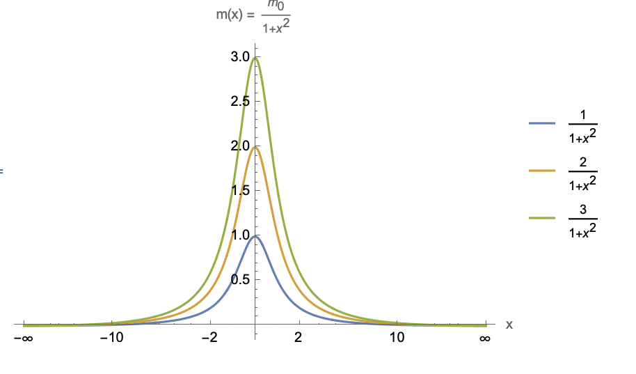
Figure 1: Solitonic mass distribution for constant $m_{0}$

IV Solitons in a Quartic Potential

The double well potential also known as the Quartic potential, holds significant importance in quantum mechanics, quantum field theory, and other other fields for investigating different physical phenomena and mathematical properties. The symmetric well potential is ubiquitous as it serves as a model to illustrate the concept of instantons [2] and Feynman path integral formulation in quantum mechanics [32]. Solitons in quartic potential are formed by the interplay between self-phase modulation and anomalous second- and fourth-order dispersion [33]. This has a widespread application in the field of optical communication [34, 35], such as shape in variance in nonlinear wave packets which enhances optical communication. Recent notable achievements in this area have shown promising outcomes in terms of the potential observation of localized quartic solitons within specifically engineered slot wave guides based on silicon [36]. This is been observed in the case of quartic solitons with a mass distribution of $\frac{m_{0}}{1+x^{2}}$, thus studying the quantum information entropies for the same will help us to understand it much better [37]. The given solitonic mass distribution and well-known quartic potential with parameters $a$ and $b$ can be written as

$$V(x)=ax^{2}+bx^{4},b>0,$$ (18)

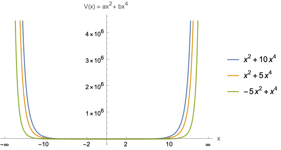
Figure 2: Quartic potential for different values of $a$ and $b$.

.

IV.1 Constant Mass

We start by calculating wave function for this system for constant mass (i.e., $m=m_{0}$), Schrodinger equation for this system is simplified as follows

$$\frac{d^{2}\psi(x)}{dx^{2}}+\bigg{[}A-Bx^{2}-Cx^{4}\bigg{]}\psi(x)=0,$$ (19)

where, $A=\frac{2m_{0}E}{\hbar^{2}},B=\frac{2m_{0}a}{\hbar^{2}},C=\frac{2m_{0}b}{\hbar^{2}}$. The wave function is computed (briefly discussed in VII.1) and is given by

$$\psi(x)=\sqrt{\frac{A}{\pi}}\text{exp}\bigg{[}\frac{-A}{2}x^{2}\bigg{]},$$ (20)

In reciprocal space we can write the wave function as

$$\phi(k)=\frac{1}{\sqrt{\pi}}\text{exp}\bigg{[}\frac{-k^{2}}{2A}\bigg{]}.$$ (21)

IV.1.1 Shannon’s entropy

According to Bonn [38], the statistical interpretation of the quantum system, which describes the probability of finding the particle in the state $\psi(x,t)$ between the spatial interval $x$ and $x+dx$ describes as $|\psi(x,t)|^{2}\approx|\psi(x)|^{2}$. Shannon’s entropy in position space ($S_{x}$) is given by

$$S_{x}=-\int_{-\infty}^{\infty}|\psi(x)|^{2}\text{ln}[|\psi(x)|^{2}]dx,$$ (22)

and we obtain the value for $S_{x}$ as

$$S_{x}=\sqrt{\frac{A}{\pi}}\bigg{(}\frac{1}{2}-\text{ln}\bigg{[}\frac{A}{\pi}\bigg{]}\bigg{)}.$$ (23)

In reciprocal space, it is given by $S_{k}$

$$S_{k}=-\int_{-\infty}^{\infty}|\phi(k)|^{2}\text{ln}[|\phi(k)|^{2}]dk,$$ (24)

where $D$ is the dimension of the spatial coordinates of the system. and we obtain the value for $S_{k}$ as

$$S_{k}=\sqrt{\frac{A}{\pi}}\bigg{(}\frac{1}{2}+\text{ln}\pi\bigg{)},$$ (25)

such that,

$$S_{x}+S_{k}\geq D(1+\text{ln}\pi).$$ (26)

where $D$ is the dimension of the spatial coordinates of the system. The numerical study of Shannon entropy was carried out considering the eigenfunctions at the position and momentum space, as well as the definition of Shannon entropy, i.e. eq. (24) and eq. (22). The numerical result of Shannon entropy for constant mass is presented in the following table:

$A$	$S_{x}$	$S_{k}$	$S_{x}+S_{k}$	$1+\text{ln}\pi$
3.5	0.4137	1.7359	2.1496	2.1447
3.6	0.3894	1.7605	2.1499	2.1447
3.7	0.3650	1.7848	2.1498	2.1447
3.8	0.3406	1.8088	2.1494	2.1447
3.9	0.3161	1.8324	2.1485	2.1447
4.0	0.2915	1.8558	2.1473	2.1447
4.2	0.2424	1.9016	2.1448	2.1447

Table 1: Numerical results of the Shannon entropy

IV.1.2 Fisher’s Information measure

For an observable $x$, Fisher information ($F_{x}$) is given by

$$F_{x}=\int_{-\infty}^{\infty}|\psi(x)|^{2}\bigg{[}\frac{d}{dx}\text{ln}|\psi(x)|^{2}\bigg{]}^{2}dx>0,$$ (27)

and we obtain the value for $F_{x}$ as

$$F_{x}=\frac{2A^{\frac{3}{2}}}{\sqrt{\pi}}.$$ (28)

In reciprocal space, Fisher information for an observable $k$, ($F_{k}$) is given by

$$F_{k}=\int_{-\infty}^{\infty}|\phi(k)|^{2}\bigg{[}\frac{d}{dk}\text{ln}|\phi(k)|^{2}\bigg{]}^{2}dk>0,$$ (29)

and we obtain the value for $F_{k}$ as

$$F_{k}=\frac{2}{\sqrt{A\pi}}.$$ (30)

Let us also remember that the standard deviation of the position and momentum measures is given respectively by

$$\sigma^{2}_{x}=<x^{2}>-<x>^{2},$$ (31)

$$\sigma^{2}_{k}=<k^{2}>-<k>^{2}.$$ (32)

where, $<x>,<k>,<x^{2}>,<k^{2}>$ are the expected values of $x,k,x^{2},k^{2}$ respectively. Using the definitions of Fisher information given in eq. (8) and eq. (10) and standard deviations given in eq. (31) and eq. (32), we present the numerical result of Fisher’s information measure for mass distribution is presented in the following table:

$A$	$F_{x}$	$F_{k}$	$\sigma^{2}_{x}$	$\sigma^{2}_{k}$	$F_{x}\cdot F_{k}$
3.5	7.386	0.6029	0.1507	1.846	4.453
3.6	7.704	0.5945	0.1486	1.926	4.580
3.7	8.028	0.5864	0.1466	2.007	4.707
3.8	8.356	0.5786	0.1447	2.089	4.834
3.9	8.688	0.5711	0.1428	2.172	4.962
4.0	9.024	0.5640	0.1410	2.256	5.089
4.2	9.709	0.5504	0.1376	2.427	5.344

Table 2: Results for the uncertainty relation and Fisher information measure

Figure 3: Fisher’s information measure for soliton in position space (constant mass) in quartic potential.

Figure 4: Fisher’s information measure for soliton in momentum space (constant mass) in quartic potential.

Consequently, by examining the results of the standard deviation, the Heisenberg uncertainty principle was explored, leading to the derivation of the following relationships,

$$F_{x}=4\sigma^{2}_{k},$$ (33)

$$F_{k}=4\sigma^{2}_{x},$$ (34)

Heisenberg uncertainty principle is written as

$$F_{x}F_{k}\geq 4\hbar^{2}.$$ (35)

IV.2 Mass distribution

We consider the mass distribution to be $m(x)=\frac{m_{0}}{1+x^{2}}$. For the sake of simplicity, we take the values of $a$ and $b$ to be unity. Thus the modified potential can be read as,

$$V(x)=x^{2}+x^{4}.$$ (36)

The Schrodinger equation for the given mass distribution is simplified as,

$$\frac{d^{2}\psi}{dx^{2}}-\frac{2m_{0}}{\hbar^{2}}x^{2}\psi=\frac{-2m_{0}E}{\hbar^{2}}\frac{1}{1+x^{2}}\psi,$$ (37)

The wave function is computed (briefly discussed in VII.1) and is given by

$$\psi(x)=\frac{A}{(1+x^{2})^{1/4}}\text{exp}\bigg{[}\frac{-x^{2}}{2(1+x^{2})}\bigg{]}.$$ (38)

In reciprocal space, we can write the wave function as

$$\phi(k)=\frac{A}{\sqrt{2}}\exp\left(\frac{-k^{2}}{2}-ik\right).$$ (39)

where $A$ is a constant. This computation is carried out by assuming the values of $m_{0}$ to be $1$.

IV.2.1 Shannon Entropy

Shannon’s entropy in position space ($S_{x}$) is given by

$$S_{x}=-\int_{-\infty}^{\infty}|\psi(x)|^{2}\text{ln}|\psi(x)|^{2}dx,$$ (40)

and we obtain the form for Shannon entropy $(S_{x})$ as

$$S_{x}=-\int_{-\infty}^{\infty}\Bigg{(}\frac{2A^{2}\text{ln}A}{\sqrt{1+x^{2}}}\text{exp}\bigg{[}\frac{-x^{2}}{1+x^{2}}\bigg{]}-\frac{A^{2}}{2\sqrt{1+x^{2}}}\text{ln}(1+x^{2})\\ \text{exp}\bigg{[}\frac{-x^{2}}{1+x^{2}}\bigg{]}-\frac{A^{2}x^{2}}{(1+x^{2})^{3/2}}\text{exp}\bigg{[}\frac{-x^{2}}{1+x^{2}}\bigg{]}\Bigg{)}dx,$$

Similarly, Shannon entropy in momentum space is given by

$$S_{k}=-\int_{-\infty}^{\infty}|\phi(k)|^{2}\text{ln}|\phi(k)|^{2}dk.$$ (41)

and is obtained as follows

$$S_{k}=\frac{\sqrt{\pi}A^{2}}{4}-\frac{A^{2}\sqrt{\pi}}{2}\text{ln}\bigg{[}\frac{A^{2}}{2}\bigg{]}.$$ (42)

The numerical result of Shannon entropy for mass distribution is presented in the following table:

$A$	$S_{x}$	$S_{k}$	$S_{x}+S_{k}$	$1+\text{ln}\pi$
0.01	20.458	0.00092	20.459	2.1447
0.02	81.523	0.0032	81.526	2.1447
0.05	506.964	0.0159	506.98	2.1447
0.1	2020.11	0.0514	2020.16	2.1447
0.2	8049.46	0.1564	8049.62	2.1447
0.3	18070.50	0.2872	18070.79	2.1447
0.4	32073.9	0.4290	32074.33	2.1447

Table 3: Numerical results of the Shannon entropy

IV.2.2 Fisher’s Information measure

For an observable $x$, Fisher information ($F_{x}$) is given by

$$F_{x}=\int_{-\infty}^{\infty}|\psi(x)|^{2}\bigg{[}\frac{d}{dx}\text{ln}|\psi(x)|^{2}\bigg{]}^{2}dx>0,$$ (43)

and we obtain the form for the fisher’s information measure $(F_{x})$ as

$$F_{x}=\int_{-\infty}^{\infty}\Bigg{(}\frac{A^{2}}{\sqrt{1+x^{2}}}\text{exp}\bigg{[}\frac{-x^{2}}{1+x^{2}}\bigg{]}\Bigg{)}\Bigg{[}\frac{d}{dx}\Bigg{(}2\text{ln}A-\\ \frac{1}{2}\text{ln}(1+x^{2})-\frac{x^{2}}{1+x^{2}}\Bigg{)}\Bigg{]}^{2}dx,$$

In reciprocal space, Fisher information for an observable $k$, ($F_{k}$) is given by

$$F_{k}=\int_{-\infty}^{\infty}|\phi(k)|^{2}\bigg{[}\frac{d}{dk}\text{ln}|\phi(k)|^{2}\bigg{]}^{2}dk>0.$$ (44)

and we obtain the value for $F_{k}$ as

$$F_{k}=A^{2}\sqrt{\pi}$$ (45)

$A$	$F_{x}$	$F_{k}$	$\sigma^{2}_{x}$	$\sigma^{2}_{k}$	$F_{x}\cdot F_{k}$
1.2	2.215	2.552	0.6380	0.5538	5.652
1.4	3.014	3.474	0.8685	0.7535	10.470
1.6	3.937	4.538	1.134	0.9842	17.866
1.8	4.982	5.742	1.436	1.246	28.607
2.0	6.152	7.090	1.772	1.538	43.618
2.2	7.444	8.579	2.145	1.861	63.862
2.4	8.858	10.209	2.552	2.214	90.431

Table 4: Results for the uncertainty relation and Fisher information measure

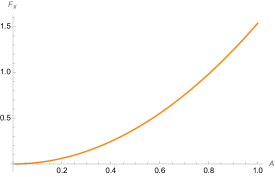
Figure 5: Fisher’s information measure for soliton in position space (mass distribution) in quartic potential.

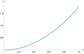
Figure 6: Fisher’s information measure for soliton in momentum space (mass distribution) in quartic potential.

Based on the findings, it is observed that there is a phenomenon of ”information propagation” of the solitonic mass distribution when it is exposed to the confining potential $V(x)=ax^{2}+bx^{4}$.

V Solitons in a Symmetric well

The prevalence of solitons is primarily attributed to a limited set of adaptable nonlinear equations that govern various physical and biological systems. Despite the distinct nature of these systems and their nonlinear characteristics, the mathematical equations describing them can exhibit significant similarities or even identical forms. Consequently, the study and analysis of these generic nonlinear models hold significant importance in diverse physical contexts, allowing for a deeper understanding of a wide range of phenomena. We shall consider ultra-fast pulsed fiber lasers as an example. It finds its application in the field of optical and quantum communication. One of the major factors that affect communication in this system is dispersion. Dispersion management is a key route for manipulating optical pulses for some desired output in ultra-fast optics. Minimal dispersion is achieved in the case of symmetric potential. So it’s crucial for us to understand its behavior in case of symmetric potential [39]. In this section, we shall discuss solitons in symmetric potential. We know the well-known symmetric potential as

$$V(x)=V_{0}\bigg{(}\frac{1-\lambda xcot(\lambda x)}{(\lambda x)^{2}}\bigg{)},$$ (46)

where, $V_{0}$ is a constant parameter, $\lambda$ corresponds to a parameter in the potential which has a unit of $[Length]^{-1}$.

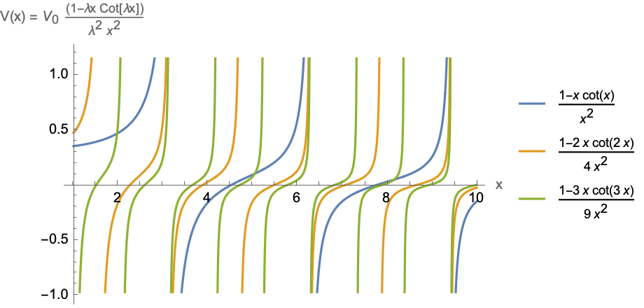
Figure 7: Symmetric potential for several values of parameter $\lambda$ and $V_{0}$ constant.

V.1 Constant mass

We start by calculating the wave function for this system for constant mass (i.e., $m=m_{0}$), Schrodinger equation for this system is simplified as follows

$$\frac{d^{2}\psi(x)}{dx^{2}}+\frac{2m_{0}}{\hbar^{2}}\Bigg{[}E-V_{0}\bigg{(}\frac{1-\lambda xcot(\lambda x)}{(\lambda x)^{2}}\bigg{)}\Bigg{]}\psi(x)=0,$$ (47)

The wave function is computed (briefly discussed in VII.2) and is given by

$$\psi(x)=\bigg{(}\frac{1}{\pi}\sqrt{\frac{2}{45}}\bigg{)}^{1/4}e^{\frac{-\lambda x^{2}}{2}}\bigg{[}1-0.087(4\lambda x^{2}-2)\bigg{]}.$$ (48)

In reciprocal space, the wave function $(\phi(k))$ can be written as

$$\phi(k)=\bigg{(}\frac{1}{\pi}\sqrt{\frac{2}{45}}\bigg{)}^{1/4}e^{\frac{-k^{2}}{2\lambda}}\bigg{[}\frac{1.174}{\sqrt{\lambda}}-\frac{0.348}{\lambda^{3/2}}(\lambda-k^{2})\bigg{]}.$$ (49)

V.1.1 Shannon Entropy

Shannon’s entropy in position space ($S_{x}$) is given by

$$S_{x}=-\int_{-\infty}^{\infty}|\psi(x)|^{2}\text{ln}|\psi(x)|^{2}dx,$$ (50)

and we obtain the form for Shannon entropy $(S_{x})$ as

$$S_{x}=-\int_{-\infty}^{\infty}\Bigg{(}\bigg{(}\frac{1}{\pi}\sqrt{\frac{2}{45}}\bigg{)}^{1/2}e^{-\lambda x^{2}}\bigg{[}1-0.087(4\lambda x^{2}-2)\bigg{]}^{2}\Bigg{)}\\ \Bigg{(}\frac{1}{2}\text{ln}\bigg{(}\frac{1}{\pi}\sqrt{\frac{2}{45}}\bigg{)}-\lambda x^{2}+2\text{ln}\bigg{[}1-0.087(4\lambda x^{2}-2)\bigg{]}\Bigg{)}dx,$$

Similarly, Shannon entropy in momentum space is given by

$$S_{k}=-\int_{-\infty}^{\infty}|\phi(k)|^{2}\text{ln}|\phi(k)|^{2}dx,$$ (51)

and we obtain the form for Shannon entropy $(S_{k})$ as

$$S_{k}=-\int_{-\infty}^{\infty}\bigg{(}\frac{1}{\pi}\sqrt{\frac{2}{45}}\bigg{)}^{1/2}e^{\frac{-k^{2}}{\lambda}}\bigg{[}\frac{1.174}{\sqrt{\lambda}}-\frac{0.348}{\lambda^{3/2}}(\lambda-k^{2})\bigg{]}^{2}\\ \Bigg{(}\frac{1}{2}\bigg{(}\frac{1}{\pi}\sqrt{\frac{2}{45}}\bigg{)}-\frac{k^{2}}{\lambda}+2\text{ln}\bigg{[}\frac{1.174}{\sqrt{\lambda}}-\frac{0.348}{\lambda^{3/2}}(\lambda-k^{2})\bigg{]}\Bigg{)}dk.$$

The numerical result of Shannon entropy for constant mass is presented in the following table:

$\lambda$	$S_{x}$	$S_{k}$	$S_{x}+S_{k}$	$1+\text{ln}\pi$
0.15	1.892	0.2565	2.149	2.1447
0.18	1.727	0.4434	2.170	2.1447
0.20	1.638	0.5353	2.174	2.1447
0.22	1.562	0.6903	2.252	2.1447
0.25	1.466	0.6960	2.162	2.1447
0.28	1.385	0.7619	2.147	2.1447
0.30	1.340	0.810	2.150	2.1447

Table 5: Numerical results of the Shannon entropy

V.1.2 Fisher’s Information measure

For an observable $x$, Fisher information ($F_{x}$) is given by

$$F_{x}=\int_{-\infty}^{\infty}|\psi(x)|^{2}\bigg{[}\frac{d}{dx}\text{ln}|\psi(x)|^{2}\bigg{]}^{2}dx>0,$$ (52)

and we obtain the form for Fisher information $(F_{x})$ as

$$F_{x}=\int_{-\infty}^{\infty}\Bigg{(}\bigg{(}\frac{1}{\pi}\sqrt{\frac{2}{45}}\bigg{)}^{1/2}e^{-\lambda x^{2}}\bigg{[}1-0.087(4\lambda x^{2}-2)\bigg{]}^{2}\\ \Bigg{[}-2\lambda x+\frac{1.392\lambda x}{1-0.087(4\lambda x^{2}-2)}\Bigg{]}^{2}\Bigg{)}dx.$$

In reciprocal space, Fisher information for an observable $k$, ($F_{k}$) is given by

$$F_{k}=\int_{-\infty}^{\infty}|\phi(k)|^{2}\bigg{[}\frac{d}{dk}\text{ln}|\phi(k)|^{2}\bigg{]}^{2}dk>0,$$ (53)

and we obtain the form for Fisher information $(F_{k})$ as

$$F_{k}=\int_{-\infty}^{\infty}\Bigg{(}\bigg{(}\frac{1}{\pi}\sqrt{\frac{2}{45}}\bigg{)}^{1/2}e^{\frac{-k^{2}}{\lambda}}\bigg{[}\frac{1.174}{\sqrt{\lambda}}-\frac{0.348}{\lambda^{3/2}}(\lambda-k^{2})\bigg{]}^{2}\\ \Bigg{[}\frac{-2k}{\lambda}+\frac{1.392}{\lambda^{3/2}(\frac{1.174}{\sqrt{\lambda}}-\frac{0.348}{\lambda^{3/2}}(\lambda-k^{2}))}\Bigg{]}^{2}\Bigg{)}dk.$$

We present the numerical result of Fisher’s information measure in the following table:

$\lambda$	$F_{x}$	$F_{k}$	$\sigma^{2}_{x}$	$\sigma^{2}_{k}$	$F_{x}\cdot F_{k}$
0.01	0.1834	557.04	139.26	0.0458	102.16
0.02	0.2595	196.94	49.235	0.0648	51.105
0.05	0.4103	49.823	12.455	0.1026	20.442
0.08	0.5190	24.618	6.154	0.1298	12.777
0.10	0.5803	17.615	4.403	0.1450	10.222
0.15	0.7107	9.588	2.397	0.1777	6.814
0.20	0.8206	6.228	1.557	0.2051	5.110
0.25	0.9175	4.456	1.114	0.2293	4.088

Table 6: Results for the uncertainty relation and Fisher information measure

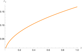
Figure 8: Fisher’s information measure for soliton in position space (constant mass) in symmetric well.

Figure 9: Fisher’s information measure for soliton in momentum space (constant mass) in symmetric well.

V.2 Mass distribution

For a mass distribution $m(x)=\frac{m_{0}}{1+x^{2}}$, Schrodinger equation is modified as follows

$$\frac{-\hbar^{2}}{2m}\frac{d^{2}\psi(x)}{dx^{2}}+\frac{-\hbar^{2}}{2}\frac{m^{\prime}(x)}{m(x)^{2}}\frac{d\psi(x)}{dx}+\Bigg{[}\frac{\hbar^{2}}{4}\frac{m^{\prime\prime}(x)}{m(x)^{2}}-\\ \frac{3\hbar^{2}}{8}\frac{m^{\prime}(x)^{2}}{m(x)^{3}}+V_{0}\bigg{(}\frac{1-\lambda xcot(\lambda x)}{(\lambda x)^{2}}\bigg{)}\Bigg{]}\psi(x)=E\psi(x).$$ (54)

We adopt stationary perturbation theory and variation principle to obtain the wave function [40]. Complete derivation of wave function is presented in Appendix (VII.2). We get the wave function as follows

$$\psi(x)\approx\frac{1}{\sqrt{\pi}}\frac{e^{\frac{-x^{2}}{2}}}{\sqrt{1+x^{2}}}\bigg{(}1-\frac{\lambda^{2}x^{2}}{10}+\frac{\lambda^{4}x^{4}}{126}-\frac{\lambda^{6}x^{6}}{2520}\bigg{)},$$ (55)

In momentum space, the wave function is obtained through fourier transforming the wave function in position space.

$$\phi(k)\approx\frac{1}{\sqrt{\pi}}\frac{e^{\frac{-k^{2}}{2}}}{\sqrt{1+\frac{k^{2}}{\lambda^{2}}}}\bigg{(}1+\frac{\lambda^{2}k^{2}}{10}+\frac{\lambda^{4}k^{4}}{126}+\frac{\lambda^{6}k^{6}}{2520}\bigg{)}.$$ (56)

V.2.1 Shannon entropy

Probability of finding the particle in the state $\psi(x,t)$ between the spatial interval $x$ and $x+dx$ describes as $|\psi(x,t)|^{2}\approx|\psi(x)|^{2}$. Shannon’s entropy in position space ($S_{x}$) is given by

$$S_{x}=-\int_{-\infty}^{\infty}|\psi(x)|^{2}\text{ln}|\psi(x)|^{2}dx,$$ (57)

and we obtain the form for Shannon entropy $(S_{x})$ as

$$S_{x}=-\int_{-\infty}^{\infty}\Bigg{(}\frac{1}{\pi}\frac{e^{-x^{2}}}{(1+x^{2})}\bigg{(}1-\frac{\lambda^{2}x^{2}}{10}+\frac{\lambda^{4}x^{4}}{126}-\frac{\lambda^{6}x^{6}}{2520}\bigg{)}^{2}\Bigg{)}\\ \Bigg{(}-\text{ln}\pi-x^{2}-\text{ln}(1+x^{2})+2\text{ln}\bigg{(}1-\frac{\lambda^{2}x^{2}}{10}+\frac{\lambda^{4}x^{4}}{126}-\frac{\lambda^{6}x^{6}}{2520}\bigg{)}\Bigg{)}dx.$$

In reciprocal space,

$$S_{k}=-\int_{-\infty}^{\infty}|\phi(k)|^{2}\text{ln}|\phi(k)|^{2}dk,$$ (58)

and we obtain the form for Shannon entropy $(S_{k})$ as

$$S_{k}=-\int_{-\infty}^{\infty}\frac{1}{\pi}\frac{e^{-k^{2}}}{(1+\frac{k^{2}}{\lambda^{2}})}\bigg{(}1+\frac{\lambda^{2}k^{2}}{10}+\frac{\lambda^{4}k^{4}}{126}+\frac{\lambda^{6}k^{6}}{2520}\bigg{)}^{2}\\ \Bigg{(}-\text{ln}\pi-k^{2}-\text{ln}(1+\frac{k^{2}}{\lambda^{2}})+2\text{ln}\bigg{(}1+\frac{\lambda^{2}k^{2}}{10}+\frac{\lambda^{4}k^{4}}{126}+\frac{\lambda^{6}k^{6}}{2520}\bigg{)}\Bigg{)}dk.$$

Finding an analytical solution for this particular equation will be complicated. So, we use some numerical techniques to find Shannon entropy for this system. The numerical result of Shannon entropy is presented in the following table:

$\lambda$	$S_{x}$	$S_{k}$	$S_{x}+S_{k}$	$1+\text{ln}\pi$
2.0	0.6033	1.6511	2.254	2.1447
2.1	0.6034	1.8394	2.443	2.1447
2.2	0.6107	2.0343	2.645	2.1447
2.3	0.6289	2.2036	2.832	2.1447
2.4	0.6630	2.2848	2.948	2.1447
2.5	0.7190	2.1661	2.885	2.1447
2.6	0.8035	1.6592	2.463	2.1447

Table 7: Numerical results of the Shannon entropy

V.2.2 Fisher’s Information measure

For an observable $x$, Fisher information ($F_{x}$) is given by

$$F_{x}=\int_{-\infty}^{\infty}|\psi(x)|^{2}\bigg{[}\frac{d}{dx}\text{ln}|\psi(x)|^{2}\bigg{]}^{2}dx>0,$$ (59)

and we obtain the form for Fisher’s information $(F_{x})$ as

$$F_{x}=\int_{-\infty}^{\infty}\Bigg{(}\frac{1}{\pi}\frac{e^{-x^{2}}}{(1+x^{2})}\bigg{(}1-\frac{\lambda^{2}x^{2}}{10}+\frac{\lambda^{4}x^{4}}{126}-\frac{\lambda^{6}x^{6}}{2520}\bigg{)}^{2}\Bigg{)}\\ \Bigg{[}\frac{d}{dx}\Bigg{(}-\text{ln}\pi-x^{2}-\text{ln}(1+x^{2})+2\text{ln}\bigg{(}1-\frac{\lambda^{2}x^{2}}{10}+\frac{\lambda^{4}x^{4}}{126}-\frac{\lambda^{6}x^{6}}{2520}\bigg{)}\Bigg{)}\Bigg{]}^{2}dx.$$

In reciprocal space, Fisher information for an observable $k$, ($F_{k}$) is given by

$$F_{k}=\int_{-\infty}^{\infty}|\phi(k)|^{2}\bigg{[}\frac{d}{dk}\text{ln}|\phi(k)|^{2}\bigg{]}^{2}dk>0.$$ (60)

and we obtain the form for Fisher’s information $(F_{k})$ as

$$F_{k}=\int_{-\infty}^{\infty}\frac{1}{\pi}\frac{e^{-k^{2}}}{(1+\frac{k^{2}}{\lambda^{2}})}\bigg{(}1+\frac{\lambda^{2}k^{2}}{10}+\frac{\lambda^{4}k^{4}}{126}+\frac{\lambda^{6}k^{6}}{2520}\bigg{)}^{2}\\ \Bigg{[}\frac{d}{dk}\Bigg{(}-\text{ln}\pi-k^{2}-\text{ln}(1+\frac{k^{2}}{\lambda^{2}})+2\text{ln}\bigg{(}1+\frac{\lambda^{2}k^{2}}{10}+\frac{\lambda^{4}k^{4}}{126}+\\ \frac{\lambda^{6}k^{6}}{2520}\bigg{)}\Bigg{)}\Bigg{]}^{2}dk.$$

$\lambda$	$F_{x}$	$F_{k}$	$\sigma^{2}_{x}$	$\sigma^{2}_{k}$	$F_{x}\cdot F_{k}$
0.01	1.3600	50.009	12.502	0.34	68.012
0.02	1.3595	25.0406	6.260	0.3398	34.042
0.03	1.3596	16.7331	4.183	0.1942	22.750
0.04	1.3597	12.5902	3.1476	0.3399	17.119
0.05	1.3597	10.1128	2.5282	0.3399	13.750
0.08	1.36003	6.4257	1.6064	0.3400	8.739
0.1	1.3606	5.2142	1.3036	0.3402	7.094

Table 8: Results for the uncertainty relation and Fisher information measure

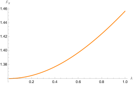
Figure 10: Fisher’s information measure for soliton in position space (mass distribution) in symmetric well.

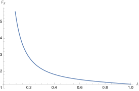
Figure 11: Fisher’s information measure for soliton in momentum space (mass distribution) in symmetric well.

Based on the findings, it is observed that there is a phenomenon of ”information propagation” in the solitonic mass distribution when it is exposed to the confining potential $V(x)=V_{0}\bigg{(}\frac{1-\lambda xcot(\lambda x)}{(\lambda x)^{2}}\bigg{)}$.

VI Summary and Remarks

This study focused on examining Shannon entropy and Fisher information concerning a constant mass and solitonic mass distribution. The work explored the solutions of the stationary Schrodinger equation, where the mass depends on the position and is exposed to a quartic ($ax^{2}+bx^{4}$) and symmetric potential ($V_{0}\bigg{(}\frac{1-\lambda xcot(\lambda x)}{(\lambda x)^{2}}\bigg{)}$). After obtaining the analytical solutions of the model, the investigation proceeded to study the Shannon entropy and Fisher’s information associated with the ground state energy levels. The observations indicate that the solitonic mass distribution under the quartic potential exhibits higher Shannon entropy values compared to the case with a constant mass. Hence, the combined value of Shannon entropy (i.e., the sum of $S_{x}$ and $S_{k}$) is greater for the solitonic mass distribution than for a constant mass scenario. On the other hand, the Fisher information is higher for the solitonic mass distribution in comparison to the constant mass scenario. In the context of information [41] and communication theories [42], based on our observations, we can deduce that the solitonic system with mass distribution possesses attributes that empower it to manage unpredictability, convey abundant information, demonstrate heightened responsiveness, and function effectively in various communication and data processing scenarios. Moreover, this system also displays greater capacity, resilience, and versatility, leading to enhanced performance and reliability in contemporary communication situations than the system with a constant mass. Thus for effective communication, a solitonic mass distribution can be preferred.

When considering solitons in symmetric potential, we notice distinct behavior compared to that in quartic potential. The results show that the solitonic mass distribution within the symmetric well has greater Shannon entropy values compared to a constant mass scenario. As a consequence, the combined Shannon entropy (the sum of $S_{x}$ and $S_{k}$) is greater for the solitonic mass distribution than the constant mass scenario. On the contrary, the Fisher information is higher for constant mass in contrast to mass distribution. In information theory [41], a solitonic system with constant mass distribution reflects a system with increased unpredictability, richer information content, and heightened sensitivity to changes. This combination leads to a greater capacity for data transmission, improved parameter estimation, and enhanced performance in communication and data processing. The system can efficiently handle diverse information and is more robust against noise and disturbances, making it well-suited for various applications in information theory and communication. However, managing the higher complexity and resource requirements of such a system may be necessary. Nonetheless, in communication systems [42], employing a solitonic system with constant mass leads to greater capacity, improved noise resilience, and enhanced data transmission capabilities, making them well-suited for modern communication scenarios and emerging technologies. Therefore, based on our observations, we can infer that an improved quantum communication can be attained using two types of solitonic systems: one under a symmetric well with constant mass, and the other under a quartic potential with a mass distribution.

In conclusion, the extension of the current work to investigate Shannon and Fisher’s information measure in the context of Sine-Gordon solitons and solitons in Bose-Einstein condensates (BEC) within the Gross-Pitaevskii equation (GPE) framework will provide a deeper and more comprehensive understanding of the underlying complexities of these intriguing systems. The exploration of information entropy, both from a Shannon and Fisher perspective, will unveil valuable insights into the intrinsic nature of solitonic phenomena. By quantifying the uncertainty and information content associated with these soliton structures, we gain a quantitative measure of the intricate balance between coherence, localization, and the underlying dynamics of the systems under consideration. Studying information entropy in Sine-Gordon solitons will not only elucidate the richness of these topologically nontrivial solutions but will also establish a connection between information theory and field theory [43]. The quantification of information entropy in this context will shed light on the interplay between spatial distribution, energy concentration, and the stability of solitonic configurations. Such insights not only will enhance our theoretical understanding but also paves the way for potential applications in fields such as data encoding, signal processing, and quantum information. Extending the analysis to solitons in BEC gases governed by the GPE will introduce a quantum mechanical dimension to the study. The intricate balance between quantum coherence and nonlinear interactions inherent in BEC systems will add a layer of complexity to the information entropy analysis. The quantification of information content in these systems will offer a unique perspective on the emergence and behavior of solitons in a quantum context, contributing to the broader understanding of quantum coherence and correlations. The culmination of this work will highlight the universality of information entropy as a powerful tool for characterizing and comparing soliton dynamics across different physical systems.

VII Appendix

VII.1 Solitons in Quartic potential - Wave function computation

VII.1.1 Constant mass

Our aim is to solve eq.(19). We employ the technique by assuming the solution of this particular differential equation, viz, Gaussian wave function. Previously, this assumption is used only to solve the system’s quadratic potentials with time dependence. However, in [44], it is shown that the same method also works in the case of quartic potential. The main difference is that all the systems which are studied using this formulation work only for time-dependent cases, but we work with solitonic systems which are time-independent. This formulation (assumption) works even in our case. The Gaussian function is assumed to have some parameters $r,s,q$ and a normalization factor of $N$. We assume the solution $\psi(x)$ as

$$\psi(x)=N\text{exp}\bigg{[}rx^{2}+sx+q\bigg{]}.$$ (61)

Substituting this assumption in this differential equation eq. (19) we get

$$\frac{d^{2}\psi}{dx^{2}}=(2rx+s)^{2}\psi(x)+2r\psi(x),$$

Thus we get,

$$(2rx+s)^{2}\psi(x)+2r=Cx^{4}+Bx^{2}-A,$$

By comparing the co-coefficients, we get the wave function of this particular system to be

$$\psi(x)=N\text{exp}\bigg{[}\frac{-A}{2}x^{2}\bigg{]},$$ (62)

Upon normalising we get the final wave equation to be

$$\psi(x)=\sqrt{\frac{A}{\pi}}\text{exp}\bigg{[}\frac{-A}{2}x^{2}\bigg{]}.$$ (63)

VII.1.2 Mass distribution

The Schrodinger equation for the given mass distribution is given by,

$$\frac{-\hbar^{2}}{2m_{0}}(1+x^{2})\frac{d^{2}\psi}{dx^{2}}+x^{2}\psi+x^{4}\psi=E\psi,$$ (64)

$$\frac{d^{2}\psi}{dx^{2}}-\frac{2m_{0}}{\hbar^{2}}x^{2}\psi=\frac{-2m_{0}E}{\hbar^{2}}\frac{1}{1+x^{2}}\psi,$$

$$\frac{d^{2}\psi}{dx^{2}}+\frac{2m_{0}}{\hbar^{2}}\bigg{(}\frac{E}{1+x^{2}}-x^{2}\bigg{)}\psi=0.$$

We find the solution analytically by Perturbation theory, total Hamiltonian is given by $H=H_{0}+H_{1}$. The corresponding potential for $H_{0}$ is $V_{0}$ which is equal to $x^{2}$ and $H_{1}=\lambda x^{4}$ (perturbation term), where $\lambda$ is small. The wave function corresponding to $H_{0}$ (zeroth order perturbation theory) is

$$\psi_{0}(x)=A\text{exp}\bigg{[}\frac{-x^{2}}{2(1+x^{2})}\bigg{]}H_{n}(x),$$ (65)

where, $H_{n}$ is the Hermite polynomial for a given state $n$, $A$ is the normalization constant. However, we are interested in computing the wave function only for the ground state (i.e. $n=0$). Therefore, we get the Hermite polynomial to be, $H_{0}=1$. Therefore, the wave function for the system in the ground state is given by

$$\psi_{0}(x)=A\text{exp}\bigg{[}\frac{-x^{2}}{2(1+x^{2})}\bigg{]},$$ (66)

here, $\lambda x^{4}$ term is looked as a perturbation to the $x^{2}$ term. Thus the wave function perturbed to the first order is given by

$$\psi_{1}(x)=\sum_{n}\frac{\bra{n}H_{1}\ket{0}}{E_{0}-E_{n}}\psi_{0}(x),$$ (67)

For ground state, we get the perturbed wave function ($\psi_{1}(x)$) as

$$\psi(x)=\frac{A}{(1+x^{2})^{1/4}}\text{exp}\bigg{[}\frac{-x^{2}}{2(1+x^{2})}\bigg{]}.$$ (68)

VII.2 Solitons in Symmetric well - Wave function computation

VII.2.1 Constant mass

For a constant mass, the Schrodinger equation for symmetric potential is given by

$$\frac{d^{2}\psi(x)}{dx^{2}}+\frac{2m_{0}}{\hbar^{2}}\Bigg{[}E-V_{0}\bigg{(}\frac{1-\lambda xcot(\lambda x)}{(\lambda x)^{2}}\bigg{)}\Bigg{]}\psi(x)=0,$$ (69)

We find the solution analytically by Perturbation theory, total Hamiltonian is given by $H=H_{0}+H_{1}$. The corresponding potential for $H_{0}$ is $V_{0}$ which is equal to the potential of the harmonic oscillator. We use stationary perturbation theory to obtain the wave function and energy levels for this particular system. This potential (up to $\mathcal{O}(x^{6})$ term) is expressed as

$$V(x)\approx V_{0}\bigg{(}\frac{1}{3}+\frac{1}{45}(\lambda x)^{2}+\frac{2}{945}(\lambda x)^{4}+\frac{1}{4725}(\lambda x)^{6}\bigg{)}.$$

The unperturbed hamiltonian is $H_{0}=\frac{V_{0}}{45}(\lambda x)^{2}$ and the perturbed hamiltonian ($H_{1}$) is given by,

$$H_{1}(x)=V_{0}\bigg{(}\frac{1}{3}+\frac{2}{945}(kx)^{4}+\frac{1}{4725}(kx)^{6}\bigg{)}$$ (70)

The wave function of solitons in first-order perturbation theory is given by

$$\psi^{(0)}_{n}(u)=\bigg{(}\frac{\lambda}{\pi}\bigg{)}^{1/4}\frac{1}{\sqrt{2^{n}}n!}H_{n}(u)e^{\frac{-u^{2}}{2}},$$ (71)

where, $u=\sqrt{\lambda}x$ and $H_{n}$ is the Hermite polynomial and the values are as follows:

$$H_{0}=1$$

$$H_{1}=2u$$

$$H_{2}=4u^{2}-2$$

$$H_{3}=8u^{3}-12u$$

$$H_{4}=16u^{4}-48u^{2}+12$$

For ground states ($n=0$), we get the wave function $(\psi^{(0)}_{0})$ to be

$$\psi^{(0)}_{0}(x)=\bigg{(}\frac{\lambda}{\pi}\sqrt{\frac{2}{45}}\bigg{)}^{1/4}\text{exp}\bigg{[}-\lambda\frac{x^{2}}{2}\bigg{]}.$$ (72)

Eigen value for unperturbed system reads $E^{(0)}_{0}=\frac{1}{2}$.

$$\psi^{(0)}_{1}(x)=\psi^{(0)}_{0}+\frac{\bra{\psi^{(0)}_{2}}H_{1}(x^{4})\ket{\psi^{(0)}_{0}}}{E^{(0)}_{0}-E^{(2)}_{0}}\psi_{2}^{(0)}+\frac{\bra{\psi^{(0)}_{4}}H_{1}(x^{4})\ket{\psi^{(0)}_{0}}}{E^{(0)}_{0}-E^{(0)}_{4}}\psi_{4}^{(0)}.$$ (73)

$$\psi^{(0)}_{1}(x)=\psi^{(0)}_{0}+\frac{\bra{2}H_{1}(x^{4})\ket{0}}{E^{(0)}_{0}-E^{(2)}_{0}}\psi_{2}^{(0)}+\frac{\bra{4}H_{1}(x^{2})\ket{0}}{E^{(0)}_{0}-E^{(0)}_{4}}\psi_{4}^{(0)}$$

We only look into unperturbed and the second order state. Thus we get the wave function as follows

$$\psi(x)=\psi^{(0)}_{0}+\frac{\bra{2}H_{1}\ket{0}}{E^{(0)}_{0}-E^{(2)}_{0}}.$$ (74)

Therefore we get the final wave function as,

$$\psi(u)=\bigg{(}\frac{1}{\pi}\sqrt{\frac{2}{45}}\bigg{)}^{1/4}e^{\frac{-u^{2}}{2}}\bigg{[}1-0.087(4u^{2}-2)\bigg{]},$$ (75)

where, $u=\sqrt{\lambda}x$. We write the final expression as follows

$$\psi(x)=\bigg{(}\frac{1}{\pi}\sqrt{\frac{2}{45}}\bigg{)}^{1/4}e^{\frac{-\lambda x^{2}}{2}}\bigg{[}1-0.087(4\lambda x^{2}-2)\bigg{]}.$$ (76)

VII.2.2 Mass distribution

The potential of symmetric well is given by

$$V(x)=V_{0}\bigg{(}\frac{1-\lambda xcot(\lambda x)}{(\lambda x)^{2}}\bigg{)},$$ (77)

For the sake of simplicity, we consider the value of $V_{0}$ to be $1$. This potential can be expressed as,

$$V(x)=-4\sum^{\infty}_{n=1}\frac{(-1)^{n}(2\lambda x)^{2n-2}}{(2n!)}B_{2n},\hskip 15.00002pt\forall\lambda x<\pi.$$ (78)

The first few terms are given by,

$$\sum^{\infty}_{n=1}\frac{(-1)^{n}(2\lambda x)^{2n-2}}{(2n!)}B_{2n}=\frac{-B_{2}}{2}+\frac{B_{4}}{6}(\lambda x)^{2}-\cdots$$ (79)

We use stationary perturbation theory to obtain the wave function and energy levels for this particular system. This potential (up to $\mathcal{O}(x^{6})$ term) is expressed as

$$V(x)=\frac{1}{3}+\frac{1}{45}(\lambda x)^{2}+\frac{2}{945}(\lambda x)^{4}+\frac{1}{4725}(\lambda x)^{6}.$$ (80)

The Schrodinger equation for the given mass distribution, $m(x)=\frac{1}{1+x^{2}}$ (assuming the value of $m_{0}$ to be $1$), we get

$$\frac{d^{2}\psi(x)}{dx^{2}}+\frac{2}{\hbar^{2}}\Bigg{[}E-V_{0}\bigg{(}\frac{1-\lambda xcot(\lambda x)}{(\lambda x)^{2}}\bigg{)}\Bigg{]}\bigg{(}\frac{1}{1+x^{2}}\bigg{)}\psi(x)=0,$$ (81)

We work with perturbation theory for small values of $\lambda$ and the usual convention $\hbar=1=V_{0}$. Thus we get

$$\frac{d^{2}\psi(x)}{dx^{2}}+2\Bigg{[}E-\bigg{(}\frac{1}{3}+\frac{1}{45}(\lambda x)^{2}+\frac{2}{945}(\lambda x)^{4}+\frac{1}{4725}(\lambda x)^{6}\bigg{)}\Bigg{]}\\ \bigg{(}\frac{1}{1+x^{2}}\bigg{)}\psi(x)=0,$$ (82)

The first-order correction to the wave function $\psi(x)$ can be calculated using the first-order perturbation theory formula

$$\psi_{1}(x)=\sum_{n\neq 0}\frac{\bra{\psi^{(0)}_{n}}H_{1}\ket{\psi^{(0)}_{0}}}{E^{0}_{0}-E^{0}_{n}}\psi_{0}(x),$$ (83)

where, $H_{1}$ is the perturbation term. In our case, it’s our usual potential. Now, the first-order perturbation correction to the final ground state wave function is,

$$\psi(x)\approx\frac{1}{\sqrt{\pi}}\frac{e^{\frac{-x^{2}}{2}}}{\sqrt{1+x^{2}}}\bigg{(}1-\frac{\lambda^{2}x^{2}}{10}+\frac{\lambda^{4}x^{4}}{126}-\frac{\lambda^{6}x^{6}}{2520}\bigg{)}.$$ (84)

References

- [1] P. G. Drazin, R. S. Johnson, Solitons: an introduction, Vol. 2, Cambridge university press, 1989.
- [2] V. Rubakov, Classical theory of gauge fields, Princeton University Press, 2009.
- [3] J. Preskill, Quantum computing 40 years later, arXiv preprint arXiv:2106.10522 (2021).
- [4] P. Drummond, R. Shelby, S. Friberg, Y. Yamamoto, Quantum solitons in optical fibres, Nature 365 (6444) (1993) 307–313.
- [5] H. A. Haus, W. S. Wong, Solitons in optical communications, Reviews of modern physics 68 (2) (1996) 423.
- [6] I. Abram, Quantum solitons, Physics world 12 (2) (1999) 21.
- [7] R. Rajaraman, Solitons and instantons, 1982.
- [8] W.-P. Su, J. R. Schrieffer, A. J. Heeger, Solitons in polyacetylene, Physical review letters 42 (25) (1979) 1698.
- [9] M. Planck, Treatise on thermodynamics, Courier Corporation, 2013.
- [10] P. Busch, T. Heinonen, P. Lahti, Heisenberg’s uncertainty principle, Physics reports 452 (6) (2007) 155–176.
- [11] P. Busch, T. Heinonen, P. Lahti, Heisenberg’s uncertainty principle, Physics reports 452 (6) (2007) 155–176.
- [12] A. Orłowski, Information entropy and squeezing of quantum fluctuations, Physical Review A 56 (4) (1997) 2545.
- [13] R. Atre, A. Kumar, N. Kumar, P. K. Panigrahi, Quantum-information entropies of the eigenstates and the coherent state of the pöschl-teller potential, Physical Review A 69 (5) (2004) 052107.
- [14] E. Romera, F. de Los Santos, Identifying wave-packet fractional revivals by means of information entropy, Physical review letters 99 (26) (2007) 263601.
- [15] A. Galindo, P. Pascual, Quantum mechanics I, Springer Science & Business Media, 2012.
- [16] M. Stein, A. Mezghani, J. A. Nossek, A lower bound for the fisher information measure, IEEE Signal Processing Letters 21 (7) (2014) 796–799.
- [17] S. Watanabe, Algebraic geometrical method in singular statistical estimation, in: Quantum Bio-Informatics: From Quantum Information to Bio-Informatics, World Scientific, 2008, pp. 325–336.
- [18] J. M. Bernardo, A. F. Smith, Bayesian theory, Vol. 405, John Wiley & Sons, 2009.
- [19] R. A. Fisher, Theory of statistical estimation, in: Mathematical proceedings of the Cambridge philosophical society, Vol. 22, Cambridge University Press, 1925, pp. 700–725.
- [20] C. A. Fuchs, A. Peres, Quantum-state disturbance versus information gain: Uncertainty relations for quantum information, Physical Review A 53 (4) (1996) 2038.
- [21] W. Ochs, Basic properties of the generalized boltzmann-gibbs-shannon entropy, Reports on Mathematical Physics 9 (2) (1976) 135–155.
- [22] W. Beckner, Inequalities in fourier analysis, Annals of Mathematics 102 (1) (1975) 159–182.
- [23] I. Bialynicki-Birula, J. Mycielski, Commun. math. phys. (1975).
- [24] V. Majernik, T. Opatrnỳ, Entropic uncertainty relations for a quantum oscillator, Journal of Physics A: Mathematical and General 29 (9) (1996) 2187.
- [25] M. W. Coffey, Semiclassical position and momentum information entropy for sech2 and a family of rational potentials, Canadian Journal of Physics 85 (7) (2007) 733–743.
- [26] E. Aydiner, C. Orta, R. Sever, Quantum information entropies of the eigenstates of the morse potential, International Journal of Modern Physics B 22 (03) (2008) 231–237.
- [27] J. S. Dehesa, W. Van Assche, R. J. Yáñez, Information entropy of classical orthogonal polynomials and their application to the harmonic oscillator and coulomb potentials, Methods and Applications of Analysis 4 (1) (1997) 91–110.
- [28] J. Rifkin, Entropy: a new world view.[social and political implications of the second law of thermodynamics] (1980).
- [29] E. H. Lieb, J. Yngvason, The physics and mathematics of the second law of thermodynamics, Physics Reports 310 (1) (1999) 1–96.
- [30] R. A. Fisher, On the mathematical foundations of theoretical statistics, Philosophical transactions of the Royal Society of London. Series A, containing papers of a mathematical or physical character 222 (594-604) (1922) 309–368.
- [31] Q.-G. Zhu, H. Kroemer, Interface connection rules for effective-mass wave functions at an abrupt heterojunction between two different semiconductors, Physical Review B 27 (6) (1983) 3519.
- [32] R. Shankar, Principles of quantum mechanics, Springer Science & Business Media, 2012.
- [33] V. I. Kruglov, H. Triki, Coupled multi-quartic and multi-dipole solitons in highly dispersive optical fibers, arXiv preprint arXiv:2301.02351 (2023).
- [34] A. Höök, M. Karlsson, Ultrashort solitons at the minimum-dispersion wavelength: effects of fourth-order dispersion, Optics letters 18 (17) (1993) 1388–1390.
- [35] M. Karlsson, A. Höök, Soliton-like pulses governed by fourth order dispersion in optical fibers, Optics communications 104 (4-6) (1994) 303–307.
- [36] S. Roy, F. Biancalana, Formation of quartic solitons and a localized continuum in silicon-based slot waveguides, Physical Review A 87 (2) (2013) 025801.
- [37] V. I. Kruglov, J. D. Harvey, Solitary waves in optical fibers governed by higher-order dispersion, Physical Review A 98 (6) (2018) 063811.
- [38] Q.-G. Zhu, H. Kroemer, Interface connection rules for effective-mass wave functions at an abrupt heterojunction between two different semiconductors, Physical Review B 27 (6) (1983) 3519.
- [39] S. K. Turitsyn, B. G. Bale, M. P. Fedoruk, Dispersion-managed solitons in fibre systems and lasers, Physics reports 521 (4) (2012) 135–203.
- [40] L. B. d. Carvalho, W. C. d. Santos, E. d. A. Correa, Solution of the 1d schrödinger equation for a symmetric well, Revista Brasileira de Ensino de Física 41 (2019).
- [41] R. M. Gray, Entropy and information theory, Springer Science & Business Media, 2011.
- [42] D. Shaw, C. H. Davis, Entropy and information: A multidisciplinary overview, Journal of the American Society for Information Science 34 (1) (1983) 67–74.
- [43] R. Radhakrishnan, V. K. Ojha, Wigner distribution of sine-gordon and kink solitons, Modern Physics Letters A 37 (37n38) (2022) 2250236.
- [44] S. Deffner, Nonlinear speed-ups in ultracold quantum gases, Europhysics Letters 140 (4) (2022) 48001.