[CII] Emission in a Self-Regulated Interstellar Medium

Abstract

The [CII] 157.74 $\mu$m fine structure transition is one of the brightest and most well-studied emission lines in the far-infrared (FIR), produced in the interstellar medium (ISM) of galaxies. We study its properties in sub-pc resolution hydrodynamical simulations for an ISM patch with gas surface density of $\Sigma_{\rm{g}}=10\;M_{\odot}\;\rm{pc}^{-2}$, coupled with time-dependent chemistry, far-ultraviolet (FUV) dust and gas shielding, star formation, photoionization and supernova (SN) feedback, and full line-radiative transfer. The [CII] 157.74 $\mu$m line intensity correlates with star formation rate (SFR), and scales linearly with metallicity, and is, therefore, a good SFR tracer even in metal-poor environments, where molecular lines might be undetectable. We find a [CII]-to-H₂ conversion factor that is well described by the power law $X_{\rm{[CII]}}=6.31\times 10^{19}\;Z^{\prime\;0.17}\;(\rm{cm}^{-2}\;(\rm{K}\;\rm{km}\;\rm{s}^{-1})^{-1})$. Our results are in agreement with galaxy surveys in all but the lowest metallicity run. We find that resolving the clumpy structure of the dense interstellar medium (ISM) is important as it dominates [CII] 157.74 $\mu$m emission. We compare our full radiative transfer computation with the optically-thin limit, and find that [CII] emission only begins approaching the optically thick limit at super-solar metallicity, for our assumed gas surface density.

1. Introduction

Singly ionized carbon (C⁺) is an important component of the interstellar medium (ISM). Given its low ionization potential of 11.26 eV, it is abundant in the warm- and cold neutral ISM (WNM, CNM), as well as part of the molecular ISM, as the carbon is ionized by far-ultraviolet (FUV) radiation longward of the Lyman limit which escapes regions of ionized gas surrounding hot OB stars. It also resides in HII regions alongside higher ionization stages of carbon. C⁺ is an important coolant in the cold ISM, via fine structure line emission at 157.74 $\mu$m (hereafter [CII] emission; Field et al., 1969; Draine, 1978; Crawford et al., 1985; Bialy & Sternberg, 2019). [CII] is the strongest spectral line in the far-infrared in most galaxies. It radiates away energy injected into the neutral atomic components of the ISM, mostly by FUV dust photo-electric heating. The upper level of the transition is excited by collisions, mostly with neutral and molecular hydrogen in the neutral ISM, and with electrons in HII regions. At sufficient densities, [CII] emission allows gas to cool down to temperatures of $\sim$10² K, owing to its low excitation threshold of 91.21 K (Dalgarno & McCray, 1972). [CII] emission is thus important for the thermodynamics of star formation, as it requires that gas cools and collapses under its self-gravity. [CII] emission is therefore ubiquitous in observations of stellar nurseries in our galaxy, as well as tracing star formation in extragalactic sources.

In recent decades, observations of [CII] emission have been pushed to higher redshifts, reaching as high as $z\sim 7$, mainly due to the operation of large millimeter wave interferometers such as the Atacama Large Millimeter/submillimeter Array (ALMA) and the Northern Extended Millimeter Array (NOEMA). Observations have established a correlation between star formation rate (SFR) and [CII] line luminosity. At redshifts $z\approx 0$ the Infrared Space Observatory (De Looze et al., 2011) and the Herschel Space Observatory (De Looze et al., 2014; Herrera-Camus et al., 2015) first established the [CII]-SFR relation on both galactic scales as well as on a spatially resolved level. On galactic scales, this relationship seems to hold for higher redshift systems as well, as revealed by ALMA up to $z\sim 7$ (Le Fèvre et al., 2020; Schaerer et al., 2020; Bouwens et al., 2022; Harikane et al., 2020).

Most of the cold gas mass in the ISM is in the form of H₂, but due to its lack of permanent dipole moment, it does not radiate efficiently at the low ($T\lesssim 10^{2}$ K) temperatures (Parmar et al., 1991; Richter et al., 1995) of the cold ISM. [CII], alongside other emission lines (especially CO rotational emission), is therefore one of the main tracers of cold gas in galaxies. In cold dense gas that is shielded from FUV radiation, C⁺ can recombine efficiently to form C, which in turn forms CO in even more shielded regions of gas clouds (Tielens & Hollenbach, 1985; Sternberg & Dalgarno, 1995; Wolfire et al., 2022). At the same time, dense HII regions, which have a significant fraction of their mass in C⁺, also show strong [CII] emission. This adds a layer of complexity of tracing cold gas and star formation using the [CII] line, as the origin of the radiation needs to be understood to properly interpret observational data.

Traditionally, CO line emission is used to trace cold molecular gas. Specifically, the intensity of the CO $J=1-0$ line at 2.6 mm can be measured, and converted into H₂ column density using the CO-to-H₂ conversion factor defined by

$$X_{\rm{CO}}\equiv\frac{N_{\rm{H}_{2}}}{W_{\rm{CO}}},$$ (1)

where $N_{\rm{H}_{2}}$ is the H₂ column density, and $W_{\rm{CO}}$ is the velocity integrated brightness temperature of the CO $J=1-0$ line. One can similarly define a [CII]-to-H₂ conversion factor

$$X_{\rm{[CII]}}\equiv\frac{N_{\rm{H}_{2}}}{W_{\rm{[CII]}}},$$ (2)

where $W_{\rm{[CII]}}$ is the velocity integrated brightness temperature of the [CII] line. The potential and applicability of such a conversion factor ties into the question of the ”CO-dark” H₂, i.e., molecular gas not traced by CO emission. CO-dark molecular gas is a result of the HI-to-H₂ transition taking place at lower column densities than the C⁺-C-CO transition, and the fraction of H₂ in this intermediate layer varies with gas properties, most importantly with gas metallicity, as the CO core becomes smaller and might even be absent entirely (Wolfire et al., 2010; Hu et al., 2022). This question has been investigated observationally (Langer et al., 2010, 2014; Pineda et al., 2013), as well as using 1D photodissociation region (PDR) models (Tielens & Hollenbach, 1985; Pak et al., 1998; Hollenbach & Tielens, 1999; Wolfire et al., 2022). Madden et al. (2020) used PDR modelling to analyze observations from the Dwarf Galaxy Survey (Madden et al., 2013), and found a relation between H₂ mass and [CII] line luminosity of the form $M_{\rm{H}_{2}}=10^{2.12}\times(L_{\rm{[CII]}}/L_{\odot})^{0.97}M_{\odot}$, which for their model geometry corresponds to $X_{\rm{[CII]}}\approx 1.4\times 10^{20}$ cm^-2 $(\rm{K\;km\;s}^{-1})^{-1}$, comparable to the Milky Way value of $X_{\rm{CO}}=2\times 10^{20}$ cm^-2 (K km s^-1)^-1 (Bolatto et al., 2013).

Indeed, theoretical models of 1-dimensional photodissociation regions (PDRs) can be used to quantitatively model the connection between gas properties and [CII] emission. In recent years, however, the study of the ISM emission in 3D hydrodynamical numerical simulations has been made possible thanks to the advent of large supercomputers. Simulations can now track gas dynamics, thermal state, chemistry (albeit usually in post-processing), and the different star formation feedback mechanisms, to give a more realistic context to the theoretical study of ISM properties. Hydrodynamical simulations have attempted to capture different spatial scales, from single cloud, through galactic, to cosmological scales.

In order to capture the cold gas component of the ISM in a realistic environment, however, one must spatially resolve the scale of dense molecular cores, as well as have the spatial and temporal extent that captures the larger WNM gas reservoir and the effects of stellar feedback due to photoionization and supernovae (SNe). The emerging life cycle of the ISM includes the cooling and gravitational collapse of gas clouds to form stars, followed by heating, ionization, dispersal, and injection of turbulence into the gas by massive stars and SNe. Simulations of [CII] emission vary in scale, hydrodynamical setup, implementation of sub-grid physical models, and treatment of radiative transfer. Hu et al. (2019) carried out a simulation of an isolated dwarf galaxy at high spatial resolution, computing unresolved [CII] emission under the optically thin assumption. Lupi & Bovino (2020) simulated a dwarf galaxy using the zoom-in technique, where the boundary conditions of gas flow are determined by a larger, lower resolution cosmological simulation, and again calculated the unresolved, optically thin, [CII] emission. Bisbas et al. (2022) simulated the merger of two dwarf galaxies, and post processed their simulation results with a full radiative transfer computation. Another method used is post processing each particle in the simulation using tabulated CLOUDY photoionization models (Ferland et al., 2017). This technique has been implemented by Liang et al. (2023) in both zoom-in and high resolution cosmological simulations, Olsen et al. (2017) in a zoom-in simulation, and Katz et al. (2022) in a cosmological simulation. While these simulations cover large volumes at varying spatial resolution, they do not resolve the clumpy structure of the dense ISM, nor do they provide a systematic study of the effect of metallicity. Franeck et al. (2018); Ebagezio et al. (2022) used an analogue of the zoom-in technique but zooming in on a single cloud within a simulation of a patch of a galactic disk. Their simulations have very high spatial resolution, include non-equilibrium chemistry and cooling, and they post-process their results using photoionization modelling in order to account for stellar photoionization feedback. They also perform full radiative transfer calculations in order to obtain synthetic [CII] emission maps. Their high resolution means that they simulate a relatively small volume, for a simulation time shorter than the typical lifespan of a gas cloud, and for solar metallicity. They quantified $X_{\rm{[CII]}}$ for each collapsing molecular cloud, and found values ranging from $\sim 0.5$ to $\sim 8\times$10²⁰ cm^-2 (K km s^-1)^-1. The range in values of $X_{\rm{[CII]}}$ is due to both time variation and variation between clouds and simulation setup.

While most simulations investigating the [CII]-SFR relation succeed in reproducing observations, albeit to different levels of success, they usually use either a constant metallicity or couple the metallicity evolution to the SFR in the galaxy. Lagache et al. (2018) used a semi-analytic approach to model the [CII]-SFR relation, and found a wide correlation between [CII] luminosity and metallicity, with a very large scatter of $~{}0.8$ dex. Vallini et al. (2015) varied the metallicity in a single snapshot of a zoom-in cosmological simulation, and found a positive trend in the [CII] luminosity-SFR ratio with metallicity. Olsen et al. (2015) found a weaker trend in the [CII] luminosity-SFR ratio with metallicity, but did not rule it out, as their results spanned a range of just over 0.5 dex in carbon metallicity.

Hu et al. (2021) (hereafter HSvD21) performed high-resolution simulations of a SN driven, self-regulated ISM, with a mass resolution of 1 $M_{\odot}$, spatial resolution of $\sim$0.2 pc, and a timespan of 500 Myr. A wide range of metallicities was considered from $Z^{\prime}=0.1$ to 3, where $Z^{\prime}\equiv Z/Z_{\odot}$ is the gas metallicity relative to solar. Their simulations cover the spatial range of dense molecular cores, and for a long enough simulation time such that clouds are allowed to form and disperse over several cycles. To investigate [CII] emission, radiative transfer calculations must be carried out. This involves calculating the excitation state of each gas particle, and solving the radiative transfer equation accounting for both emission and absorption, to create synthetic emission maps for the simulation snapshots.

In Section 2, we briefly describe our numerical setup for both the HSvD21 hydrodynamical simulations, and radiative transfer calculation. In Section 3 we discuss the chemical and excitation physics relevant to [CII] emission. In Section 4 we present an overview of our results, in the form of spatially resolved column density and emission maps, spatially and temporally averaged quantities (and their metallicity dependence), and the chemical and excitation state of our gas. In Section 5, we discuss the time variation of SFR, H₂ column density, and [CII] emission, and present our SFR-[CII] luminosity relation. In Section 6, we discuss the effect of optical depth on our results. In Section 7, we summarize our work.

2. Numerical Methods

2.1. Simulations

The hydrodynamical simulations we analyze in this paper are from HSvD21, which we summarize as follows. The simulation setup is the so-called “stratified box”. It has a size of 1 kpc in both $x$- and $y$-axes with periodic boundary conditions and 10 kpc in the $z$-axis with outflow boundary conditions. The center of the box is the origin and the mid-plane of the disk is located at $z=0$. Gas is vertically distributed such that the thermal pressure balances the self-gravity of gas and the external gravity of a stellar disk and the dark matter halo. The simulation is conducted using the public version of Gizmo (Hopkins, 2015) which uses a meshless Godunov method (Gaburov & Nitadori, 2011) and is built on the TreeSPH code Gadget-3 (Springel, 2005). Time-dependent cooling and H₂ chemistry are included based on Glover & Mac Low (2007) and Glover & Clark (2012), with a HealPix (Górski & Hivon, 2011)-type treatment for radiation shielding. Star formation is included using the standard stochastic approach that depends on the local free-fall time, with a star formation efficiency of 50%. The stellar mass of a massive star is drawn from an initial stellar mass function of Kroupa (2002) which determines its stellar lifetime and luminosity of ionizing radiation. Stellar feedback includes supernovae (SNe) and photoionization following the method of Hu et al. (2017). The FUV radiation field and cosmic-ray ionization rate both scale linearly with the total star formation rate and are assumed to be spatially uniform. The metallicity is assumed to be constant in each simulation.

A broad range of metallicity is explored with $Z^{\prime}=3,1,0.3,\text{and }0.1$, each simulation is run for 500 Myr. The results are post-processed to calculate the chemical species of C⁺, C, and CO in all gas cells using AstroChemistry.jl, taking the time-dependent abundances of H₂ and H⁺ as known parameters. Shielding against the FUV radiation is calculated with a HealPIX-based method that accounts for shielding by dust, H₂, and CO.

2.2. Radiative Transfer on an Adaptive Mesh

Following Hu et al. (2022), we generate synthetic [CII] emission maps using the radiative transfer code Radmc-3D (Dullemond et al., 2012). For each snapshot, we generate $512\times 512$ spectra of [CII] covering the entire 1 kpc² simulation area such that each pixel has a spatial resolution (pixel size) of $1~{}{\rm kpc}/512\approx 2$ pc. Each spectrum has a spectral coverage of $\pm$20 ${\rm km~{}s^{-1}}$ sampled at 100 equally spaced wavelengths. We do so for 41 snapshots from $200$ to $600$ Myr with a time interval of $10$ Myr.

Our spatial resolution is fully adaptive and Jeans mass-resolved down to $\sim 0.2$ pc. Therefore, it is computationally impractical to adopt a uniform mesh to cover our entire simulation domain. We use ParticleGridMapper.jl to interpolate particle data onto an adaptive mesh with 13 refinement levels and a minimal cell size of 0.12 pc. As Radmc-3D has the capability of solving the radiative transfer equations on an adaptive mesh using the “recursive sub-pixeling” technique, it guarantees that all [CII] emission can be properly captured even with a coarse pixel.

We adopt the non-LTE mode of radiative transfer in RadMC-3D. To account for radiation trapping, we use the large-velocity gradient approximation implemented by Shetty et al. (2011) and calculate the level population at each cell. The collision partners of C⁺ are H, H₂ with an ortho-to-para ratio of 3, and $e^{-}$.

3. Carbon Chemistry

3.1. C⁺/C/CO Structure

Most carbon in the neutral ISM is in the form of C⁺, as Lyman continuum (LyC) photons are absorbed in the vicinity of OB stars, and the ionization energy of carbon is 11.26 eV, lower than that of hydrogen. Dense, shielded regions of the cold ISM contain a significant mass of C and CO, forming a layer-like structure, with a transition from C⁺, to C, to CO, going from the outer regions of a cloud inwards. The C⁺ abundance relative to the total carbon abundance is close to unity in the WNM and unshielded CNM. The C⁺/C ratio is set by a balance between FUV photoionization and C⁺ recombination, either directly with electrons or in the form of grain-assisted recombination. Given a large enough column density, the photoionization rate drops via the processes of dust-shielding and H₂ self-shielding. This allows the formation of a layer of gas where carbon is in the form of C. In the inner regions of the cloud, where C ionizing radiation has been fully absorbed, the C/CO ratio is set by CO formation (via different ’intermediary’ molecules such as CH, OH, and O₂), and destruction via FUV photodissociation by photons with energy greater than 11.09 eV and the cosmic-ray (CR) destruction channel. With sufficient shielding from dust, H₂, and CO, carbon gas at the dense core of the cloud is fully converted into CO. In 1-dimensional PDR models, the physical parameters setting the C⁺/C/CO transition structure are the Lyman-Werner band (11.2-13.6 eV) flux, gas density (or density profile), primary cosmic ray flux, and gas metallicity.

The treatment of chemistry in the HSvD21 simulations is a hybrid time-dependent/steady-state approach, where a limited number of hydrogen chemical reactions is computed in a time-dependent treatment, while the abundances of additional species are computed in post-processing and assuming steady-state. The chemical reaction rate-coefficients are taken from the UMIST database (McElroy et al., 2013), while the photo-reactions are calculated using a HEALPIX 12-ray approximation to compute an effective shielding column for each gas particle. The photodissociation rate of CO (and similarly C and H₂) is then computed by the expression

$$k_{\rm{CO}}=I_{\rm{UV}}k_{0,\rm{CO}}f_{\rm{dust,CO}}f_{\rm{gas,CO}},$$ (3)

where $I_{\rm{UV}}$ is the FUV flux normalized to the Draine field, $k_{0,\rm{CO}}=2.43\times 10^{-10}$ s^-1 is the unattenuated rate coefficient. $f_{\rm{dust,CO}}$ is the dust shielding factor, and $f_{\rm{gas,CO}}$ is the shielding factor from H₂ and CO self-shielding, both of which are computed using the effective H₂ and CO column densities from the HEALPIX computation. This setup has been shown to be consistent with 1D PDR models by HSvD21.

3.2. C⁺ Excitation

[CII] emission arises from the fine structure transition between the ${}^{2}\rm{P}^{\rm{o}}_{3/2}$ and ${}^{2}\rm{P}^{\rm{o}}_{1/2}$ of the ground state 1$s^{2}2s^{2}2p\;^{2}\rm{P}^{\rm{o}}$ of C⁺. Excitation is due to collisions with electrons, H, and ortho- and para-H₂. The collisional rate coefficients used in this work are taken from the Leiden Atomic and Molecular Database (LAMDA; Schöier et al., 2005; Wilson & Bell, 2002; Barinovs et al., 2005; Lique, 2015), and are presented in the top panel of Figure 1. The critical density for the transition in neutral gas is of order $10^{3}$ cm^-3, depending on gas temperature and chemical composition, and  50 cm^-3 in ionized gas (Galli & Palla, 2013). The difference between the two values for neutral and ionized gas is due to the rate coefficient for collisions with electrons at 10⁴ K being almost two orders of magnitude higher than that of H or H₂ at 10² K. Collisions with electrons are less important in neutral gas where the electron abundance is typically of order $10^{-4}$, and collisions with H and H₂ become important instead.

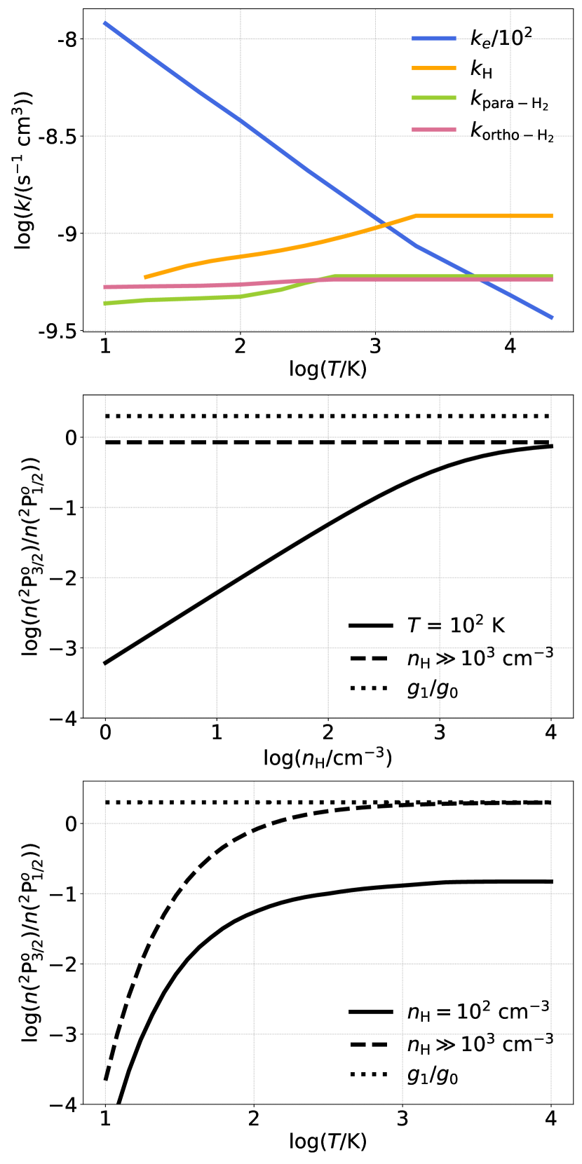
Figure 1.— Top panel - collisional rate coefficients from the LAMDA database for electrons, H, ortho- and para-H₂. Middle panel - the relative abundance of the excited C⁺ level ${}^{2}\rm{P}_{3/2}^{\rm{o}}$ as a function of density for a fixed temperature of $T=100$ K, assuming abundances of $x_{\rm{H}}=0.5$, $x_{\rm{e}}=10^{-4}$, $x_{\rm{H}_{2}}=0.25$, the ratio for a thermalized population $g_{1}/g_{0}\times e^{-T_{10}/T}$, and the high temperature limit $g_{1}/g_{0}$. Bottom panel - as for the middle panel but showing the temperature dependence for a fixed H nucleus density.

The middle panel of Figure 1 shows the density dependence of the excitation state of C⁺ for a fixed temperature of 100 K, assuming abundances of $x_{\rm{H}}=0.5$, $x_{\rm{e}}=10^{-4}$, $x_{\rm{H}_{2}}=0.25$, and an orth-to-para H₂ ratio of 3, representing typical conditions in the cold ISM. Also plotted is the asymptotic value for $n\gg 10^{3}$ cm^-3, given by the Boltzmann factor $g_{1}/g_{0}\times\exp{(-T/T_{10})}$, and the high temperature limit $g_{1}/g_{0}$, where $g_{1}$ and $g_{0}$ are the statistical weights for the upper and lower excitation states, respectively, and $T_{10}$ is the temperature corresponding the the transition energy. The density dependence of the excitation state begins flattening at $n\sim 10^{3}$ cm^-3, corresponding to the critical density of the transition. The bottom panel of Figure 1 shows the temperature dependence of the excitation state of C⁺ for the same chemical abundances, for a density of $n=10^{2}$ cm^-3 and $n\gg 10^{3}$ cm^-3, as well as the high temperature limit. The temperature dependence is weak when $T\gtrsim 100$ K, corresponding to the temperature of the transition at 91.21 K.

4. Overview of Simulation Results

4.1. Metallicity Dependence

Figure 2 shows the metallicity dependence of the time averaged H₂ column, $[\rm{CII}]$ intensity $W_{\rm{[CII]}}$, the conversion factor $X_{\rm{[CII]}}$ (see Equation 2), and the fraction of $n>10\;\rm{cm}^{-3}$ carbon mass in the form of C⁺, denoted as $f_{\rm{C}^{+}}$. Also presented are calculations of $X_{\rm{[CII]}}$ from Madden et al. (2020) and Ebagezio et al. (2022). The almost linear rise of $W_{\rm{[CII]}}$ can be understood by the fact that the emission is approximately optically thin, and that C⁺ mass scales approximately linearly with metallicity. As is described in further detail in Section 4.3, [CII] emission in our calculations originates mostly from dense ($n>10~{}\rm{cm}^{-3}$) gas. As a larger fraction of the dense carbon is in the form of C and CO due to an increase in dust shielding, the fraction of dense C⁺ is expected to decrease, but as can be seen in Figure 2, this effect is almost negligible. $N_{\rm{H}_{2}}$ increases with metallicity due the combined effect of increased dust shielding and H₂ formation on dust grains. Averaged over time, this effect turns out to be close to linear. Given these effects, the [CII]-to-H₂ conversion factor is almost constant with metallicity, with its slight increase attributed to the decrease in $f_{\rm{C}^{+}}$. It is well fitted by the power law $X_{\rm{[CII]}}=6.31\times 10^{19}\;Z^{\prime\;0.17}\;(\rm{cm}^{-2}\;(\rm{K}\;\rm{km}\;\rm{s}^{-1})^{-1})$, which describes our results with an accuracy of $<5\%$.

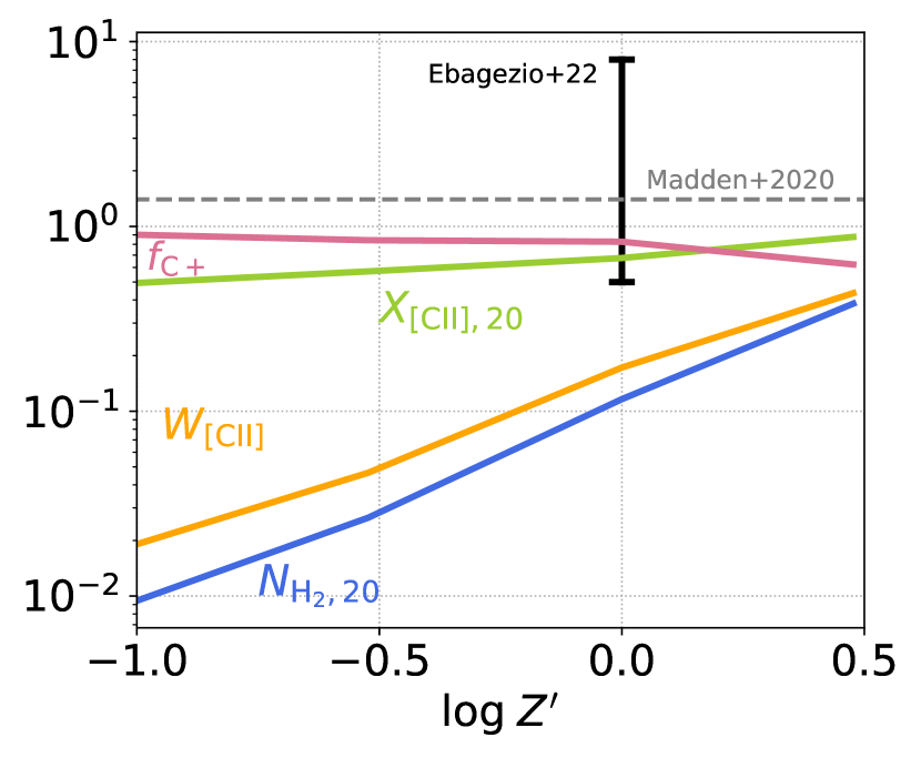
Figure 2.— Time average of $W_{\rm{[CII]}}$ (K km s^-1), $X_{\rm{[CII]},20}\equiv X_{\rm{[CII]}}/(10^{20}\;\rm{K\;km\;s}^{-1})$, $N_{\rm{H}_{2},20}\equiv N_{\rm{H}_{2}}/(10^{20}\;\rm{cm}^{-2})$, and $f_{\rm{C}^{+}}\equiv M_{\rm{C}^{+}}/{M_{\rm{C,tot}}(n>10\;\rm{cm}^{-3})}$. Also shown are the values of $X_{\rm{[CII]},20}$ from Madden et al. (2020) and Ebagezio et al. (2022). $W_{\rm{[CII]}}$ and $N_{\rm{H}_{2}}$ increase almost linearly with metallicity. The weak metallicity dependence of $X_{\rm{[CII]}}$ is explained by the slight decrease in $f_{\rm{C}^{+}}$.

4.2. Column Density and Emission Maps

Figure 3 shows a series of total gas column density maps for the $Z^{\prime}=1$ run at different times. The life cycle of the ISM is evident. At $t=340$ Myr, the ISM consists of a mostly diffuse medium, with a few small, dense clumps just above and to the right of the image center. Gas cools and accumulates as the clumps grow, until at $t=400$ Myr a dense cloud is fully formed and is visible in the center of the image. As the clouds condense and cool, stars begin to form in the densest regions. The more massive OB stars ionize their surroundings, and once they explode the energy injected into the surrounding gas causes the cloud to disperse, as is visible in the $t=430$ Myr snapshot. This cycle generally repeats and gives a qualitative understanding of the time evolution of the HSvD21 simulations.

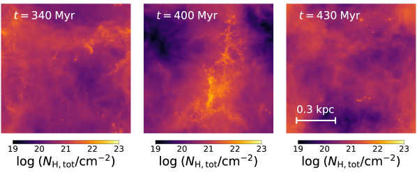
Figure 3.— Maps of total column density for the $Z^{\prime}=1$ run of the HSvD21 simulations, taken at $t=340$, 400, and 430 Myr, showing the effect of time evolution.

Figure 4 shows maps of H₂ and C⁺ column density, and $W_{\rm{[CII]}}$, for the $Z^{\prime}=1$ and 0.1 at $t=520$ and 230 Myr respectively. Both snapshots show a dense cloud, traced by large H₂ column densities. C⁺ is more extended, tracing both atomic and molecular gas, while the high column density sightlines trace the molecular gas.

The $[\rm{CII}]$ emission map is computed by Radmc-3D, as described in Section 2.2. The emission intensity qualitatively traces the column density, but with a larger dynamical range, showing that the [CII] intensity is biased towards dense gas. This is due to the high column density sightlines also containing high (volume) density gas, in which collisional excitation of the [CII] line is enhanced. Also visible is the further enhancement of intensity in quasi-spherical bright regions embedded within the dense cloud. These are regions where OB stars photoionize and heat up the gas, causing both an increase in the relative C⁺ abundance, as well as enhanced excitation of the [CII] line due to the increased temperature and electron fraction. These effects are discussed in detail in Section 4.3.

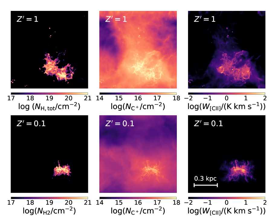
Figure 4.— H₂ and C⁺ column density maps, and [CII] emission maps for $Z^{\prime}=1$ (top row) and 0.1 (bottom row), for $t=520$ and 230 Myr, respectively. While the C⁺ distribution is extended, [CII] emission and H₂ both trace dense gas.

4.3. Chemical Properties

Since C⁺ resides in all phases of the ISM, relating [CII] emission to cold gas content and star-formation requires understanding which ISM phase dominates the [CII] emission. Panel (a) in Figure 5 shows the 2D histogram for temperature and density weighted by gas mass for the $Z^{\prime}=1$ run, using all particle data from all snapshots. A few regions of interest are clearly visible. The bright, almost horizontal strip at $\sim 10^{4}$ K extending up to $n\sim 10$ cm^-3 is the WNM, where gas temperature is almost constant across a wide range of densities due to efficient Lyman-$\alpha$ cooling. Above $n\sim 10$ cm^-3, and at lower temperatures, we can see the CNM and molecular ISM, where gas is cooled by metal fine-structure lines (mostly [CII] emission and [CI] 609 and 370 $\mu$m emission) and CO molecular line emission. The thin horizontal strip at $n\gtrsim 10$ cm^-3 is gas in HII regions, where radiation from OB stars ionizes and heats the gas to $10^{4}$ K. The gas with temperatures higher than the WNM/HII region gas is the hot ionized medium (HIM), shock heated and ionized by SNe feedback.

We define the different phases in the space of temperature and ionization fraction using the following criteria - cold gas ($T<3\times 10^{2}$ K), unstable neutral medium (UNM; $3\times 10^{2}<T<3\times 10^{3}$ K), WNM ($3\times 10^{3}<T<3\times 10^{4}$ K, $x_{e}<0.99$), HII regions ($3\times 10^{3}<T<3\times 10^{4}$ K, $x_{e}>0.99$), and HIM ($T>3\times 10^{4}$ K). We caution that we could overproduce the C⁺ abundance (and therefore [CII] emission) in both HII regions and the HIM, as carbon is expected to be (at least partially) in the form of higher ionization stages in these environments, while our chemistry treatment does not account for these. As is discussed in Section 4.3, the overproduction of [CII] in the HIM is not a concern, as the HIM is negligible compared to the other ISM phases. In HII regions, a significant fraction of the carbon is expected to be in the form of C²⁺ and C³⁺. The picture presented in Figure 5 is qualitatively similar in simulation runs with different metallicities, the main differences being a lower cold ISM temperature, and a lower transition density between WNM and CNM phases, for higher values of $Z^{\prime}$.

Panel (b) of Figure 5 shows the 2D temperature-density histogram, weighted by C⁺ mass. We see a similar pattern to that of the total gas mass histogram, the main difference being that C⁺ mass is absent in the highest density cold gas. This is due to the effect of dust- and gas self-shielding against FUV in the denser regions of gas clouds, reducing the C⁺ abundance relative to C and CO. Table 1 shows the fraction of C⁺ mass in the different ISM phases defined above. For all metallicities, most of the C⁺ mass is in the WNM, where most of the total gas mass is, and where the carbon is entirely in the form of C⁺. Another fraction of order 10% is in the cold ISM and UNM across all metallicities. A lower fraction of the mass of the order of a few % is in HII regions and the HIM. We note that our WNM mass fraction is higher than observed in studies of 21 cm self-absorption (Heiles & Troland, 2003; Stanimirović et al., 2014).

The HII region mass fraction is higher for higher metallicity. This can be understood by the fact that the mass of a classical Stromgren sphere around an ionizing source with a given ionizing photon production rate is inversely proportional to gas density. Since the cold ISM cools via line emission from different metal species, it is colder at higher metallicity. This leads to gas reaching the threshold for star formation at lower density, driving down the average density of HII regions as a result. Indeed, the average density of HII regions in our simulations is 28.97, 12.85, 10.06, and 4.61 cm^-3, for the $Z^{\prime}=$0.1, 0.3, 1, and 3 runs respectively.

Panel (c) of Figure 5 shows the density-temperature histogram weighted by [CII] emissivity. The emissivity of each particle is computed by finding the excitation state of C⁺ using the density, temperature, and chemical abundances computed in HSvD21, as well as using collisional rate coefficients from the LAMDA database, as is used by Radmc-3D. In this calculation, we assume no radiation trapping, and by using this 3D information regarding [CII] emission we are implicitly assuming that the emission is optically thin. In panel (d) of Figure 5 we show the C⁺ mass- and [CII] emissivity-weighted volume density cumulative distribution function, demonstrating the [CII] emission originates in dense ($\gtrsim 10$ cm^-3) gas, while C⁺ is distributed over a larger density range.

As we show in Section 6, [CII] is only marginally optically thick at $Z^{\prime}=3$, and optical depth effects are completely negligible at $Z^{\prime}\leq 1$, which validates our discussion of 3D emissivity data. It is clear that while C⁺ mass resides predominantly in the WNM, [CII] emission originates from cold gas and HII regions, i.e. dense gas. While the fraction of C⁺ mass in dense gas (cold ISM, UNM, and dense HII regions) is only of order 10%, the density, being larger by an order of magnitude, enhances the excitation of C⁺ by an order of magnitude (see Figure 1) and thus increases the emissivity by two orders of magnitude.

Table 2 shows the fraction of [CII] emissivity originating in the different ISM phases. It can be seen that while most of the C⁺ mass is the WNM, its contribution to [CII] emission is of order 1%. Cold gas, on the other hand, contributes over half of the emissivity at $Z^{\prime}=0.1$, decreasing with metallicity down to 19% at $Z^{\prime}=3$. This is due to photoionization feedback from star formation being more efficient at ionizing large gas masses, owing to the lower density of HII regions at high metallicity. This leads to the growth of the HII region mass fraction at the expense of CNM and molecular ISM mass. HII regions, while contributing only $\sim$1% of the C⁺ mass, contribute over 30% of the emission at $Z^{\prime}=0.1$ and increase with metallicity up to 79% at $Z^{\prime}=3$. This is due to a combination of photoionization heating increasing gas temperature, as well as an increased electron abundance compared to the WNM/CNM. As the rate coefficient with electrons at this temperature is larger than for collisions with H₂, this causes an increase in [CII] emissivity by two orders of magnitude relative to cold ISM conditions. Ebagezio et al. (2022) use tabulated CLOUDY models to test the effect of stellar photoionization feedback on the [CII] luminosity in HII regions and find that the [CII] luminosity is reduced by up to 60% due to ionization of C⁺ to higher ions. Applying this result to our time-averaged results for [CII] intensity, this would lead to a reduction of between 13 and 31.5%, depending on metallicity. HIM contribution is to [CII] is negligible, as expected since HIM is both low mass and diffuse.

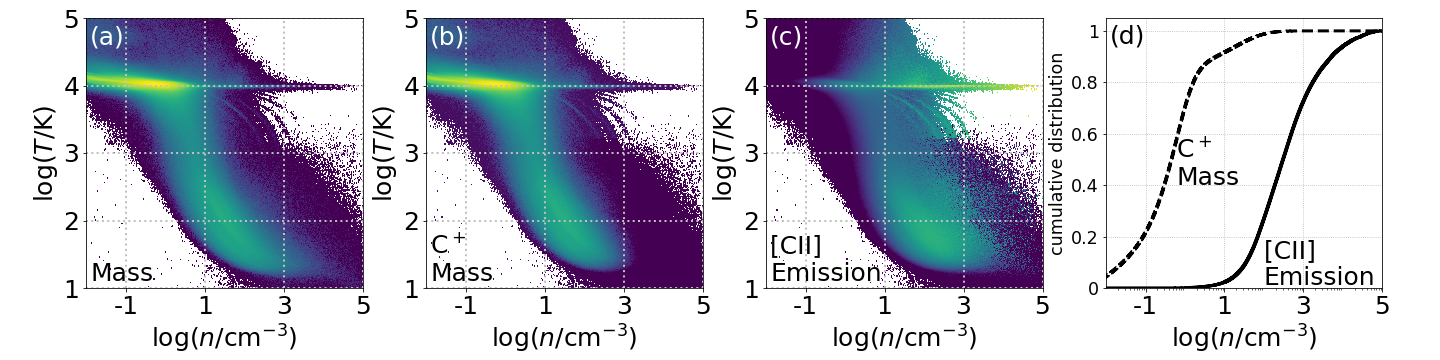
Figure 5.— 2D histograms in density and temperature for gas mass (panel (a)), C⁺ mass (panel (b)), and [CII] emissivity (panel (c)). Panel (d) shows the C⁺ mass- and [CII] emissivity-weighted cumulative density distribution.

Table 1Fractions of C⁺ mass in different ISM phases

Phase	$Z^{\prime}=0.1$	0.3	1	3
Cold Gas	0.038	0.055	0.112	0.142
UNM	0.088	0.057	0.033	0.063
WNM	0.844	0.850	0.855	0.746
HII regions	0.004	0.005	0.009	0.016
HIM	0.026	0.032	0.023	0.034

Table 2Fractions of [CII] from different ISM phases

Phase	$Z^{\prime}=0.1$	0.3	1	3
Cold gas	0.58	0.46	0.29	0.18
UNM	0.06	0.03	0.03	$<$0.02
WNM	0.03	0.02	0.02	$<$0.01
HII regions	0.33	0.46	0.66	0.79
HIM	$<$0.01	0.03	$<$0.01	$<$0.01

5. Time Variation

In this section we examine the time variation of molecular gas content, star formation rate (SFR), and [CII] emission. The top panel of Figure 6 shows the time dependence of SFR, H₂ column density, and [CII] emission, averaged over the entire box at each time step. All three quantities peak at similar times, with SFR falling more dramatically. This is qualitatively understood by a cycle of cloud gravitational collapse followed by stellar feedback, as is demonstrated in Figure 3. The gravitational collapse leads to an enhancement of both density and effective shielding column of the gas. This in turn increases the H₂ formation rate and lowers the FUV intensity, leading to high H₂ column densities. The density enhancement also increases the [CII] intensity, due to an increased excitation of the upper energy level. The SFR rises as more gas cools and compresses to pass our SF threshold. The rise in SFR triggers photoionization feedback which affects nearby gas. This causes an increase in gas temperature, photodissociation of H₂ and CO, and photoionization of C. This leads to a drop in H₂ abundance, as well as a short-lived increase in [CII] intensity due to the increased temperature and electron fraction in the HII region, followed by dispersal of the dense gas by SN feedback, which lowers the [CII] intensity.

This cycle is further demonstrated in the top panel of Figure 7, where we present the fraction of [CII] emission coming from the different gas phases. The peaks in SFR correspond to peaks in HII region relative emission, while the drops correspond to cold gas dominated emission. HIM and WNM never contribute significantly to [CII] emission. In comparison, the $Z^{\prime}=0.1$ run shows different behavior. As is discussed in HSvD21, the cooling time is longer in lower metallicity gas, leading to burstier and more clustered star formation, and accordingly long periods of quiescence. This is demonstrated in the bottom panel of Figure 6, showing the steep drop (and vanishing) of SFR between star-formation episodes, while [CII] emission drops much less dramatically to a floor value. During this period of low SFR, the gas remains in predominantly WNM form, leading to reduced emission due to decreased density, but this decrease is not as dramatic as the drop in SFR. This is further demonstrated in the bottom panel of Figure 7, where cold gas dominated emission corresponds to episodes of star-formation, while WNM dominates emission intermittently between the episodes. It should be noted that while high SFR corresponds to [CII] emission from dense gas, it corresponds to emission from HII regions in the $Z^{\prime}=1$ run, while in the $Z^{\prime}=0.1$ run, it corresponds to cold gas dominated emission, as is discussed in Section 4.3.

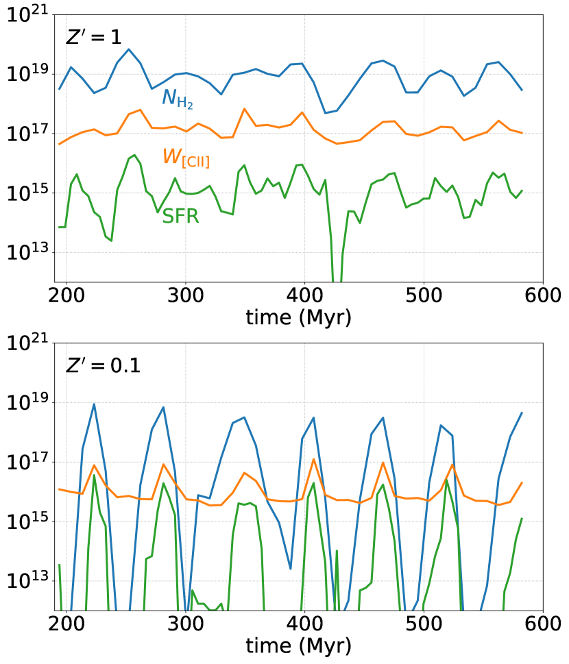
Figure 6.— Time dependence of SFR/$(10^{-18}\;M_{\odot}\;\rm{yr}^{-1})$, $N_{\rm{H}_{2}}/(\rm{cm}^{-2})$, and $(W_{\rm{[CII]}}/(10^{-18}\;\rm{K\;km\;s}^{-1}))$, for the $Z^{\prime}=1$ (top panel) and $Z^{\prime}=0.1$ (bottom panel) runs.

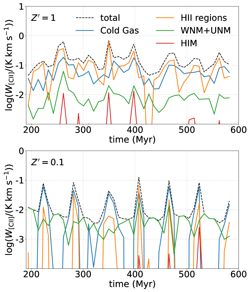
Figure 7.— Time dependence of [CII] intensity originating from different gas phases: Total intensity, Cold gas (log $T<2.5$), warm neutral medium (including the theramally unstable neutral medium; $2.5<$log$\;T<4.5$, $x_{e}<0.99$), hot ionized medium (HIM; log $T>$4.5), and HII regions ($3.5<$log $T<4.5$, $x_{e}>0.99$) for the $Z^{\prime}=1$ (top panel) and $Z^{\prime}=0.1$ (bottom panel) runs.

5.1. SFR-$W_{[CII]}$ Relation

While a qualitative picture of the relationship between SFR and [CII] emission is established in the previous section, a more quantitative approach is necessary to test theory against observations. To this end, we present in Figure 8 the [CII] luminosity, $L_{\rm{[CII]}}$ vs. star formation rate. $L_{\rm{[CII]}}$ is computed by averaging the line integrated intensity $<I_{\rm{[CII]}}>$ as computed by Radmc-3D, and then assuming that the radiation is isotropic over a sphere of radius 1 kpc, which is our box side length

$$L_{\rm{[CII]}}\equiv 4\pi(1~{}{\rm kpc})^{2}<I_{\rm{[CII]}}>.$$ (4)

Since the relationship between these quantities is usually measured on galactic scales (except for observations of nearby galaxies), we use a stack of galaxy patches, i.e. a sum of $L_{\rm{[CII]}}$ and SFR over 21 snapshots. This is done in order to allow the strong temporal variations in our box to average out as they would on the scale of a galaxy, where we do not expect the ISM across the entire galaxy to be collapsing, forming stars, and dispersing in unison. We also present the full stack of all 41 snapshots for each metallicity, represented by a star in a corresponding color. Also plotted are fits to observations of different surveys of both local (De Looze et al., 2011, 2014; Herrera-Camus et al., 2015) and high-redshift galaxies (Schaerer et al., 2020).

A positive trend in the $L_{\rm{[CII]}}$-SFR relation is visible for all metallicities, while the normalization is higher at higher metallicity. The scatter is also larger at lower metallicity, due to time variability in these runs being larger than the high metallicity runs. The slope for the $Z^{\prime}=1$ and 3 runs is close to linear. The $Z^{\prime}=0.1$ and 0.3 runs show a linear trend at high SFR, but seem to flatten at lower values. This can be explained by the longer cooling time of the low-metallicity runs, which leads to extended periods during which cold, dense gas is absent. This can be seen in the lower panel of Figure 6, where $W_{\rm{[CII]}}$ hits a floor value when the SFR vanishes. This floor value is associated with WNM emission, as can be seen in the lower panel of Figure 7. The higher normalization of the different $L_{\rm{[CII]}}$-SFR relation can be understood in two ways. First, as is described in Section 4, the total [CII] luminosity increases almost linearly with metallicity, simply due to an increase in the carbon abundance, while the median SFR is constant with metallicity (see HSvD21). Second. one can understand the increase in the normalization of the relation using an energetics argument. The CNM is heated mainly by dust photoelectric heating, whose abundance scales linearly with metallicity in our simulations, while cooling is dominated by [CII] emission. Heating also scales with FUV intensity, which scales with SFR, so for a constant SFR across all metallicities, we expect [CII] emission to increase linearly to compensate for the increase in photoelectric heating.

In the right panel of Figure 8 we show that the stack of all 41 snapshots compared to fits to observational surveys. All but the $Z^{\prime}=0.1$ data points are within the scatter of the observational data. We mention that our SFR values fall on the low end of the local surveys of De Looze et al. (2011), De Looze et al. (2014), and Herrera-Camus et al. (2015), while the comparison with data from the high-redshift survey of Schaerer et al. (2020) requires an extrapolation of their results, as they do not observe [CII] emission in galaxies with SFR $\lesssim 1\;M_{\odot}\;\rm{yr}^{-1}$. Importantly, our simulation has a fixed setup and initial conditions, while the metallicity is systematically varied. While this is insightful, it does not take into account observed and theoretically predicted correlations between gas metallicity and other galaxy properties, namely stellar mass, which is in turn related to the gas surface density and specific SFR.

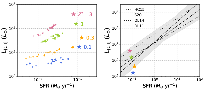
Figure 8.— Left panel: $L_{\rm{[CII]}}$ vs. SFR, for stacks of 21 snapshots. Stars show stacking of all 41 snapshots for metallicity of the respective color. Right panel: same stars as for left panel, and fits to observations of De Looze et al. (2011) sample of $z=0$ galaxies, De Looze et al. (2014) $z=0$ dwarf galaxy survey, Herrera-Camus et al. (2015) KINGFISH survey, and Schaerer et al. (2020) ALMA-ALPINE survey of $z\sim 4-8$ galaxies. The shaded area represents the union of 1 $\sigma$ scatter across all surveys.

We stress that while stacking our snapshots allows for the averaging out of the temporal scatter in this relation, a more elaborate setup is required in order to fully investigate this relationship on a galactic scale. This is because our box has an average gas surface density corresponding to the solar neighbourhood and a fixed metallicity, while a full galaxy is expected to have a radial variation in both gas surface density and gas metallicity, requiring a stack of many boxes with different gas properties in order to get a picture of the $L_{\rm{[CII]}}$-SFR on galactic scales.

6. Optical Depth

6.1. Optically Thin Calculation

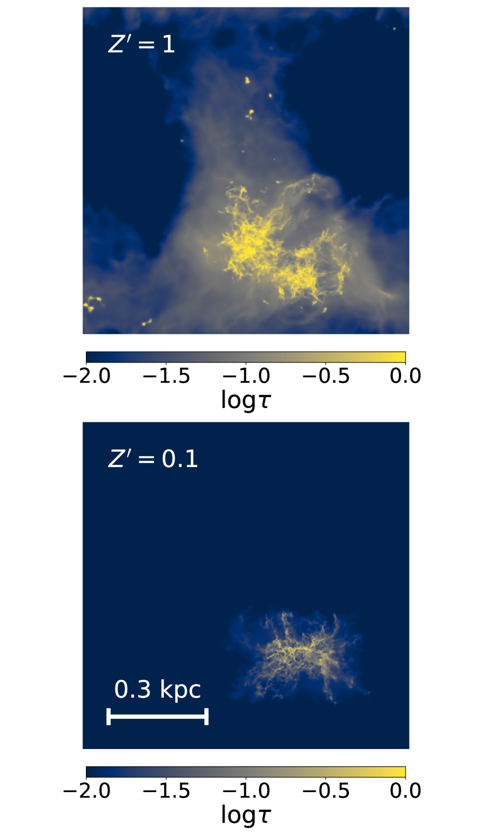
Figure 9.— Maps of projected [CII] optical depth for the $Z^{\prime}=1$ (top panel) and 0.1 (bottom panel), for $t=520$ and 230 Myr respectively.

To investigate the effects of optical depth on our results, and validate our numerical computations, we compare the results computed using Radmc-3D with an independent optically thin calculation. We compute the [CII] emissivity for each cell in the AMR grid, by neglecting absorption and stimulated emission, and using the temperature, density, and chemical abundances calculated in the simulation, as well as the rate coefficients from the LAMDA database. The emissivity is given by

$$j_{10}=n_{1}A_{10}E_{10},$$ (5)

where $n_{1}$ is the density of excited C⁺, $A_{10}$ is the Einstein coefficient for spontaneous emission, and $E_{10}$ is the transition energy. For a two-level system such as C⁺, $n_{1}$ can be calculated simply using

$$\frac{n_{1}}{n_{0}}=\frac{R_{01}}{R_{10}}=\frac{\sum_{i}k_{01,i}n_{i}}{\sum_{i}k_{10,i}n_{i}+A_{10}},$$ (6)

where $n_{0}$ is the density of the lower excitation state of C⁺, $n_{i}$ is the density of collision partner $i$, and $k_{01,i}$ ($k_{10,i}$) is the upwards (downwards) collisional rate coefficient with collision partner $i$. $R_{ij}$ is the rate of transitions from level $i$ to level $j$.

We then project the emissivities onto a 512x512 grid, effectively creating an optically thin image of the line integrated intensity.

In addition, we compute the optical depth for each cell given by

$$\frac{d\tau_{10}}{dz}=\frac{\lambda_{10}^{3}A_{10}g_{1}}{8\pi^{3/2}g_{0}}\Big{(}\frac{n_{0}}{b}(1-\frac{n_{1}g_{0}}{n_{0}g_{1}})\Big{)},$$ (7)

where $\lambda_{10}$ is the wavelength of the [CII] line, $g_{1}$ ($g_{0}$) is the statistical weight of the upper (lower) excitation stat of C⁺, and $b$ is the Doppler broadening parameter. $b$ is calculated using

$$b^{2}=b_{\rm{turb}}^{2}+b_{\rm{therm}}^{2}=b_{\rm{turb}}^{2}+\frac{k_{B}T}{\mu m_{p}},$$ (8)

where $b_{\rm{turb}}$ and $b_{\rm{therm}}$ are the turbulent and thermal broadening parameters, respectively, $k_{B}$ is the Boltzmann constant, $\mu$ is the mean molecular weight, and $m_{p}$ is the proton mass. We then project $d\tau_{10}/{dz}$ onto the same grid and create a map of the optical depth $\tau_{10}$. In Figure 9 we show sample optical depth maps for the snapshots presented and discussed in Section 4.2. In the $Z^{\prime}=1$ case, $\tau_{10}\ll 1$ for sightlines outside of the dense cloud. In the densest regions, however, $\tau_{10}$ reaches unity. In the $Z^{\prime}=0.1$ case, $\tau_{10}$ is small everywhere. Our computation of the optical depth is an upper limit, and in fact, is an overestimation in the high $W_{\rm{[CII]}}$ sightlines by $\sim$0.5 dex. The origin of this overestimation is due to Radmc-3D taking into account the bulk velocity of the gas particles, which can allow radiation to escape freely through a high column density sightline. Discussion of this effect, as well as a more detailed comparison between our optically thin calculation and Radmc-3D, can be found in Appendix A. The comparison shows a good agreement between Radmc-3D and our optically thin calculation in the optically thin sightlines, and the difference between the two in the optically thick regime can be explained by the optical depth calculation.

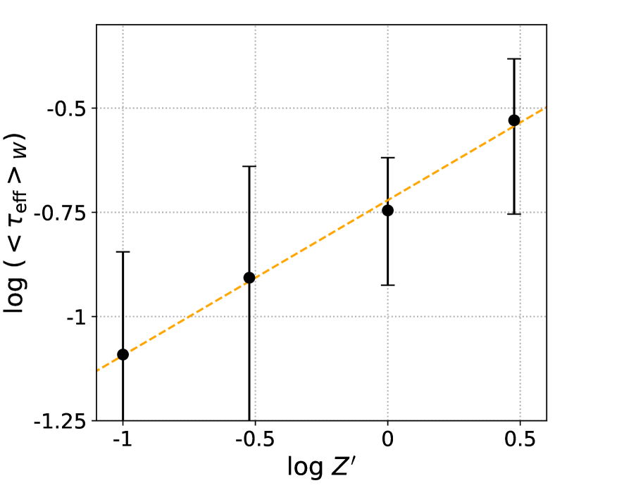
Figure 10.— Effective intensity-weighted [CII] optical depth averaged over the entire simulation run. as a function of gas metallicity. Error bars represent the standard deviation of the 41 snapshots averaged for each simulation run.

Given the agreement between our optically thin calculation and the full radiative transfer, we can justify our calculations in Section 4.3 based on the computed 3D emissivity. In addition, we can now investigate the optical depth of [CII] emission in our simulation.

6.2. Optical Depth Effect

Given that we overestimate optical depth at the high end by approximately 0.5 dex, we opt for a more accurate estimation of optical depth. We define the effective optical depth by the equation

$$\frac{1-e^{-\tau_{\rm{eff}}}}{\tau_{\rm{{eff}}}}=\frac{W_{\rm{[CII],RADMC-3D}}}{W_{\rm{[CII],thin}}},$$ (9)

where $W_{\rm{[CII],RADMC-3D}}$ and $W_{\rm{[CII],thin}}$ are the values for $W_{\rm{[CII]}}$ in our full radiative transfer and optically thin calculation, respectively. This definition is motivated by the solution of the radiative transfer equation for a static, uniform medium with source function $S$, no background radiation, and optical depth $\tau$. The full solution results in an intensity

$$I=S(1-e^{-\tau}),$$ (10)

while the solution for the optically thin limit gives

$$I_{\rm{thin}}=S\tau,$$ (11)

and the ratio between the two solutions is given by the expression in Equation 9, replacing $\tau_{\rm{eff}}$ with $\tau$.

For each simulation snapshot, we then compute the intensity weighted average over all pixels in the snapshot

$$<\tau_{\rm{eff}}>_{W}\equiv\frac{\sum W_{i}\tau_{\rm{eff},i}}{\sum W_{i}}.$$ (12)

Figure 10 shows the time average of $<\tau_{\rm{eff}}>_{W}$ as a function of metallicity. Importantly, we find that for the gas surface density in our simulations, the gas only just approaches the regime where optical depth effects are important at $Z^{\prime}=3$, where the time-averaged effective optical depth gives an optically thin intensity stronger by only  15%. We present a power law fit to our data of the form

$$\mathrm{log}(<\tau_{\mathrm{eff}}>)=0.37\times\mathrm{log}Z^{\prime}-0.72.$$ (13)

This gives the result that [CII] emission can be assumed to be (approximately) optically thin up to solar metallicity (at all metallicities), given a gas surface density of 10 $M_{\odot}$ pc^-2. It is highly probable that this result will not hold in environments where gas surface densities are higher by an order of magnitude or more, which should scale the optical depth by the same factor.

7. Summary

We have presented radiative transfer calculations of [CII] intensity using Radmc-3D and applying it to a set of sub-pc resolution hydrodynamical simulations of a self-regulated, SN driven ISM. We investigate the systematic effects of metallicity on line intensity over a large range $0.1\leq Z^{\prime}\leq 3$, and the intensity contribution of different ISM phases. Our simulation time (500 Myr) and volume ($1\times 1\times 10$ kpc³) are large enough to allow us to understand the spatial and temporal variations in [CII] intensity and its correlation with SFR and molecular gas content. We summarize our main results below:

1. The time-averaged [CII] line luminosity on kpc scales grows approximately linearly with metallicity at all but super-solar metallicities (see Figure 2). This effect is simply a column density effect, as most of the carbon mass is in the form of C⁺, and the emission is approximately optically thin, especially in the sub-solar metallicity cases.

2. The spatially averaged [CII] luminosity correlates with SFR, as long as it is dominated by cold gas, with a potential contribution from HII regions. We find a linear $L_{\rm{[CII]}}$-SFR relation, with a normalization proportional to metallicity (see left panel of Figure 8). This is due to both dust photoelectric heating and C⁺ emissivity scaling linearly with metallicity. This is also explained by SFR correlating with the gravitational collapse and clumping of gas, which in turn enhances collisional excitation and, in turn, emissivity. While we only simulate a small region relative to galactic scales, summing our [CII] luminosities and SFR values results in an agreement with the observed relation (within their scatter) in all but the lowest metallicity (see right panel of Figure 8).

3. The majority of [CII] emission originates from high-density gas ($n>10^{2}~{}{\rm cm^{-3}}$), highlighting the need to resolve the small-scale clumpy structure of the ISM to realistically capture the [CII] line.

4. We find that different phases of the ISM dominate emission at different times (see Figure 7, Table 2). Over the entire simulation run, it is the cold gas and HII regions that dominate emission, as their higher density enhances the excitation of the [CII] line. Lower luminosities associated with the lowest SFRs ($\lesssim 10^{-2}\;M_{\odot}$ yr^-1) represent a floor value that is dominated by WNM emission, and no longer correlates with SFR. This regime is only explored in the sub-solar metallicity runs, as longer cooling times lead to extended periods in which dense gas is absent. We caution that our treatment of emission from HII regions does not include higher ionization stages of carbon and emission from HII regions is overproduced by up to a factor of $\sim$2.

5. [CII] emission traces H₂ (see Figure 2), for the same reasons that it traces SFR. The metallicity dependence of the conversion factor $X_{[\rm{CII]}}$ is weak, ranging from 5 to 9$\times 10^{19}$ cm^-2/(K km s^-1). This is due to [CII] luminosity and H₂ column density having a similar scaling with metallicity. In conjunction with our findings that [CII] emission is dominated by dense gas, this is evidence in support of using [CII] as a tracer for molecular gas content. Our results are fit well by the power law $X_{\rm{[CII]}}=6.31\times 10^{19}\;Z^{\prime\;0.17}\;(\rm{cm}^{-2}\;(\rm{K}\;\rm{km}\;\rm{s}^{-1})^{-1})$. For solar metallicity, we find agreement between our results and Ebagezio et al. (2022). The result of Madden et al. (2020) is based on observations over a large range of metallicities, from $Z^{\prime}=0.02$ up to $\sim 1$, and is in agreement with result to within a factor of $\sim 2$.

6. Our simulations are all run with identical gas surface density in order to allow for a systematic investigation of the effects of metallicity. We find different $L_{\rm{[CII]}}$-SFR relations for different metallicities, while observations seemingly find a single relation independent of metallicity. This could be due to the fact that as galaxies evolve, both its metallicity and gas surface density are expected to change, while we did not study the effect of varying gas surface density.

7. By carefully comparing a full radiative transfer treatment with our own optically thin calculation, we are able to quantify the effective optical depth, accounting for absorption, relative bulk motion, and line-broadening (see Figure 10). We find that for average gas surface density of $\Sigma=10\;M_{\odot}$ pc^-2, [CII] emission can be treated as optically thin except for the most extreme cases in our $Z^{\prime}=3$ run, where $\tau\sim 0.3$.

We thank Chris McKee and Reinhard Genzel for fruitful discussions. This work was supported by the German Science Foundation via DFG/DIP grant STE/1869-2 GE 625/17-1, by the Center for Computational Astrophysics (CCA) of the Flatiron Institute, and the Mathematics and Physical Sciences (MPS) division of the Simons Foundation, USA.

Appendix A - Comparison Between Radmc-3D and The Optically Thin Calculation

In this appendix, we describe in detail our comparison between the optically thin calculation and Radmc-3D. Figure 11 shows the ratio between the Radmc-3D calculation and the optically thin calculation as a function of optical depth, for the $Z^{\prime}=1$ and 0.1 at $t=520$ and 230 Myr respectively, using three different methods. The left column shows the result using our default settings on Radmc-3D, as described in Section 2.2. The middle column shows the same calculation as (a) but with the bulk velocity of all particles set to 0, and Radmc-3D line transfer mode set to ”optically thin”. We stress that this line transfer mode does not ignore absorption, but the ”optically thin” term here refers to the calculation of the local level populations assuming no line trapping, as opposed to our default settings where line trapping is taken into account using the LVG approximation. The right column shows the same calculation, but this time the wavelength range covered by Radmc-3D when integrating over the [CII] line was set to 300 instead of 20 km s^-1, and again using ”optically thin” line transfer mode in Radmc-3D. All panels show the curve

$$\frac{I_{\rm{thin}}}{I_{\rm{fullRT}}}=\frac{\tau}{1-e^{-\tau}},$$ (14)

as is the case for a uniform slab. The default settings show good agreement at intermediate optical depth, but an overestimation of optically thin emission at both low and high optical depth. The middle column shows that when the bulk velocity of the gas is set to 0, the overestimation of optical depth in the optically thin calculation is mitigated. This shows that the default comparison suffers from an overestimation of optical depth, due to neglecting the relative bulk motion of the gas in the optically thin calculation. The turning off of LVG mode here was in order to avoid numerical problems that arise from computing the velocity gradient when the velocities are set to 0 everywhere. The right column shows that the disagreement at low optical depth is a result of the low optical depth sightlines containing gas with a large linewidth, as well as possibly large bulk motions. This causes a significant fraction of the emission to be missed by Radmc-3D during integration, as line emission is either broadened or shifted out of the integration window, and to an underestimation of emission. Since these low optical depth sightlines are made up of very low density and low column density gas, their intensity is low and this difference does not affect our results in a significant way when averaged over an entire snapshot. Overall, our optically thin calculation reproduces the Radmc-3D calculation well, and overproduces emission to the expected extent.

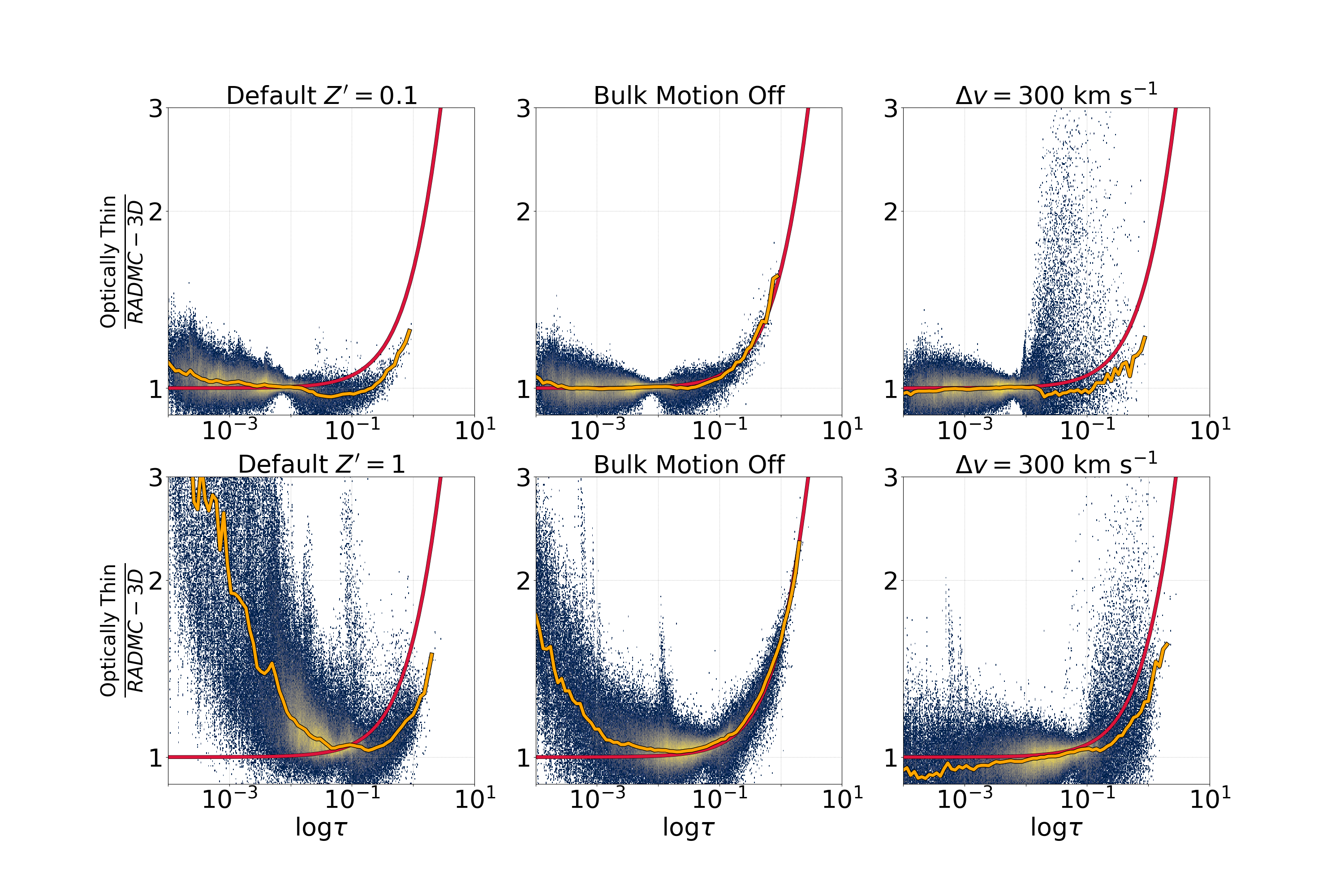
Figure 11.— Pixel-by-pixel ratio between our optically thin calculation and the full Radmc-3D calculation as a function of projected optical depth for our default settings (left panel), the linewidth set to 200 km s^-1 (middle panel), and with gas velocity set to 0 (right panel). The green curve shows the value theoretical value computed for a uniform gas mix.

References

- Barinovs et al. (2005) Barinovs, G., van Hemert, M. C., Krems, R., & Dalgarno, A. 2005, ApJ, 620, 537
- Bialy & Sternberg (2019) Bialy, S. & Sternberg, A. 2019, ApJ, 881, 160
- Bisbas et al. (2022) Bisbas, T. G., Walch, S., Naab, T., Lahén, N., Herrera-Camus, R., Steinwandel, U. P., Fotopoulou, C. M., Hu, C.-Y., & Johansson, P. H. 2022, ApJ, 934, 115
- Bolatto et al. (2013) Bolatto, A. D., Wolfire, M., & Leroy, A. K. 2013, ARA&A, 51, 207
- Bouwens et al. (2022) Bouwens, R. J., Smit, R., Schouws, S., Stefanon, M., Bowler, R., Endsley, R., Gonzalez, V., Inami, H., Stark, D., Oesch, P., Hodge, J., Aravena, M., da Cunha, E., Dayal, P., de Looze, I., Ferrara, A., Fudamoto, Y., Graziani, L., Li, C., Nanayakkara, T., Pallottini, A., Schneider, R., Sommovigo, L., Topping, M., van der Werf, P., Algera, H., Barrufet, L., Hygate, A., Labbé, I., Riechers, D., & Witstok, J. 2022, ApJ, 931, 160
- Crawford et al. (1985) Crawford, M. K., Genzel, R., Townes, C. H., & Watson, D. M. 1985, ApJ, 291, 755
- Dalgarno & McCray (1972) Dalgarno, A. & McCray, R. A. 1972, ARA&A, 10, 375
- De Looze et al. (2011) De Looze, I., Baes, M., Bendo, G. J., Cortese, L., & Fritz, J. 2011, MNRAS, 416, 2712
- De Looze et al. (2014) De Looze, I., Cormier, D., Lebouteiller, V., Madden, S., Baes, M., Bendo, G. J., Boquien, M., Boselli, A., Clements, D. L., Cortese, L., Cooray, A., Galametz, M., Galliano, F., Graciá-Carpio, J., Isaak, K., Karczewski, O. Ł., Parkin, T. J., Pellegrini, E. W., Rémy-Ruyer, A., Spinoglio, L., Smith, M. W. L., & Sturm, E. 2014, A&A, 568, A62
- Draine (1978) Draine, B. T. 1978, ApJS, 36, 595
- Dullemond et al. (2012) Dullemond, C. P., Juhasz, A., Pohl, A., Sereshti, F., Shetty, R., Peters, T., Commercon, B., & Flock, M. 2012, RADMC-3D: A multi-purpose radiative transfer tool
- Ebagezio et al. (2022) Ebagezio, S., Seifried, D., Walch, S., Nürnberger, P. C., Rathjen, T. E., & Naab, T. 2022, arXiv e-prints, arXiv:2206.06393
- Ferland et al. (2017) Ferland, G. J., Chatzikos, M., Guzmán, F., Lykins, M. L., van Hoof, P. A. M., Williams, R. J. R., Abel, N. P., Badnell, N. R., Keenan, F. P., Porter, R. L., & Stancil, P. C. 2017, RMxAA, 53, 385
- Field et al. (1969) Field, G. B., Goldsmith, D. W., & Habing, H. J. 1969, ApJ, 155, L149
- Franeck et al. (2018) Franeck, A., Walch, S., Seifried, D., Clarke, S. D., Ossenkopf-Okada, V., Glover, S. C. O., Klessen, R. S., Girichidis, P., Naab, T., Wünsch, R., Clark, P. C., Pellegrini, E., & Peters, T. 2018, MNRAS, 481, 4277
- Gaburov & Nitadori (2011) Gaburov, E. & Nitadori, K. 2011, MNRAS, 414, 129
- Galli & Palla (2013) Galli, D. & Palla, F. 2013, ARA&A, 51, 163
- Glover & Clark (2012) Glover, S. C. O. & Clark, P. C. 2012, MNRAS, 421, 116
- Glover & Mac Low (2007) Glover, S. C. O. & Mac Low, M. 2007, ApJS, 169, 239
- Górski & Hivon (2011) Górski, K. M. & Hivon, E. 2011, HEALPix: Hierarchical Equal Area isoLatitude Pixelization of a sphere, Astrophysics Source Code Library
- Harikane et al. (2020) Harikane, Y., Ouchi, M., Inoue, A. K., Matsuoka, Y., Tamura, Y., Bakx, T., Fujimoto, S., Moriwaki, K., Ono, Y., Nagao, T., Tadaki, K.-i., Kojima, T., Shibuya, T., Egami, E., Ferrara, A., Gallerani, S., Hashimoto, T., Kohno, K., Matsuda, Y., Matsuo, H., Pallottini, A., Sugahara, Y., & Vallini, L. 2020, ApJ, 896, 93
- Heiles & Troland (2003) Heiles, C. & Troland, T. H. 2003, ApJ, 586, 1067
- Herrera-Camus et al. (2015) Herrera-Camus, R., Bolatto, A. D., Wolfire, M. G., Smith, J. D., Croxall, K. V., Kennicutt, R. C., Calzetti, D., Helou, G., Walter, F., Leroy, A. K., Draine, B., Brandl, B. R., Armus, L., Sandstrom, K. M., Dale, D. A., Aniano, G., Meidt, S. E., Boquien, M., Hunt, L. K., Galametz, M., Tabatabaei, F. S., Murphy, E. J., Appleton, P., Roussel, H., Engelbracht, C., & Beirao, P. 2015, ApJ, 800, 1
- Hollenbach & Tielens (1999) Hollenbach, D. J. & Tielens, A. G. G. M. 1999, Rev. Mod. Phys., 71, 173
- Hopkins (2015) Hopkins, P. F. 2015, MNRAS, 450, 53
- Hu et al. (2017) Hu, C.-Y., Naab, T., Glover, S. C. O., Walch, S., & Clark, P. C. 2017, MNRAS, 471, 2151
- Hu et al. (2022) Hu, C.-Y., Schruba, A., Sternberg, A., & van Dishoeck, E. F. 2022, ApJ, 931, 28
- Hu et al. (2021) Hu, C.-Y., Sternberg, A., & van Dishoeck, E. F. 2021, ApJ, 920, 44
- Hu et al. (2019) Hu, C.-Y., Zhukovska, S., Somerville, R. S., & Naab, T. 2019, MNRAS, 487, 3252
- Katz et al. (2022) Katz, H., Rosdahl, J., Kimm, T., Garel, T., Blaizot, J., Haehnelt, M. G., Michel-Dansac, L., Martin-Alvarez, S., Devriendt, J., Slyz, A., Teyssier, R., Ocvirk, P., Laporte, N., & Ellis, R. 2022, MNRAS, 510, 5603
- Kroupa (2002) Kroupa, P. 2002, Sci. (New York, N.Y.), 295, 82
- Lagache et al. (2018) Lagache, G., Cousin, M., & Chatzikos, M. 2018, A&A, 609, A130
- Langer et al. (2010) Langer, W. D., Velusamy, T., Pineda, J. L., Goldsmith, P. F., Li, D., & Yorke, H. W. 2010, A&A, 521, L17
- Langer et al. (2014) Langer, W. D., Velusamy, T., Pineda, J. L., Willacy, K., & Goldsmith, P. F. 2014, A&A, 561, A122
- Le Fèvre et al. (2020) Le Fèvre, O., Béthermin, M., Faisst, A., Jones, G. C., Capak, P., Cassata, P., Silverman, J. D., Schaerer, D., Yan, L., Amorin, R., Bardelli, S., Boquien, M., Cimatti, A., Dessauges-Zavadsky, M., Giavalisco, M., Hathi, N. P., Fudamoto, Y., Fujimoto, S., Ginolfi, M., Gruppioni, C., Hemmati, S., Ibar, E., Koekemoer, A., Khusanova, Y., Lagache, G., Lemaux, B. C., Loiacono, F., Maiolino, R., Mancini, C., Narayanan, D., Morselli, L., Méndez-Hernàndez, H., Oesch, P. A., Pozzi, F., Romano, M., Riechers, D., Scoville, N., Talia, M., Tasca, L. A. M., Thomas, R., Toft, S., Vallini, L., Vergani, D., Walter, F., Zamorani, G., & Zucca, E. 2020, A&A, 643, A1
- Liang et al. (2023) Liang, L., Feldmann, R., Murray, N., Narayanan, D., Hayward, C. C., Anglés-Alcázar, D., Bassini, L., Richings, A. J., Faucher-Giguère, C.-A., Chung, D. T., Chan, J. Y. H., Çatmabacak, O., Kereš, D., & Hopkins, P. F. 2023, arXiv e-prints, arXiv:2301.04149
- Lique (2015) Lique, F. 2015, MNRAS, 453, 810
- Lupi & Bovino (2020) Lupi, A. & Bovino, S. 2020, MNRAS, 492, 2818
- Madden et al. (2020) Madden, S. C., Cormier, D., Hony, S., Lebouteiller, V., Abel, N., Galametz, M., De Looze, I., Chevance, M., Polles, F. L., Lee, M. Y., Galliano, F., Lambert-Huyghe, A., Hu, D., & Ramambason, L. 2020, A&A, 643, A141
- Madden et al. (2013) Madden, S. C., Rémy-Ruyer, A., Galametz, M., Cormier, D., Lebouteiller, V., Galliano, F., Hony, S., Bendo, G. J., Smith, M. W. L., Pohlen, M., Roussel, H., Sauvage, M., Wu, R., Sturm, E., Poglitsch, A., Contursi, A., Doublier, V., Baes, M., Barlow, M. J., Boselli, A., Boquien, M., Carlson, L. R., Ciesla, L., Cooray, A., Cortese, L., de Looze, I., Irwin, J. A., Isaak, K., Kamenetzky, J., Karczewski, O. Ł., Lu, N., MacHattie, J. A., O’Halloran, B., Parkin, T. J., Rangwala, N., Schirm, M. R. P., Schulz, B., Spinoglio, L., Vaccari, M., Wilson, C. D., & Wozniak, H. 2013, PASP, 125, 600
- McElroy et al. (2013) McElroy, D., Walsh, C., Markwick, A. J., Cordiner, M. A., Smith, K., & Millar, T. J. 2013, A&A, 550, A36
- Olsen et al. (2017) Olsen, K., Greve, T. R., Narayanan, D., Thompson, R., Davé, R., Niebla Rios, L., & Stawinski, S. 2017, ApJ, 846, 105
- Olsen et al. (2015) Olsen, K. P., Greve, T. R., Narayanan, D., Thompson, R., Toft, S., & Brinch, C. 2015, ApJ, 814, 76
- Pak et al. (1998) Pak, S., Jaffe, D. T., van Dishoeck, E. F., Johansson, L. E. B., & Booth, R. S. 1998, ApJ, 498, 735
- Parmar et al. (1991) Parmar, P. S., Lacy, J. H., & Achtermann, J. M. 1991, ApJ, 372, L25
- Pineda et al. (2013) Pineda, J. L., Langer, W. D., Velusamy, T., & Goldsmith, P. F. 2013, A&A, 554, A103
- Richter et al. (1995) Richter, M. J., Graham, J. R., Wright, G. S., Kelly, D. M., & Lacy, J. H. 1995, ApJ, 449, L83
- Schaerer et al. (2020) Schaerer, D., Ginolfi, M., Béthermin, M., Fudamoto, Y., Oesch, P. A., Le Fèvre, O., Faisst, A., Capak, P., Cassata, P., Silverman, J. D., Yan, L., Jones, G. C., Amorin, R., Bardelli, S., Boquien, M., Cimatti, A., Dessauges-Zavadsky, M., Giavalisco, M., Hathi, N. P., Fujimoto, S., Ibar, E., Koekemoer, A., Lagache, G., Lemaux, B. C., Loiacono, F., Maiolino, R., Narayanan, D., Morselli, L., Méndez-Hernàndez, H., Pozzi, F., Riechers, D., Talia, M., Toft, S., Vallini, L., Vergani, D., Zamorani, G., & Zucca, E. 2020, A&A, 643, A3
- Schöier et al. (2005) Schöier, F. L., van der Tak, F. F. S., van Dishoeck, E. F., & Black, J. H. 2005, A&A, 432, 369
- Shetty et al. (2011) Shetty, R., Glover, S. C., Dullemond, C. P., Ostriker, E. C., Harris, A. I., & Klessen, R. S. 2011, MNRAS, 415, 3253
- Springel (2005) Springel, V. 2005, MNRAS, 364, 1105
- Stanimirović et al. (2014) Stanimirović, S., Murray, C. E., Lee, M.-Y., Heiles, C., & Miller, J. 2014, ApJ, 793, 132
- Sternberg & Dalgarno (1995) Sternberg, A. & Dalgarno, A. 1995, ApJS, 99, 565
- Tielens & Hollenbach (1985) Tielens, A. G. G. M. & Hollenbach, D. 1985, ApJ, 291, 722
- Vallini et al. (2015) Vallini, L., Gallerani, S., Ferrara, A., Pallottini, A., & Yue, B. 2015, ApJ, 813, 36
- Wilson & Bell (2002) Wilson, N. J. & Bell, K. L. 2002, MNRAS, 337, 1027
- Wolfire et al. (2010) Wolfire, M. G., Hollenbach, D., & McKee, C. F. 2010, ApJ, 716, 1191
- Wolfire et al. (2022) Wolfire, M. G., Vallini, L., & Chevance, M. 2022, ARA&A, 60, 247