Green’s function in general relativity

Abstract

This report provides Green’s functions (classical propagators) of gravitational fields of vierbein and spin-connection in general relativity. The existence of Green’s function of the Laplace operator in curved space with an indefinite metric is ensured owing to the Hodge harmonic analysis. The analyticity of Green’s function is naturally determined intrinsically, keeping a causality. This report proposed a novel definition of the momentum space in curved space-time and the linearisation of the Einstein equation as a free field consistent with that for the Yang–Mills gauge field. The proposed linearisation does not utilize the weak-field approximation; thus, the method applies to highly caved space-time. We gave two examples of Green’s function of gravitational fields, the plane wave solution and the Schwarzschild solution.

I Introduction

Although various attempts have been made for nearly one hundred years, a satisfactory theory of quantum gravity still needs to be completed. In the absence of full quantum gravity, studying quantum field theory in curved space-time provides a tool to investigate the quantum effect of gravity. Fundamental and exciting phenomena, e.g., the Hawking radiation[1] and the Unruh effect[2], are found owing to the quantum field theory in curved space-time. Progress and results of studies are summarised in many books and lectures[3, 4, 5, 6, 7, 8].

In 1956, Utiyama[9] first pointed out that general relativity is a Yang– Mills-type gauge theory. Vierbein and spin-connection fields are natural counterparts of matter and gauge fields in the Yang–Mills theory[10]. The current author has proposed the canonical quantisation of Einstein’s gravity[11] as the gauge theory of vierbein and spin-connection. In that study, the author has quantised the vierbein field using the Heisenberg picture without a weak-field approximation around a flat metric and has not applied a perturbation approach; thus, perturbative propagators of vierbein and spin-connection fields are not given there. The main objective of this report is to give both perturbative and exact Green’s functions of vierbein and spin-connection fields in momentum space. After presenting mathematical preparations, we show the existence of Green’s function in an indefinite metric space. In curved space-time, what is the Fourier transformation and momentum space are not trivial at all. We define the Fourier transformation, configuration space, and momentum space in curved space-time. The main results of perturbative and exact Green’s functions of vierbein and spin-connection fields are given. In addition, we propose a novel linearisation of the Einstein equation for curved space-time for perturbation. In the end, results and discussions are summarised.

We use the following physical units in this study: values of speed of light $c$, reduced Plank-constant $\hbar=h/2\pi$, and Einstein gravitational constant $\kappa$ are set to unity $c=\hbar=\kappa=1$, whereas $\hbar$ and $\kappa$ are written explicitly in formulae to clarify the physical dimension of variables. In these units, physical dimensions of fundamental constants are provided as ${\bm{[}}\hbar{\bm{]}}=LE=TM$, ${\bm{[}}\hbar\hskip 1.00006pt\kappa{\bm{]}}=L^{2}=T^{2}$ and ${\bm{[}}\hbar/\kappa{\bm{]}}=E^{2}=M^{2}$, where $L$, $T$, $E$ and $M$ are, respectively, length, time, energy and mass dimensions.

II Mathematical preliminaries

This section summarises the mathematical tools utilised throughout this study. We treat both $SO(1,3)$ and $SO(4)$ symmetries simultaneously using the one-parameter family of metric tensors, namely the $\theta$-metric[12]. We denote a four-dimensional special-orthogonal group as $SO_{4}$ when we do not distinguish its signature.

II.1 Inertial bundle

We introduce four-dimensional Riemannian manifold $(\mathscr{M},\bm{g})$, where $\mathscr{M}$ is a smooth and oriented four-dimensional manifold, namely the space-time manifold, and $\bm{g}$ is a metric tensor in $\mathscr{M}$. Metric tensor $\bm{g}$ is the non-degenerate symmetric tensor; thus, it has four eigenvectors. We assume $\bm{g}$ has one positive and three negative eigenvalues. In an open neighbourhood $U_{p{\in}\mathscr{M}}\subset\mathscr{M}$, we introduce the standard coordinate $x^{\mu}$; orthonormal bases in $T\mathscr{M}_{p}$ and $T^{*}\mathscr{M}_{p}$ are represented $\partial/\partial x^{\mu}$ and $dx^{\mu}$ using the standard coordinate, respectively. We use the abbreviation $\partial_{\mu}:=\partial/\partial x^{\mu}$ throughout this report. They are dual bases to each other such that $dx^{\mu}\cdot\partial_{\nu}=\delta^{\mu}_{\nu}$, where a dot product $\mathfrak{x}{\cdot}y$ means a contraction of a form $\mathfrak{x}$ in ${T^{*}\mathscr{M}}_{p}$ concerning a vector $y$ in ${T\mathscr{M}}_{p}$. Two trivial vector bundles ${T\mathscr{M}}:=\bigcup_{p}T\mathscr{M}_{p}$ and ${T^{*}\mathscr{M}}:=\bigcup_{p}T^{*}\mathscr{M}_{p}$ are referred to as a tangent and cotangent bundles in $\mathscr{M}$, respectively.

The Levi-Civita connection in $\mathscr{M}$ is defined using a metric tensor as

$$\Gamma^{\lambda}_{~{}\mu\nu}(x):=\frac{1}{2}g^{\lambda\sigma}(x)\left(\partial_{\mu}g_{\nu\sigma}(x)+\partial_{\nu}g_{\mu\sigma}(x)-\partial_{\sigma}g_{\mu\nu}(x)\right),$$

where $g_{\mu\nu}:=[\bm{g}]_{\mu\nu}$. An inertial system in which the Levi-Civita connection vanishes such that $\Gamma^{\lambda}_{~{}\mu\nu}(x)=0$ exists locally at any point $x\in\mathscr{M}$. We define an inertial system more precisely as follows:

Definition 1.

(Inertial system[13])
When a coordinate system $\xi^{\mu}$ in $U_{p}$ fulfils the following conditions, $\xi^{\mu}$ is called the inertial system:

1. An origin of $\xi^{\mu}$ is at $p$ such that $\xi^{\mu}(x)\big{|}_{x{\rightarrow}p}=0$.

2. The metric tensor concerning the $\xi^{\mu}$ system at $p$ is ${\bm{\eta}}(x)\big{|}_{x{\rightarrow}p}=\textup{diag}(1,-1,-1,-1)$.

3. The Levi–Civita connection concerning the $\xi^{\mu}$ system at $p$ vanishes such that $\Gamma^{\lambda}_{~{}\mu\nu}(x)\big{|}_{x{\rightarrow}p}=0$.

The existence of the inertial system at any point in $\mathscr{M}$ is referred to as Einstein’s equivalence principle in physics. A manifold equipping an inertial frame at point $p\in\mathscr{M}$ is denoted as ${\mathcal{}M}_{p}$, namely “a local inertial manifold at a point $p$”. A four-dimensional rotation (the Lorenz transformation) is isometry $\Lambda_{p}:{\mathcal{}M}_{p}\rightarrow{\mathcal{}M}_{p}$ concerning a local $SO(1,3)$ group. A principal inertial bundle is defined as a tuple such that:

$$\left({\mathcal{}M},\pi_{\textrm{i}},\mathscr{M},SO(1,3)\right).$$

A total space ${\mathcal{}M}$, namely an inertial manifold, is a trivial bundle of quotient spaces such that:

$${\mathcal{}M}:=\bigcup_{p\in{\mathcal{}M}}{\mathcal{}M}_{p}/\Lambda_{p},$$ (1)

and the bundle map is a smooth map such that:

$$\pi_{\textrm{i}}:{\mathcal{}M}\otimes\mathscr{M}\rightarrow\mathscr{M}:{\mathcal{}M}_{p}\mapsto{p}.$$

An orthonormal basis on ${T{\mathcal{}M}}_{p}$ is represented as

$$\partial_{a}:=\frac{\partial~{}}{\partial\xi^{a}(p)},$$

where $\xi^{a}(p)$ is the inertial system at $p$ in open neighbourhood $U_{p{\in}{\mathcal{}M}}$. In other words, $\xi^{a}(p)$ is a function mapping a point $p\in{\mathcal{}M}$ to a frame vector $\xi^{a}$ at $p$, and frame vector $x^{\mu}(p)$ is a function mapping a point $p\in\mathscr{M}$ to the vector $x^{\mu}$. We also use abbreviations such as

$$x^{\mu}(\xi) :=x^{\mu}\left(\pi_{p}\left(\xi^{-1}\left(p\in{\mathcal{}M}\right)\right)\right),$$

$$\xi^{a}(x) :=\xi^{a}\left(\pi_{p}^{-1}\left(x^{-1}\left(p\in\mathscr{M}\right)\right)\right),$$

where

$$\pi_{p} :=p\in{\mathcal{}M}{\mapsto}p\in\mathscr{M}.$$

As for suffixes of vectors in ${T{\mathcal{}M}}_{p}$, Roman letters are used for components of the standard basis throughout this study; Greek letters are used for them in $\mathscr{M}_{p}$. Owing to the convention, we can distinguish two abbreviated vectors such that $\partial_{\mu}\in V({T\mathscr{M}})$ and $\partial_{a}\in V({T{\mathcal{}M}})$. The metric tensor in ${T^{*}{\mathcal{}M}}_{p}$ is $\bm{\eta}$ in Definition 1-2. The Levi-Civita tensor (complete anti-symmetric tensor) $\bm{\epsilon}$, whose component is $[\bm{\epsilon}]_{0123}=\epsilon_{0123}=+1$, and $\bm{\eta}$ are constant tensors in ${T^{*}{\mathcal{}M}}:=\bigcup_{p\in{\mathcal{}M}}{T^{*}{\mathcal{}M}}_{p}$. Later in this study, they are extended to the $\theta$-metric.

A pull-back of the bundle map induces a one-form object ${\mathfrak{e}}^{a}\in\Gamma({T^{*}{\mathcal{}M}}_{p},{\mathcal{}M})$ represented using the standard basis as

$$\pi_{\textrm{i}}^{\#} :\Omega^{1}({T^{*}\mathscr{M}}_{p})\rightarrow\Gamma({T^{*}{\mathcal{}M}}_{p},{\mathcal{}M})$$

$$:dx^{\mu}\mapsto{\mathfrak{e}}^{a}\left(\xi(p)\right):=d\xi^{a}(p),$$ (2)

where $\Omega^{n}({T^{*}\mathscr{M}}_{p})$ is a space of differential $n$-forms in ${T^{*}\mathscr{M}}_{p}$ and $\Gamma$ is a space of sections. We define the vierbein ${\mathcal{E}}^{a}_{\mu}(x)\in{C^{\infty}(\mathscr{M})}$ as a matrix representation of the map (2) such that:

$${\mathfrak{e}}^{a}\left(\xi(p)\right)=\pi_{\textrm{i}}^{\#}\left(dx^{\mu}(p)\right) :={\mathcal{E}}^{a}_{\mu}(x)dx^{\mu}(p\in\mathscr{M}_{p}),$$

$$\hskip 3.00003pt=d\xi^{a}(p\in{\mathcal{}M}_{p}).$$

The vierbein is a smooth and invertible function globally defined in $\mathscr{M}$. Throughout this report, we use a Fraktur letter to represent a $p$-form object defined in the cotangent bundle. The Einstein convention for repeated indexes (one in up and one in down) is exploited throughout this study.

The vierbein inverse $[{\mathcal{E}}^{-1}]_{a}^{\mu}={\mathcal{E}}_{a}^{\mu}(\xi)\in{C^{\infty}({\mathcal{}M})}$, which is also called the vierbein, is an inverse transformation such that:

$${\mathcal{E}}^{-1} :\Omega^{1}({T^{*}{\mathcal{}M}}_{p})\rightarrow\Omega^{1}({T^{*}\mathscr{M}}_{p})$$

$$:{\mathfrak{e}}^{a}(\xi(p))\mapsto dx^{\mu}(p)={\mathcal{E}}_{a}^{\mu}(\xi){\mathfrak{e}}^{a}\left(\xi\right)\left(p\in\mathscr{M}\right),$$

yielding

$${\mathcal{E}}^{a}_{\mu}(x){\mathcal{E}}_{a}^{\nu}(\xi(x)) :=\delta^{\nu}_{\mu}$$

and

$${\mathcal{E}}_{a}^{\mu}(\xi){\mathcal{E}}^{b}_{\mu}(x(\xi)) :=\delta_{a}^{b}.$$

Owing to Definition 1-2, metric tensors in $\mathscr{M}$ and those in ${\mathcal{}M}$ are related to each other as

$$g^{~{}}_{\mu\nu}(x) ={\mathcal{E}}^{\circ}_{\mu}(x){\mathcal{E}}^{\circ}_{\nu}(x)\hskip 1.00006pt\eta^{~{}}_{\circ\circ}(\xi(x))$$

and

$$\eta^{~{}}_{ab}(\xi) ={\mathcal{E}}_{a}^{\mu}(\xi){\mathcal{E}}_{b}^{\nu}(\xi)\hskip 1.00006ptg^{~{}}_{\mu\nu}(x(\xi)).$$

Dummy Roman indexes are often abbreviated to a small circle ${\circ}$ (or $\star$) when the dummy-index pair of the Einstein convention is obvious as above. When multiple circles appear in an expression, the pairing must be on a left-to-right order at upper and lower indexes. The same map yields a push-forward of a vector in ${T{\mathcal{}M}}$ for ${T\mathscr{M}}$ such that:

$${\pi_{\textrm{i}}^{\#}}^{-1}=:{\pi_{\textrm{i}}}_{\#} :V^{1}\left({T{\mathcal{}M}}_{p}\right){\rightarrow}V^{1}\left({T\mathscr{M}}_{p}\right)$$

$$:\frac{\partial~{}}{\partial\xi^{a}(p)}\mapsto\frac{\partial~{}}{\partial x^{\mu}}:={\mathcal{E}}^{a}_{\mu}(x)\frac{\partial~{}}{\partial\xi^{a}(x)}.$$

We use simplified representations, e.g., ${\mathcal{E}}_{a}^{\mu}$ and ${\mathcal{E}}^{a}_{\mu}$ instead of ${\mathcal{E}}_{a}^{\mu}(\xi)$ and ${\mathcal{E}}^{a}_{\mu}(x)$ when its domain is obvious owing to their suffix.

One-form object ${\mathfrak{e}}^{a}$ is referred to as the vierbein form. The vierbein form provides an orthonormal basis in ${T^{*}{\mathcal{}M}}$ and it is a dual basis of $\partial_{a}$ such as ${\mathfrak{e}}^{a}\cdot\partial_{b}={\mathcal{E}}^{a}_{\mu}{\mathcal{E}}^{\nu}_{b}{dx}^{\mu}\cdot\partial_{\nu}=\delta^{a}_{b}$ and is a rank-one tensor (vector) in ${T{\mathcal{}M}}$. The four-dimensional volume form is represented using vierbein forms as

$$\mathfrak{v} :=\frac{1}{4!}\epsilon_{{\circ\circ}{\circ\circ}}\hskip 1.00006pt{\mathfrak{e}}^{\circ}\wedge{\mathfrak{e}}^{\circ}\wedge{\mathfrak{e}}^{\circ}\wedge{\mathfrak{e}}^{\circ},$$

$$={\mathrm{det}\left[{\mathcal{E}}\right]}\hskip 1.99997ptdx^{0}{\wedge}dx^{1}{\wedge}dx^{2}{\wedge}dx^{3}.$$ (3)

Similarly, the two-dimensional surface form is defined as

$${\mathfrak{S}}_{ab}:=\frac{1}{2}\epsilon_{ab{\circ\circ}}{\mathfrak{e}}^{\circ}\wedge{\mathfrak{e}}^{\circ}.$$

Connection one-form ${\mathfrak{w}}$ concerning the $SO(1,3)$ group, namely the spin-connection form, is introduced. We define a $SO(1,3)$-covariant differential for one-form object ${\mathfrak{a}}\Omega^{1}$ using the spin-connection form as

$$d_{\mathfrak{w}}{\mathfrak{a}}^{a}:= d{\mathfrak{a}}^{a}+{c^{~{}}_{gr}}{\mathfrak{w}}^{a}_{~{}{\circ}}\wedge{\mathfrak{a}}^{\circ},$$

where

$${\mathfrak{w}}^{a}_{~{}b}:= \eta_{b{\circ}}\hskip 1.00006pt\omega^{~{}a{\circ}}_{\mu}\hskip 1.00006pt{dx}^{\mu}=\eta_{b{\circ}}\hskip 1.00006pt\omega^{~{}a{\circ}}_{\mu}\hskip 1.00006pt{\mathcal{E}}^{\mu}_{\star}{\mathfrak{e}}^{\star}=\eta_{b{\circ}}\hskip 1.00006pt\omega^{~{}a{\circ}}_{\star}\hskip 1.00006pt{\mathfrak{e}}^{\star},$$

and $\omega^{~{}ab}_{\mu}$ is a component of the spin-connection form using the standard basis. Raising and lowering indexes are done using a metric tensor. Two-form object

$${\mathfrak{T}}^{a}:=d_{\mathfrak{w}}{\mathfrak{e}}^{a}\in V^{1}({T{\mathcal{}M}})\otimes\Omega^{2}$$

is referred to as a torsion form. A curvature two-form is defined owing to the structure equation as

$$\mathfrak{R}^{ab} :=d{\mathfrak{w}}^{ab}+{c^{~{}}_{gr}}{\mathfrak{w}}^{a}_{~{}{\circ}}\wedge{\mathfrak{w}}^{{\circ}b}.$$

The first and second Bianchi identities are

$$d_{\mathfrak{w}}{\mathfrak{T}}^{a} =d_{\mathfrak{w}}(d_{\mathfrak{w}}{\mathfrak{e}}^{a})={c^{~{}}_{gr}}\hskip 1.99997pt\eta_{{\circ\circ}}\mathfrak{R}^{a{\circ}}\wedge{\mathfrak{e}}^{{\circ}}$$ (4a)

and

$$d_{\mathfrak{w}}\mathfrak{R}^{ab} =0.$$ (4b)

The curvature form is a two-form valued rank-$2$ tensor $\mathfrak{R}\in V^{2}({T{\mathcal{}M}})\otimes\Omega^{2}({T^{*}{\mathcal{}M}})$ that has a coordinate representation using the standard basis in ${T^{*}{\mathcal{}M}}$ as

$$\mathfrak{R}^{ab} =\sum_{c<d}\mathscr{R}^{ab}_{\hskip 4.89998ptcd}\hskip 1.00006pt{\mathfrak{e}}^{c}\wedge{\mathfrak{e}}^{d}=\frac{1}{2}\mathscr{R}^{ab}_{\hskip 4.89998pt{\circ\circ}}\hskip 1.00006pt{\mathfrak{e}}^{\circ}\wedge{\mathfrak{e}}^{\circ}.$$

Tensor coefficient $R^{ab}_{\hskip 4.89998ptcd}$ is referred to as the Riemann-curvature tensor. Ricci-curvature tensor and scalar curvature are defined, respectively, owing to the Riemann-curvature tensor as

$$R^{ab}:=\mathscr{R}^{{\circ}a}_{\hskip 4.89998pt{\circ}\star}\eta^{b\star}~{}~{}\textrm{and }~{}~{}R:=\mathscr{R}^{{\circ}\star}_{\hskip 4.89998pt{\circ}\star}.$$

We summarise a physical dimension of form objects appearing in this section: We assign a length dimension to coordinate vectors $dx^{\mu}$ and ${\mathfrak{e}}^{a}$: ${\bm{[}}dx^{\mu}{\bm{]}}={\bm{[}}{\mathfrak{e}}^{a}{\bm{]}}=L$ and set a vierbein to null dimension: ${\bm{[}}{\mathcal{E}}{\bm{]}}=1$. On the other hand, the spin-connection has a dimension ${\bm{[}}\omega{\bm{]}}=L^{-1}$; thus, the spin-connection one-form has a null dimension ${\bm{[}}{\mathfrak{w}}{\bm{]}}=1$. An external derivative operator has a null dimension such that:

$$df=\frac{\partial f}{dx^{\circ}}{\mathfrak{e}}^{\circ} \implies{\bm{[}}{d}{\bm{]}}{\bm{[}}{f}{\bm{]}}=\left[\frac{\partial f}{\partial{x}^{\circ}}{\mathfrak{e}}^{\circ}\right]={\bm{[}}{f}{\bm{]}}L^{-1}L={\bm{[}}{f}{\bm{]}}$$

$$\implies{\bm{[}}{d}{\bm{]}}=1.$$

Two-form objects have a physical dimension such that: ${\bm{[}}{\mathfrak{S}}{\bm{]}}=L^{2}$, ${\bm{[}}{\mathfrak{T}}{\bm{]}}=L$ and ${\bm{[}}\mathfrak{R}{\bm{]}}=1$. Therefore, the Riemann curvature tensor has a physical dimension of ${\bm{[}}R{\bm{]}}=L^{-2}$. A volume form has physical dimension of ${\bm{[}}\mathfrak{v}{\bm{]}}=L^{4}$ and a coupling constant has a null dimension.

II.2 $\theta$-metric space

We introduce complex metric tensor $\bm{\eta}$, namely the $\theta$-metric, and complex function $\kappa(\theta)$ in ${\mathcal{}M}$ such that[12]:

$$\left[\bm{\eta}^{~{}}_{\theta}\right]_{ab} :=\textup{diag}\left(e^{i\pi\theta},-1,-1,-1\right),$$

$$\kappa(\theta) :=\frac{i}{\sqrt{{{\sigma^{~{}}_{\theta}}}}},$$

with $\theta\in[0,1]$, where ${{\sigma^{~{}}_{\theta}}}:=\mathrm{det}\left[\bm{\eta}^{~{}}_{\theta}\right]\textrm{det}[\bm{{\mathcal{E}}}]^{2}$. When $\mathscr{M}$ is a flat manifold (det$[\bm{{\mathcal{E}}}]=1$), we obtain that

$$\kappa(\theta)= \frac{i}{\sqrt{\mathrm{det}\left[\bm{\eta}^{~{}}_{\theta}\right]}}=i\left(e^{-i\pi(\theta+1)}\right)^{1/2}.$$

The $\theta$-metric in ${\mathcal{}M}$ is lifted to $\mathscr{M}$ such that:

$$\left[\bm{g}^{~{}}_{\theta}\right]_{\mu\nu}:=\left[\bm{\eta}^{~{}}_{\theta}\right]_{\circ\circ}{\mathcal{E}}^{\circ}_{\mu}\hskip 1.00006pt{\mathcal{E}}^{\circ}_{\nu}~{}~{} \textrm{and}~{}~{}\mathrm{det}\left[\bm{g}^{~{}}_{\theta}\right]={{\sigma^{~{}}_{\theta}}}.$$

A line element is provided using the standard basis such that:

$$ds^{2}:=\left[\bm{\eta}^{~{}}_{\theta}\right]^{~{}}_{{\circ\circ}}\hskip 1.00006pt{\mathfrak{e}}^{\circ}\otimes{\mathfrak{e}}^{\circ}=\left[\bm{g}_{\theta}\right]_{\mu\nu}\hskip 1.00006ptdx^{\mu}{\otimes}dx^{\nu}.$$

We note that an inverse of the metric tensor is

$$\left[\bm{\eta}^{-1}_{\theta}\right]^{ab} =\textup{diag}\left(e^{-i\pi\theta},-1,-1,-1\right),$$

yielding

$$\bm{\eta}^{-1}_{\theta}\cdot\bm{\eta}^{~{}}_{\theta}=\left[\bm{\eta}^{-1}_{\theta}\right]^{a{\circ}}\left[\bm{\eta}^{~{}}_{\theta}\right]_{{\circ}b}=\delta^{a}_{b}~{}~{}\textrm{for any}~{}\theta.$$

We write, hereafter, elements of the metric tensor and its inverse as $\left[\bm{\eta}^{~{}}_{\theta}\right]_{ab}={\eta^{~{}}_{\theta}}_{ab}$ and $\left[\bm{\eta}^{-1}_{\theta}\right]^{ab}={\eta^{~{}}_{\theta}}^{ab}$, respectively. The Levi-Civita tensor in the $\theta$-metric space is defined as the completely anti-symmetric tensor with $\epsilon^{~{}}_{0123}:=1$, and

$$\epsilon^{0123}_{\theta}:=\frac{1}{4!}{\eta^{~{}}_{\theta}}^{0{\circ}}{\eta^{~{}}_{\theta}}^{1{\circ}}{\eta^{~{}}_{\theta}}^{2{\circ}}{\eta^{~{}}_{\theta}}^{3{\circ}}\epsilon_{{\circ\circ}{\circ\circ}}=\mathrm{det}\left[\bm{\eta}^{-1}_{\theta}\right]=-e^{-i\pi\theta}.$$

A branch cut of multivalued function $\bullet^{1/2}$ is set along the negative real-axis; thus, function $\kappa(\theta)$ in a flat manifold behaves around $\theta=0$ and $\theta=1$ like

$$\kappa(\theta)\big{|}_{\theta\rightarrow 1\pm 0}=i,~{}~{}\textrm{and}~{}~{}\kappa(\theta)\big{|}_{\theta\rightarrow\pm 0}=\left\{\begin{array}[]{rl}-1&(\theta\rightarrow+0)\\ 1&(\theta\rightarrow-0)\end{array}.\right.$$

A rotation operator in the $\theta$-metric space with the standard basis is

$$\left[\bm{\Lambda}_{\theta}(\phi)\right]^{a}_{~{}b}$$

$$=\left(\begin{array}[]{cccc}\cosh{\left(\kappa(\theta)\hskip 1.00006pt\phi\right)}&e^{i\pi{\theta}/{2}}\sinh{\left(\kappa(\theta)\hskip 1.00006pt\phi\right)}&0&0\\ e^{-i\pi{\theta}/{2}}\sinh{\left(\kappa(\theta)\hskip 1.00006pt\phi\right)}&\cosh{\left(\kappa(\theta)\hskip 1.00006pt\phi\right)}&0&0\\ 0&0&1&0\\ 0&0&0&1\end{array}\right),$$

where $\phi\in\mathbb{R}$ is a rotation angle. We note that det$\left[\bm{\Lambda}_{\theta}(\phi)\right]=1$ for any $\theta\in[0,1]$.

III Harmonic analysis

This section provides preliminaries of harmonic analysis with the $\theta$-metric. The (extended) Riemannian manifold is denoted $({{\mathcal{}M}_{\theta}},\bm{g}^{~{}}_{\theta})$ to emphasis the $\theta$-metric. ${{\mathcal{}M}_{\theta}}$ is $n$-dimensional compact and oriented manifold in this section.

III.1 preparations

Suppose $H_{1}$ and $H_{2}$ are the Hilbert space defined in ${{\mathcal{}M}_{\theta}}$, and $T:H_{1}{\rightarrow}H_{2}$ is a linear operator. When $\zeta{\in}H_{1}$ exists for any $\xi{\in}D(T)\subset{H_{1}}$ fulfiling

$$g_{\theta}\left(T(\xi),\chi\right)\big{|}_{H_{2}}=g_{\theta}\left(\xi,\zeta\right)\big{|}_{H_{1}},$$

then, $\zeta$ is uniquely provided for a given $\chi{\in}H_{2}$, where $D(\bullet)$ is a domain of operator $\bullet$. The extended metric tensor $\bm{g}_{\theta}$ is represented using the standard basis in ${{T{\mathcal{}M}}_{\theta}}$ as $[\bm{g}_{\theta}]_{ab}=g_{\theta}(\partial_{a},\partial_{b})$. An adjoint operator $\hat{T}:H_{2}{\rightarrow}H_{1}$ of $T$ is defined as an operator fulfiling

$$\left.g_{\theta}\left(T(\xi),\chi\right)\right|_{H_{2}}=\left.g_{\theta}\left(\xi,\hat{T}(\chi)\right)\right|_{H_{1}}.$$

When $H_{1}=H_{2}=H$ and $T(\xi)=\hat{T}(\xi)$ for any $\xi\in{H}$, operator $T$ is called a self-adjoint.

We define an $L_{2}$ inner-product of two $p$-form objects as

$${\langle}{{\mathfrak{a}},{\mathfrak{b}}}{\rangle}_{\theta} ={\langle}{{\mathfrak{b}},{\mathfrak{a}}}{\rangle}_{\theta}:=\sqrt{{\sigma_{\eta_{\theta}}}}\int_{{\mathcal{}M}_{\theta}}{g_{\theta}}({\mathfrak{a}},{\mathfrak{b}})\mathfrak{v}\in\mathbb{C},$$

where ${\sigma_{\eta_{\theta}}}:=\textrm{det}[\bm{\eta}^{~{}}_{\theta}]$ and $\mathfrak{v}$ is a volume form in a $n$-dimension manifold. An inner-product of a non-zero $p$-form object ${\mathfrak{a}}\neq 0$ with itself,

$${{\langle}{\mathfrak{a}},{\mathfrak{a}}{\rangle}_{\theta}}=\sqrt{{\sigma_{\eta_{\theta}}}}{\int_{{\mathcal{}M}_{\theta}}g_{\theta}({\mathfrak{a}},{\mathfrak{a}})\mathfrak{v}}=:{\langle}{\mathfrak{a}}{\rangle}_{\theta}^{2}\in\mathbb{C},$$

is referred to as a pre-norm in this study. We define two kind of $L_{2}$-norms as follows:

Definition 2.

($L_{2}$ norms in $\Omega^{p}({{T^{*}{\mathcal{}M}}_{\theta}})$)

1. The $L_{2}$-norm by taking an absolute value of the pre-norm:

   $$\|{\mathfrak{a}}\|^{~{}}_{\theta}:=\int_{{\mathcal{}M}_{\theta}}\left|g_{\theta}({\mathfrak{a}},{\mathfrak{a}})\right|^{\frac{1}{2}}\mathfrak{v}.$$ (5a)

   We note that $$\left|\sqrt{{\sigma_{\eta_{\theta}}}}\right|=1 \theta$$ for any .

2. The $L_{2}$-norm by taking a Euclidean limit of the pre-norm:

   $$\|{\mathfrak{a}}\|^{~{}}_{\textup{E}}:=\left(\lim_{\theta\rightarrow 1-0}{{\langle}{\mathfrak{a}}{\rangle}_{\theta}^{2}}\right)^{\frac{1}{2}}.$$ (5b)

Both $L_{2}$-norms are positive definite, and subadditive. At $\theta=1$, a pre-norm and above two norms are equivalent to each other:

$$\lim_{\theta\rightarrow 1}{\langle}{\mathfrak{a}}{\rangle}_{\theta}=\lim_{\theta\rightarrow 1}{\|{\mathfrak{a}}\|^{~{}}_{\theta}}=\|{\mathfrak{a}}\|^{~{}}_{\textup{E}}.$$

A space completion of $\Omega^{p}({{T^{*}{\mathcal{}M}}_{\theta}})$ concerning any of two $L_{2}$-norms is a linear normed space. We note that the absolute norm $\|{\mathfrak{a}}\|^{~{}}_{\theta}$ is not $SO_{4}$ invariant in $\theta\in(0,1)$. A light-like $p$-form is the $p$-form object ${\mathfrak{a}}\in\Omega^{p}({{T^{*}{\mathcal{}M}}_{\theta}})$ fulfiling

$$\lim_{\theta\rightarrow+0}{\|{\mathfrak{a}}\|^{~{}}_{\theta}}=0{{~{}\land~{}}}\|{\mathfrak{a}}\|^{~{}}_{\textup{E}}\neq 0,$$

which is $SO_{4}$ invariant for any $\theta\in[0,1]$.

Definition 3.

(Closed and Pre-closed Operator[15])
Suppose $H_{1}$ and $H_{2}$ are linear normed spaces, $T:H_{1}{\rightarrow}H_{2}$ is a linear map, and $\overline{[D(T)]}=H_{1}$, where $\overline{[\bullet]}$ represents closure of a space $\bullet$. Operator $T$ is called the closed operator, when $T$ fulfils

$$\xi_{n}{\in}D(T){~{}\land~{}}\xi{\in}H_{1}{~{}\land~{}}\chi{\in}H_{2}{~{}\land~{}}\left(\lim_{n\rightarrow\infty}{T(\xi_{n})}=\xi\right)$$

$${\implies}\xi{\in}D(T){~{}\land~{}}\left(T(\xi)=\chi\right).$$

When operator $\tilde{T}:H_{1}{\rightarrow}H_{2}$ fulfils $D(\tilde{T}){\subset}D(T)$ and $\tilde{T}(\xi)=T(\xi)$ for any $x\in{H_{1}}$, $\tilde{T}$ is called the pre-closed operator.

We state the following lemma without proof (that is in literatures, e.g., Ref.[15]).

Lemma 4.

Under the same assumptions of Definition 3;

1. When $\tilde{T}$ is a pre-closed operator, there exists closure $\overline{[\tilde{T}]}$, that fulfils $D(\overline{[\tilde{T}]}){\subset}D(T)$ for any closure $T$ of $\tilde{T}$.

2. For any linear operator $T:H_{1}{\rightarrow}H_{2}$, adjoint-operator $\hat{T}:H_{2}{\rightarrow}H_{1}$ is a closed operator.

Self-adjoint operator $T:{H}\rightarrow{H}$, yielding $g_{\theta}(T(\xi),\chi)=g_{\theta}(\xi,T(\chi))$ for any $\xi,\chi\in{D(T)}$, is a pre-closed operator. Therefore, it has closure owing to Lemma 4.

III.2 Hodge decomposition

An orthonormal basis of $p$-forms in ${{T^{*}{\mathcal{}M}}_{\theta}}$ is total $n!/p!(n-p)!$ independent $p$-form objects such that ${\mathfrak{e}}^{i_{1}{\cdots}i_{p}}:={\mathfrak{e}}^{i_{1}}\wedge\cdots\wedge{\mathfrak{e}}^{i_{p}}\in\Omega^{p}({{T^{*}{\mathcal{}M}}_{\theta}})$ with all possible combinations of $(i_{1}<i_{2}<\cdots<i_{p})$, where $i_{j}\in\{0,\cdots,n-1\}$. Suppose $p$-form objects ${\mathfrak{a}},{\mathfrak{b}}\in\Omega^{p}({{T^{*}{\mathcal{}M}}_{\theta}})$ are expressed using this basis as

$${\mathfrak{a}}=\sum_{i_{1}<\cdots<i_{p}}a_{i_{1}\cdots i_{p}}(x)\hskip 1.00006pt{\mathfrak{e}}^{i_{1}{\cdots}i_{p}},$$

and the same manner for ${\mathfrak{b}}$.

Hereafter, multi-indexes $i_{1}{\cdots}i_{m}$ for any $m{\leq}n\in\mathbb{N}$ are denoted as $i_{1;m}$. When we use this multi-index representation, we take summations in the Einstein convention over all possible combinations of $i_{1}<i_{2}<\cdots<i_{m}$ avoiding a factor $1/m!$.

Definition 5.

(Hodge-dual operator)
We define the Hodge-dual form ${\widehat{\mathrm{H}}}({\mathfrak{a}})$ as

$${\widehat{\mathrm{H}}}({\mathfrak{a}}) :=\sqrt{{\sigma_{\eta_{\theta}}}}\hskip 1.00006pta_{i_{1;p}}\epsilon^{i_{1;p}}_{\hskip 8.4pti_{p+1;n}}{\mathfrak{e}}^{i_{p+1;n}}=\hat{{\mathfrak{a}}},$$ (6)

where $\epsilon^{~{}}_{0\cdots n-1}$ is the Levi-Civita tensor in ${{\mathcal{}M}_{\theta}}$. Lowering and raising indexes are done using a metric tensor and its inverse.

Determinant ${\sigma_{\eta_{\theta}}}$ is $SO_{n}$ invariant and ${{\mathcal{}M}_{\theta}}$ is given as the quotient space as (1); thus, the definition (6) uniquely provides $\hat{{\mathfrak{a}}}$.

Tensor coefficients of $\hat{{\mathfrak{a}}}$ are obtained from those of ${\mathfrak{a}}$ like

$$\hat{{\mathfrak{a}}}= \hat{a}_{i_{1;n-p}}\hskip 1.00006pt{\mathfrak{e}}^{i_{1;n-p}}$$

with

$$\hat{a}_{i_{1;n-p}}:= \sqrt{{\sigma_{\eta_{\theta}}}}\hskip 1.00006pta_{j_{1;p}}\hskip 1.00006pt\epsilon^{j_{1;p}}_{\hskip 8.4pti_{1;n-p}},$$

owing to (6) in Definition 5. An $n$-dimensional volume form is provided using the Hodge-dual operator as

$$\mathfrak{v}_{\theta} :={\widehat{\mathrm{H}}}(1)=\sqrt{{\sigma_{\eta_{\theta}}}}\hskip 1.00006pt\mathfrak{v}.$$

The Hodge-dual operator with any $\theta\in[0,1]$ yields

$${\widehat{\mathrm{H}}}\left({\widehat{\mathrm{H}}}({\mathfrak{a}})\right) \overset{(\ref{HodgeDual})}{=}(-1)^{p(n-p)}{\mathfrak{a}};$$ (7)

thus, an eigenvector of the Hodge-dual operator has eigenvalue $\pm 1$ or $\pm{i}$, since

$${\widehat{\mathrm{H}}}\left({\mathfrak{a}}\right)=\lambda{\mathfrak{a}} {\implies}{\widehat{\mathrm{H}}}\left({\widehat{\mathrm{H}}}\left({\mathfrak{a}}\right)\right)=\lambda^{2}{\mathfrak{a}}\overset{(\ref{HHa})}{=}(-1)^{p(n-p)}{\mathfrak{a}}$$

$${\implies}\lambda=\pm 1~{}\textrm{or}~{}\pm{i}.$$

Metric tensor $\bm{g}_{\theta}$ is expressed using the standard basis as $[\bm{g}_{\theta}]_{ij}=g_{\theta}(\partial_{i},\partial_{j})$ and yields a bilinear form:

$$g_{\theta}({\mathfrak{a}},{\mathfrak{b}})\mathfrak{v}_{\theta}:= g_{\theta}^{~{}i_{1}j_{1}}g_{\theta}^{~{}i_{2}j_{2}}{\cdots}g_{\theta}^{~{}i_{p}j_{p}}\hskip 1.00006pta_{i_{1;p}}\hskip 1.00006ptb_{j_{1;p}}\hskip 1.00006pt\sqrt{{\sigma_{\eta_{\theta}}}}\mathfrak{v},$$

$$= {\sigma_{\eta_{\theta}}}\epsilon^{i_{1;n}}\hskip 1.99997pta_{i_{1;p}}\left(\sqrt{{\sigma_{\eta_{\theta}}}}b_{j_{1;p}}\epsilon^{j_{1;p}}_{\hskip 9.79997pti_{p+1;n}}\right)\mathfrak{v},$$

$$= {\mathfrak{a}}\wedge{\widehat{\mathrm{H}}}({\mathfrak{b}}),$$

where $g_{\theta}^{~{}ij}:=[\bm{g}_{\theta}^{-1}]^{ij}$. Therefore, an $L_{2}$ inner-product can be written as

$${\langle}{{\mathfrak{a}},{\mathfrak{b}}}{\rangle}_{\theta} =\int_{{\mathcal{}M}_{\theta}}{\mathfrak{a}}\wedge{\widehat{\mathrm{H}}}({\mathfrak{b}}).$$

We define a co-derivative operator ${{\bar{d}}}$ as

$${{\bar{d}}}{\mathfrak{a}} :=(-1)^{p}\hskip 1.99997pt{\widehat{\mathrm{H}}^{-1}}\left(d{\widehat{\mathrm{H}}}({\mathfrak{a}})\right)=(-1)^{n(p+1)+1}\hskip 1.99997pt{\widehat{\mathrm{H}}}\left(d{\widehat{\mathrm{H}}}({\mathfrak{a}})\right),$$

yielding ${{\bar{d}}}\hskip 1.00006pt{{\bar{d}}}=0$. We note that the Hodge-dual operator depends on the metric tensor; thus, the co-derivative also does. The co-derivative operator is a weak-adjoint of external derivative such as

$${\langle}{d{\mathfrak{a}},{\mathfrak{b}}}{\rangle}_{\theta} =\int_{{{\mathcal{}M}_{\theta}}}d{\mathfrak{a}}\wedge{\widehat{\mathrm{H}}}({\mathfrak{b}})=(-1)^{p}\int_{{{\mathcal{}M}_{\theta}}}{\mathfrak{a}}{\wedge}d{\widehat{\mathrm{H}}}({\mathfrak{b}}),$$

$$=\int_{{{\mathcal{}M}_{\theta}}}{\mathfrak{a}}{\wedge}{\widehat{\mathrm{H}}}\left(\left(-1\right)^{p}{\widehat{\mathrm{H}}^{-1}}\left(d{\widehat{\mathrm{H}}}\left({\mathfrak{b}}\right)\right)\right),$$

$$={\langle}{{\mathfrak{a}},{{\bar{d}}}{\mathfrak{b}}}{\rangle}_{\theta},$$ (8)

and similarly ${\langle}{{{\bar{d}}}{\mathfrak{a}},{\mathfrak{b}}}{\rangle}_{\theta}={\langle}{{\mathfrak{a}},d{\mathfrak{b}}}{\rangle}_{\theta}$. The Storks theorem and an assumption that ${{\mathcal{}M}_{\theta}}$ is compact are used here. Term “weak-adjoint” means that

$$g_{\theta}(d{\mathfrak{a}},{\mathfrak{b}}){\neq}g_{\theta}({\mathfrak{a}},{\bar{d}}{\mathfrak{b}}),~{}~{} \textrm{but}~{}~{}{\langle}{d{\mathfrak{a}},{\mathfrak{b}}}{\rangle}_{\theta}={\langle}{{\mathfrak{a}},{\bar{d}}{\mathfrak{b}}}{\rangle}_{\theta}.$$

The Laplace–Beltrami operator is defined using co-derivative as

$$\Delta_{\theta} :=d\hskip 1.00006pt{{\bar{d}}}+{{\bar{d}}}\hskip 1.00006ptd,$$

which is a linear operator on $\Omega^{p}({{T^{*}{\mathcal{}M}}_{\theta}})$ for each $p$-form object and is commutable with the Hodge-dual operator. We note that it is self weak-adjoint like

$${\langle}\Delta_{\theta}{\mathfrak{a}},{\mathfrak{b}}{\rangle}_{\theta}={\langle}d{\bar{d}}{\mathfrak{a}},{\mathfrak{b}}{\rangle}_{\theta}+{\langle}{{\bar{d}}}d{\mathfrak{a}},{\mathfrak{b}}{\rangle}_{\theta} ={\langle}{\mathfrak{a}},d{{\bar{d}}}{\mathfrak{b}}{\rangle}_{\theta}+{\langle}{\mathfrak{a}},{{\bar{d}}}d{\mathfrak{b}}{\rangle}_{\theta},$$

$$={\langle}{\mathfrak{a}},\Delta_{\theta}{\mathfrak{b}}{\rangle}_{\theta}.$$

The Laplace–Beltrami operator for a scalar function (a zero-form object) has a representation owing to the standard basis as

$$\Delta_{\theta} =(-1)^{n+1}{\eta^{~{}}_{\theta}}^{{\circ\circ}}\partial_{\circ}\partial_{\circ},$$ (9)

yielding in a four-dimensional space that

$$(\ref{L-Btri}) =\left\{\begin{array}[]{rl}\left(\partial_{0}\right)^{2}+\left(\partial_{1}\right)^{2}+\left(\partial_{2}\right)^{2}+\left(\partial_{3}\right)^{2},&(\theta=1),\\ -\left(\partial_{0}\right)^{2}+\left(\partial_{1}\right)^{2}+\left(\partial_{2}\right)^{2}+\left(\partial_{3}\right)^{2},&(\theta=0).\end{array}\right.$$

Thus, it is equivalent to the standard Laplace operator at $\theta=1$ and $\theta=0$.

A $p$-form object ${\mathfrak{H}}\in\Omega^{p}({{T^{*}{\mathcal{}M}}_{\theta}})$ satisfying the Laplace equation $\Delta_{\theta}{\mathfrak{H}}=0$ is referred to as a harmonic $p$-form. The harmonic form fulfils the relation

$$0 ={\langle}\bm{{\mathfrak{H}}},\Delta_{\theta}\bm{{\mathfrak{H}}}{\rangle}_{\theta}={\langle}d\bm{{\mathfrak{H}}}{\rangle}_{\theta}^{2}+{\langle}{\bar{d}}\bm{{\mathfrak{H}}}{\rangle}_{\theta}^{2}.$$ (10)

Here, $d\bm{{\mathfrak{H}}}$ and ${\bar{d}}\bm{{\mathfrak{H}}}$ have representations using the standard basis such that:

$$\Omega^{p+1}({{T^{*}{\mathcal{}M}}_{\theta}}){\ni}d\bm{{\mathfrak{H}}}=: H^{~{}}_{0i_{1;p}}{\mathfrak{e}}^{0}\wedge{\mathfrak{e}}^{i_{1;p}}+H^{~{}}_{i_{1;p+1}}{\mathfrak{e}}^{i_{1;p+1}},$$

$$\Omega^{p-1}({{T^{*}{\mathcal{}M}}_{\theta}}){\ni}{\bar{d}}\bm{{\mathfrak{H}}}=: \bar{H}^{~{}}_{0i_{1;p-2}}{\mathfrak{e}}^{0}\wedge{\mathfrak{e}}^{i_{1;p-2}}+\bar{H}^{~{}}_{i_{1;p-1}}{\mathfrak{e}}^{i_{1;p-1}},$$

where $i_{\bullet}\in\{1,\cdots,n-1\}$ and coefficients $H\in\mathbb{R}$ and $\bar{H}\in\mathbb{R}$. Thus, we have

$$g_{\theta}(d\bm{{\mathfrak{H}}},d\bm{{\mathfrak{H}}})= e^{i\pi\theta}(-1)^{p}\sum_{i_{1}<{\cdots}<i_{p}}\left(H^{~{}}_{0i_{1;p}}\right)^{2}+(-1)^{p+1}\sum_{i_{1}<{\cdots}<i_{p+1}}\left(H^{~{}}_{i_{1;p+1}}\right)^{2},$$

$$g_{\theta}({\bar{d}}\bm{{\mathfrak{H}}},{\bar{d}}\bm{{\mathfrak{H}}})= e^{i\pi\theta}(-1)^{p-2}\sum_{i_{1}<{\cdots}<i_{p-2}}\left(\bar{H}^{~{}}_{0i_{1;p-2}}\right)^{2}+(-1)^{p-1}\sum_{i_{1}<{\cdots}<i_{p-1}}\left(\bar{H}^{~{}}_{i_{1;p-1}}\right)^{2}$$

yielding

$${\langle}d\bm{{\mathfrak{H}}}{\rangle}_{\theta}^{2}+{\langle}{\bar{d}}\bm{{\mathfrak{H}}}{\rangle}_{\theta}^{2}= (-1)^{p}\int_{{\mathcal{}M}_{\theta}}\left[e^{i\pi\theta}\left\{\sum_{i_{1}<{\cdots}<i_{p}}\left(H^{~{}}_{0i_{1;p}}\right)^{2}+\sum_{i_{1}<{\cdots}<i_{p-2}}\left(\bar{H}^{~{}}_{0i_{1;p-2}}\right)^{2}\right\}\right.$$

$$\hskip 90.00014pt\left.-\left\{\sum_{i_{1}<{\cdots}<i_{p+1}}\left(\bar{H}^{~{}}_{i_{1;p+1}}\right)^{2}+\sum_{i_{1}<{\cdots}<i_{p-1}}\left(H^{~{}}_{i_{1;p-1}}\right)^{2}\right\}\right]\mathfrak{v}_{\theta}.$$

Therefore, we obtain that

$$\begin{array}[]{ccc}(\ref{dHdH0}){~{}\land~{}}\theta\in(0,1]&{\iff}&d\bm{{\mathfrak{H}}}={\bar{d}}\bm{{\mathfrak{H}}}=0.\end{array}$$ (12)

We define a space of harmonic $p$-forms of

$$\bm{H}_{\theta}^{p}:=\textrm{Ker}\Delta_{\theta}\big{|}_{\Omega^{p}({{T^{*}{\mathcal{}M}}_{\theta}})}=\left\{{\mathfrak{H}}\in\Omega^{p}({{T^{*}{\mathcal{}M}}_{\theta}})\left|\Delta_{\theta}{\mathfrak{H}}=0\right.\right\}.$$

We denote objects defined in the $\theta$-metric space with $\theta\rightarrow 1-0$ ($\theta\rightarrow+0$) as $\bullet_{1}$ ($\bullet_{0}$), respectively. We note that the norm defined in (5b) is represented as $\|{\mathfrak{a}}\|^{~{}}_{\textup{E}}={\langle}{\mathfrak{a}}{\rangle}_{1}$ in this expression.

We state the following lemma[16] in the Euclidean space without proof:

Lemma 6.

Suppose $\{{\mathfrak{a}}_{n}\}\in\Omega^{p}({T^{*}{\mathcal{}M}}_{1})$ is a sequence of smooth $p$-form objects in ${T^{*}{\mathcal{}M}}_{1}$ such that $\|{\mathfrak{a}}_{n}\|^{~{}}_{1}{\leq}c$ and $\|\Delta_{1}{\mathfrak{a}}_{n}\|^{~{}}_{1}{\leq}c$ for any $n$ and for some constant $c>0$. Then, a subsequence of $\{{\mathfrak{a}}_{n}\}$ is a Cauchy sequence in $\Omega^{p}({T^{*}{\mathcal{}M}}_{1})$.

The remark below immediately follows from Lamma 6:

Remark 7.

A space of harmonic $p$-forms with the Euclidean metric is a finite dimensional for each $p\in\{0,\cdots,n-1\}$.

Proof.

: If $\bm{H}^{p}_{1}$ is an infinite-dimensional space, it has an infinite orthogonal sequence. This orthogonal sequence must contain a Cauchy sequence owing to Lamma 6, and it contradicts the infinite dimensional of $\bm{H}^{p}_{1}$. Therefore, $\bm{H}^{p}_{1}$ is finite-dimensional. ∎

Theorem 8.

1 (The Hodge decomposition theorem) A space completion of $\Omega^{p}\left({T^{*}{\mathcal{}M}}_{1}\right)$ with respect to the norm $\|{\mathfrak{a}}\|^{~{}}_{1}$, which is denoted as $L_{2}\left({T^{*}{\mathcal{}M}}_{1}\right)$, has the following orthogonal-decomposition;

$$L_{2}\left({T^{*}{\mathcal{}M}}_{1}\right) =\bm{H}^{p}_{1}{\oplus}d(\Omega_{1}^{p-1}){\oplus}{{\bar{d}}}(\Omega_{1}^{p+1}),$$

where $d(\Omega_{1}^{p-1})$ is a spcae of complete $p$-forms and ${{\bar{d}}}(\Omega_{1}^{p+1})$ is a space of $p$-forms given by co-derivative of a $(p+1)$-form.

Proof of the theorem can be found in literatures, e.g., Ref.[16]. Here, we provide an outline of proof in the Euclidean space:

Step 1:

Three spaces, $\bm{H}^{p}_{1},d(\Omega_{1}^{p-1})$ and ${{\bar{d}}}(\Omega_{1}^{p+1})$, are orthogonal to each other such that:

$${\forall}d{\mathfrak{a}}{\in}d\left(\Omega_{1}^{p-1}\right) {~{}\land~{}}{\forall}{\bar{d}}{\mathfrak{b}}{\in}{\bar{d}}(\Omega_{1}^{p+1})$$

$${\implies}{\langle}d{\mathfrak{a}},{\bar{d}}{\mathfrak{b}}{\rangle}_{1}={\langle}dd{\mathfrak{a}},{\mathfrak{b}}{\rangle}_{1}=0,$$

$${\implies}d(\Omega_{1}^{p-1}){\perp}{{\bar{d}}}(\Omega_{1}^{p+1}),$$ (13a)

thus,

$$(\ref{dHdH2}){\implies}\bm{H}^{p}_{1}{\perp}d(\Omega_{1}^{p-1}){~{}\land~{}}\bm{H}^{p}_{1}{\perp}{{\bar{d}}}(\Omega_{1}^{p+1}).$$ (13b)

When ${\mathfrak{a}}\in\Omega_{1}^{p}$ is orthogonal to these three spaces, we obtain that

$${\forall}{\mathfrak{a}}{~{}\land~{}}{\forall}{\mathfrak{b}}\in{d}(\Omega_{1}^{p-1}) {\implies}0={\langle}{\mathfrak{a}},d{\mathfrak{b}}{\rangle}_{1}\overset{(\ref{dabadb})}{=}{\langle}{\bar{d}}{\mathfrak{a}},{\mathfrak{b}}{\rangle}_{1}$$

$${\implies}{\bar{d}}{\mathfrak{a}}=0\overset{(\ref{dHdH2})}{{\implies}}{\mathfrak{a}}\in{\bar{d}}(\Omega_{1}^{p+1}),$$

$${\forall}{\mathfrak{a}}{~{}\land~{}}{\forall}{\mathfrak{b}}\in{\bar{d}}(\Omega_{1}^{p+1}) {\implies}0={\langle}{\mathfrak{a}},{\bar{d}}{\mathfrak{b}}{\rangle}_{1}\overset{(\ref{dabadb})}{=}{\langle}d{\mathfrak{a}},{\mathfrak{b}}{\rangle}_{1}$$

$${\implies}d{\mathfrak{a}}=0\overset{(\ref{dHdH2})}{{\implies}}{\mathfrak{a}}\in\bm{H}^{p}_{1},$$

and that contradicts the assumptions. Therefore, we obtain that

$$\overline{\left[\bm{H}^{p}_{1}\oplus d(\Omega_{1}^{p-1})\oplus{{\bar{d}}}(\Omega_{1}^{p+1})\right]}=L_{2}(\Omega_{1}^{p}).$$ (14)

Step 2:

To complete proof, we must show the existence of closure and that these three spaces are closed subspaces of $L_{2}(\Omega_{1}^{p})$. This is not trivial because differential operator $d$ is not even a continuous operator. In reality, Lemma 4 ensures them.       

The de Rham theorem and Theorem 8.1 immediately yield a remark such that:

$$d(\Omega_{1}^{p-1}){\cong}H^{p}_{\textrm{dR}}({\mathcal{}M}_{1}){\cong}H_{~{}}^{p}({\mathcal{}M}_{1}).$$

The heat-kernel method[17] provides concrete construction of solutions of the Laplace equation. The existence of the solution to the heat equation reduces to the existence of the Poisson equation appearing in the following section.

III.3 Green’s operator with the Euclidean metric

This section assumes the Euclidean metric. Owing to Remark 7, we can construct the orthonormal base vectors of $\bm{H}^{p}_{1}$ as $({\mathfrak{h}}^{1},\cdots,{\mathfrak{h}}^{m})$. A vector rank $m$ is provided by the $p$’th cohomology. We introduce harmonic-projection operator $H$ using orthonormal basis ${\mathfrak{h}}^{i}$ such as

$$H{\mathfrak{a}}:= \sum_{i=1}^{m}{\langle}{\mathfrak{a}},{\mathfrak{h}}^{i}{\rangle}_{1}\hskip 1.00006pt{\mathfrak{h}}^{i},$$

yielding

$$H{{\circ}}H= H.$$

A space of $p$-form objects orthogonal to any ${\mathfrak{h}}^{i}$ is

$$(\bm{H}^{p}_{1})^{\perp} =d(\Omega_{1}^{p-1}){\oplus}{{\bar{d}}}(\Omega_{1}^{p+1}),$$

where orthogonal means that ${\langle}{\mathfrak{h}}^{i},\mathfrak{o}{\rangle}_{1}=0$ for any $\mathfrak{o}\in(\bm{H}^{p}_{1})^{\perp}$. Thus, there exists $p$-form object ${\mathfrak{s}}\in\Omega^{p}({T^{*}{\mathcal{}M}}_{1})$ for the given $\mathfrak{o}$ such that:

$$\mathfrak{o} ={\mathfrak{s}}-H{\mathfrak{s}},$$

yielding

$$H\mathfrak{o} =H{\mathfrak{s}}-H{{\circ}}H{\mathfrak{s}}=0.$$

For $p$-form object $\mathfrak{F}{\in}L_{2}(\Omega_{1}^{p})$, equation

$$\Delta_{1}\mathfrak{F}=\mathfrak{o}={\mathfrak{s}}-H{\mathfrak{s}}$$ (15)

for a given ${\mathfrak{s}}\in\Omega^{p}({T^{*}{\mathcal{}M}}_{1})$ is referred to as the Poisson equation. A weak solution of (15) is $p$-form object $\mathfrak{F}$ yielding ${\langle}\Delta_{1}\mathfrak{F},{\mathfrak{a}}{\rangle}_{1}={\langle}\mathfrak{o},{\mathfrak{a}}{\rangle}_{1}$ for any ${\mathfrak{a}}\in\Omega^{p}({T^{*}{\mathcal{}M}}_{1})$. The regularity theorem[16] ensures the existence of a weak solution $\bar{\mathfrak{F}}\in\Omega^{p}({T^{*}{\mathcal{}M}}_{1})$ for the equation (15) yielding $\Delta_{1}\bar{\mathfrak{F}}={\mathfrak{s}}$ and ${\langle}\mathfrak{F},{\mathfrak{a}}{\rangle}_{1}={\langle}\bar{\mathfrak{F}},{\mathfrak{a}}{\rangle}_{1}$. Thus, Theorem 8 and the regularity theorem maintain the existence of solution $\mathfrak{F}$. Moreover, $p$-form object

$$\Delta_{1}\mathfrak{F}^{\perp}:=\mathfrak{F}-H\mathfrak{F}\in(\bm{H}^{p}_{1})^{\perp}$$

is uniquely provided corresponding to each solution $\mathfrak{F}$ of (15). In conclusion, there exists the operator, namely Green’s operator, such that:

$$G:\Omega^{p}({T^{*}{\mathcal{}M}}_{1})\rightarrow (\bm{H}^{p}_{1})^{\perp}:{\mathfrak{a}}\mapsto\mathfrak{F}^{\perp}:=G({\mathfrak{a}})$$

$$=\left\{\begin{array}[]{cl}0&\left({\mathfrak{a}}\in\hskip 5.0pt\bm{H}^{p}_{1}\hskip 10.00002pt\right),\\ (\Delta_{1})^{-1}\hskip 1.00006pt{\mathfrak{a}}&\left({\mathfrak{a}}\in(\bm{H}^{p}_{1})^{\perp}\right).\end{array}\right.$$ (18)

Therefore, Green’s operator provides a solution of the Poisson equation (15) as

$$\mathfrak{F} =G(\mathfrak{o}).$$ (19)

Direct calculations show that Green’s operator is commutable for $d$, ${{\bar{d}}}$, and $\Delta_{1}$, and thus, it is a self weak-adjoint operator such that ${\langle}G({\mathfrak{a}}),{\mathfrak{b}}{\rangle}_{1}={\langle}{\mathfrak{a}},G({\mathfrak{b}}){\rangle}_{1}$ for any ${\mathfrak{a}},{\mathfrak{b}}\in\Omega^{p}({T^{*}{\mathcal{}M}}_{1})$.

We introduce a linear bounded operator $L$ as

$$L :\Omega^{p}({T^{*}{\mathcal{}M}}_{1})\otimes\Omega^{p}({T^{*}{\mathcal{}M}}_{1})\rightarrow\mathbb{R}$$

$$:(\mathfrak{F},{\mathfrak{a}})\mapsto L_{\mathfrak{F}}({\mathfrak{a}}):={\langle}\mathfrak{F},{\mathfrak{a}}{\rangle}_{1}.$$

Suppose $p$-form object ${\mathfrak{a}}\in\Omega^{p}({T^{*}{\mathcal{}M}}_{1})$ fulfils relation $L_{\mathfrak{F}}(\Delta_{1}{\mathfrak{a}})={\langle}\mathfrak{o},{\mathfrak{a}}{\rangle}_{1}$, it is provided that

$$L_{\mathfrak{F}}(\Delta_{1}{\mathfrak{a}})-{\langle}\mathfrak{o},{\mathfrak{a}}{\rangle}_{1} ={\langle}\mathfrak{F},\Delta_{1}{\mathfrak{a}}{\rangle}_{1}-{\langle}\mathfrak{o},{\mathfrak{a}}{\rangle}_{1},$$

$$={\langle}\Delta_{1}\mathfrak{F}-\mathfrak{o},{\mathfrak{a}}{\rangle}_{1}=0.$$

Thus, we obtain another representation of the solution for the Poisson equation (15) as

$$L_{\mathfrak{F}}(\Delta_{1}{\mathfrak{a}})={\langle}\mathfrak{o},{\mathfrak{a}}{\rangle}_{1}{\implies}\Delta_{1}\mathfrak{F} =\mathfrak{o}.$$

Therefore, a weak solution of the Poisson equation is expressed as $L_{\mathfrak{F}}({\mathfrak{a}})={\langle}G\mathfrak{o},{\mathfrak{a}}{\rangle}_{1}$.

III.4 Green’s operator in the $\theta$-metric space

This section extends the Hodge decomposition and Green’s operator into the $\theta$-metric space. The solvability of general second-order elliptic differential equations in $\mathbb{R}^{n}$ has been proven using the method of continuity and the method of a priori estimation, both introduced by S. Bernstein[18]. (See also, e.g. Refs.[19, 20].) Here, we treat a simple equation with given square-integrable function $f(x,\theta)$ such that:

$$\Delta_{\theta}\hskip 1.00006ptu(x,\theta)=f(x,\theta)$$ (20)

in the $\theta$-metric space. We show the existence of the solution for the equation (20) in $\theta\in(0,1]$.

Theorem 9.

(The existence of a solution for the Poisson equation) Consider the Poisson equation given in $({{\mathcal{}M}_{\theta}},\bm{g}^{~{}}_{\theta})$ with an $SO_{4}$ symmetry. Suppose

$$u(x,\theta=1){\in}W^{2}_{2}$$

is a solution of equation (20) with $\theta=1$ for given $f(x,\theta=1){\in}L_{2}$, where $W^{2}_{2}$ is the Sobolev space. Functions $u(x,\theta)$ and $f(x,\theta)$ are given using the bilinear form of $p$-form objects ${\mathfrak{u}},\mathfrak{f}\in\Omega^{p}({{T^{*}{\mathcal{}M}}_{\theta}})$ such that:

$$u(x,\theta):=g_{\theta}\left({\mathfrak{u}},{\mathfrak{u}}\right)^{\frac{1}{2}} ~{}~{}\textrm{and}~{}~{}f(x,\theta):=g_{\theta}\left(\mathfrak{f},\mathfrak{f}\right)^{\frac{1}{2}}.$$ (21)

Then, there exist a solution of (20) in $\theta\in(0,1]$.

Proof.

The Poisson equation (20) with $\theta=1$ is an elliptic-type second order differential equation in the four-dimensional Euclid space; thus, solution $u$ of the equation fulfils the a priori estimation such that:

$$\|u\|^{~{}}_{L_{2}}{\leq}N\hskip 1.00006pt\|\Delta_{1}\hskip 1.00006ptu\|^{~{}}_{L_{2}}=N\hskip 1.00006pt\|f\|^{~{}}_{L_{2}},$$ (22)

where $N{\in}(0,\infty)$, $u:=u(x,1)$ and $f:=f(x,1)$. Here, a norm of $L_{2}$-function $v(x,\theta){\in}L_{2}$ is defined as

$$\|v(\theta)\|^{~{}}_{L_{2}}:=\left(\int_{D(\Delta_{\theta})}\left|v(x,\theta)\right|^{2}\mathfrak{v}\right)^{\frac{1}{2}}\geq 0,$$

that is equivalent to (5a).

When $u(x,\theta_{0})$ is a solution of Poisson equation (20), consider the following equation:

$$\Delta_{\theta_{0}+\delta_{\theta}}\hskip 1.00006ptu(x,\theta_{0}+\delta_{\theta})=f(x,\theta_{0}+\delta_{\theta}),$$ (23)

for $|\delta_{\theta}|\ll 1$. If function $u(x,\theta_{0}+\delta_{\theta})$ fulfils the equation (23) and the a priori estimation (22) at $\theta=\theta_{0}+\delta_{\theta}$, function $u(x,\theta)$ is a solution of equation (20) for any $\theta$.

Owing to the assumption, $u(x,\theta)$ and $f(x,\theta)$ are smooth functions with respect to the parameter $\theta$. Thus, we have the Taylor expansion with the standard basis (9) such that:

$$\Delta_{\theta_{0}+\delta_{\theta}}\hskip 1.00006ptu(x,\theta_{0}+\delta_{\theta})$$

$$= \left(\Delta_{\theta_{0}}-i{\pi}\hskip 1.00006pte^{-i\pi\theta_{0}}\delta_{\theta}\hskip 1.00006pt\left(\partial_{0}\right)^{2}\right)\left(u(x,\theta_{0})+\delta_{\theta}\left[\partial_{\theta}u(x,\theta)\right]_{\theta\rightarrow\theta_{0}}\right),$$

$$\simeq f(x,\theta_{0})+\delta_{\theta}\left[\left(\Delta_{\theta}\partial_{\theta}-i\pi e^{-i\pi\theta}\partial_{\theta}\left(\partial_{0}\right)^{2}\right)u(x,\theta)\right]_{\theta\rightarrow\theta_{0}},$$

$$= f(x,\theta_{0})+\delta_{\theta}\left[\partial_{\theta}\left(\Delta_{\theta}u(x,\theta)\right)\right]_{\theta\rightarrow\theta_{0}},$$

$$= f(x,\theta_{0})+\delta_{\theta}\left[\partial_{\theta}f(x,\theta)\right]_{\theta\rightarrow\theta_{0}},$$

$$\simeq f(x,\theta_{0}+\delta_{\theta}).$$

Here, $A\simeq B$ means $\mathcal{O}(A-B)=\mathcal{O}(\delta_{\theta}^{2})$. Thus, the equation (23) is maintained up to $\mathcal{O}(\delta_{\theta})$.

The existence of the solution is extended from $\theta=1$ toward $\theta=0$ during $\|u(x,\theta)\|^{~{}}_{L_{2}}<\infty$. Since $u(x,\theta)$ is a smooth function with respect to $\theta$ and $\|u(x,1)\|^{~{}}_{L_{2}}<\infty$, a singular point may appear as a pole of a meromorphic function. We denote a denominator of an irreducible representation of meromorphic function $u(x,\theta)$ as $d(x,\theta)$, which has a general representation owing to the $SO_{4}$ symmetry such that:

$$d(x,\theta)=\sum_{i}\prod_{j}\left(e^{i\pi\theta}d^{ij}_{0}(x)+d^{ij}_{1}(x)\right)^{\alpha_{ij}},$$

where $d^{ij}_{0}(x)$ and $d^{ij}_{1}(x)$ are real non-singular functions, and $\alpha_{ij}\in\mathbb{R}$ is a real constant. Since $u(x,1)$ has no-pole owing to the assumption, $d^{ij}_{0}(x)\neq 0$ or $d^{ij}_{1}(x)\neq 0$ at any $x{\in}D(\Delta_{\theta})$; thus, singular points of $u(x,\theta)$ exist at $\theta$ yielding $|d(x,\theta)|=0$; this condition fulfils if and only if $[0,1]\ni\theta=0$ or $1$. However, $u(x,1)$ is finite; thus, the theorem is maintained. ∎

Example 10.

(Simple solutions of the Poisson equation I)
A scalar function in $n$-dimension ($n\geq 2$),

$$u_{\alpha}(\xi,\theta) :=\left({\eta^{~{}}_{\theta}}_{\circ\circ}\hskip 1.00006pt\xi^{\circ}\xi^{\circ}\right)^{\alpha},$$

$$=\left(e^{i\pi\theta}\left(\xi^{0}\right)^{2}-\cdots-\left(\xi^{n-1}\right)^{2}\right)^{\alpha},$$ (24)

is considered, where $\bm{\xi}:=(\xi^{0},\cdots,\xi^{n-1})$ is a coordinate vector in ${{T{\mathcal{}M}}_{\theta}}$. Direct calculations show the function $u_{\alpha}(x,\theta)$ is a solution of the Poisson equation of

$$\Delta_{\theta}u_{\alpha}(\xi,\theta)= f_{\alpha}(\xi,\theta),$$

where

$$f_{\alpha}(\xi,\theta):= -2\hskip 1.00006pt\alpha\left(n+2\left(\alpha-1\right)\right)\left({\eta^{~{}}_{\theta}}_{{\circ\circ}}\hskip 1.00006pt\xi^{\circ}\xi^{\circ}\right)^{\alpha-1}.$$

When $\alpha=0$, $u_{0}(\xi,\theta)$ is a constant function and the equation is trivial. When $\alpha=-1$, we obtain the Laplace equation with $f_{-1}(\xi,\theta)=0$. The Laplace–Beltrami operator is a linear operator and the Poisson equation is an inhomogeneous equation concerning the Laplace–Beltrami operator; thus, the general solution $u(\xi,\theta)$ of any Poisson equation is given like

$$u(\xi,\theta) =u_{-1}(\xi,\theta)+\left(\textrm{a particular solution}\right).$$ (25)

For $\alpha<0$ and $\theta=0$, $u_{\alpha}(\xi,\theta)$ has a pole for the light-like vector $\bm{\xi}_{0}$ defined $\bm{\xi}_{0}\neq 0$ and $g_{\theta}(\bm{\xi}_{0},\bm{\xi}_{0})=0$. On the other hand, $u_{\alpha}(\xi,\theta)$ has no pole in $\theta\in(0,1]$.

There is another pair of the Poisson equation such that:

$$u(\xi,\theta) =\log{\left({\eta^{~{}}_{\theta}}_{{\circ\circ}}\hskip 1.00006pt\xi^{\circ}\xi^{\circ}\right)}$$

and

$$f(\xi,\theta) =-2(n-2)\left({\eta^{~{}}_{\theta}}_{{\circ\circ}}\hskip 1.00006pt\xi^{\circ}\xi^{\circ}\right)^{-1}.$$

 

Example 11.

(Simple solutions of the Poisson equation II)
The regular and irregular solid harmonics are solutions to the Laplace–Beltrami equation in three-dimensional polar coordinate. They are expressed using spherical harmonics as

(Regular solid harmonics):

$$R(\vec{r};l,m) :=\sqrt{\frac{4\pi}{2l+1}}\hskip 1.00006ptr^{l}\hskip 1.00006ptY(\vartheta,\varphi;l,m),$$ (26a)

(Irregular solid harmonics):

$$I(\vec{r};l,m) :=\sqrt{\frac{4\pi}{2l+1}}\hskip 1.00006ptr^{-l-1}\hskip 1.00006ptY(\vartheta,\varphi;l,m),$$ (26b)

where $$Y(\vartheta,\varphi;l,m) \vec{r}:=(r\sin{\vartheta}\cos{\varphi},r\sin{\vartheta}\sin{\varphi},r\cos{\vartheta})$$ is spherical harmonics and is a position vector in three-dimension.

We use $\vartheta$ for a polar-angle to distinguish the parameter $\theta$ of the $\theta$-metric. The solid harmonics is also a solution to the four-dimensional Laplace–Beltrami equation since it does not have $t:=x^{0}$ dependence; thus, the solid harmonics constructs a general solution of the Poisson equation in four-dimensions instead of $u_{-1}(\xi,\theta)$ in (25).       

Next, we extent Theorem 8.1 from the Euclidean metric to the $\theta$-metric.

Theorem 8.

2 (The Hodge decomposition in the $\theta$-metric space) We set the same assumptions of Theorem 9. A space completion of $\Omega^{p}\left({{T^{*}{\mathcal{}M}}_{\theta}}\right)$ with respect to the absolute norm (5a), which is denoted as $L_{2}\left({{T^{*}{\mathcal{}M}}_{\theta}}\right)$, has the following orthogonal-decomposition;

$$L_{2}\left({{T^{*}{\mathcal{}M}}_{\theta}}\right) =\bm{H}^{p}_{\theta}{\oplus}d(\Omega_{\theta}^{p-1}){\oplus}{{\bar{d}}}(\Omega_{\theta}^{p+1}),$$

in $\theta\in[\varepsilon,1]$ with $0<\varepsilon<1$. Here, two spaces, e.g., $d(\Omega_{\theta}^{p-1})$ and ${{\bar{d}}}(\Omega_{\theta}^{p+1})$, are orthogonal to each other, which means

$$\forall{\mathfrak{a}}{\in}d(\Omega_{\theta}^{p-1}){~{}\land~{}}\forall{\mathfrak{b}}{\in}{{\bar{d}}}(\Omega_{\theta}^{p+1}) \implies\lim_{\theta\rightarrow 1}{{\langle}{\mathfrak{a}},{\mathfrak{b}}{\rangle}_{\theta}}=0.$$ (27)

Proof.

In the Step 1 in Theorem 8.1, (13a) and (13b) are maintained in the $\theta$-metric with $\theta\in(0,1]$ independent of choice of the $L_{2}$-norm, and (14) is true with respect to the completion owing to the absolute norm (5a).

The existence of a solution of the Poisson equation in the $\theta$-metric space is maintained owing to Theorem 9 with $\theta\in(0,1]$; thus, the theorem is proven. ∎

Consequently, the discussion in the previous section is extended into the $\theta$-metric space up to $\theta=\varepsilon$ using (27). Thus, we obtain Green’s function for the Poisson equation in the $\theta$-metric space

$$\Delta_{\theta}\mathfrak{F} =\mathfrak{o}$$ (15)^′

such that:

$$G_{\theta}:\Omega^{p}({{T^{*}{\mathcal{}M}}_{\theta}})\rightarrow (\bm{H}^{p}_{\theta})^{\perp}:{\mathfrak{a}}\mapsto\mathfrak{F}^{\perp}:=G_{\theta}({\mathfrak{a}})$$

$$=\left\{\begin{array}[]{cl}0&\left({\mathfrak{a}}\in\hskip 5.0pt\bm{H}^{p}_{\theta}\hskip 10.00002pt\right)\\ {\Delta_{\theta}}^{-1}\hskip 1.00006pt{\mathfrak{a}}&\left({\mathfrak{a}}\in(\bm{H}^{p}_{\theta})^{\perp}\right)\end{array}\right.$$ (18)^′

and

$$\mathfrak{F} =G_{\theta}(\mathfrak{o}).$$ (19)^′

Therefore, Lamma 6 is maintained also in the $\theta$-space with $\theta\in(0,1]$.

An orthonormal basis in $(\bm{H}^{p}_{1})^{\perp}$ is denoted as $\{\bar{{\mathfrak{h}}}^{j}\}$, and then, the orthonormal basis in $L_{2}(\Omega_{1}^{p})=\bm{H}_{1}^{p}\oplus(\bm{H}^{p}_{1})^{\perp}$ is written as

$$\left({\mathfrak{V}_{\mathrm{p}}}^{1},\cdots,{\mathfrak{V}_{\mathrm{p}}}^{N}\right)=\left({\mathfrak{h}}^{1},\cdots,{\mathfrak{h}}^{m},\bar{{\mathfrak{h}}}^{1},\cdots,\bar{{\mathfrak{h}}}^{N-m}\right),$$ (30)

where $N$ is a rank of $\Omega^{p}({T^{*}{\mathcal{}M}}_{1})$. We set this orthogonal basis in the $\theta$-space as follows:

1. all base vectors ${\mathfrak{V}_{\mathrm{p}}}^{i}\in\Omega^{p}({{T^{*}{\mathcal{}M}}_{\theta}})$ $(i\in\{1,\cdots,N\})$ are base vectors in the $\theta$-space with $\theta\in(0,1]$,

2. the term orthogonal is used by means of (27),

3. completion is taken owing to the absolute norm $\|{\mathfrak{a}}\|^{~{}}_{\theta}$ for $p$-form object ${\mathfrak{a}}\in\Omega^{p}_{~{}}({{T^{*}{\mathcal{}M}}_{\theta}})$.

An $L_{2}$ space is extended to the $\theta$-space and denoted as $L_{2}(\Omega_{\theta}^{p})=\bm{H}_{\theta}^{p}\oplus(\bm{H}^{p}_{\theta})^{\perp}$. We assume that the manifold $({{\mathcal{}M}_{\theta}},\bm{g}^{~{}}_{\theta})$ of the $\theta$-space has a structure group of $SO(4)$ at $\theta=1$.

IV Fourier transformation and Green’s function

This section gives fundamental solutions of the Poisson equation in the $\theta$-metric space utilizing the Fourier transformation and Green’s function. The Fourier transformation requires two versions of inertial manifold[21]. We introduce an adjoint manifold, namely a momentum manifold, associating the inertial manifold, namely the configuration manifold in this context. The Fourier transformation is a map between $L_{2}$ functions in tangent and cotangent bundles for the configuration and momentum manifolds. Green’s function introduced in the preceding section is an inverse of the Laplace–Beltrami operator and provided using the Fourier transformation with the Dirac $\delta$-distribution.

IV.1 Fourier transformation in the $\theta$-metric space

We introduce configuration and momentum manifolds from the inertial bundle: In this context, the inertial manifold, the $n$-dimensional $\theta$-extended Riemannian manifold $({{\mathcal{}M}_{\theta}},\bm{\eta}^{~{}}_{\theta})$ with $SO_{n}$ symmetry, is referred to as the configuration manifold. The momentum manifold $({\tilde{{\mathcal{}M}}_{\theta}},\bm{\eta}^{~{}}_{\theta})$ is another version of the $\theta$-extended Riemannian manifold sharing the same $\theta$-metric $\bm{\eta}^{~{}}_{\theta}$ with the configuration manifold. Position vectors, vectors pointing to a point in ${{T{\mathcal{}M}}_{\theta}}$ and ${{T^{*}{\mathcal{}M}}_{\theta}}$, are introduced as

$$\left\{\begin{array}[]{clll}\bm{p}&:=p^{\circ}{\partial}/{\partial\xi^{\circ}}&=p^{\circ}\partial_{\circ}&\in{{T{\mathcal{}M}}_{\theta}},\\ \mathfrak{r}&:=r_{\circ}\hskip 1.00006ptd\xi^{\circ}&=r_{\circ}{\mathfrak{e}}^{\circ}&\in{{T^{*}{\mathcal{}M}}_{\theta}}.\end{array}\right.$$

Similarly, position vectors in ${{T\tilde{{\mathcal{}M}}}_{\theta}}$ and ${{T^{*}\tilde{{\mathcal{}M}}}_{\theta}}$ are, respectively,

$$\left\{\begin{array}[]{clll}\tilde{{\bm{r}}}&:=\tilde{r}^{\circ}{\partial}/{\partial\tilde{\xi}^{\circ}}&=\tilde{r}^{\circ}\tilde{\partial}_{\circ}&\in{{T\tilde{{\mathcal{}M}}}_{\theta}}\\ \tilde{{\mathfrak{p}}}&:=\tilde{p}_{\circ}d\tilde{\xi}^{\circ}&=\tilde{p}_{\circ}{\mathfrak{x}^{\circ}}&\in{{T^{*}\tilde{{\mathcal{}M}}}_{\theta}},\end{array}\right.$$

where $\tilde{\partial}_{\bullet}:={\partial}/{\partial\tilde{\xi}^{\bullet}}$ and $\mathfrak{x}^{\bullet}$ are, respectively, orthonormal bases in ${{T\tilde{{\mathcal{}M}}}_{\theta}}$ and ${{T^{*}\tilde{{\mathcal{}M}}}_{\theta}}$. A position vector in the momentum manifold is referred to as a momentum vector. They are a dual basis to each other such that $\mathfrak{x}^{a}\cdot\tilde{\partial}_{b}=\delta^{a}_{b}$. We assign physical dimension to vector components as $[p]=[\tilde{p}]=E$ and $[r]=[\tilde{r}]=L$; thus, position vectors have physical dimension of $[\bm{p}]=E/L$, $[\mathfrak{r}]=L^{2}$, $[\tilde{{\bm{r}}}]=L/E$, and $[\tilde{{\mathfrak{p}}}]=E^{2}$, respectively.

Definition 12.

(Fourier transformation)
We introduce a Fourier transformation as a map between $L_{2}$-functions in the configuration manifold such that:

$${FT} :L_{2}({{T^{*}{\mathcal{}M}}_{\theta}}){\rightarrow}L_{2}({{T{\mathcal{}M}}_{\theta}}):f(r){\mapsto}{FT}(f)(p):=\int_{{T^{*}{\mathcal{}M}}_{\theta}}\exp{\left(+\frac{i}{\hbar}\hskip 1.00006pt\mathfrak{r}\cdot\bm{p}\right)}f(r)\mathfrak{v}_{r},$$ (31a)

and in the momentum manifold:

$$\widetilde{{FT}} :L_{2}({{T^{*}\tilde{{\mathcal{}M}}}_{\theta}}){\rightarrow}L_{2}({{T\tilde{{\mathcal{}M}}}_{\theta}}):f(\tilde{p}){\mapsto}\widetilde{{FT}}(f)(\tilde{r}):=\frac{1}{\left(2\pi\hbar\right)^{n}}\int_{{T^{*}\tilde{{\mathcal{}M}}}_{\theta}}\exp{\left(-\frac{i}{\hbar}\hskip 1.00006pt\tilde{{\bm{r}}}\cdot\tilde{{\mathfrak{p}}}\right)}f(\tilde{p}){{\tilde{\mathfrak{v}}}_{\mathrm{p}}},$$ (31b)

where $$\mathfrak{r}\cdot\bm{p}={r^{~{}}_{\circ}}{p^{\circ}} \tilde{{\bm{r}}}\cdot\tilde{{\mathfrak{p}}}={\tilde{r}^{\circ}}{\tilde{p}^{~{}}_{\circ}}$$, and

$$\mathfrak{v}_{r} :=\frac{1}{n!}\epsilon_{{\circ}\cdots{\circ}}\hskip 1.00006pt\mathfrak{r}^{\circ}\wedge\cdots\wedge\mathfrak{r}^{\circ}$$

$${{\tilde{\mathfrak{v}}}_{\mathrm{p}}} :=\frac{1}{n!}\epsilon_{{\circ}\cdots{\circ}}\hskip 1.00006pt\mathfrak{x}^{\circ}\wedge\cdots\wedge\mathfrak{x}^{\circ}.$$

We note that the Fourier transformation in the momentum space is defined as the inverse Fourier transformation.

An argument of the exponential function has a null dimension. Physical dimension of the Fourier transformation is

$$\left[\frac{{FT}(f)(p)}{f(r)}\right]=\left[\frac{f(\tilde{p})}{\widetilde{{FT}}(f)(\tilde{r})}\right]=L^{n}.$$

A Fourier transformation (31a) has the expression in ${T^{*}\mathscr{M}}$ (generally curved) manifold such that:

$${FT}(f)(p)= \int_{T^{*}\mathscr{M}}{e^{i\hskip 0.70004pt{r^{~{}}_{\circ}}{p^{\circ}}/\hbar}}\hskip 1.99997ptf^{~{}}_{{\mathcal{E}}}(x)dx^{0}{\wedge}\cdots{\wedge}dx^{n-1},$$

where

$$f^{~{}}_{{\mathcal{E}}}(x\in{T^{*}\mathscr{M}}):= \frac{1}{n!}\epsilon^{\mu^{~{}}_{1}\cdots\mu^{~{}}_{n}}{\mathcal{E}}_{\mu^{~{}}_{1}}^{0}(x)\cdots{\mathcal{E}}_{\mu^{~{}}_{n}}^{n-1}(x)f(x)$$

$$= \mathrm{det}[{\mathcal{E}}]f(x),$$

and it is $GL(n)$ invariant.

Definition 13.

(${CM}$ transformation)
A transformation of vectors from the configuration space to the momentum space (and vice versa), namely the ${CM}$-transformation, is defined as

$${C\tilde{M}_{\theta}} :V^{1}({{T{\mathcal{}M}}_{\theta}}){\rightarrow}\Omega^{1}({{T^{*}\tilde{{\mathcal{}M}}}_{\theta}})$$

$$:\bm{p}\rightarrow{{C\tilde{M}_{\theta}}}\left(\bm{p}\right)\mapsto\tilde{{\mathfrak{p}}}:={\eta^{~{}}_{\theta}}_{{\circ\circ}}\hskip 1.99997ptp^{\circ}\mathfrak{x}^{\circ},$$

$${\tilde{M}C_{\theta}} :V^{1}({{T\tilde{{\mathcal{}M}}}_{\theta}}){\rightarrow}\Omega^{1}({{T^{*}{\mathcal{}M}}_{\theta}})$$

$$:\tilde{r}\rightarrow{{\tilde{M}C_{\theta}}}\left({\bm{r}}\right)\mapsto\mathfrak{r}:={\eta^{~{}}_{\theta}}_{{\circ\circ}}\hskip 1.99997pt\tilde{r}^{\circ}d\hat{r}^{\circ},$$

For a given $\bm{p}\in V^{1}({T{\mathcal{}M}})$, one-form object ${\mathfrak{p}}\in\Omega({T^{*}{\mathcal{}M}}^{1})$ fulfiling $\bm{p}\cdot\bm{p}:={\eta^{~{}}_{\theta}}_{{\circ\circ}}p^{\circ}p^{\circ}={\bm{\eta}^{~{}}_{\theta}}({\mathfrak{p}},{\mathfrak{p}})$ exists. The ${CM}$ transformation maps vector $\bm{p}$ to form ${\mathfrak{p}}$, which is equivalent to the transformation of the standard basis of

$$p^{a} :={\eta^{~{}}_{\theta}}^{a{\circ}}\hskip 1.99997pt{\tilde{p}^{~{}}_{\circ}}~{}\textrm{and}~{}~{}\tilde{r}^{a}:={\eta^{~{}}_{\theta}}^{a{\circ}}\hskip 1.99997ptr^{~{}}_{\circ}.$$ (32)

Coordinate components of position vectors $\tilde{p}_{a}$ and $\tilde{r}^{a}$ with $a\in\{0,\cdots,n-1\}$ are given from $p^{a}$ and $r_{a}$ using the $\theta$-metric tensor as (32); thus, they are complex-valued vectors. We assume that manifold ${\tilde{{\mathcal{}M}}_{\theta}}$ is a complex manifold covered by open sets homeomorphic to $\mathbb{C}^{n}$, and two local coordinates are related to each other owing to the holomorphic function.

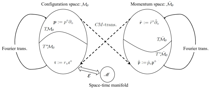
Figure 1: A schematic view of configuration and momentum spaces and transformations among their tangent and co-tangent spaces.

Definition 14.

($CM$-Fourier(–Laplace) transformation)
The $CM$-Fourier transformation and its adjoint transformation are defined as a sequential transformation of Fourier and ${CM}$transformations such that:

$${CF_{\theta}}\hskip 10.00002pt:={C\tilde{M}_{\theta}}{\circ}{FT}:f(r){\mapsto}\hskip 10.00002pt{CF_{\theta}}(f)(\tilde{p}):= \left|{\mathrm{det}\left[\bm{\eta}^{~{}}_{\theta}\right]}\right|\int_{{T^{*}{\mathcal{}M}}_{\theta}}{e^{+i{\eta^{~{}}_{\theta}}^{{\circ\circ}}r_{\circ}\tilde{p}_{\circ}/\hbar}}f(r)\mathfrak{v}_{r},=:\tilde{f}(\tilde{p}),$$ (33a)

$$= \left|{\mathrm{det}\left[\bm{\eta}^{~{}}_{\theta}\right]}\right|\int_{{T^{*}\mathscr{M}}_{\theta}}{e^{+i{\eta^{~{}}_{\theta}}^{{\circ\circ}}r_{\circ}\tilde{p}_{\circ}/\hbar}}f^{~{}}_{{\mathcal{E}}}(x)dx^{0}{\wedge}\cdots{\wedge}dx^{n-1},$$

$${CF_{\theta}}^{-1}:={\tilde{M}C_{\theta}}{\circ}\widetilde{{FT}}:\tilde{f}(\tilde{p}){\mapsto}{CF_{\theta}}^{-1}(\tilde{f})(r):= \frac{\left|{\mathrm{det}\left[\bm{\eta}^{~{}}_{\theta}\right]}\right|}{\left(2\pi\hbar\right)^{n}}\int_{{T^{*}\tilde{{\mathcal{}M}}}_{\theta}}{e^{-i{\eta^{~{}}_{\theta}}^{{\circ\circ}}r_{\circ}\tilde{p}_{\circ}/\hbar}}\tilde{f}(\tilde{p}){{\tilde{\mathfrak{v}}}_{\mathrm{p}}}.$$ (33b)

We note that $\mathfrak{r}\cdot\bm{p}$ and $\tilde{{\bm{r}}}\cdot\tilde{{\mathfrak{p}}}$ are $SO_{n}$ invariant. The Jacobian matrix $\left|{\mathrm{det}\left[\bm{\eta}^{~{}}_{\theta}\right]}\right|$ is unity for any $\theta$; thus, we omit it in formulae, hereafter. In summary, we define the $CM$-Fourier transformation using a two-step approach: the first step is a Fourier transformation within configuration and momentum manifolds, then the second step is the $CM$-transformation between two manifolds, as shown schematically in Figure 1. The configuration manifold is equivalent to the inertial manifold.

Suppose $\psi(x)\in\Omega^{0}({{T^{*}{\mathcal{}M}}_{\theta}})$ is a static wave-function of non-relativistic quantum mechanics and $\hat{\bm{p}}:=\hat{p}^{\circ}\partial_{\circ}\in{V}^{1}({{T{\mathcal{}M}}_{\theta}})$ is a unit vector such that $\left|{\eta^{~{}}_{\theta}}_{{\circ\circ}}\hskip 1.00006pt\hat{p}^{\circ}\hat{p}^{\circ}\right|=1$ and $\hat{p}^{0}=0$. We note that parameter $\theta$ does not appear in this system. Contraction of the wave function concerning the unit vector $\hat{\bm{p}}$ denoted as $\iota^{~{}}_{\hat{\bm{p}}}$ provides

$$\iota^{~{}}_{\hat{\bm{p}}}\psi(\bm{x}):=-\hat{p}^{\circ}\left(\frac{\partial\psi(\bm{x})}{\partial{x}^{\circ}}\right);$$

thus, $\partial_{\circ}\psi$ yields a three-dimensional momentum vector, where a negative sign comes from our convention of the metric tensor and is not essential. In the configuration space, a momentum operator is a differential operator, and a position operator is just a multiplying operator, and vice versa in the momentum space. Our formulation is compatible with a quantum mechanical interpretation.

An alternative way to introduce the Fourier transformation geometrically in physics is to utilize symplectic geometry. We double the inertial manifold as ${{\mathcal{}M}_{\theta}}^{symp}:={{\mathcal{}M}_{\theta}}\oplus{\tilde{{\mathcal{}M}}_{\theta}}$ and introduce the Liouville form and the symplectic form such that:

$${\mathfrak{s}} :={\mathfrak{p}}{\wedge}d\mathfrak{r}\in\Omega^{1}({{T^{*}{\mathcal{}M}}_{\theta}}^{symp})$$

and

$$d{\mathfrak{s}} :=d{\mathfrak{p}}{\wedge}d\mathfrak{r}\in\Omega^{2}({{T^{*}{\mathcal{}M}}_{\theta}}^{symp}).$$

Polarisation is a construction of two $n$-dimensional Hilbert spaces, say $L_{2}({{T^{*}{\mathcal{}M}}_{\theta}})$ and $L_{2}({{T^{*}\tilde{{\mathcal{}M}}}_{\theta}})$, in the $2n$-dimensional space ${{\mathcal{}M}_{\theta}}^{symp}$. In this case, the Fourier transformation is automorphism in ${{\mathcal{}M}_{\theta}}^{symp}$ under a restriction owing to polarization. The inertial manifold is a submanifold of ${{\mathcal{}M}_{\theta}}^{symp}$, and the space-time manifold $\mathscr{M}$ is extended to equip a symplectic structure. The $\theta$-metric tensor is extended to $2n$-dimensional space. This study does not discuss this method more.

At $\theta=0$ and $\theta=1$, an integral kernel of transformations (33a) and (33b) has a pure imaginary exponent; thus, they are Fourier transformation and its inverse. In $\theta\in(0,1)$, an integral kernel has a real exponent, and they are the Fourier–Laplace transformation, which is an analytic continuation of the Fourier transformation. The existence of the inverse transformation is ensured after the appropriate deformation of an integration line. The adjoint transformation (33b) is an inverse Fourier transformation at $\theta=0$ and $\theta=1$; thus, we obtain that

$$\left({CF}_{0}(\tilde{f})(r)\right)^{-1} =\left({CF}_{1}(\tilde{f})(r)\right)^{-1}=f^{~{}}_{\mathcal{E}}(x).$$

For $\theta\in(0,1)$, an integrand of ${CF_{\theta}}(f)(\tilde{p})$ has a real exponent concerning $dt:=dx^{0}$ in ${T^{*}\mathscr{M}}$. We assume the positivity of the energy $E:=\tilde{p}_{0}\geq 0$ owing to physics. Using a complex energy defined as $E_{\theta}:=Ee^{i\pi\theta}$, (33a) and (33b) have representations such that:

$${CF_{\theta}}(f)(\tilde{p}) =\int_{0}^{\infty}{e^{iE_{\theta}t/\hbar}}\hskip 1.99997pt{f}(t,\vec{\tilde{p}})\hskip 1.00006ptdt=:\tilde{f}_{\mathrm{L}}(\tilde{p}),$$ (34a)

$${CF_{\theta}}^{-1}(\tilde{f})(r) ={PV}\int_{\Gamma^{~{}}_{E}}{e^{-iE_{\theta}t/\hbar}}\tilde{f}(E_{\theta},\vec{r})\hskip 1.00006ptdE,$$ (34b)

with

$${f}(t,\vec{\tilde{p}}) :=\int_{T^{*}\mathscr{M}}{e^{+i{\eta^{~{}}_{\theta}}^{{\circ\circ}}r_{\circ}\tilde{p}_{\circ}/\hbar}}f^{~{}}_{\mathcal{E}}(x)\hskip 1.00006ptdx^{1}{\wedge}\cdots{\wedge}dx^{n-1},$$

$$\tilde{f}(E_{\theta},\vec{r}) :=\frac{1}{\left(2\pi\hbar\right)^{n}}\int_{{T^{*}\tilde{{\mathcal{}M}}}_{\theta}}{e^{-i{\eta^{~{}}_{\theta}}^{{\circ\circ}}r_{\circ}\tilde{p}_{\circ}/\hbar}}\tilde{f}_{\mathrm{L}}(\tilde{p})\hskip 1.00006pt\mathfrak{x}^{1}\wedge\cdots\wedge\mathfrak{x}^{n-1},$$

where and $$dE=d\hat{p}^{0} \Gamma^{~{}}_{E} \tilde{f}(E_{\theta},\vec{r}) \vec{\bullet}$$ and is an appropriate integration line in a domain of , where is a three-dimensional space vector.

Remark 15.

(Existence of a Laplace transformation) [22]
Suppose there exists some real constant $c$ for the given $E_{0}\in\mathbb{R}$ such that $|\tilde{f}(E_{\theta},r)|\leq c\hskip 1.99997pte^{-E_{0}t}$ for any $t\geq 0$. Then, the integral (34a) is a holomorphic function on the half-plane $\{E_{\theta}\in\mathbb{C}|\textup{Im}[E_{\theta}]>-\hbar E_{0}\}$. We note that $\textup{Im}[E_{\theta}]=E\sin{(\pi\theta)}>0$ in $\theta\in(0,1)$.

The adjoint transformation (34b) converges with an arbitrary integration-line parallel to the real axis on the abovementioned half-plain and yields ${CF_{\theta}}^{-1}(\tilde{f})(r)=f^{~{}}_{\mathcal{E}}(x)$; thus, it is the inverse Laplace transformation.

IV.2 Green’s function and propagator

We define the Dirac $$\delta$$-distribution in a one-parameter space as

$$\delta(x):= \frac{1}{2\pi}\int_{-\infty}^{\infty}dk\hskip 1.00006pte^{ikx},$$ (35a)

and in an $$n$$-dimensional vector space as

$$\delta^{n}(\bm{x}):= \prod^{n-1}_{j=0}\delta(x_{j}),$$ (35b)

where $$\bm{x}=\{x_{0},\cdots,x_{n-1}\}$$.

Following remarks immediately follow from the definition:

Remark 16.

(Properties of the Dirac $\delta$-distribution)
Suppose $a,b,x\in\mathbb{R}$ and $z\in\mathbb{C}$.

1. For any $\varphi(z){\in}C^{0}(\mathbb{C})$, we have

   $$0\notin[a,b]\implies\int_{a}^{b}\varphi(x)\delta(x)dx=0,$$

   $$0\in[a,b]\implies\int_{a}^{b}\varphi(x)\delta(x)dx=\frac{1}{2\pi i}\oint\frac{\varphi(z)}{z}dz=\varphi(0),$$

   where an integration contour is a clock wise circle around $z=0$.

2. A derivation of the Dirac $\delta$-distribution yields a recurrence formula such that:

   $$x\frac{d^{j}\delta}{dx^{j}}(x)=-j\frac{d^{j-1}\delta}{dx^{j-1}}(x),~{}~{}\textrm{where}~{}~{}1{\leq}j\in\mathbb{Z}.$$

3. Suppose $\bm{F}(\bm{x})=\left(F^{0}(\bm{x}),\cdots,F^{n-1}(\bm{x})\right)\in\mathbb{R}^{n}$ is a holomorphic function with $\bm{F}(\bm{0})=\bm{0}$ and det$[\partial{\bm{F}(\bm{x})}/\partial{\bm{x}}|_{\bm{x}=\bm{0}}]\neq\bm{0}$. Then, we have

   $$\delta\left(\bm{F}(\bm{x})\right)dx^{0}{\wedge}\cdots{\wedge}dx^{n-1} =\textup{det}\left[\frac{\partial{\bm{F}(\bm{x})}}{\partial\bm{x}}\right]^{-1}\delta\left(\bm{x}\right)$$

   $$\times dx^{0}{\wedge}\cdots{\wedge}dx^{n-1}.$$

   Thus, functions in the $\theta$-metric space yields

   $$\delta(\bm{\eta}\bm{x}){{{\sigma^{~{}}_{\theta}}}}dx^{0}{\wedge}\cdots{\wedge}dx^{n-1}=\delta\left(\bm{x}\right){{\mathrm{det}\left[{\mathcal{E}}\right]}}dx^{0}{\wedge}\cdots{\wedge}dx^{n-1}.$$

We consider the Poisson equation (15)^′ for a $p$-form object in the $n$-dimensional $\theta$-metric space; it has a representation using the orthonormal basis (30) such that:

$$\Delta_{\theta}(\bm{x})\mathfrak{F}=\mathfrak{o}$$

$$\implies(-1)^{n(p+1)+1}{\eta^{~{}}_{\theta}}^{{\circ\circ}}\left(\partial_{\circ}\partial_{\circ}F_{\star}\left(\bm{x}\right)\right)\bar{{\mathfrak{h}}}^{\star}=o_{\circ}\left(\bm{x}\right)\bar{{\mathfrak{h}}}^{\circ},$$

where

$$\mathfrak{F}:= F_{\circ}\left(\bm{x}\right){\mathfrak{V}_{\mathrm{p}}}^{\circ}=\sum_{a=1}^{N}F_{a}\left(\bm{x}\right){\mathfrak{V}_{\mathrm{p}}}^{a}$$

and

$$\mathfrak{o}\left(\bm{x}\right) :=o_{\circ}\left(\bm{x}\right)\bar{{\mathfrak{h}}}^{\circ}=\sum_{a=1}^{N-m}o_{a}\left(\bm{x}\right)\bar{{\mathfrak{h}}}^{a}.$$

We note that $\Delta_{\theta}{\mathfrak{V}_{\mathrm{p}}}^{a}=\Delta_{\theta}{\mathfrak{h}}^{a}=0$ for any $a\in\{1,\cdots,m\}$. Green’s function of the Poisson equation is provided using the Dirac $\delta$-distribution. Due to (18)^′, Green’s function for the Dirac $\delta$-distribution is given as

$${G_{\theta}}\left(\delta(\bm{x}){\mathfrak{V}_{\mathrm{p}}}^{a}\right)=\left\{\begin{array}[]{cc}0&\left(1{\leq}a{\leq}m\right),\\ \Delta_{\theta}^{-1}(\bm{x})\delta(\bm{x})\bar{{\mathfrak{h}}}^{a-m}&\left(m+1{\leq}a{\leq}N\right),\end{array}\right.$$

where $\bm{x}:=\{x^{1},\cdots,x^{N-m}\}$ and $a\in\{1,\cdots,N\}$. A formal solution of equation (15)^′ is provided as

$$\mathfrak{F}\left(\bm{x}\right) ={u}_{-1}\left(x_{\circ},\theta\right)\bar{{\mathfrak{h}}}^{\circ}+\int_{D(\bm{y})}d\bm{y}\hskip 1.99997pt{G_{\theta}}\left(\delta(\bm{x}-\bm{y}){\mathfrak{V}_{\mathrm{p}}}^{\circ}\right)o_{\circ}\left(\bm{y}\right),$$

yielding

$$\Delta_{\theta}\left(\bm{x}\right)\mathfrak{F}\left(\bm{x}\right) =\int_{D(\bm{y})}d\bm{y}\hskip 1.99997pt\delta(\bm{x}-\bm{y})\mathfrak{o}\left(\bm{y}\right)=\mathfrak{o}\left(\bm{x}\right),$$

where $d\bm{y}:=dy^{1}{\wedge}\cdots{\wedge}dy^{N-m}$ and $D(\bm{y})$ is a domain of $\bm{y}$ with $D(\bm{x}){\subseteq}D(\bm{y})$.

Example 17.

(The fundamental solution of the Klein–Gordon equation) We consider the Klein–Gordon equation in the four-dimensional $\theta$-metric space with $\theta\in(0,1]$. For scalar function $\phi(\bm{r})\in\Omega^{0}\left({{T^{*}{\mathcal{}M}}_{\theta}}\right)$, the Klein–Gordon equation is provided as

$$\left(\Delta_{\theta}\left(r\right)+\left(\mu/\hbar\right)^{2}\right)\phi(r)= -\frac{1}{\hbar^{2}}f\left(r\right),$$ (36)

where $0<\mu\in\mathbb{R}$ is a real constant, namely a particle mass in physics, and $f(r)$ is a real function. Factor $\hbar^{-2}$ at the right-hand side of (36) is just a convention. In physics, operator $\Delta_{\theta}(r)$ has a physics dimension ${\bm{[}}\Delta_{\theta}(r){\bm{]}}=L^{-2}$, and a particle mass has the energy dimension ${\bm{[}}\mu{\bm{]}}=E$. Though the Planck constant adjusts physical dimensions in formulae, e.g., ${\bm{[}}\Delta_{\theta}(r){\bm{]}}={\bm{[}}\mu^{2}/\hbar^{2}{\bm{]}}=L^{-2}$, the theory is still classical. Scalar function $\phi(r)$ has the energy dimension; thus, $f(\bm{r})$ has $E^{3}$ dimension keeping both sides of (36) to be the same physical dimension of $EL^{-2}$.

Suppose function $\phi(r)$ is the ${C\tilde{M}_{\theta}}$-Fourier–Laplace transformation of $\tilde{\phi}(\tilde{p})\in\Omega^{0}({{T^{*}\tilde{{\mathcal{}M}}}_{\theta}})$ such that:

$$\phi(r):= {C\tilde{M}_{\theta}}\left[\frac{1}{\left(2\pi\hbar\right)^{4}}\int_{{T^{*}\tilde{{\mathcal{}M}}}_{\theta}}{e^{-i{\eta^{~{}}_{\theta}}^{{\circ\circ}}r_{\circ}\tilde{p}_{\circ}/\hbar}}\tilde{\phi}(\tilde{p}){{\tilde{\mathfrak{v}}}_{\mathrm{p}}}\right]$$

$$\in\Omega^{0}\left({{T^{*}{\mathcal{}M}}_{\theta}}\right),$$

yielding

$$\left(\hbar^{2}\Delta_{\theta}(r)+\mu^{2}\right)\phi(r)=\frac{1}{\left(2\pi\hbar\right)^{4}}$$

$$\times{C\tilde{M}_{\theta}}\left[\int_{{T^{*}\tilde{{\mathcal{}M}}}_{\theta}}\left(-{\eta^{~{}}_{\theta}}^{{\circ\circ}}{\tilde{p}_{\circ}}{\tilde{p}_{\circ}}+\mu^{2}\right){e^{-i{\eta^{~{}}_{\theta}}^{{\circ\circ}}r_{\circ}\tilde{p}_{\circ}/\hbar}}\hskip 1.99997pt\tilde{\phi}(\tilde{p}){{\tilde{\mathfrak{v}}}_{\mathrm{p}}}\right].$$

We obtain Green’s function in the configuration space by means of the ${C\tilde{M}_{\theta}}$-Fourier transformation of Green’s function in the momentum space such that:

$${G_{\theta}}\left(\delta^{4}(r)\right) ={C\tilde{M}_{\theta}}\left[\frac{1}{(2\pi\hbar)^{4}}\int_{{T^{*}\tilde{{\mathcal{}M}}}_{\theta}}e^{-i{\eta^{~{}}_{\theta}}^{{\circ\circ}}r_{\circ}\tilde{p}_{\circ}/\hbar}\hskip 1.00006pt{G_{\theta}}(\tilde{p}){{\tilde{\mathfrak{v}}}_{\mathrm{p}}}\right],$$ (37)

where Green’s function in the momentum space is

$${G_{\theta}}(\tilde{p}) :=\left({-{\eta^{~{}}_{\theta}}^{{\circ\circ}}{\tilde{p}_{\circ}}{\tilde{p}_{\circ}}+\mu^{2}}\right)^{-1}\in\Omega^{0}({{T^{*}\tilde{{\mathcal{}M}}}_{\theta}}).$$

We note that integrations (37) is well-defined since ${\eta^{~{}}_{\theta}}^{{\circ\circ}}{\tilde{p}_{\circ}}{\tilde{p}_{\circ}}-\mu^{2}\neq 0$ in $\theta\in(0,1]$. In reality, we obtain from (37) with the definition (35a) that

$$\left(\hbar^{2}\Delta_{\theta}\left(r\right)+\mu^{2}\right){G_{\theta}}\left(\delta^{4}(r)\right)$$

$$={C\tilde{M}_{\theta}}\left[\frac{1}{(2\pi\hbar)^{4}}\int_{{T^{*}\tilde{{\mathcal{}M}}}_{\theta}}{e^{-i{\eta^{~{}}_{\theta}}^{{\circ\circ}}r_{\circ}\tilde{p}_{\circ}/\hbar}}\hskip 1.00006pt{{\tilde{\mathfrak{v}}}_{\mathrm{p}}}\right],$$

$$=\delta^{4}(r)=\delta(t)\delta(x)\delta(y)\delta(z)=\frac{1}{2\pi|\bm{r}|^{2}}\delta(t)\delta^{3}(|\vec{r}|),$$

for $\bm{r}=(t,x,y,z)$. When the metric is quasi-Monkowski as

$$\bm{\eta}^{~{}}_{\theta}\rightarrow\bm{\eta}^{~{}}_{\delta}:=\textup{diag}(1+i\delta^{~{}}_{\theta},-1,-1,-1)+{\mathcal{}O}\left(\delta_{\theta}^{2}\right),~{}\delta^{~{}}_{\theta}>0$$ (38)

with $\exists{c}>0,\delta_{\theta}<c\hskip 1.00006pt|\tilde{p}^{0}|$, Green’s function (37) yields a representation for the metric (38) as

$${G_{F}}\left(t,\vec{r}\right):= \left.{G_{\theta}}\left(\delta(r)\right)\right|_{\theta\rightarrow\delta_{\theta}\rightarrow+0}=\frac{1}{(2\pi\hbar)^{3}}\int\int\int_{-\infty}^{+\infty}d\vec{p}\hskip 1.99997pte^{i\vec{r}\cdot\vec{\tilde{p}}/\hbar}\left(\lim_{\delta_{\theta}\rightarrow+0}\frac{1}{2\pi\hbar}\int_{-\infty}^{+\infty}d\tilde{p}^{0}I_{\tilde{p}^{0}}\right),$$

where

$$I_{\tilde{p}^{0}}:= \frac{{e^{-it\tilde{p}_{0}/\hbar}}{e^{t\tilde{p}_{0}\delta_{\theta}/\hbar}}}{-\tilde{p}^{~{}}_{0}\tilde{p}^{~{}}_{0}+\vec{\tilde{p}}\cdot\vec{\tilde{p}}+\mu^{2}-i\delta_{\theta}},$$

$\vec{\tilde{p}}=\left(\tilde{p}_{1},\tilde{p}_{2},\tilde{p}_{3}\right)$, $\vec{r}=\left(r_{1},r_{2},r_{3}\right)$ and $t:=r_{0}$, and $\vec{\tilde{p}}\cdot\vec{r}$ gives an inner product of two three-dimensional vectors with Euclidean metric. We note that the imaginary part of a denominator is $-i\hskip 1.99997pt\textrm{sign}[(\tilde{p}_{0})^{2}]\delta_{\theta}=-i\delta_{\theta}$. A contour integration after extending $\tilde{p}^{0}$ to a complex variable $\tilde{E}$ as Re$[\tilde{E}]=\tilde{p}^{0}$ provides the $\tilde{p}^{0}$ integral such that:

$$\frac{1}{2\pi\hbar}\int_{-\infty}^{+\infty}d\tilde{p}^{0}I_{\tilde{p}^{0}}=\frac{I_{j}}{2\pi\hbar}\lim_{\rho\rightarrow\infty}\oint_{c^{\rho}_{i}}d\tilde{E}\hskip 1.99997ptI_{\tilde{p}^{0}}$$ (39)

with

$$I_{j}=\left\{\begin{array}[]{lr}-1,&t>0\\ +1,&t<0\end{array},\right.$$

where contour $c^{\rho}_{1}$ ($c^{\rho}_{2}$) is along a real axis with $-\rho<\tilde{E}<\rho$ and a lower (upper) half-circle with a radius of $\rho$, respectively, as shown in Figure 2.

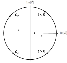
Figure 2: The integration contour of the Feynman propagator. Contour $C_{1}$ ($C_{2}$) is taken to (counter-)clockwise. Two little crosses show a position of poles at $\tilde{E}=\pm\tilde{E}(\vec{\tilde{p}}\hskip 1.99997pt,\delta_{\theta})$.

Straightforward calculations provide

$$\textrm{(\ref{Fint})}= \frac{i\hskip 1.00006pte^{-i\left|t\right|\tilde{E}(\vec{\tilde{p}}\hskip 0.70004pt,\delta_{\theta})/\hbar}}{2\tilde{E}(\vec{\tilde{p}}\hskip 1.00006pt,\delta_{\theta})},$$

where

$$\tilde{E}(\vec{\tilde{p}}\hskip 1.99997pt,\delta_{\theta}):= \sqrt{\vec{\tilde{p}}\cdot\vec{\tilde{p}}+\mu^{2}}-\frac{i\delta_{\theta}}{2\sqrt{\vec{\tilde{p}}\cdot\vec{\tilde{p}}+\mu^{2}}}+{\mathcal{}O}(\delta_{\theta}^{2}).$$

Thus, we obtain Green’s function after taking $\delta_{\theta}\rightarrow+0$ as

$${G_{F}}\left(t,\vec{r}\right):= \frac{i}{(2\pi\hbar)^{3}}\int\int\int_{-\infty}^{+\infty}\frac{d\vec{p}}{2\tilde{E}(\vec{\tilde{p}}\hskip 1.99997pt)}e^{-i\left(\left|t\right|\tilde{E}(\vec{\tilde{p}}\hskip 0.70004pt)-\vec{r}\cdot\vec{\tilde{p}}\right)/\hbar},$$

where $\tilde{E}(\vec{\tilde{p}}\hskip 1.00006pt):=\tilde{E}(\vec{\tilde{p}}\hskip 1.00006pt,0)$; that is referred to as the Feynman propagator in physics. The fundamental solution of the Klein–Gordon equation (36) is provided using the Feynman propagator as

$$\phi(r)= \phi_{0}(r)+\int_{D\left(f(r_{0})\right)}{G_{F}}\left(t-t_{0},\vec{r}-\vec{r}_{0}\right)f(r_{0})\hskip 1.00006ptd^{4}r_{0},$$

where $\phi_{0}(r)$ is a solution of a homogeneous equation such that $\left(\hbar^{2}\Delta_{\theta}(r)+\mu^{2}\right)\phi_{0}(r)=0$.       

We note that the Feynman propagator appears naturally as the propagator in the $\theta$-metric space at the $\theta\rightarrow+0$ limit and is compatible with the causality required from quantum physics.

V Green’s functions of gravity

V.1 Linearised vacuum Einstein-equation

This section discusses Green’s function concerning the Einstein equation. The current author proposed the canonical quantisation of Einstein’s gravity in the previous study[11]. This study provides propagators of spin-connection and vierbein fields. The common understanding of the geometrical gauge theory is that a connection corresponds to a gauge field, and a curvature corresponds to field strength. Moreover, a matter field (a Dirac spinor field) in the Yang–Mills theory corresponds to the vierbein form in general relativity since they are sections in ${T^{*}{\mathcal{}M}}$. Therefore, we apply a gauge-fixing condition on the spin-connection field $\omega$. Although the standard formulation of general relativity does not have a counterpart of a coupling constant in the Yang–Mills theory, this study formulates the $SO_{4}$ covariant differential with the coupling constant ${c^{~{}}_{gr}}$ to discuss two theories in parallel.

The Euler–Lagrange equation of motion owing to the Einstein–Hilbert Lagrangian provides the torsion-less equation and the Einstein equation such that[12]:

$${\mathfrak{T}}^{a} =\left(d{\mathfrak{e}}^{a}+{c^{~{}}_{gr}}\hskip 1.00006pt{\mathfrak{w}}^{a}_{~{}{\circ}}\wedge{\mathfrak{e}}^{\circ}\right)=0,$$ (40a)

and

$$\frac{1}{2}\epsilon_{a{\circ\circ}{\circ}}\mathfrak{R}^{\circ\circ}\wedge{\mathfrak{e}}^{\circ} =\frac{1}{2}\epsilon_{a{\circ\circ}{\circ}}\left(d{\mathfrak{w}}^{\circ\circ}+{c^{~{}}_{gr}}{\mathfrak{w}}^{\circ}_{~{}\star}\wedge{\mathfrak{w}}^{\star{\circ}}\right)\wedge{\mathfrak{e}}^{\circ},$$

$$={\eta^{~{}}_{\theta}}_{a{\circ}}\hskip 1.99997pt{\mathfrak{T}}^{{\circ}},$$ (40b)

where

$${\mathfrak{T}}^{a} =\frac{1}{3!}\left[{\mathfrak{T}}^{a}\right]_{{\circ\circ}{\circ}}{\mathfrak{e}}^{\circ}\wedge{\mathfrak{e}}^{\circ}\wedge{\mathfrak{e}}^{\circ}$$ (40c)

is a stress-energy three-form owing to, e.g., the Yang–Mills matter and gauge fields. We set the cosmological constant to zero for simplicity. A component representation of (40b) in the $$\theta$$-metric space is

$$R^{ab}-\frac{1}{2}R\hskip 1.99997pt{\eta^{~{}}_{\theta}}^{ab} =\mathscr{R}^{{\circ}a}_{\hskip 4.89998pt{\circ}\star}{\eta^{~{}}_{\theta}}^{b\star}-\frac{1}{2}\mathscr{R}^{{\circ}\star}_{\hskip 4.89998pt{\circ}\star}{\eta^{~{}}_{\theta}}^{ab}$$

$$=\frac{1}{2}\left(\frac{1}{3!}\epsilon^{a{\circ\circ}{\circ}}\left[{\mathfrak{T}}^{b}\right]_{{\circ\circ}{\circ}}+(a{\leftrightarrow}b)\right).$$ (40d)

The Bianchi identity (4b) and the torsion-less (40a) in the vacuum immediately gives that

$$\partial_{\circ}\left(R^{a{\circ}}-\frac{1}{2}R\hskip 1.99997pt{\eta^{~{}}_{\theta}}^{a{\circ}}\right) =\partial^{\circ}\mathscr{R}^{a\star}_{\hskip 4.89998pt{\circ}\star}-\frac{1}{2}\partial^{a}\mathscr{R}^{{\circ}\star}_{\hskip 4.89998pt{\circ}\star},$$

$$=0,$$ (41a)

where $$\partial^{a}:={\eta^{~{}}_{\theta}}^{a{\circ}}\partial_{\circ} \mathscr{R}$$. We used anti-symmetry of concerning both pairs of upper and lower indexes. Owing to the definition of the curvature, we obtain an equation for the spin-connection as

$$0= \partial^{\circ}\left(\partial_{\circ}\omega_{\star}^{~{}a\star}-\partial_{\star}\omega_{{\circ}}^{~{}a\star}+{c^{~{}}_{gr}}\left(\omega_{\circ}^{~{}a\bm{\ast}}\omega_{\star}^{~{}\bm{\ast}\star}-\omega_{\star}^{~{}a\bm{\ast}}\omega_{\circ}^{~{}\bm{\ast}\star}\right){\eta^{~{}}_{\theta}}_{\bm{\ast}\bm{\ast}}\right)-\partial^{a}\left(\partial_{\star}\omega_{\circ}^{~{}\star{\circ}}+{c^{~{}}_{gr}}\hskip 1.00006pt\omega_{\circ}^{~{}{\circ}\bm{\ast}}\omega_{\star}^{~{}\bm{\ast}\star}{\eta^{~{}}_{\theta}}_{\bm{\ast}\bm{\ast}}\right)$$

$$= \left(\partial^{\circ}\partial_{\circ}\omega_{\star}^{~{}a\star}-\partial^{\circ}\partial_{\star}\omega_{{\circ}}^{~{}a\star}-\partial^{a}\partial_{\star}\omega_{\circ}^{~{}\star{\circ}}\right)+{c^{~{}}_{gr}}\partial^{\circ}\left(\omega_{\circ}^{~{}a\bm{\ast}}\omega_{\star}^{~{}\bm{\ast}\star}-\omega_{\star}^{~{}a\bm{\ast}}\omega_{\circ}^{~{}\bm{\ast}\star}-\delta^{a}_{\circ}\omega_{\star}^{~{}\star\bm{\ast}}\omega_{\star}^{~{}\bm{\ast}\star}\right){\eta^{~{}}_{\theta}}_{\bm{\ast}\bm{\ast}}.$$ (41b)

In the Yang–Mills theory, one of the standard gauge fixing conditions on a gauge field $A^{\bullet}$ is the covariant gauge such that $\partial_{\mu}A^{\mu}=0$. Together with the massless condition $g_{\mu\nu}A^{\mu}A^{\nu}=0$, two degrees of freedom remain out of four components of the gauge field. We propose a similar gauge condition on the spin-connection as

$$\partial_{\circ}\omega_{b}^{~{}a{\circ}} =0,$$ (42)

which provides $16$ constraints on a total $24$ degrees of freedom in $\omega_{\mu}^{~{}ab}$. In addition, the Einstein equation (40d) provides six constraints (an on-shell condition); thus, two physical degrees of freedom remain in our theory.

The fundamental solution of the equation of motion with a null coupling constant provides a propagator of the free spin-connection field. Then, the perturbation method concerning the coupling constant ${c^{~{}}_{gr}}$ provides a more precise solution to the equation of motion. In reality, an expansion coefficient of a quantum field theoretical scattering matrix is $\alpha_{gr}:={{c^{2}_{gr}}}/4\pi$. For the standard value of ${c^{~{}}_{gr}}=1$, the expansion coefficient for gravity is $\alpha_{gr}\approx 0.0796$, which is smaller than strong interaction ($\alpha_{s}\approx 0.1$), but larger than electromagnetic interaction ($\alpha\approx 0.00730$). Equation (41b) under the free spin-connection field approximation with gauge fixing and massless conditions is the simple Laplace equation such that:

$$\left(\Delta_{\theta}[\bm{\omega}^{0}]_{{\circ}}^{~{}a{\circ}}\right)\left(\xi\in{\mathcal{}M}\right) =0,$$ (43)

$\bm{\omega}^{0}$ is the free spin-connection field fulfilling gauge fixing and massless conditions. The fundamental solution of (43) with quasi-Minkowski metric (38) is

$${G^{a}_{\omega}}(x):=[\bm{\omega}^{0}]_{{\circ}}^{~{}a{\circ}}=\frac{\tilde{\omega}^{a}}{-(\xi^{0})^{2}+(\xi^{1})^{2}+(\xi^{2})^{2}+(\xi^{3})^{2}-i\delta_{\theta}},$$ (44)

owing to (24) for a massless particle ($\mu=0$), where $\tilde{\omega}^{a}$ is a polarization vector of the spin-connection field, which are two independent constant vectors. The spin-connection field is a rank-two massless tensor field corresponding to a spin-two boson.

Next, we consider Green’s function of the vierbein field. The torsion two-form has a component representation in ${T^{*}{\mathcal{}M}}$ and ${T^{*}\mathscr{M}}$ using the standard bases, such as

$${\mathfrak{T}}^{a} =:\frac{1}{2}{\mathcal{T}}^{a}_{\hskip 4.20004pt{\circ\circ}}\hskip 1.99997pt{\mathfrak{e}}^{\circ}\wedge{\mathfrak{e}}^{\circ}=\frac{1}{2}{\mathcal{T}}^{a}_{\hskip 4.20004pt{\circ\circ}}\hskip 1.99997pt{\mathcal{E}}^{\circ}_{\mu}{\mathcal{E}}^{\circ}_{\nu}\hskip 1.99997ptdx^{\mu}{\wedge}dx^{\nu}.$$

Torsion-less equation (40a) is represented using this component representation such as

$${\mathcal{T}}^{a}_{\hskip 4.20004ptbc} =\left(\partial^{~{}}_{\mu}{\mathcal{E}}^{a}_{\nu}-\partial^{~{}}_{\nu}{\mathcal{E}}^{a}_{\mu}+{c^{~{}}_{gr}}\left(\omega_{\mu}^{~{}a{\circ}}{\mathcal{E}}^{\circ}_{\nu}-\omega_{\nu}^{~{}a{\circ}}{\mathcal{E}}^{\circ}_{\mu}\right){\eta^{~{}}_{\theta}}_{{\circ\circ}}\right){\mathcal{E}}_{b}^{\mu}{\mathcal{E}}_{c}^{\nu},$$

$$={\mathcal{E}}^{a}_{\mu}\left(\partial^{~{}}_{c}{\mathcal{E}}_{b}^{\mu}-\partial^{~{}}_{b}{\mathcal{E}}_{c}^{\mu}\right)+{c^{~{}}_{gr}}\left({\omega_{b}^{~{}a}}_{c}-{\omega_{c}^{~{}a}}_{b}\right)=0,$$

where ${\omega_{b}^{~{}a}}_{c}:=\omega_{b}^{~{}a{\circ}}{\eta^{~{}}_{\theta}}_{{\circ}c}$.

Divergence-less concerning an upper index of the torsion form and gauge fixing condition (42) gives constraints such as

$$\partial^{~{}}_{\circ}{\mathcal{T}}^{\circ}_{\hskip 4.20004ptbc} =\partial_{\mu}\left(\partial^{~{}}_{c}{\mathcal{E}}_{b}^{\mu}-\partial^{~{}}_{b}{\mathcal{E}}_{c}^{\mu}\right)+\left(\partial^{~{}}_{c}{\mathcal{E}}_{b}^{\mu}-\partial^{~{}}_{b}{\mathcal{E}}_{c}^{\mu}\right){\mathcal{E}}_{a}^{\nu}\partial_{\nu}{\mathcal{E}}^{a}_{\mu},$$

$$=\partial^{~{}}_{c}\partial^{~{}}_{\mu}{\mathcal{E}}^{\mu}_{b}-\partial^{~{}}_{b}\partial^{~{}}_{\mu}{\mathcal{E}}^{\mu}_{c}-{\mathcal{E}}^{a}_{\nu}\left(\partial^{~{}}_{c}{\mathcal{E}}_{b}^{\nu}-\partial^{~{}}_{b}{\mathcal{E}}_{c}^{\nu}\right)\partial_{\mu}{\mathcal{E}}_{a}^{\mu}.$$

Gauge fixing condition (42) yields constraints equivalent to the de Donder condition on the vierbein such that:

$$\partial^{~{}}_{\circ}{\mathcal{T}}^{\circ}_{\hskip 4.20004ptbc}=0\land(\ref{dwxero})\implies(\partial^{~{}}_{\mu}{\mathcal{E}}^{\mu}_{\bullet})=0.$$ (45)

On the other hand, divergence concerning a lower index provides an equation of motion for the vierbein with the constraint (45) as

$$0 =g_{\theta}^{\hskip 1.39998pt\mu\nu}\partial^{~{}}_{\mu}{\mathcal{T}}^{a}_{\hskip 4.20004pt\nu\rho}$$

$$=\Delta_{\theta}(x){\mathcal{E}}^{a}_{\rho}-g_{\theta}^{\hskip 1.39998pt\mu\nu}\partial^{~{}}_{\rho}\partial^{~{}}_{\mu}{\mathcal{E}}^{a}_{\nu}$$

$$\hskip 51.00014pt+{c^{~{}}_{gr}}\hskip 1.99997ptg_{\theta}^{\hskip 1.39998pt\mu\nu}\partial_{\mu}^{~{}}\left(\omega_{\nu}^{~{}a{\circ}}{\mathcal{E}}^{\circ}_{\rho}-\omega_{\rho}^{~{}a{\circ}}{\mathcal{E}}^{\circ}_{\nu}\right){\eta^{~{}}_{\theta}}_{{\circ\circ}},$$

$$\xrightarrow{~{}{c^{~{}}_{gr}}=0~{}}\Delta_{\theta}(x)\left[{\mathcal{E}}^{0}\right]^{a}_{\nu};$$

thus, an equation of motion under the free vierbein-field approximation is again the simple Laplace equation such that:

$$\left(\Delta_{\theta}\left[{\mathcal{E}}^{0}\right]^{a}_{\nu}\right)(x\in\mathscr{M})=0.$$ (46)

The fundamental solution of (46) with the quasi-Minkowski metric is

$${G^{a}_{{\mathcal{E}}}}(x):=\left[\bm{{\mathcal{E}}}^{0}\right]_{\mu}^{a}=\frac{{{\mathcal{E}}}_{\mu}^{(a)}}{-(x^{0})^{2}+(x^{1})^{2}+(x^{2})^{2}+(x^{3})^{2}-i\delta_{\theta}},$$

where ${{\mathcal{E}}}_{\mu}^{(a)}$ is a polarization vector of the vierbein field. These are components of a spin-one vector defined in ${T\mathscr{M}}$ such that

$${{\mathfrak{e}}}^{(a)}:={{\mathcal{E}}}^{(a)}_{\mu}(x)dx^{\mu},$$

where $a=1,2$ shows two independent polarization vectors. The vierbein field is a massless vector field corresponding to a spin-two boson. Two upper indexes represent tensor components; on the other hand, the lower index points to an inner degree of freedom corresponding to two polarization vectors. We can construct a spin-two polarization state of the metric tensor from the vierbein field using the coupling of angular momenta such as $|2,\pm 2\rangle=|\pm 1\rangle\otimes|\pm 1\rangle$. The spin-connection has no spin-zero state of $|\pm 1,0\rangle$ since it is massless; thus, the metric tensor does not have $|2,\pm 1\rangle$ nor $|2,0\rangle$.

The metric tensor is a symmetric tensor with ten degrees of freedom in four-dimension. On the other hand, ${\mathcal{E}}^{a}_{\mu}$ is not necessarily a symmetric tensor and has 16 degrees of freedom in the four-dimensional space. A local $SO_{4}$ symmetry provides six constraints on the vierbein field; thus, the same number of degrees of freedom as the metric tensor remains in the vierbein field. In addition, four gauge conditions (45) and four torsion-less conditions provide eight additional constraints. Consequently, the vierbein field has two physical degrees of freedom, as we desired.

Example 18.

(A plane wave solution on a flat space-time)
We consider a polarization vector for a plane wave solution in flat space-time. A solution propagating along, e.g., an $x^{1}$-axis, has a polarization tensor such that:

$${{\mathcal{E}}}_{\mu}^{(a)}:=\frac{1}{\sqrt{2}}\left(\begin{array}[]{cccr}1&i&0&0\\ i&1&0&0\\ 0&0&1&1\\ 0&0&1&-1\end{array}\right)$$

$$\implies{g^{~{}}_{\theta}}_{\mu\nu}={\eta^{~{}}_{\theta}}_{\circ\circ}{{\mathcal{E}}}_{\mu}^{({\circ})}{{\mathcal{E}}}_{\nu}^{({\circ})}=\textup{diag}\left(e^{i\pi\theta},-1,-1,-1\right),$$

with a circular polarization. This polarization vector yields a polarization vector of the spin-connection field such that:

$$\omega^{(a)}=\frac{1}{\sqrt{2}}\left(0,0,\omega_{2}^{~{}23}-\omega_{3}^{~{}23},-\omega_{2}^{~{}23}-\omega_{3}^{~{}23}\right).$$

We note that states with two polarization vectors,

$${\mathfrak{e}}^{(\lambda=\bm{+})} :={{\mathcal{E}}}_{\mu}^{(2)}dx^{\mu}=\frac{1}{\sqrt{2}}\left(dx^{2}+dx^{3}\right)$$

and

$${\mathfrak{e}}^{(\lambda=\bm{\times})} :={{\mathcal{E}}}_{\mu}^{(3)}dx^{\mu}=\frac{1}{\sqrt{2}}\left(dx^{2}-dx^{3}\right),$$

have a dynamic degree and are physically observable in the quantum field theory, similar to the polarization vector of photon in QED. The upper index of the vierbein corresponds to an index to specify two transverse, one longitudinal and one scalar photons of the photon polarization vector. On the other hand, two polarization vectors of the spin-connection field have no counterparts in QED and are two independent vector functions:

$${\mathfrak{w}}^{(\lambda=1)} :=\omega_{2}^{(1)}\hskip 1.00006pt{\mathfrak{e}}^{2}=\omega_{\mu}^{(1)}[{\mathcal{E}}^{-1}]^{\mu}_{2}\hskip 1.00006ptdx^{2}=\omega^{(1)}dx^{2}$$

and

$${\mathfrak{w}}^{(\lambda=2)} :=\omega_{3}^{(2)}\hskip 1.00006pt{\mathfrak{e}}^{3}=\omega_{\mu}^{(2)}[{\mathcal{E}}^{-1}]^{\mu}_{3}\hskip 1.00006ptdx^{3}=\omega^{(2)}dx^{3},$$

where

$$\omega^{(1)} :=\frac{1}{{\sqrt{2}}}\left(\omega_{2}^{(1)}+\omega_{3}^{(1)}\right)$$

and

$$\omega^{(2)} :=\frac{1}{{\sqrt{2}}}\left(\omega_{2}^{(2)}+\omega_{3}^{(2)}\right).$$

Consequently, we obtain Green’s functions in the momentum space such that

$${\hat{G}^{(\lambda)}_{\mathcal{E}}}(\tilde{p}) :=\frac{\tilde{\mathcal{E}}_{a}^{(\lambda)}}{-\tilde{p}^{~{}}_{0}\tilde{p}^{~{}}_{0}+\vec{\tilde{p}}\cdot\vec{\tilde{p}}-i\delta_{\theta}},\hskip 20.00003pt\lambda=(\bm{+},\bm{\times}),$$

and

$$\hat{G}^{(\lambda)}_{\omega}(\tilde{p}) :=\frac{\tilde{\omega}^{(\lambda)}}{-\tilde{p}^{~{}}_{0}\tilde{p}^{~{}}_{0}+\vec{\tilde{p}}\cdot\vec{\tilde{p}}-i\delta_{\theta}},\hskip 20.00003pt\lambda=(1,2),$$

in the quasi-Minkowski metric. Polarization vectors $\tilde{\mathcal{E}}_{a}^{(\lambda)}$ are components of the vector defined in ${{T^{*}\tilde{{\mathcal{}M}}}_{\theta}}$ such that:

$$\tilde{\mathfrak{e}}^{+} =\tilde{{\mathcal{E}}}_{{\circ}}^{(+)}\hskip 1.00006ptd\tilde{p}^{\circ}=\frac{1}{\sqrt{2}}\tilde{{\mathcal{E}}}(\tilde{p})\left(d\tilde{p}^{2}+d\tilde{p}^{3}\right)$$

and

$$\tilde{\mathfrak{e}}^{\times} =\tilde{{\mathcal{E}}}_{{\circ}}^{(\times)}\hskip 1.00006ptd\tilde{p}^{\circ}=\frac{1}{\sqrt{2}}\tilde{{\mathcal{E}}}(\tilde{p})\left(d\tilde{p}^{2}-d\tilde{p}^{3}\right),$$

where $\tilde{{\mathcal{E}}}$ is the $CM$-Fourier transformation of unity. Similarly, $\tilde{\omega}^{(\lambda)}(\tilde{p})$ are given as the $CM$-Fourier transformation of $\omega^{(\lambda)}(x)$. As a result, $\hat{G}^{(\lambda)}_{\bullet}$ are Green’s functions in a momentum space as a distribution[21].       

V.2 Green’s function due to exact solutions

This section treats vierbein and spin-connection fields as classical external fields in the quantum field theory. In the Yang–Mills theory with $SU(N)$ gauge group in curved space-time, a classical equation of motion of spinor field $\psi$ is

$$~{}\hbar\left(i\gamma^{\circ}\partial_{\circ}-\frac{1}{2}{c^{~{}}_{gr}}\hskip 1.00006pt\gamma^{\circ}{\mathcal{E}}_{\circ}^{\mu}\omega_{\mu}^{~{}{\star\star}}{S}_{\star\star}+{ic^{~{}}_{SU}}\hskip 1.00006pt\gamma^{\circ}{\mathscr{A}}^{I}_{\circ}t_{I}\right)\psi={\mu}\hskip 1.00006pt\psi,$$

where ${\mathscr{A}}^{I}_{a}$ are spin-connections of the gauge field with coupling constant ${c^{~{}}_{SU}}$, $\mu$ is a mass of the spinor field, $\gamma^{\bullet}$ are Dirac matrices, $S^{\bullet\bullet}$ are generators of a $spin(1,3)$ group represented as $S^{ab}:=i[\gamma^{a},\gamma^{b}]/4$ using the trivial basis, and $t_{I}$ is the fundamental representation of gauge group. We note that all fields $\psi$, ${\mathcal{E}}\omega$, ${\mathscr{A}}$ and differential operator $\partial_{a}=\partial/\partial{\xi^{a}}$ are defined in ${{\mathcal{}M}_{\theta}}$. A definition of the Dirac gamma matrices in the $\theta$-metric space is given in Ref.[12]. In the quantum field theory, the standard perturbation calculation method (Feynman-diagram method) treats all fields in the momentum space. We can utilize the standard method of the quantum Yang–Mills theory in classical curved space-time when we have vierbein and spin-connection fields as exact solutions of the Einstein equation in the momentum space.

In a semi-classical theory with a gravitational background, the quantum field theory treats a gravitational field as a classical external field using the exact solution of the Einstein equation. Vierbein and spin-connection fields in a configuration space are Fourier-transformed to Green’s function in momentum space and interact with quantum matter and gauge fields. We consider Green’s functions of vierbein and spin-connection fields of the Schwarzschild solution:

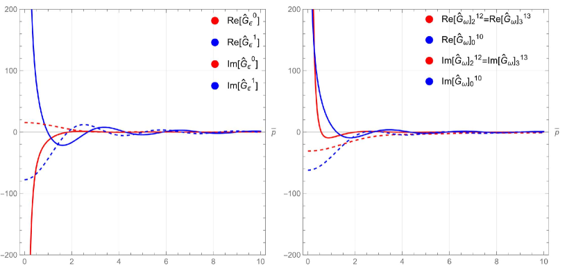
Figure 3: Green’s functions of the vierbein (left) and the spin-connection (right) in the momentum space for the Schwarzschild solution as a function of $\bar{p}$. Numerical values are normalised by a factor $(2\pi\hbar)^{2}$ with $2{R_{\text{S}}}=\delta{E}=1$.

Example 19.

(Schwarzschild solution) The vierbein forms of the Schwarzschild solution using polar-coordinate $d\rho^{\mu}=(dt,dr,d\vartheta,d\varphi)$ in ${{T^{*}{\mathcal{}M}}_{\theta}}$ are

$${\mathfrak{e}}^{a}={\mathcal{E}}^{a}_{\mu}\hskip 1.00006ptdx^{\mu},$$

where

$$\left\{\begin{array}[]{clcl}{\mathfrak{e}}^{0}&=f_{\textrm{S}}(r)\hskip 1.00006ptdt,&{\mathfrak{e}}^{1}&=f_{\textrm{S}}(r)^{-1}\hskip 1.00006ptdr,\\ {\mathfrak{e}}^{2}&=r\hskip 1.00006ptd\vartheta,&{\mathfrak{e}}^{3}&=r\sin{\vartheta}\hskip 1.00006ptd\varphi,\end{array}\right.$$ (47c)

and

$$f_{\textrm{S}}(r):=\sqrt{1-\frac{{R_{\text{S}}}}{r}},~{}~{}~{}{R_{\text{S}}}:=\frac{\kappa M}{4\pi},$$ (47d)

where $${R_{\text{S}}}$$ is the Schwarzschild radius.

Vierbein matrices providing vierbein forms (47c) in the $\theta$-metric space are

$${\mathcal{E}}^{a}_{\mu}{dx^{\mu}} =[{\mathcal{E}}_{\textrm{Schw}}]^{a}_{\circ}[{\mathcal{E}}_{pol}]^{\circ}_{\mu}{dx^{\mu}}$$

$$=\left(\begin{array}[]{cccc}f_{\textrm{S}}(r)&0&0&~{}0\\ 0&f_{\textrm{S}}(r)^{-1}&0&~{}0\\ 0&0&1&~{}0\\ 0&0&0&~{}1\end{array}\right)\left(\begin{array}[]{crrr}e^{i\pi\theta}&0{}{}{}{}&0{}{}{}{}&0{}{}\\ 0&\cos{\varphi}\sin{\vartheta}&\sin{\varphi}\sin{\vartheta}&\cos{\vartheta}\\ 0&r\cos{\varphi}\cos{\vartheta}&r\sin{\varphi}\cos{\vartheta}&-r\sin{\vartheta}\\ 0&-r\sin{\varphi}\sin{\vartheta}&r\cos{\varphi}\sin{\vartheta}&0{}{}\end{array}\right)\left(\begin{array}[]{c}dt\\ dx\\ dy\\ dz\end{array}\right).$$

We consider Green’s function of the vierbein ${\mathcal{E}}_{\mu}^{a}(x)$: a $CM$-Fourier transformation of Green’s function in the configuration space provides that in the momentum space. Green’s function with the coordinate vector $dp^{a}=\left(dE,dp,d\vartheta,d\varphi\right)$ is

$$\hat{G}^{a}_{\mathcal{E}}(E_{p},|\vec{\tilde{p}}|)= \int_{-\infty}^{\infty}dt\hskip 1.00006pte^{i(E_{p}+i\delta_{\theta})|t|/\hbar}\int_{0}^{2\pi}d\varphi\int_{-1}^{1}d\cos{\vartheta}\int_{0}^{\infty}dr\hskip 1.99997pte^{-i\vec{r}\cdot\vec{\tilde{p}}/\hbar}\hskip 5.0ptr^{2}\left(f_{\textrm{S}}(r),f_{\textrm{S}}(r)^{-1},1,1\right),$$

where $\vec{r}\cdot\vec{p}=p\hskip 1.99997ptr\cos{\vartheta}$, $(\exists{c}>0,0<\delta_{\theta}<c\hskip 1.00006ptE_{p})$ and $E_{p}>0$ is an energy of a graviton. We obtain Green’s functions of the vierbeins after the Fourier transformation as

$$\frac{\hat{G}^{0}_{\mathcal{E}}\left(E_{p},\bar{p}\right)}{2\pi\hbar} =\frac{{\pi^{2}{R_{\text{S}}}^{3}}}{4}\left(\frac{-\cos{\bar{p}}\hskip 1.99997ptJ_{1}\left(\bar{p}\right)+\sin{\bar{p}}\hskip 1.99997ptY_{1}\left(\bar{p}\right)}{\bar{p}^{2}}-2i\frac{\sin{\hskip 1.00006pt\bar{p}}\hskip 1.99997ptJ_{1}\left(\bar{p}\right)}{\bar{p}^{2}}\right)\hskip 1.00006pt\delta E_{p},$$

$$\simeq-\frac{\pi{R_{\text{S}}}^{3}}{2}\left(\frac{1}{\bar{p}^{2}}+\frac{\pi}{4\bar{p}}-\frac{1}{2}\left(\log{\frac{\bar{p}}{2}}-\frac{1}{6}+\gamma^{~{}}_{E}+i\pi\right)+{\mathcal{}O}\left(\bar{p}^{1}\right)\right)\hskip 1.00006pt\delta E_{p},$$

$$\frac{\hat{G}^{1}_{\mathcal{E}}\left(E_{p},\bar{p}\right)}{2\pi\hbar} =\frac{\pi^{2}{R_{\text{S}}}^{3}}{4}\left\{\cos{\bar{p}}\hskip 1.00006pt\left(2\frac{J_{0}(\bar{p})+Y_{1}(\bar{p})}{\bar{p}}-\frac{J_{1}(\bar{p})}{\bar{p}^{2}}\right)-\sin{\bar{p}}\left(2\frac{J_{1}(\bar{p})+Y_{0}(\bar{p})}{\bar{p}}-\frac{Y_{1}(\bar{p})}{\bar{p}^{2}}\right)\right.$$

$$\left.\hskip 10.00002pt+2i\left(\sin{\bar{p}}\left(\frac{J_{1}(\bar{p})}{\bar{p}^{2}}-\frac{2J_{0}(\bar{p})}{\bar{p}}\right)-\cos{\bar{p}}\hskip 1.00006pt\hskip 1.99997pt\frac{2J_{1}(\bar{p})}{\bar{p}}\right)\right\}\hskip 1.00006pt\delta E_{p},$$

$$\simeq\frac{\pi{R_{\text{S}}}^{3}}{2}\left(\frac{1}{\bar{p}^{2}}+\frac{3\pi}{4\bar{p}}-\frac{5}{2}\left(\log{\frac{\bar{p}}{2}}+\gamma^{~{}}_{E}-+i\pi+\frac{7}{30}\right)+{\mathcal{}O}\left(\bar{p}^{1}\right)\right)\hskip 1.00006pt\delta E_{p},,$$

$$\frac{\hat{G}^{2}_{\mathcal{E}}\left(E_{p},\bar{p}\right)}{2\pi\hbar} =\frac{\hat{G}^{3}_{\mathcal{E}}\left(E_{p},\bar{p}\right)}{2\pi\hbar}=\pi\hbar\hskip 1.99997pt\delta^{2}{E\bar{p}},$$

where

$$\bar{p} :=\frac{{{R_{\text{S}}}}}{2\hbar}|\vec{\tilde{p}}|,~{}~{}\delta^{2}{E\bar{p}}=2\pi\hbar^{2}\frac{\delta(|\vec{\tilde{p}}|)}{|\vec{\tilde{p}}|^{2}}\delta{E_{p}}=\frac{\pi{R_{\text{S}}}^{3}}{4\hbar}\frac{\delta(\bar{p})}{\bar{p}^{2}}\delta{E_{p}},~{}~{}\delta{E_{p}}:=\left.\hskip 1.00006pt\delta(E_{p}+i\delta_{\theta})\right|_{\delta_{\theta}\rightarrow 0},$$

$\gamma^{~{}}_{E}$ is a Euler’s constant. $J_{i}(\bullet)$ and $Y_{i}(\bullet)$ $(i=1,2)$ are Bessel functions of the first and the second kind, respectively. We note that $\bar{p}$ is dimensionless momentum variable.

Corresponding spin-connection forms $[\omega{\mathcal{E}}]_{c}^{~{}ab}:={c^{~{}}_{gr}}\hskip 1.99997pt\omega_{\mu}^{~{}ab}[{\mathcal{E}}^{-1}]^{\mu}_{c}$ are

$$[\omega{\mathcal{E}}]^{~{}01}_{0} =-[\omega{\mathcal{E}}]^{~{}10}_{0}=-\frac{{{R_{\text{S}}}}}{2f_{\textrm{S}}(r)r^{2}},\hskip 20.00003pt[\omega{\mathcal{E}}]^{~{}12}_{2}=-[\omega{\mathcal{E}}]^{~{}21}_{2}=\frac{f_{\textrm{S}}(r)}{r},$$

$$[\omega{\mathcal{E}}]^{~{}13}_{3} =-[\omega{\mathcal{E}}]^{~{}31}_{3}=\frac{f_{\textrm{S}}(r)}{r},\hskip 28.99997pt[\omega{\mathcal{E}}]^{~{}23}_{3}=-[\omega{\mathcal{E}}]^{~{}32}_{3}=\frac{\cos\vartheta}{r\sin{\vartheta}},$$

and otherwise zero.

A Fourier transformation provides Green’s function in the momentum space such that:

$$\frac{\left[\hat{G}_{\omega}(E_{p},\bar{p})\right]^{~{}10}_{0}}{2\pi\hbar} =-\frac{\pi^{2}{R_{\text{S}}}^{2}}{2}\frac{\sin{\bar{p}}\hskip 1.99997ptY_{0}(\bar{p})-\left(\cos{\bar{p}}\hskip 1.00006pt-2i\sin{\bar{p}}\right)J_{0}(\bar{p})}{\bar{p}}\hskip 1.00006pt\delta E_{p},$$

$$\simeq\frac{\pi{R_{\text{S}}}^{2}}{2}\left(\frac{\pi}{\bar{p}}-2\left(\log{\frac{\bar{p}}{2}}+\gamma^{~{}}_{E}+i\pi\right)+{\mathcal{}O}\left(\bar{p}^{1}\right)\right)\hskip 1.00006pt\delta E_{p},$$

$$\frac{\left[\hat{G}_{\omega}(E_{p},\bar{p})\right]^{~{}12}_{2}}{2\pi\hbar} =\frac{\left[\hat{G}_{\omega}(E_{p},\bar{p})\right]^{~{}13}_{3}}{2\pi\hbar},$$

$$=\frac{\pi^{2}{R_{\text{S}}}^{2}}{2}\frac{\sin{\bar{p}}\left(Y_{0}(\bar{p})-J_{1}(\bar{p})-2iJ_{0}(\bar{p})\right)-\cos{\bar{p}}\hskip 1.00006pt\left(Y_{1}(\bar{p})+J_{0}(\bar{p})-2iJ_{1}(\bar{p})\right)}{\bar{p}}\hskip 1.00006pt\delta E_{p},$$

$$\simeq\frac{\pi{R_{\text{S}}}^{2}}{2}\left(\frac{2}{\bar{p}^{2}}-\frac{\pi}{\bar{p}}+\log{\frac{\bar{p}}{2}}+\gamma^{~{}}_{E}-\frac{1}{2}-i\pi+{\mathcal{}O}\left(\bar{p}^{1}\right)\right)\hskip 1.00006pt\delta E_{p},$$

$$\frac{\left[\hat{G}_{\omega}(E_{p},\bar{p})\right]^{~{}23}_{3}}{2\pi\hbar} =0.$$

A behavior of Green’s functions with $\delta{E}=1$ are drawn in Figure 3. An asymptotic behavior of Green’s functions is $\hat{G}_{{\mathcal{E}}}(1,\infty)=\hat{G}_{\omega}(1,\infty)=0$.       

VI Summary

The author proposed a non-perturbative canonical quantisation of general relativity in the Heisenberg picture in the previous work[11]. For concrete quantum mechanical calculations of gravitational phenomena, we need a perturbative expansion of physical processes, such as scattering processes concerning gravitons. This report provides wave functions and Green’s functions (propagators) of gravitational fields of the vierbein and the spin-connection fields. They are essential ingredients of perturbed calculations using the diagrammatic method. The existence of Green’s function for the Laplace–Beltrami operator in curved space and with an indefinite metric is ensured owing to the Hodge harmonic analysis extended to the $\theta$-metric space. The analyticity of Green’s function is naturally fixed by the $\theta$-metric consistent with keeping a causality as expected from physics.

The standard method of a perturbative quantum field theory in a flat Minkowski space utilizes the momentum space for calculations; the momentum space consists of vectors Fourier transferred from the configurations space. An integration kernel of the Fourier transformation is a solution of the wave equation; thus, the Fourier transformation corresponds to an expansion of solutions of the exact (interacting) non-linear equation of motion by the fundamental solutions of free (non-interacting) fields. In curved space-time, the physical interpretation of the momentum space is not straightforward, especially for gravitational fields of the vierbein and spin-connection forms. We note that the general relativity standard linearization method with the weak-field approximation differs from that in the quantum Yang-Mills theory.

This report proposed a novel definition of the momentum space in curved space-time. A vector in the configuration space is transferred to that in the momentum space through two steps, the Fourier(-Laplace)-transformation and the $CM$ transformation. The spin-connection field owns the information on the curved space-time in the configuration space. The $CM$-Fourier(–Laplace) transformed vierbein, and spin-connection fields are defined in the momentum space with the flat metric. This report also proposed the linearisation of the Einstein equation as a free field consistent with that for the Yang–Mills gauge field. The proposed linearisation does not utilize the weak-field approximation; thus, the method is applicable for highly caved space-time.

We gave two examples of Green’s function of gravitational fields, the plane wave solution and the Schwarzschild solution. After the perturbative quantisation of gravitational fields, we can calculate the gravitational effects using the diagrammatic method to the quantum Yang–Mills theory owing to Green’s functions in this report. E.g., the Hawking radiation from black holes and a gravitational correction of the muon (and also electron) anomalous magnetic moment are the possible candidates for an application.