Characterizing Different Motility Induced Regimes in Active Matter with Machine Learning and Noise

Abstract

We examine motility-induced phase separation (MIPS) in two-dimensional run and tumble disk systems using both machine learning and noise fluctuation analysis. Our measures suggest that within the MIPS state there are several distinct regimes as a function of density and run time, so that systems with MIPS transitions exhibit an active fluid, an active crystal, and a critical regime. The different regimes can be detected by combining an order parameter extracted from principal component analysis with a cluster stability measurement. The principal component-derived order parameter is maximized in the critical regime, remains low in the active fluid, and has an intermediate value in the active crystal regime. We demonstrate that machine learning can better capture dynamical properties of the MIPS regimes compared to more standard structural measures such as the maximum cluster size. The different regimes can also be characterized via changes in the noise power of the fluctuations in the average speed. In the critical regime, the noise power passes through a maximum and has a broad spectrum with a $1/f^{1.6}$ signature, similar to the noise observed near depinning transitions or for solids undergoing plastic deformation.

I Introduction

Active matter denotes systems composed of self-propelling agents or particles that move using internal driving or energy harvested from the surrounding environment Ramaswamy (2010); Marchetti et al. (2013); Bechinger et al. (2016). Examples of active matter include bacteria Sokolov and Aranson (2012), engineered systems such as robots Scholz et al. (2018), and colloidal particles that move using a variety of mechanisms Palacci et al. (2013); Wang et al. (2015); Bechinger et al. (2016) such as light Buttinoni et al. (2013); Schmidt et al. (2019) or magnets Demirörs et al. (2018). One of the most studied phenomena found in models of interacting active particles, such as active disks, is motility-induced phase segregation (MIPS), which occurs even for systems with only repulsive interactions when the persistence of the motion is large enough. In MIPS, for densities well below those at which the system can uniformly crystallize, the system phase-separates into a dense or crystalline phase coexisting with a low density gas Fily and Marchetti (2012). Although MIPS has generally been regarded as a single phase Redner et al. (2013); Palacci et al. (2013); Buttinoni et al. (2013); Cates and Tailleur (2015), its intrinsically dynamic nature means that there could be different dynamic regimes or changing structures within the MIPS state.

Various studies have noted interruptions to MIPS due to mechanisms such as polar alignment between neighboring particles van der Linden et al. (2019), inertia Dai et al. (2020), or large-scale shear motions due to the high speed of individual particles Kichatov et al. (2021). Work on low-density, apolar active matter has shown the cluster size and average speed of active colloids exhibit power law distributions Ginot et al. (2018). Experiments have revealed a variety of phases in suspensions of bacteria Sokolov and Aranson (2012) and run-and-tumble Quincke rollers Karani et al. (2019), though in these systems the hydrodynamics of the suspending fluids may play a role. Furthermore, torque can mediate an active clustered phase distinct from MIPS  Zhang et al. (2021). In very dense active matter, different kinds of intermittency have been found as a function of activity when the system is a solid Mandal et al. (2020).

To characterize MIPS, a number of traditional measurements are commonly used that have been adapted from equilibrium systems, such as average cluster size, the radial distribution function, or the amount of bond orientational order Steinhardt et al. (1983). Such measures were designed to distinguish a variety of transitions including short versus long-range order or order-order structural phase transitions; however, these measures may fail to detect notable features due to dynamic changes or the fluctuating inhomogeneity of particle environments. As a result, the measures may give the same signal for states where distinct types of dynamical motion is occurring if the static structures in these states are sufficiently similar.

Machine learning (ML) is being employed to an increasing extent as a method for characterizing active matter Martiniani et al. (2019); Cichos et al. (2020). In some ML approaches, a variety of factors are combined into a single optimized order parameter, $P_{1}$, that can make it possible to identify different dynamics in strongly nonequilibrium systems. In previous work, machine learning has been used to discern phases in soft non-active granular disks and a variety of equilibrium Jadrich et al. (2018a) and nonequilibrium systems Jadrich et al. (2018b), as well as to find transitions between different dynamical nonequilibrium phases in driven systems McDermott et al. (2020).

Another frequently used characterization method for nonequilibrium driven systems is measuring features in noise fluctuations Weissman (1988); Sethna et al. (2001), such as the Barkhausen noise in driven magnetic systems Durin and Zapperi (2005). Similar measures have been applied to sliding charge density waves Grüner (1988), the depinning of superconducting vortices Marley et al. (1995); Field et al. (1995); Olson et al. (1998); Okuma et al. (2008), driven systems with quenched disorder Reichhardt and Reichhardt (2017), and glass transitions in electron systems Jaroszyński et al. (2002); Reichhardt and Olson Reichhardt (2004). The power spectrum constructed from a time series of some fluctuating quantity can show transitions from a narrow band signature, indicative of the presence of a characteristic frequency, to broad band or $1/f^{\alpha}$ noise characteristics, where the exponent $\alpha$ can range from $\alpha=0$, associated with white noise, to values as large as $\alpha=2.0$ in many systems. The noise power, $S_{0}$, obtained by integrating the power spectrum over a particular frequency window Rabin et al. (1998), often peaks when the system goes through an equilibrium Chen and Yu (2007) or nonequilibrium Olson et al. (1998); Okuma et al. (2008) phase transition. In the case of crackling noise, there can be a disorder-induced critical point at which the system exhibits a broad distribution of avalanche sizes as well as power law fluctuation spectra Kuntz and Sethna (2000); Travesset et al. (2002), and in some cases, noise measurements can be used to identify the universality class of the underlying phase transition. Despite the widespread use of noise measures to characterize collective dynamics in condensed matter systems, noise analysis has not been applied systematically to active matter. Much of the microscopic dynamics in active matter systems can be accessed directly in both simulations and experiments, so time series of a variety of quantities should readily be available in many of these systems.

Here we perform numerical simulations of two-dimensional systems of run-and-tumble active disks at varied densities and persistence lengths both inside and outside of the MIPS state, and show that unsupervised machine learning and noise analysis can be used to identify distinct dynamical regimes within MIPS. We show that ML is better able to characterize dynamical behaviors in the MIPS state than traditional clustering measures. Based on our ML and noise analysis, we propose that there are three regimes in systems that exhibit MIPS behavior. In the active fluid or non-MIPS regime where there is no clustering, the ML principal component $P_{1}$ and the noise power $S_{0}$ are both low. In the active crystal regime found for high persistence lengths and high densities, the system has large-scale crystalline order and both $P_{1}$ and $S_{0}$ have intermediate values. Finally, in the critical regime at intermediate persistence lengths and intermediate densities, both $P_{1}$ and $S_{0}$ are large. The principal component-derived order parameter $P_{1}$ passes through its maximum value in the critical regime, and at the same time we observe the largest velocity noise power $S_{0}$ along with broadband spectra of the form $1/f^{1.62}$. Both $P_{1}$ and $S_{0}$ have nonmonotonic signatures and, after reaching maximum values, decrease as either the density or the persistence length is increased. For intermediate densities, the cluster stability measure also peaks in the same persistence length region as the peaks in $P_{1}$ and $S_{0}$ before decreasing again at higher persistence lengths. The dynamics in the critical regime resemble those of systems exhibiting plastic depinning, which also show a peak in the noise power and similar $1/f^{\alpha}$ noise signatures. At higher densities, the values of both the noise power and the first principal component-derived order parameter are reduced.

II Simulation and System

We model the active particles as $N_{d}$ disks interacting via excluded volume with no polar alignment. The disks are confined in a two-dimensional (2D) system of size $L\times L$ with side length $L=60.0$ and with periodic boundary conditions in the $x$ and $y$ directions. Each disk has a fixed radius of $r_{d}=0.5$. The disk positions are initialized at randomly chosen non-overlapping locations, and the system is allowed to evolve until it reaches steady state behavior. We vary the packing fraction or area density of the disks $\phi=\pi r_{d}^{2}N_{d}/L^{2}$ by changing N_d while holding the disk radius and sample size fixed. For most of the results presented here, we work at densities $\phi$ that are well below the jamming density $\phi_{J}\approx 0.9$ of monodisperse passive disks Reichhardt and Reichhardt (2014).

Each disk self-propels under an active force $\vec{F}_{i}^{a}$ and runs in a randomly chosen constant direction ${\bf{\hat{m}}}_{i}$ for $\tau$ simulation time steps, where $\tau$ is the persistence time, before performing an instantaneous tumble and selecting a new randomly chosen direction. We fix the magnitude of the active force to $F^{a}=1.0$ for each disk and initialize the clock of each particle, which tracks the amount of time since the last tumble, to random values in the range $[0,\tau]$ so that individual disks tumble at randomly distributed times. In the absence of other interactions, a disk would travel a distance $r_{l}=F^{a}\tau\Delta t$ during a single run interval, where the simulation time step is $\Delta t=0.002$.

Disk-disk interactions are modeled by a short range harmonic repulsive force

$$\vec{F}_{ij}^{dd}=k_{d}(\vec{r}_{i}-\vec{r}_{j})\Theta(|\vec{r}_{i}-\vec{r_{j}}|-2r_{d})$$ (1)

for disks with positions $\vec{r}_{i}$ and $\vec{r}_{j}$, where the spring constant $k_{d}=50$ and $\Theta$ is the Heaviside step function. The overdamped equation of motion for an individual disk $i$ is

$$\eta\vec{v}_{i}=\vec{F}_{i}^{a}+\sum_{i\neq j}^{N_{d}}\vec{F}_{ij}.$$ (2)

where $\eta=1$ is the damping constant representing the viscosity of the implicit suspending liquid. We integrate the equations of motion with a standard Verlet algorithm.

III Principal Component Analysis of Disk Systems

For the machine learning, we employ principal component analysis (PCA) Abdi and Williams (2010), which calculates directions of maximum variance in a data set comprised of $M$ samples of $N$ measurements. PCA can identify patterns in large data sets and perform dimensionality reduction tasks. In condensed matter applications, it has been shown that an order parameter derived from PCA can be used to identify phase transitions in on-lattice, Ising spin type systems by operating directly with matrices describing spin states  Carrasquilla and Melko (2017); Hu et al. (2017). To perform PCA on off-lattice systems of interacting disks, we construct matrices containing the instantaneous interparticle distances, $r_{ij}=|{\vec{r}}_{i}-{\vec{r}}_{j}|$. The measurement is described in detail in Refs. Jadrich et al. (2018a); McDermott et al. (2020). The distance matrices are calculated for a subset of probe particles rather than for all particles in the system, and it is important to sort the interparticle distances in order to construct the feature vector $\vec{f}_{i}$ for each probe particle $i$:

$$\vec{f}_{i}=[r_{i0},r_{i1},r_{i2},...,r_{ij},...,r_{in}].$$ (3)

with $r_{i0}<r_{i1}<...<r_{in}$. It is necessary to prewhiten the feature vector based upon a PCA analysis of an ideal gas, giving a whitened feature factor $\vec{f}^{w}_{i}=\vec{W_{0}}\vec{f}_{i}$. The principal components are then calculated according to

$$\vec{p}_{i}=\vec{W}\vec{f}^{w}_{i}.$$ (4)

The machine learning derived order parameter $P_{1}$ is defined as the normalized average of the absolute value of the first entry of the principal component vector

$$P_{1}=\langle|p_{1}|\rangle/\sqrt{\lambda_{1}},$$ (5)

where $\lambda_{1}$ is the eigenvalue associated with the first principal component. PCA performs best when the variance is high, so we analyze feature matrices constructed with data from multiple timesteps that span all possible transitions in the system. For example, we calculate the features every 1000 simulation timesteps during a period of 10⁶ simulation steps in order to permit comparison between early (transient) and late (steady state) phenomena.

In addition to PCA, we apply several other measures to our system. To separate the clusters from the surrounding gas, we use a bond orientational order parameter calculated Steinhardt et al. (1983) using the algorithm described in Ref. Leocmach (2017). This algorithm computes the local tensorial bond orientational order parameter $q_{6m}$, where

$$q_{\ell m}(i)=\frac{1}{N_{i}}\sum_{j=0}^{N_{i}}Y_{\ell m}(\theta_{ij},\phi_{ij})$$

for a disk $i$ interacting with $N_{i}$ neighbors. The neighbors $N_{i}$ are determined by a distance cutoff, $Y_{\ell m}$ are the spherical harmonics, $\phi_{ij}=0$ for a 2D system, and $\theta_{ij}$ is the angle between $\vec{r}_{ij}$ and the horizontal. From $q_{6m}(i)$ we separate the disks into three populations. The fraction of disks that are inside crystalline clusters is

$$n_{x}=N_{d}^{-1}\sum_{i}^{N_{d}}\Theta(q_{6m}(i)-x_{c})\Theta(N_{i}-4),$$

where $x_{c}$ is a minimum threshold value of $q_{6m}(i)$ and all of the clustered disks are required to have a minimum of four neighbors. The fraction of disks that are on the edge of a crystal is

$$n_{e}=N_{d}^{-1}\sum_{i}^{N_{d}}\Theta(q_{6m}(i)-x_{c})\Theta(N_{i}-2)\Theta(4-N_{i}),$$

where each disk has either two or three neighbors. Finally, the remaining particles are classified as being in the gas state, $n_{g}=1-n_{x}-n_{e}$. We performed a similar analysis using a Voronoi tessellation to identify the gas and edge disks based on the Voronoi cell area, and obtained similar results.

IV Cluster Formation and Evolution

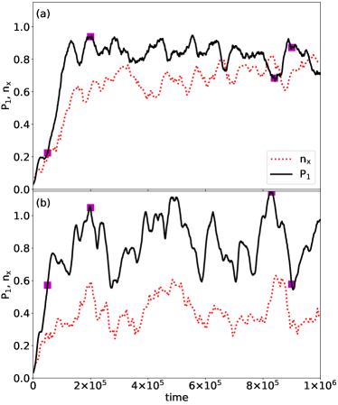
Figure 1: Structural order measurements $n_{x}$ (red), the fraction of disks located in the bulk of crystalline clusters, and $P_{1}$ (black), a machine-learning derived order parameter, vs time in simulation time steps for samples with $\phi=0.47$. The persistence time is (a) $\tau=1\times 10^{5}$ and (b) $\tau=1\times 10^{6}$. Purple squares indicate the times at which the disk images in Fig. 2 were obtained.

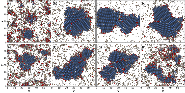
Figure 2: Time evolution of two simulations of actively propelling disks at a density of $\phi=0.47$ for (a-d) $\tau=1\times 10^{5}$ and (e-h) $\tau=1\times 10^{6}$. The systems are shown at times of (a) $5\times 10^{4}$, (b) $2\times 10^{5}$, (c) $8.3\times 10^{5}$, (d) $9\times 10^{5}$, (e) $5\times 10^{4}$, (f) $2\times 10^{5}$, (g) $8.4\times 10^{5}$, and (h) $9\times 10^{5}$. These times are marked with purple squares in Fig 1. The disks are colored according to whether they belong to the crystalline fraction $n_{x}$ (blue), the gaseous fraction $n_{g}$ (tan), or the cluster edges $n_{e}$ (red) as determined by the bond orientational order parameter measurement.

In Fig. 1(a) we plot the structural order measures $n_{x}$ and $P_{1}$ as a function of time for a system with $\phi=0.47$ at a persistence time of $\tau=1\times 10^{5}$, and in Fig. 1(b) we show the corresponding measures for a sample with the same density and $\tau=1\times 10^{6}$. Since the simulations are initialized with the disks in random, non-overlapping positions, there is no initial structural order, and both $n_{x}$ and $P_{1}$ are low at early times. The system quickly assembles into a MIPS state, with a single large cluster forming within about $t=1\times 10^{5}$ simulation time steps. For the sample with $\tau=1\times 10^{5}$, both $P_{1}$ and and $n_{x}$ grow rapidly at early times and reach a steady state with $n_{x}\sim 0.7$ for $t>1\times 10^{5}$. These quantities then fluctuate by approximately 10% throughout the remainder of the simulation. When $\tau=1\times 10^{6}$, the overall behavior is similar but the fluctuations in the steady state are more pronounced. Additionally, the steady state value of $n_{x}$ for $\tau=1\times 10^{6}$ is only $n_{x}\sim 0.41$, indicating that the clusters are less stable for the larger value of $\tau$. In both samples we find that peaks and valleys in $P_{1}$ and $n_{x}$ are correlated with each other, and this behavior is most clearly visible in the sample with $\tau=1\times 10^{6}$.

In Fig. 2 we illustrate the positions of the disks in a time sequence extracted from the time series of Fig. 1 in order to determine whether the peaks and valleys occurring in $P_{1}$ and $n_{x}$ in Fig. 1 are correlated with structural changes in the system. Figure 2(a-d) shows images from the sample with $\tau=1\times 10^{5}$ and Fig. 2(e-h) is for the sample with $\tau=1\times 10^{6}$. The disks are colored according to whether they belong to the crystalline $n_{x}$ subset, the gaseous $n_{g}$ subset, or the edge $n_{e}$ subset according to the bond orientational order parameter measurement. At early times, as shown for $t=5\times 10^{4}$ in Fig. 2(a,e), only small clusters have evolved from the initial disordered state of the system, indicating that smaller clusters are associated with small values of $P_{1}$ and $n_{x}$. The ML algorithm is able to discern the average cluster size, with $P_{1}$ = 0.25 for $\tau=1\times 10^{5}$ where the incipient crystalites are small, but $P_{1}$ = 0.55 for $\tau=1\times 10^{6}$ where the incipient crystalites are larger. While both $P_{1}$ and $n_{x}$ make use of interparticle distances and local structural information, $P_{1}$ in general performs better than $n_{x}$ in detecting crystalline signatures since it is able to capture ordering that extends beyond the nearest neighbors.

Figure 2(b,f) shows that for both values of $\tau$, a large active cluster forms at $t=2\times 10^{5}$. Here $P_{1}\approx 1.0$. At longer times in the $\tau=1\times 10^{5}$ sample, both $P_{1}$ and n_x remain large with $P_{1}\approx 0.9$ and $n_{x}\approx 0.7$, indicating that the cluster size reaches a steady state. This is consistent with the stable large cluster visible in Figs. 2(c) and (d). The morphology of the cluster continues to evolve as a function of time, with grain boundaries forming and then disappearing, but the overall size of the cluster remains nearly constant once it has formed. In contrast, although a large cluster is still present in the $\tau=1\times 10^{6}$ system at $t=8.4\times 10^{5}$, as shown in Fig. 2(g), this is followed by the rapid disassembly event illustrated in Fig. 2(h). When the cluster disassembles, $P_{1}$ drops to $P_{1}\approx 0.6$ and $n_{x}$ also shows a less pronounced drop. In the supplementary information we include a video illustrating the disassembly of the cluster for this time interval supplementary information. . As indicated by the recovery of the value of $P_{1}$ at later times in Fig. 1(b), the cluster repeatedly reforms and disassembles for this value of $\tau$. Thus, although there is clustering for both $\tau=1\times 10^{5}$ and $\tau=1\times 10^{6}$, the $\tau=1\times 10^{5}$ cluster is stable while the $\tau=1\times 10^{6}$ cluster is strongly fluctuating.

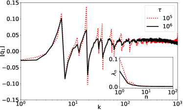
Figure 3: $[q_{1}]$, the first row of the total transformation matrix $\vec{Q}=\vec{W}\vec{W}_{0}$, vs component number $k$ for the system in Figs. 1 and 2 with $\phi=0.47$ at $\tau=1\times 10^{5}$ (red) and $\tau=1\times 10^{6}$ (black). This measure illustrates how PCA effectively weights $g(r)$. Inset: The normalized PCA eigenvalues $\lambda_{n}$ vs $n$ for the same samples.

Both $P_{1}$ and $q_{6m}$ are affected by the number of particles participating in the largest active cluster and the local ordering of particles. In general, $P_{1}$ captures more information than $q_{6m}$. To demonstrate this, in Fig. 3 we plot the metrics derived from PCA for the entire time series obtained for the systems in Fig. 1 and Fig. 2 with $\tau=1\times 10^{5}$ and $\tau=1\times 10^{6}$. The main panel of Fig. 3 is a plot of the components of $[q_{1}]$, the first row of the total transformation matrix $\vec{Q}=\vec{W}\vec{W}_{0}$, versus component number $k$. Since the $\vec{Q}$ metric contains a geometric snapshot of the neighbor environment for many probe particles, the quantity $[q_{1}]$ provides information similar to the radial distribution function $g(r)$, with increasing $k$ corresponding to increasing values of $r$ due to the fact that the feature vectors $\vec{f}$ have been sorted according to size. The PCA effectively performs a weighting of $g(r)$, as described in more detail in Ref. McDermott et al. (2020), and in Fig. 3 we observe that the weightings differ when $\tau$ is varied. At $\tau=1\times 10^{5}$, where stable large clusters form, $[q_{1}]$ is strongly peaked at the regular spacings expected for a crystalline lattice out to relatively large distances, indicating that PCA has detected longer range crystalline ordering. In contrast, for $\tau=1\times 10^{6}$, the weight at these crystalline peaks is diminished and is replaced by greater weight at a continuum of longer distances, representative of the increased amount of gas phase present. The inset of Fig. 3 shows the normalized eigenvalues $\lambda_{n}$ sorted by magnitude, corresponding to the ranked principal components plotted as a function of element index $n$. This is a typical performance measurement of PCA’s ability to reduce the dimensionality of the feature space. Here the rapid decrease in $\lambda_{n}$ with $n$ demonstrates that the first few principal components are able to capture most of the information in the data set. The ratio of $\lambda_{1}$ to $\lambda_{2}$ is higher for $\tau=1\times 10^{5}$ than for $1\times 10^{6}$, indicating that more of the feature space can be described by the first principal component in the $\tau=1\times 10^{5}$ system. This is consistent with the enhanced amount of crystalline ordering that appears at $\tau=1\times 10^{5}$.

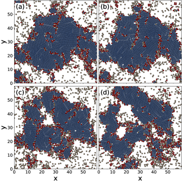
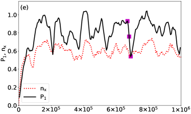
Figure 4: (a-d) Illustration of the time evolution of the formation of a void in a sample with $\phi=0.6$ and $\tau=1\times 10^{5}$. The system is shown at times of (a) $6.7\times 10^{5}$, (b) $6.72\times 10^{5}$, (c) $6.8\times 10^{5}$, and (d) $7.0\times 10^{5}$. The disks are colored according to whether they belong to $n_{x}$ (blue), $n_{g}$ (tan), or $n_{e}$ (red). An animation of this time sequence is available in the supplemental material supplementary information. . (e) Time series of $P_{1}$ (black) and n_x (red) for the same system. Times $6.7\times 10^{5}$, $6.8\times 10^{5}$, and $7.0\times 10^{5}$, corresponding to the interval illustrated in panels (a-d), are highlighted with purple squares. We note that the times of panels (a) and (b) are so close together that they overlap on the scale of the squares, so only the time of panel (a) is shown.

To show more clearly how time-resolved $P_{1}$ values correlate with the actual dynamics of the system, in Fig. 4(a-d) we illustrate the particle positions during the destruction of a large cluster due to a void formation process for a system with $\phi=0.6$ and $\tau=1\times 10^{6}$. The fragments of grain boundaries visible as chains of red particles in Fig. 4(a) coalesce into a prominent longer and thicker grain boundary in Fig. 4(b). The evolution of the grain boundaries is controlled in part by the one-dimensional string-like motion of vacancies through the crystalline regions Pertsinidis and Ling (2001); Dudarev (2003); Smallenburg et al. (2012); Lechner et al. (2013), visible as white streaks in the figure. A vacancy cannot remain stable inside the crystalline region but travels quite rapidly toward vacancy sink areas Swanson (1982) consisting of grain boundaries and the edges of the cluster. The vacancies can move at speeds considerably higher than the motion of a free individual disk, and their movement also becomes increasingly one-dimensional as the density of the system becomes higher van der Meer et al. (2018). In Fig. 4(c), continued absorption of vacancies by the grain boundary results in the opening of a void area that serves as a vacancy sink location, and the effectiveness of this sink increases as the outer contour of the void becomes longer. Further growth of the void causes the cluster to break apart, as illustrated in Fig. 4(d). We find that when $\tau=1\times 10^{5}$, vacancies are short lived and tend to be reabsorbed by the crystal almost as quickly as they form, while when $\tau=1\times 10^{6}$, the vacancies are able to persist for much longer times and can travel distances on the order of the size of the cluster. This can also be seen in the supplemental movies supplementary information. .

In Fig. 4(e), we plot $n_{x}$ and $P_{1}$ versus time for the $\phi=0.6$ and $\tau=1\times 10^{6}$ system illustrated in Fig. 4(a-d). The purple squares correspond to the times at which images of the void formation and growth were obtained. Although there is a weak dip in $n_{x}$ over this time interval, it is difficult to tell from $n_{x}$ that anything unusual is happening to the cluster structure. In contrast, $P_{1}$ exhibits a pronounced dip as the cluster disintegrates. When the cluster is still largely intact in Fig. 4(a,b), $P_{1}$ has a high value of $P_{1}\approx 0.9$, but when the cluster splits apart, $P_{1}$ drops to $P_{1}\approx 0.59$. The reassembly of the cluster (not illustrated) at slightly later times is accompanied by a recovery of the value of $P_{1}$ back to its former level of $P_{1}\approx 0.9$. This shows that $P_{1}$ captures many more features than are found in standard measures used to characterize MIPS, and that even the time evolution of $P_{1}$ contains useful information.

V Velocity Fluctuations and Noise Power

Since we have obtained a time-dependent measure capable of capturing the evolution of the MIPS structure in the steady state, it is interesting to examine the time series of related fluctuating quantities in more detail. For many systems such as magnetic domain walls Sethna et al. (2001); Durin and Zapperi (2005), charge density waves, Grüner (1988), Wigner crystals Reichhardt and Olson Reichhardt (2004), and vortices in type-II superconductors Marley et al. (1995); Field et al. (1995); Olson et al. (1998); Okuma et al. (2008); Reichhardt and Reichhardt (2017), under application of an external drive it is possible to analyze fluctuations in the velocity or resistance for different conditions. In the active matter system, the net velocity is zero since there is no net bias in the run-and-tumble motion and on average the particles move in all directions at once; however, we can still measure the average speed of all the particles as a function of time since this quantity remains finite. We compute the average speed $\langle V\rangle$ according to:

$$\langle V\rangle=\frac{1}{N_{d}}\sum_{i}^{N_{p}}\sqrt{(\vec{v}_{i}\cdot{\hat{x}})^{2}+(\vec{v}_{i}\cdot{\hat{y}})^{2}}$$ (6)

where the average is taken over all particles at an instant in time.

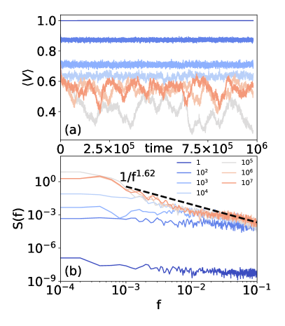
Figure 5: (a) Average speed $\langle V\rangle$ vs time for samples with $\phi=0.45$ and $\tau=1$, 100, $10^{3}$, $10^{4}$, $10^{5}$, $10^{6}$, and $10^{7}$, from top to bottom. The curves are colored according to the legend in panel (b). (b) Noise spectra $S(f)$ obtained from the time series in panel (a). The dashed line indicates a fit to $S(f)\propto 1/f^{\alpha}$ with $\alpha=1.62$.

In Fig. 5(a) we plot $\langle V\rangle$ vs time for systems with $\phi=0.45$ at $\tau=1\times 10^{0}$, $1\times 10^{2}$, $1\times 10^{3}$, $1\times 10^{4}$, $1\times 10^{5}$, $1\times 10^{6}$, and $1\times 10^{7}$. For $1<\tau<1\times 10^{4}$, the system is in a fluid phase where $\langle V\rangle$ fluctuates weakly and the magnitude of $\langle V\rangle$ decreases monotonically with increasing $\tau$. When $\tau=1$, every particle tumbles at every timestep so the persistence of the motion drops to zero and the particle motion is unimpeded, giving $\langle V\rangle=F^{a}=1$. As $\tau$ increases in the fluid state, more collisions occur between particles, causing them to slow and decreasing the average speed. Some small clusters begin to form for $\tau=1\times 10^{4}$, leading to an increase in the characteristic time scale of fluctuations in $\langle V\rangle$. At $\tau=1\times 10^{5}$ the system has entered the MIPS phase, where there are large fluctuations in $\langle V\rangle$ and we observe formation of a large cluster. For $\tau=1\times 10^{6}$ and $1\times 10^{7}$, the system is still in a MIPS state but the fluctuations of $\langle V\rangle$ are diminished and the magnitude of $\langle V\rangle$ has increased compared to the $\tau=1\times 10^{5}$ system, consistent with the clusters being more stable at $\tau=1\times 10^{5}$ than at $\tau=1\times 10^{6}$, as described in Section IV.

The time series of $\langle V\rangle$ can be characterized with the power spectrum

$$S(f)=\left|\int\langle V(t)\rangle\exp{(i2\pi ft)}dt\right|^{2}\ ,$$ (7)

where $f=2\pi\omega$ is the frequency. Note that this measure differs from the density fluctuations examined in previous work Fily and Marchetti (2012). In Fig. 5(b) we plot $S(f)$ for the time series from Fig. 5(a). For $\tau=1$, $S(f)$ is nearly flat across six decades of frequency, indicative of white noise. As $\tau$ increases, we find a transition from white noise to a power law spectrum with

$$S(f)\propto f^{-\alpha}\ ,$$ (8)

where the amount of noise power at low frequencies increases significantly in the power law regime. For $\tau=1\times 10^{5}$ we obtain a fit to $\alpha=1.62$ using the algorithm in Ref. Alstott et al. (2014). We find similar values of $\alpha$ for $\tau=1\times 10^{6}$ and $1\times 10^{7}$, although both the range of the power law and the magnitude of the low frequency noise power are greatest at $\tau=1\times 10^{5}$.

Transitions from white noise to $1/f^{\alpha}$ noise accompanied by peaks in the low frequency noise power are observed in many driven systems that exhibit depinning Reichhardt and Reichhardt (2017). In experiments on the depinning of superconducting vortices, Marley et al. Marley et al. (1995) found exponents ranging from $\alpha=1.5$ to $\alpha=2.0$ in the peak effect region, where the motion of the vortices is expected to be plastic. In studies of vortex avalanches, exponents of $\alpha=1.5$ were observed in the power law distribution of avalanche sizes for drives just above depinning, while $\alpha$ increased to $\alpha=2.0$ as the driving rate was increased Field et al. (1995). In simulations of the depinning of 2D vortex assemblies, $\alpha\approx 1.5$ to $1.9$ depending on the strength of the quenched disorder in the sample Olson et al. (1997, 1998); Reichhardt and Reichhardt (2017). Simulations of yielding transitions in 2D amorphous solids undergoing avalanches have produced power law dependences with $\alpha=1.25-1.35$ Regev and Lookman (2019).

Power law behavior arises near a critical point because the diverging length scales that emerge lead to larger and larger amounts of low frequency noise. For the nonequilibrium random field Ising model near a disorder-induced nonequilibrium critical point, noise power spectra with $\alpha=1.77$ are observed Travesset et al. (2002), and the relationship between the value of $\alpha$ and the critical exponents associated with the transition is given by $\alpha=1/\sigma\nu z$. Chen and Yu Chen and Yu (2007) examined noise fluctuations in Ising and Potts models and found that the noise power of energy fluctuations reaches a maximum at the magnetic phase transition, with white noise appearing above and below the transition. For the Ising model, $\alpha=1.0$, while for the Potts model, $\alpha=1.56$. If magnetization fluctuations are considered instead of energy fluctuations, power law noise still arises with $\alpha=1.8$ for the Ising model and $\alpha=1.7$ for the Potts model.

VI $\phi-\tau$ Heat Diagrams

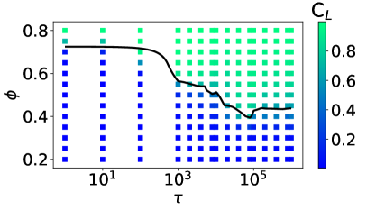
Figure 6: (b) Heat map of $C_{L}$, the fraction of particles in the largest cluster, as a function of $\phi$ vs $\tau$. The black line indicates points where $C_{L}=0.5$.

One of the most common measures of motility-induced phase separation is the fraction of particles $C_{L}$ contained in the largest connected cluster. This measure is similar to $n_{x}$ but does not distinguish whether the arrangement of the particles is crystalline; it only determines whether the particles are in contact with each other. In Fig. 6, we plot a heat map of $C_{L}$ as a function of $\phi$ vs $\tau$; the black line indicates points where $C_{L}=0.5$. We observe MIPS phases for $\tau\geq 1\times 10^{3}$. For $\tau<1\times 10^{3}$ and $\phi>0.7$, the system is sufficiently dense that the value of $C_{L}$ is large, but this is the result of a percolating network of particle-particle contacts rather than the formation of a MIPS cluster. For $0.4<\phi<0.5$ and $1\times 10^{4}<\tau<1\times 10^{6}$, $C_{L}$ exhibits reentrance as a function of $\tau$. Since $C_{L}$ can only distinguish between the presence or absence of extended networks of particle contacts, and cannot distinguish a cluster from a percolating contact network, it is necessary to turn to other measures to determine whether additional subphases exist within the MIPS state, such as the stable and unstable clusters described in Section IV for different values of $\tau$.

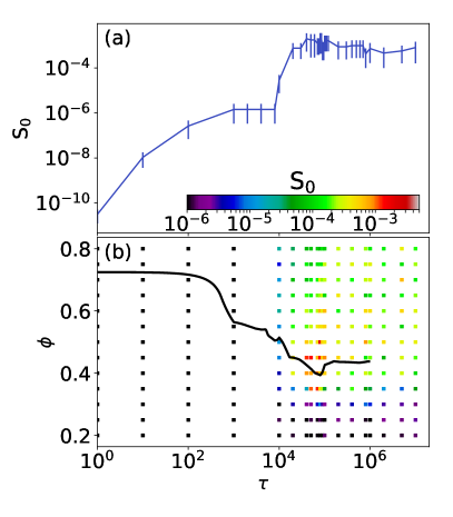
Figure 7: (a) Low frequency noise power $S_{0}$ versus $\tau$ for samples with $\phi=0.45$. (b) Heat map of $S_{0}$ as a function of $\phi$ vs $\tau$. Black points indicate denote $(\phi,\tau)$ pairs for which the noise is white and $S_{0}$ has a very low value.

In Fig. 7(a) we plot the noise power $S_{0}$ versus $\tau$ for a sample with $\phi=0.45$. To obtain the noise power, we integrate $S(f)$ over a small interval at low frequencies,

$$S_{0}=\int_{f_{0}}^{f_{1}}S(f)df\ .$$ (9)

We average the measurement of $S_{0}$ over several intervals $(f_{0},f_{1})$ and report the measure with an associated error. We find that $S_{0}$ increases steadily from $\tau=1$, with a sharp increase occurring near $\tau=1\times 10^{4}$. The noise power reaches a peak near $\tau=5\times 10^{4}$, and stabilizes onto a plateau for $\tau>1\times 10^{5}$.

Figure 7(b) shows a heat map of $S_{0}$ plotted as a function of $\phi$ versus $\tau$. In the fluid phase, the noise power is low and the power spectra are white. For $\phi>0.75$ and $\tau<1\times 10^{3}$, the noise is low and the power spectra are white even though $C_{L}$ is high, indicating that the system is not in the MIPS state. We find that $S_{0}$ is nonmonotonic and reaches its highest values for $5\times 10^{4}\leq\tau\leq 5\times 10^{5}$ and $0.35<\phi<0.55$, which is also the region where $C_{L}$ becomes reentrant as a function of $\tau$. In this regime, the velocity noise has a $1/f^{\alpha}$ signature with $\alpha\approx 1.6$. Elsewhere in the MIPS regime, the velocity noise still has a $1/f^{\alpha}$ tail but the value of $S(f)$ saturates at low frequencies, whereas in the critical regime where $S_{0}$ is largest, the power law behavior of the velocity noise extends over the greatest range of frequencies. The black line indicates the points at which $C_{L}=0.5$, showing that more information can be extracted from the behavior of $S_{0}$ than from the behavior of $C_{L}$ alone. In particular, the noise measurement captures some features outside of the boundary delineated by the $C_{L}$ measurement. Near $\tau=1\times 10^{5}$ there is large noise all the way down to $\phi=0.3$, while the cluster measurement was only large down to $\phi=0.4$. At the low density of $\phi=0.3$, there are short-lived loosely packed clusters in which the particle speed drops, but these clusters are not compact enough to register in the $C_{L}$ measurement.

The results in Fig. 7(a) are similar to the noise power measurements obtained in driven systems, where a maximum in the noise power occurs at a dynamical transition and is then followed by a decrease in noise. Chen and Yu found that the noise power peaks at the critical point for equilibrium phase transitions Chen and Yu (2007). For driven systems with quenched disorder that undergo plastic depinning, such as superconducting vortices, there is a peak in the noise power within the plastic flow phase where strong distortions of the vortex lattice are occurring. The noise power decreases when the system is more strongly driven since the number of plastic events is reduced Marley et al. (1995); Olson et al. (1998); Reichhardt and Reichhardt (2017). In the active system, as $\tau$ increases, the cluster structure becomes more crystalline and fewer plastic events occur. For $\phi>0.55$, the peak in $S_{0}$ is reduced in magnitude and becomes more of a plateau. This suggests that the transition into the MIPS state has properties associated with a critical phase transition, and that in the region spanning $0.35<\phi<0.6$ these critical properties are visible, while for larger $\phi$ and higher $\tau$, the system is not critical.

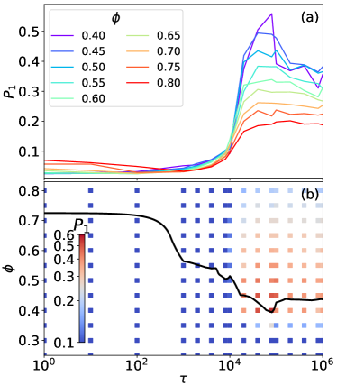
Figure 8: (a) P₁ vs $\tau$ for varied disk density $\phi=0.4$ (purple), 0.45, 0.5, 0.55, 0.6, 0.65, 0.7, 0.75, and 0.8 (red), from top to bottom. (b) Heat map of $P_{1}$ as a function of $\phi$ vs $\tau$. The black line indicates points at which $C_{L}=$ 0.5. This figure was composed using 500 GB of feature data extracted from 90 simulations.

We next measure $P_{1}$ for varied $\tau$ and $\phi$ to see whether the ML detects features that are similar or different from what appears in $C_{L}$ and $S_{0}$. In Fig. 8(a) we plot P₁ versus $\tau$ for samples with $\phi=0.4$, 0.45, 0.5, 0.55, 0.6, 0.65, 0.7, 0.75, and 0.8. Here, feature data are evaluated every $1\times 10^{5}$ timesteps across 10⁶ simulation steps and combined into a single matrix for evaluation of principal components. For $\tau>10^{6}$, it becomes difficult to analyze the data. In the liquid phase, $P_{1}$ is low even for $\phi=0.8$ where $C_{L}$ is high. For $0.4<\phi<0.55$ in the lower density portion of the MIPS regime, there is a peak in $P_{1}$ that also coincides with the peak in $S_{0}$. For $\phi>0.55$, $P_{1}$ decreases and saturates to a level higher than its value in the liquid phase, since MIPS is still present. In Fig. 8(b), we plot a heat map of $P_{1}$ as a function of $\phi$ versus $\tau$ along with the boundary line indicating the points where $C_{L}=0.5$. The structure of $P_{1}$ is similar to that of $S_{0}$, with the largest values of $P_{1}$ occurring in the low density, intermediate $\tau$ portion of the MIPS regime.

VII Discussion

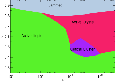
Figure 9: A schematic of the possible regimes inside the MIPS state as a function of $\phi$ vs $\tau$ showing a jammed crystal, an active crystal, a critical region, and an active liquid.

The different features in $C_{L}$, $S_{0}$, and $P_{1}$ suggest that there could be different regimes within the MIPS phase. For example, at high $\phi$ and high $\tau$, $P_{1}$ and $S_{0}$ have intermediate values but $C_{L}$ is high. This regime could be described as consisting of active crystals where there are still fluctuations or intermittent motion giving rise to avalanche-like rearrangements inside the crystals, but the size of these rearrangements is cut off so that the magnitude of the low-frequency noise is reduced. Mandal et al. Mandal et al. (2020) considered the limit of dense active systems and varied both the motor force and the persistence time. At small motor forces, the system is in a dynamically arrested state but is still active so that it can be described as an active crystal. At high motor forces the system shows intermittent plastic yielding, while for even higher motor forces, the system becomes a liquid due to interpenetration of the particles. A similar breakdown of clustering due to particle interpenetration was observed earlier Fily et al. (2014). In our case, we hold the motor force fixed so that particle interpenetration remains unimportant even as the density increases. For high density and larger values of $\tau$, our system remains in the active crystal state but becomes more frozen and exhibits reduced intermittency. We argue that for the dense system, the noise will be small in the active crystal but high when the motor force becomes large enough to induce plastic deformations. Such deformations would give rise to a $1/f^{\alpha}$ velocity fluctuation signature and large noise, and the noise power would decrease again in the active liquid state. For dense systems with very low persistence length, the system behaves more like a jammed solid with low noise and low $P_{1}$. The critical regime we find where $P_{1}$ and $S_{0}$ are large could be associated with a second-order transition into the MIPS phase or some other type of critical regime similar to the criticality associated with plastic depinning. The critical regime is characterized by high $C_{L}$, high $P_{1}$, and high $S_{0}$. In Fig. 9, we plot a suggested schematic phase diagram as a function of $\phi$ versus $\tau$ showing an active liquid, a jammed phase, an active crystal, and a critical phase.

Our results suggest that the dynamics of vacancies play an important role in determining whether the large MIPS cluster can remain stable once it forms in the critical cluster regime, or whether the cluster will repeatedly break apart and reform in the active crystal regime. If we focus on the nucleation of a single vacancy, a nucleation attempt can succeed if a neighboring particle does not move into the newly formed vacancy location Zhurkov (1965). The neighboring particle is confined by the nearly crystalline surrounding cage of dense phase, and explores different directions of this cage at a rate of $1/\tau$. When $\tau$ is low enough, the neighboring particle changes running directions frequently and can explore the entire cage rapidly. The rate of vacancy discovery decreases with increasing $\tau$, so that for high $\tau$ the ability to fill the vacancy decreases with increasing $\tau$ since the neighboring particle is unable to find the vacancy efficiently. As a result, vacancies are filled at a maximal rate for the low $\tau$ and low $\phi$ portion of the MIPS state, resulting in the emergence of a critical cluster regime.

At low $\phi$ there is no MIPS state because the collision frequency between particles drops to values that are too low to sustain clusters. The clusters are the most stable at the onset of MIPS and become less stable as $\phi$ increases. Vacancies can nucleate anywhere inside an active solid and are not limited to surface sites or favorable locations such as grain boundaries. Given a crystalline patch of dense phase, there is some rate $R$ per unit surface area at which vacancies can nucleate per unit time. As a result, the total number $N_{v}$ of vacancies that nucleate in a given time period is proportional to the total surface area $A$ of the cluster. The fraction $C_{L}$ of particles in the largest cluster remains nearly constant as a function of $\phi$ within the MIPS state, and the dense phase is a close-packed crystal of particles so its density does not vary with $\phi$. Thus $A$ must increase with increasing $\phi$ when $C_{L}$ remains constant since there are more particles in the system. The total number of vacancy nucleation attempts therefore increases with increasing $\phi$. The nucleation success rate is determined by the value of $\tau$ as described above. The largest stable clusters appear when a low number of nucleation attempts is combined with a low nucleation success rate, and this situation occurs for intermediate $\tau$ at densities that are just above the transition into the MIPS state. For higher values of $\tau$ or $\phi$, a larger number of vacancies successfully nucleate inside the active crystal, where they can cluster into voids and destabilize the crystal as a function of time, resulting in the emergence of the active crystal state.

VIII Summary

We have analyzed motility-induced phase separation in a two-dimensional active disk system using noise analysis and a machine learning principal component analysis (PCA). We show that PCA can capture time-dependent features such as cluster rearrangements and breakups better than standard structural measures such as the fraction of particles in the largest cluster. We also compute the power spectra of the time fluctuations in the average speed of the particles and find that in the active fluid, the noise is white and the noise power is low, but in the MIPS state, the noise has a $1/f^{\alpha}$ signature with $\alpha=1.6$, similar to what is found in depinning systems or systems in a critical state. We find that the PCA principal component and the noise power can be combined along with cluster size to characterize different dynamic states within MIPS. For intermediate persistence lengths and densities, we find that the principal component and noise power are large and there is a reentrant feature in the cluster size. At large densities and high persistence length the principal component is low and the noise power is immediate, while in the active fluid phase, all of the quantities are low. From these measures, we propose that the MIPS state can be divided into an active crystal phase, a critical MIPS phase, and a jammed phase, in addition to the fluid phase that occurs outside of the MIPS regime.