subsection subsubsection

Compositional nonlinear audio signal processing with Volterra series

Abstract

We develop a compositional theory of nonlinear audio signal processing based on a categorification of the Volterra series. We begin by considering what it would mean for the Volterra series to be functorial with respect to a base category whose objects are temperate distributions and whose morphisms are certain linear transformations. This leads us to derive formulae describing how the outcomes of nonlinear transformations are affected if their input signals are first linearly processed – e.g., translated, modulated, sampled, or periodized. We then consider how nonlinear audio systems, themselves, change, and we introduce as a model thereof a notion of morphism of Volterra series, which we exhibit as a type of lens map. We show how morphisms can be parameterized and used to generate indexed families (e.g., sequences) of Volterra series, which are well-suited to model nonstationary or time-varying nonlinear phenomena. We then describe how Volterra series and their morphisms organize into a category, which we call Volt. We exhibit the operations of sum, product, and series composition of Volterra series as monoidal products–which are bifunctors on Volt–and we identify, for each in turn, its corresponding universal property. In particular, we show that the series composition of Volterra series is associative. We then bridge between our framework and a subject that is at the heart of audio signal processing: time-frequency analysis. Specifically, we show that a known equivalence, between a class of second-order Volterra series and the bilinear time-frequency distributions (TFDs), can be extended to one between certain higher-order Volterra series and the so-called polynomial TFDs. We end by outlining potential avenues for future work, including the incorporation of nonlinear system identification techniques and the potential extension of our theory to the settings of compositional graph and topological audio signal processing.

Contents

1. Introduction
2. 1 The Volterra series
   1. 1.1 Volterra series basics
      1. 1.1.1 Frequency domain representation
      2. 1.1.2 Kernel symmetry
      3. 1.1.3 Parametricity
   2. 1.2 Multilinear maps and the tensor product
      1. 1.2.1 Tensor algebra, $T(S_{\mathbb{R}})$
   3. 1.3 Multivariate Volterra series
   4. 1.4 Volterra series representations of some simple systems
3. 2 The Volterra series as a functor
   1. 2.1 Categories and functors
   2. 2.2 The category $S^{\prime}(\mathbb{R})$
   3. 2.3 The Volterra series as a functor
   4. 2.4 Examples of the action of a VS on a linear transformation
      1. 2.4.1 Translation (time shift)
      2. 2.4.2 Modulation (frequency shift)
      3. 2.4.3 Periodization
      4. 2.4.4 Sampling
4. 3 The category of Volterra series
   1. 3.1 Natural transformations
   2. 3.2 Morphisms of Volterra series
      1. 3.2.1 Morphisms as lens maps
      2. 3.2.2 Parameterized morphisms
      3. 3.2.3 Naturality of Volterra morphisms
   3. 3.3 Volterra series form a category
5. 4 Volt as a monoidal category
   1. 4.1 Monoidal categories
   2. 4.2 Sum and product of Volterra series
   3. 4.3 Series Composition
      1. 4.3.1 Associativity of $\triangleleft$
6. 5 Time-frequency signal processing using Volterra series
   1. 5.1 Time and frequency
      1. 5.1.1 Bilinear time-frequency distributions
         1. 5.1.1.1 The role and properties of the Wigner-Ville Distribution
      2. 5.1.2 Volterra series representation of Cohen’s class
   2. 5.2 Higher-order and polynomial time-frequency distributions
      1. 5.2.1 The Polynomial Wigner-Ville Distribution
      2. 5.2.2 Volterra series representation of the Polynomial WVD
7. Conclusion and prospects
8. Appendix A: Construction of the category $S^{\prime}(\mathbb{R})$
9. Appendix B: Proof of the associativity of $\vartriangleleft$

Notation

$\omega=2\pi f$—angular frequency
$\boldsymbol{\omega}\in\mathbb{R}^{n}$—an $n-$dimensional vector
$f:X\rightarrow Y$—a map from a space $X$ to a space $Y$
$D^{C}$—the space of mappings from $C$ to $D$
$S(\mathbb{R})$—the semicategory of signals
$S^{{}^{\prime}}(\mathbb{R})$—the category of temperate distributions
$F:S^{{}^{\prime}}(\mathbb{R})\rightarrow S^{{}^{\prime}}(\mathbb{R})$—the Fourier transform
$s\in S(\mathbb{R}^{n})$—an $n-$signal
$\hat{s}=F(s)\in S^{{}^{\prime}}(\mathbb{R}^{n})$—an $n-$spectrum
$T^{k}(W)$—the $k^{\text{th}}-$tensor power of a vector space $W$
$T(W)=\bigoplus_{k=0}^{\infty}T^{k}(W)$—the tensor algebra of $W$
$s^{\otimes j}$—the $j-$fold iterated tensor product of $s$ with itself
$(B\triangleleft A)(-)=B(A(-))$—the series composition of $A$ and $B$

Introduction

A nonlinear system $V$ is one whose response to a set of inputs may be more than the sum of its responses to each of the inputs independently; that is, its behavior may fail to satisfy the properties of superposition

$$V[s+s^{{}^{\prime}}]\neq V[s]+V[s^{{}^{\prime}}]$$ (1)

and scaling

$$V[\alpha s]\neq\alpha V[s]$$

for all signals $s,s^{\prime}$ and scalar $\alpha$.

But nonlinearity is only a negativistic notion. The departure of a nonlinear system from linearity could, instead, be written positively, in terms of one or more nonlinear effects: for example

$$V[s+s^{{}^{\prime}}]=V[s]+V[s^{{}^{\prime}}]+\gamma(s,s^{\prime}),$$ (2)

where $\gamma$ is a function that now encodes the nonlinear part and depends on both the inputs $s$ and $s^{{}^{\prime}}$. But how do nonlinear effects arise, and how can the function $\gamma$ be described?

The Volterra series (VS) is a universal and combinatorially complete model of nonlinear dynamics that provides a concrete answer to these questions. Roughly, it says that nonlinear effects arise as sums of weighted interactions between the samples of (various combinations of) the input signals. More precisely, a Volterra series consists of a collection of weights that measure the strength of a nonlinear system’s response to each possible multiplicative interaction of the samples amongst each possible combination of input signals, taken with repetition (allowing self-interactions) and counting permutations.

As the focus of this work is on the nonlinear processing of conventional audio, and on the structure of nonlinear audio systems and their transformations, it deals near-to-exclusively with nonlinear systems that process one or many streams of audio data. However, the abstract form of the Volterra series is more generally capable of describing nonlinear systems that process inputs from other types of domains, such as signals over graphs or topological spaces. Thus, the relevance is to the broader context of nonlinear systems theory and topological signal processing.

The domain of audio moreover provides a fruitful testbed for the development of a general theory of nonlinear signal processing, since nonlinear effects in audio abound, and their representations in the frequency domain are relatively well understood both mathematically and intuitively. For example, intermodulation, harmonic and inharmonic distortion, and nonlinear resonance are all classes of nonlinear phenomena that are routinely experienced acoustically by audio engineers and musicians. The frequency domain form of the VS affords, in this light, a mathematical syntax that maps well onto an audio-based semantics.

Overview

In Chapter 1, we motivate the VS and briefly survey the core variants that have been introduced in the literature, observing the various facets of the same mathematical object that are illuminated by the different definitions. We begin by reviewing the univariate Volterra series in both its time and frequency domain forms. We then prepare the lift to the multivariate case by rewriting the univariate series using the tensor product, and recall the universal property of the tensor product, as well as the tensor power and tensor algebra constructions. We then review the multivariate VS and show how, in a certain precise sense, it is combinatorially complete. We then briefly review the VS with parametrized kernels.

In Chapter 2, we address the question of how the result of processing an input signal by a nonlinear system changes if the signal is first transformed linearly. For example, what happens if the input is translated or modulated before processing; can we derive an associated linear transformation from the nonlinear one? To answer this question, we ask what it would mean if the Volterra series, instead of being defined an operator acting only on signals, were instead characterized as an endofunctor on the category, denoted $S^{{}^{\prime}}(\mathbb{R})$, of tempered distributions signals and multiplier-type operators which is introduced in Appendix A. We then catalogue the Volterra series representations of certain elementary linear and nonlinear operators.

In Chapter 3, we introduce a mechanism for how nonlinear systems modeled by Volterra series change; that is, we define a notion of morphism of Volterra series, which we define as a lens map and conjecture is a natural transformation between them. Volterra series morphisms enable us to speak about the networks of ways that different nonlinear systems are functionally related to one another, and allow us to define a category of Volterra series, which we call Volt.

In Chapter 4, we study three basic ways — sum, (categorical) product, and series composition — of combining Volterra series. For each, we write down the universal morphism induced by the combination, and in Appendix B we prove the associativity of the most complex of the three: the series composition product, $\triangleleft$. In so doing, we effectively exhibit Volt as a symmetric monoidal category, with series composition as the monoidal (tensor) product. This in principle enables nonlinear systems and their interconnections to be modeled in a rigorous diagrammatic way by Volterra series, in a manner analogous to how circuit diagrams or signal flow graphs are used to model interconnections of linear systems.

Having built up the theoretical framework and categorical structure of Volterra series in Chapters 2, 3, and 4, in Chapter 5 we apply our newly developed theory to a subject at the heart of audio signal processing: time-frequency distributions (TFDs). We first recapitulate a result of Powers and Nam [2], in which they showed that the time-frequency shift-covariant TFDs of Cohen’s class are equivalent to certain class of double, second-order Volterra series. We then extend the equivalence to the realm of time-multifrequency, or higher-order time-frequency distributions (HO-TFD), and specifically to the higher-order Wigner-Ville distribution (HO-WVD) and polynomial Wigner-Ville distribution (PWVD).

We end in Chapter 6 with some concluding remarks and a prospectus for future work, including possible extensions to the contexts of graph and topological signal processing (G/TSP), and the development of analysis and identification methods for decomposing complex nonlinear systems into simpler ones.

Prior Work

Nonlinear systems in audio are ubiquitous. Practically all analog musical instruments are examples: the string on a violin, which exhibits some stiffness; a metal drum; or the reed of a clarinet mouthpiece. So, too, in analog electronics, diodes, transistors, inductors and transformers are nonlinear–as are the audio circuits containing them, such as mixers, modulators, and rectifiers. In reality, it is only the idealizations of systems that are truly linear. Yet, nonlinear systems have rarely been treated in full generality and systematically, with bespoke approaches instead being taken to tasks of modeling particular nonlinear systems; or else machine learning techniques have been employed, which potentially offer little insight for a human operator into the physical mechanisms of action that underly the system behavior.

In the 1950’s, Norbert Wiener and others revived and modernized the theory of analytic functionals due to Volterra [3]. It has since been used in a vast array of engineering contexts: see, e.g., [4] for a recent overview and [5, 6] for textbook introductions to the subject. However, despite its success, two primary factors have limited the application of the Volterra series as a model. The first is that the Volterra series is computationally complex, with complexity increasing rapidly in the series order and memory. The second is that Volterra series-based methods have typically been applied to problems in an ad hoc, rather than a general, manner. For example, a common approach to nonlinear system identification is to model the unknown system under test as a single, monolithic Volterra series, and then solve for its parameters using harmonic probing methods; however, these methods become computationally intractable for highly nonlinear systems[7, 8, 9]. As a result, simplified Volterra models, such as memoryless polynomial or Hammerstein series, have often been used instead [10, 8, 11, 12].

More recently, neural networks (NN) have dominated the field of nonlinear approximation. Work has been done on the relationship between Volterra series and NNs; see, [13, 14] for Volterra series-based representations of NNs; [15] for a technique to estimate VS kernels from a feedforward network; [16] on the relationship between VS and 3-layer perceptrons; and, more recently, [17] on Volterra Neural Networks.

While the use of Volterra series in audio contexts has been more limited, applications have included the modeling of complex effects generators such as guitar pedals [18], a Moog ladder filter [19], speech waveforms [20, 21], ubiquitous elements such as acoustic transducers, microphones, and loudspeakers – which operate in linear regimes only up to limiting points, past which they exhibit (harmonic or inharmonic) distortion [22, 23, 24, 25, 12, 10, 26] – and musical instruments [27]. Volterra series have also been of theoretical interest; in particular, a subfamily of Volterra series was shown equivalent to the Time-Frequency Distributions, of fundamental importance to the theory of audio signal processing [2].

The interconnection of nonlinear systems is more complex and has been less studied than in the linear case; however, there is precedence for a systematic approach. In [5], Rugh described so-called interconnection structured systems modeled by Volterra series, and gave formulas for how to compute the kernels of such systems. In [28], Chen catalogued the Volterra series models of a variety of different types of nonlinear systems, and gave wiring, or signal-flow, diagrams of each type. In [19], Hélie described various products of Volterra series, including the composition product, and used an interconnection of Volterra series to model a complex audio effect. In [29], Carassale and Kareem catalogued the rules for sum, product, and series composition of Volterra series as well as the Volterra series representations of some simple systems, emphasizing how a modular approach to nonlinear system modeling enables the application of heterogeneous methods to various parts of the modeling process; and in [30], they gave a similar account for multi-variate Volterra series. In [12, 11], similar treatments were given of the interconnections for Diagonal Volterra, or Hammerstein Series, focusing on the analysis of such systems using the exponential swept sine method, with applications to audio.

Graph-based methods have also arisen, in the context of graph signal processing (GSP), providing another approach to the interconnection of audio systems. GSP is an emerging theory that extends linear signal processing to the case of signals indexed over graphs; see [31] for an overview. Vertex-frequency graph signal processing (VFGSP) has also arisen as a set of tools for the joint localization in the graph frequency and vertex domains, playing, in relation to GSP, a role analogous to that played by time-frequency methods in relation to classical signal processing [32]. A continuous version of GSP, graphon signal processing, is also a topic of active research [33, 34, 35, 36]. The more general theory of topological signal processing has also recently emerged, which uses, in place of graphs, topological models such as simplicial complexes and hypergraphs to model the signal domain, and assigns data over these spaces using sheaves[37, 38, 39, 40]. Recently, Volterra series were introduced in a GSP context as graph Volterra models, which were then upgraded in [41] to topological Volterra filters.

Although often not explicitly stated as such, sheaf theoretic and topological accounts are very close in spirit to category theoretic ones. Although still uncommon in signal processing proper, category theory is already in ubiqitous use as a formalizing language within fields that signal processing draws from, such as harmonic analysis, the theory of Hilbert spaces, quantum mechanics, measure theory, and functional analysis. Outside of audio, there have been some fruitful interactions between category theory and signal processing: for example, in topological signal processing [43, 40]; statistical signal processing [44]; and the formalization of a diagrammatic calculus for signal flow graphs [45]; as well as a unified treatment of various signal processing concepts via the notion of functoriality [46]. There is also at least one application of topos theory (a rich subfield of category theory) to the treatment of music theory [47]. The theory of ‘algebraic signal processing’, developed in [48] is also resemblant of a categorical approach. There has also been work at the intersection of signal processing and temporal logic, which made use of Volterra series [49]. Very recently, there has been a line of work developed at the intersection of audio, topological signal processing, and sheaf theory [50, 51, 52, 53, 54], which has touched upon and implicated many category theoretic concepts.

Category theory is, itself, sometimes regarded as a theory of interconnection, or composition. In particular, the book-in-progress [55] develops a theory of interaction that takes place within the category, Poly, of polynomial functors and natural transformations between them. The connection to this work is particularly salient and one which we drew inspiration from, since Volterra series appear to be to signals what polynomials are to sets [6].

A note on style

We attempt to strike in this work a compromise, in both style and level of rigour, between what would be more characteristic of the signal processing and engineering literature - from which have learned most of what we know about Volterra series - and what would be more idiomatic to a mathematical field such as category theory, whose notation and typical manner of discourse leaves little to no room for ambiguity. In particular, we follow, but loosely, the convention of always specifying, for any mapping $F$, its type alongside the definition of its action; i.e., we write $F:A\rightarrow B$, where $A$ is $F$’s domain and $B$ is its codomain, alongside any formula for how to compute the image $F(a)$$\in B$ of each element $a\in A$.

Chapter 1 The Volterra series

In this chapter, we introduce the Volterra series classically and at increasing levels of generality. See [5] or [6] for a standard exposition of the subject. We begin, in section 1.1, with the univariate Volterra series, which models a nonlinear system that processes a single input signal. In section 1.2 we review multilinear maps and the tensor product, and in sections 1.3 and 1.4 we review the multivariate Volterra series and its parameterized version. We then survey the representation of a few elementary systems by Volterra series. We refer liberally to the spaces $S(\mathbb{R})$ and $S^{{}^{\prime}}(\mathbb{R})$, of (Schwartz) signals and tempered distributions, respectively, but relegate their constructions to Appendix A.

1.1 Volterra series basics

The (univariate) Volterra series is an operator, $V:S(\mathbb{R})\rightarrow S(\mathbb{R})$ acting on the space of signals, $S(\mathbb{R})$. Its output is defined as a sum of the diagonal outputs of a series of multilinear operators, which in the time domain is written

$$y(t)=V[s](t)\coloneqq\sum_{j=0}^{\infty}V_{j}[s](t)$$ (1.1)

$$=V_{0}+\sum_{j=1}^{\infty}\int_{\boldsymbol{\tau}_{j}\in\mathbb{R}^{j}}v_{j}(\boldsymbol{\tau}_{j})\prod_{r=1}^{j}s(t-\tau_{r})d\tau_{r}$$ (1.2)

where each homogeneous Volterra operator (VO), $V_{j}$, for $j\geq 1$, is defined by its action

$$y_{j}(t)=V_{j}[s](t)=\int_{\boldsymbol{\tau}_{j}\in\mathbb{R}^{j}}v_{j}(\boldsymbol{\tau}_{j})\prod_{r=1}^{j}s(t-\tau_{r})d\tau_{r},$$

and where the zeroth-order operator is given by

$$y_{0}(t)=V_{0}[s](t)=v_{0},$$

where $v_{0}$ is a constant that does not depend on the input. The functions $v_{j}\in S^{\prime}(\mathbb{R}^{j})$ are often called Volterra kernels, but we will refer to them here as Volterra kernel functions (VKFs). They are often assumed to be symmetric - a feature which we discuss in section (1.1.3) - and their support reflects the system’s memory. The signal output by the homogeneous Volterra operator at order $j$ is written $y_{j}(t)=V_{j}[s](t)$, and the output of the entire series is the sum of these homogeneous outputs: $y(t)=\sum_{j=0}^{\infty}y_{j}(t)$.

Two remarks should be made about the notation in (1.2). First, although a single input signal is processed, $j-$many copies of the input signal are generated at each order $j$ and used to define a $j-$dimensional function via the product of their amplitudes sampled at various delays. This $j-$dimensional function is, in fact, the $j^{\text{th}}-$tensor power of the input signal.

Second, although the output, $V_{j}[s](t)$, of each order $j$ is indexed by a single (time) variable $t$, at any order $j$ the value indexed by $t$ in fact corresponds to the diagonal slice, $[\underbrace{t,t,\dots,t}_{j}]$, of the $j-$dimensional output of the $j-$dimensional convolution integral. This indexing along the diagonal allows for the outputs of the different orders to be summed as ($1-$dimensional) signals, resulting in a $1-$dimensional output from the entire system. The classical, univariate VS can thus be seen as an extension of the LTI convolution integral to multiple dimensions, since, at each order $j$, the $j^{\text{th}}-$order homogeneous Volterra operator (VO) convolves a product, of $j-$many copies of the input signal by a $j-$dimensional VKF. In particular, at order $1$, the homogeneous Volterra operator $V_{1}$ is defined by a one-dimensional convolutional integral, which characterizes linear, time-invariant (LTI) systems

$$V_{1}(s)(t)=\int_{\tau\in\mathbb{R}}v(\tau)s(t-\tau)d\tau.$$

At orders $j$ greater than one, however, nonlinearity enters via the products $\prod_{i}^{j}s(t-\tau_{i})$ of the input signal with itself.

1.1.1 Frequency domain representation

The convolution theorem in Fourier analysis states that, for any Fourier pair (–say, time and frequency) convolution in one domain is equivalent to pointwise multiplication in the other. As the Volterra series is a series sum of convolution-type operators, it also admits (assuming that the Fourier integral converges) a frequency-domain representation, dual to (1.2). This means that integral/analytic expressions can be transformed into algebraic ones, and vice-versa. In studying nonlinear systems, where higher-order effects emerge from complex interactions between components, working in the frequency domain can help to ground understanding, and is, moreover, practically useful, since the Fourier transform converts, at each order $j$, the operation of convolution of $j-$dimensional signals into a pointwise multiplication of $j-$dimensional spectra.

For a Volterra series to be representable in the frequency domain, it must have VKFs with convergent Fourier transforms. Recall that the $n-$dimensional Fourier transform $F(s)=\hat{s}$ can be written (for an element $\text{s $\in$}S(\mathbb{R}^{n})$ of the Schwartz space of functions with all derivatives rapidly decreasing at infinity) as

$$F(s)(\boldsymbol{\Omega})=\hat{s}(\boldsymbol{\Omega})=\int_{\boldsymbol{t}\in\mathbb{R}^{n}}e^{-i\boldsymbol{\Omega}\cdot\boldsymbol{t}}s(\boldsymbol{t})d\boldsymbol{t}$$ (1.3)

where $[\omega_{1},\omega_{2},\dots,\omega_{n}]=\boldsymbol{\Omega}_{n}\in\mathbb{R}^{n}$ is a vector of frequency variables, $[t_{1},t_{2},\dots,t_{n}]=\boldsymbol{t}\in\mathbb{R}^{n}$ is a vector of time variables, and the product $\boldsymbol{\Omega}\cdot\boldsymbol{t}$ is the dot product, $\boldsymbol{\Omega}\cdot\boldsymbol{t}=\sum_{r=1}^{n}\omega_{r}t_{r}$. Then at each order $j$, the time-domain output $y_{j}(t)$ is

$$y_{j}(t)=\int_{\boldsymbol{\Omega}_{j}\in\mathbb{R}^{j}}e^{i\Sigma\boldsymbol{\Omega}_{j}t}\cdot\hat{v}_{j}(\boldsymbol{\Omega}_{j})\prod_{q=1}^{j}\hat{s}(\omega_{q})d\omega_{q},$$

where $\sum\boldsymbol{\Omega}_{j}=(\omega_{1}+\dots+\omega_{j})$ and the function $\hat{v}_{j}=F(v_{j})$ is the $j^{\text{th}}-$order Volterra frequency response function (VFRF).

Similarly, the $j^{\text{th}}-$order output spectrum, $\hat{y}_{j}$, can be represented dually in the time and frequency domains by integrating in each case along a one-dimensional subspace

$$\hat{y}_{j}(\omega)=\int_{\boldsymbol{\Omega}_{j}\in\mathbb{R}^{j}\,|\,\Sigma\boldsymbol{\Omega}_{j}=\omega}\hat{v}_{j}(\boldsymbol{\Omega}_{j})\prod_{q=1}^{j}\hat{s}(\omega_{q})d\omega_{q}$$

$$=\int_{\boldsymbol{\tau}_{j}\in\mathbb{R}^{j}\,|\,\Sigma\boldsymbol{\tau}_{j}=t}e^{-i\Sigma\boldsymbol{\tau}_{j}\omega}\cdot v_{j}(\boldsymbol{\tau}_{j})\prod_{r=1}^{j}s(t-\tau_{r})d\tau_{r}.$$

The frequency-domain output $\hat{y}_{0}(\omega)$ of the zeroth-order Volterra operator, $V_{0}$, is an exceptional case, and is written

$$\hat{y}_{0}(\omega)=\frac{1}{2\pi}\hat{v}_{0}\delta(\omega),$$

where $\delta$ is the delta distribution.

1.1.2 Kernel symmetry

As mentioned earlier, the VKFs of a Volterra series are often assumed to be symmetric. If a VKF is not symmetric, then a unique symmetric VKF can be generated from it by assigning the value of the corresponding $j^{\text{th}}-$order VFRF, $\hat{v}_{j}$, at the input frequency vector, $\Omega_{j}$, to be the normalized sum of all the possible permutations of $\Omega_{j}$, as in

$$\hat{v}_{j}^{\text{sym}}(\Omega_{j})=\frac{1}{j!}\sum_{\text{$\sigma\in S_{j}$}}\hat{v}_{j}(\text{$\sigma$(}\Omega_{j})),$$ (1.4)

where $\sigma$ is an element of the symmetric group, $S_{j}$, on $j$ symbols. Although equation (1.4) defines a symmetric function, it does not take into account the possibility that the vector $\Omega_{j}$ contains frequency variables that have multiplicities greater than one; a better formula is

$$\hat{v}_{j}^{\text{sym}}(\Omega_{j})=\frac{1}{n^{*}(\Omega_{j})}\sum_{\sigma\in S_{j}}\hat{v}_{j}(\text{$\sigma($}\Omega_{j})),$$ (1.5)

where $n^{*}(\Omega_{j})$ is the multinomial coefficient indexed by the multicombination (or combination taken with repetition) with elements $\omega_{1},\dots,\omega_{j}$; i.e.,

$$n^{*}(\Omega_{j})=\binom{j}{n_{\iota}(\omega_{1}),\dots,n_{\iota}(\omega_{j})}=\frac{j!}{n_{\iota}(\omega_{1})!\cdot\dots\cdot n_{\iota}(\omega_{j})!},$$

where $n_{\iota}(\omega_{i})$ counts the number of occurences of each $\omega_{i}$ in the frequency vector $\Omega_{j}$, and $\iota:j\rightarrow\Omega_{j}$ is a function from $j$ to the underlying set of $\Omega_{j}$, which chooses $j$ many frequency variables, possibly with repetition. Thus, $n_{\iota}(\omega_{i})$ is given by the cardinality of the fiber, or preimage, of $\iota$ over the element $\omega_{i}$,

$$n_{\iota}(\omega_{i})=|\iota^{-1}(\omega_{i})|.$$

When all of the frequency variables are different, then the multinomial factor is equal to $j!$, as above; and in polar contrast, when all of the frequency variables are the same, then it is equal to one.

We will see that the multinomial structure of the Volterra kernel functions, expressed in (1.5), reflects the combinatorics of the Volterra series itself. But to understand this, it must first be understood how, in the general, multivariate case, the different inputs to a Volterra series are combined using the tensor product to form the inputs to the various homogeneous operators of the series. Before we come to this, though, we briefly review the notion of parametric Volterra series.

1.1.3 Parametricity

As classically defined, the Volterra series is a nonlinear, time-invariant operator, since it is a series sum of convolutions and so commutes with translations (which we show in Chapter 2). It has, however, been extended to model nonlinear time-varying phenomena, as well; this was done, e.g., in [2], to model the time-frequency shift covariant distributions of Cohen’s class, by defining the double Volterra series with parameterized kernel functions, as in

$$V(s)(t,\theta)=y(t,\theta)=\int_{\boldsymbol{\tau}_{2}\in\mathbb{R}^{2}}v_{2,\theta}(\tau_{1},\tau_{2})\cdot x_{\tau_{1}}(t-\tau_{1})x_{\tau_{2}}(t-\tau_{2})d\tau_{1}\,d\tau_{2},$$

where $\theta$ is a scalar (frequency) variable upon which the kernel depends. In Chapter 2, we relate parameterized Volterra series to morphisms of Volterra series, and in Chapter 5 we again encounter parameterized Volterra series within the context of time-frequency analysis.

1.2 Multilinear maps and the tensor product

In this section, we review the tensor product operation. It describes the interactions of an input signal with itself, or of many input signals with one another, and is used to construct the spaces in which the inputs to the homogeneous Volterra operators lie. See ([56], Chp. 14) for a category-theoretic and physics-based introduction to the tensor product.

Recall that the tensor product of a vector space $V$ and a vector space $W$ over the same field $K$ is the vector space $V\otimes W$ defined by the universal property that is expressed in the following commutative diagram,

Fig. 1.2 Universal property of the tensor product.

where $b:V\times W\rightarrow V\otimes W$ is bilinear. The diagram says that $V\otimes W$ is the vector space (unique up to natural isomorphism) characterized by the property that, given any other vector space, $Z$, and any bilinear map $\tilde{h}:V\times W\rightarrow Z$, there is a unique linear map $h$ such that the diagram commutes, i.e. $\tilde{h}=b\circ h$. Given a vector space $V$, the $k-$th iterated tensor power of $V$ is the space $T^{k}(V)=\overbrace{V\otimes\dots\otimes V}^{k}$. Note that if $V$ is of dimension $n$, then the dimension of $T^{k}(V)$ is $n^{k}.$ In our context, we will take $V=W=S(\mathbb{R})$ to be the signal space.

The map $b$ is often written $-\otimes-:V\times W\rightarrow V\otimes W$, using the same symbol to refer to the operation on the elements of the vector spaces as is used to denote the operation on the vector spaces themselves. Given a $k-$tensor $f\in T^{k}(V)$, and an $l-$tensor, $g\in T^{l}(V)$, their tensor product $(f\otimes g)\in T^{k+l}(V)$ is defined as

$$(f\otimes g)(x_{1},\dots,x_{k+l})=f(x_{1},\dots,x_{k})g(x_{k+1},\dots,x_{k+l}),$$

where $x_{1},\dots,x_{k+l}\in V$. An element $(f\otimes g)\in T^{k+l}(V)$ is often called an elementary tensor, or decomposable tensor.

The universal property expressed in the diagram of Fig. 1.2 naturally extends to multilinear maps $m:S(\mathbb{R})^{j}\rightarrow T^{j}(S(\mathbb{R}))$. Recall that a map $f:S(\mathbb{R})^{j}\rightarrow S(\mathbb{R}^{j})$ from the $j-$fold Cartesian product of $S(\mathbb{R})$ with itself, to $S(\mathbb{R}^{j})$, the space of $j-$dimensional signals, is multilinear iff it is separately linear in each of its arguments, i.e.,

$$f(x_{1}+ax_{1}^{{}^{\prime}},x_{2},\dots,x_{j})=f(x_{1},\dots,x_{n})+af(x_{1}^{{}^{\prime}},\dots,x_{j})$$

$$f(x_{1},x_{2}+ax_{2}^{{}^{\prime}},\dots,x_{j})=f(x_{1},x_{2},\dots,x_{j})+af(x_{1},x_{2}^{{}^{\prime}},\dots,x_{j})$$

$$f(x_{1},x_{2},\dots,x_{n}+ax_{j}^{{}^{\prime}})=f(x_{1},\dots,x_{j})+af(x_{1},\dots,x_{j}^{{}^{\prime}})$$

for any scalar $a\in\mathbb{R}$ and $x_{i},x_{i}^{\prime}\in V$, for $1\leq i\leq j$. The universal property of Fig. 1.2 states that multilinear maps are completely characterized by the tensor product.

Using the tensor product, we can rewrite the classical form of the Volterra series, 1.2, as

$$\sum_{j=0}^{\infty}\int_{\boldsymbol{\tau}_{j}\in\mathbb{R}^{j}}v_{j}(\boldsymbol{\tau}_{j})s^{\otimes j}(t\boldsymbol{1}_{j}-\boldsymbol{\tau}_{j})d\boldsymbol{\tau}_{j}$$

where $s^{\otimes j}$ denotes the $j^{\text{th}}-$tensor power of the signal $s$, and $t\boldsymbol{1}_{j}\in\mathbb{R}^{j}$ is the vector of all $t$s. This shows that each homogeneous VO is a multilinear operator, on the set of input signals, that acts as the composition of a linear operation (convolution) applied to an input signal tensor. In the case of a univariate series, e.g., the input tensor to the $j^{\text{th}}-$VO is an element of the subspace $T_{\text{sym}}^{j}(S(\mathbb{R}))\subset T^{j}(S(\mathbb{R}))$ of symmetric tensors that lies within the tensor power $T^{j}(S(\mathbb{R}))$ of the signal space $S(\mathbb{R}).$ The inputs are necessarily symmetric in this case, because each is of the form $\prod_{i=1}^{j}u$, for some input $u$ (i.e., where $u_{1}=u_{2}=...=u_{j}=u$). In the case of multivariate series, the inputs lie more generally in the space $T^{j}(S(\mathbb{R})$), as will be explained.

Each multilinear homogeneous VO thus factors as the composition of an elementary nonlinear operation (forming the iterated tensor product out of the Cartesian product) followed by a linear operation (a convolution of the signal tensor). At order $j$, this is represented by the diagram

where $(-)^{j}$ is the operation of forming the $j-$fold Cartesian product; $\otimes j$ is the multilinear operation of forming, out of the $j^{\text{th}}-$fold Cartesian product, the $j-$fold signal tensor; $*_{v_{j}}$ is the linear operation of convolution by the Volterra kernel function of order $j$; $\text{diag}(-)$ is the operation of indexing along the diagonal; and $\tilde{h}$ is an arbitrary multilinear map.

1.2.1 Tensor algebra, $T(S_{\mathbb{R}})$

As a Volterra series consists of a (in general infinite) series of homogeneous Volterra operators, and as the input to the linear part of each homogeneous VO of order $j$ lies in a tensor power, $T^{j}(S(\mathbb{R}))$, of the signal space $S(\mathbb{R})$, the action of the entire series of operators factors through the direct sum of these tensor powers. This space, $T(S(\mathbb{R})=\bigoplus_{j=1}^{\infty}T^{j}(S(\mathbb{R}))$, is known as the tensor algebra of the vector space $S(\mathbb{R})$; its algebra multiplication is given by the tensor product. The tensor algebra $T(V)$ of a vector space $V$ is referred to as a graded space, meaning that it decomposes as a direct sum of spaces of increasing dimension.

Thus, a univariate VS is an operator $S(\mathbb{R})\rightarrow S(\mathbb{R})$ that can be viewed in more detail as a composition of operators, as shown in the following diagram:

where $T(-)$ is the operation that, given an element $s\in S(\mathbb{R})$, generates the infinite tower of tensors $[s,s\otimes s,s\otimes s\otimes s,\dots]$; $*_{v}$ is the operation of level-wise or graded convolution by the VKFs, $v_{j}$ for $1\leq j\leq\infty$; and $\sum_{j}\text{diag}(-)$ is the operation of summing the diagonal elements of the component tensors in the tensor tower (i.e., the element of $T(S(\mathbb{R}))$) that is obtained as the direct sum of the multidimensional input tensors convolved by the VKFs of their corresponding orders.

In the multivariate case, for a Volterra series which processes $B-$many input signals, a different version of the above diagram holds:

wherein the tensors are no longer symmetric and, at each order $j$, there are in general $B^{j}-$many input tensors that are processed, as we next explain.

1.3 Multivariate Volterra series

A multivariate VS is a model of a nonlinear system that processes sets of signals; it is a mapping

$$V:S(\mathbb{R})^{B}\rightarrow S(\mathbb{R})^{A}$$

from the cartesian product $S(\mathbb{R})^{B}=\prod_{b\in B}S(\mathbb{R})$ of $B-$many copies of the space of signals, $S(\mathbb{R})$, to the product $S(\mathbb{R})^{A}=\prod_{a\in A}S(\mathbb{R})$, of $A-$many copies of the same, where $B$ is the size of the set $U$ of input signals ($|U|=B$) and $A$ is the size of the set $Y$ of output signals ($|Y|=A$). If $B=1$, then the VS is referred to as single-input multiple output (SIMO), and if $A=1,$ then it is referred to as a multiple-input single-output (MISO). Unlike in the univariate case, in the multivariate case the homogeneous outputs receive contributions from many homogeneous operators, which process different combinations of the inputs, taken with repetition.

Specifically, the $a^{\text{th}}-$output of the series is given by the sum of the $a-$indexed outputs at each order

$$V^{(a)}[U](t)=y^{(a)}(t)=\sum_{j}^{\infty}y_{j}^{(a)}(t)$$

where the $a^{\text{th}}-$output at each order is

$$y_{j}^{(a)}(t)=\sum_{\tilde{f}\in\nicefrac{{U^{j}}}{{S_{j}}}}\binom{j}{n_{f}(u_{1}),\dots,n_{f}(u_{B})}\int_{\boldsymbol{\tau}_{j}\in\mathbb{R}^{j}}v_{j,a}^{\text{sym},\tilde{f}}(\boldsymbol{\tau}_{j})\prod_{i=1}^{j}u_{f(i)}(t-\tau_{i})d\tau_{i},$$

where $S_{j}$ denotes the symmetric group on $j$ symbols, $U^{j}$ is the set of functions from $j$ to the set, $U$, of input signals, $\binom{j}{b_{1},\dots,b_{j}}$ denotes the multinomial coefficient corresponding to the collection of indices $b_{i},1\leq i\leq j$ (i.e., such that $\sum_{i}b_{i}=j$), and $f$ is the canonical representative of the equivalence class of functions, $U^{j}/S_{j}$, corresponding to the identity permutation.The symmetric kernel functions $v_{j,a}^{\text{sym},\tilde{f}}:\mathbb{R}^{j}\rightarrow\mathbb{\mathbb{R}}$ are defined by

$$v_{j,a}^{\text{sym},\tilde{f}}(\boldsymbol{\tau}_{j})=n^{*}(\boldsymbol{\tau}_{j})\sum_{\sigma\in S_{j}}v_{j,a}^{f}(\tau_{\sigma(1)},\dots,\tau_{\sigma(j)}),$$ (1.6)

and are indexed by functions $f:j\rightarrow\{\tau_{i}\}_{i=1}^{j}$ which are distinct up to a permutation of the delay variables. The distinguishing feature of (1.6), compared to univariate case (1.5), is that the kernel function is additionally indexed by an equivalence class of functions, which target a subset of the input signals.

Each homogeneous Volterra operator in a multivariate VS thus processes a certain set of multicombinations of signals from the input set $U$, where each multicombination defines a different pathway through the nonlinear system. It is furthermore specified by the particular output, $(a)$, to which it contributes. In total, for each output there are $B^{j}$ possible input pathways at order $j$ of nonlinearity, and so $\sum_{j=1}^{\infty}B^{j}$-many pathways through the entire system. Summing the multinomial coefficients associated to the different multicombinations at a given order, we recover the full set of functions:

$$\sum_{\tilde{f}\in\nicefrac{{U^{j}}}{{S_{j}}}}\binom{j}{n_{f}(u_{1}),\dots,n_{f}(u_{B})}=B^{j}.$$ (1.7)

In light of the combinatorics, a multivariate Volterra series is thus a complete model of all the different ways that a nonlinear system can respond to input signals received at its ports - a fact which its usual definition as an operator does not really reflect.

Although many of the following results will be stated implicitly or explicitly for univariate Volterra series, we will see multivariate series return at two important points: when discussing the series composition of Volterra series, in Chapter 4; and when considering the Volterra series representation of time-frequency distributions, in Chapter 5.

1.4 Volterra series representations of some simple systems

It is instructive to build an inventory of some elementary Volterra series, both linear and nonlinear. In general, different systems may be simpler to represent in one or the other of the time and frequency domains. See [29] for further details.

The delay operator $T_{\tau}(s)(t)=s(t-\tau)$ is linear and time-invariant, and so its VS representation is simply given by the $1^{\text{st}}-$order homogeneous operator

$$T_{\tau}(s)(t)=V_{1}(s)(t)$$

$$=\int_{\tau}\delta(\tau)s(t-\tau)d\tau$$

$$=\int_{\omega}e^{i\omega t}\cdot e^{-i\omega\tau}\hat{s}(\omega)d\omega$$

$$=\int_{\omega}e^{i\omega(t-\tau)}\cdot\hat{s}(\omega)d\omega$$

with VFRF $\hat{v}_{1}(\omega)=e^{i\omega\tau}$.

Similarly, the integro-differential operator $D^{r}(s)=\frac{d^{r}}{dt^{r}}s$ is given by the $1^{\text{st}}-$order homogeneous operator

$$D^{r}(s)(t)=V_{1}(s)(t)$$

$$=\frac{d^{r}(\int e^{i\omega t}\hat{s}(\omega)d\omega)}{dt^{r}}$$

$$=\int(i\omega)^{r}e^{i\omega t}\hat{s}(\omega)d\omega$$

with VFRF $\hat{v}_{1}(\omega)=(i\omega)^{r}$.

The simplest nonlinear operator is the memoryless polynomial, $P[s]=\sum_{j=0}^{\infty}a_{j}s^{j}$. For a univariate Volterra series $V$, and representing the input signal using the inverse Fourier transform, $s(t)=\frac{1}{2\pi}\int e^{i\omega t}\hat{s}(\omega)d\omega$, we have that

$$V[s](t)=\sum_{j=0}^{\infty}a_{j}(\frac{1}{2\pi}\int e^{i\omega t}\hat{s}(\omega)d\omega)^{j}$$

$$=\sum_{j=0}^{\infty}a_{j}(\frac{1}{2\pi}\int_{\Omega_{j}\in\mathbb{R}^{j}}e^{i\Sigma\Omega_{j}t}\prod_{q=1}^{j}\hat{s}(\omega_{q})d\Omega_{j})$$

$$=\sum_{j=0}^{\infty}(\frac{1}{2\pi}\int_{\Omega_{j}\in\mathbb{R}^{j}}a_{j}\cdot e^{i\Sigma\Omega_{j}t}\prod_{q=1}^{j}\hat{s}(\omega_{q})d\Omega_{j})$$

which shows that the corresponding VFRF for the memoryless polynomial operator is

$$\hat{v}_{j}(\Omega_{j})=a_{j},$$

i.e., a constant which does not depend on the frequency.

Chapter 2 The Volterra series as a functor

In this chapter, we begin the work of reframing the Volterra series in category-theoretic terms—a reframing that will take us until the end of Chapter 4 to complete. Our motive for thinking about Volterra series categorically is to develop a language for speaking, not about nonlinear systems as they exist in isolation, but as they are related to one another. Indeed, our eventual aim is to describe morphisms of Volterra series, which, categorically-speaking, we conjecture are natural transformations between them, and model ways that nonlinear systems change.

To define morphisms of Volterra series categorically, we should treat the Volterra series not as a type of operator acting on isolated elements of a vector space, but rather as a type of functor, which is a structure-preserving maps between categories. For the Volterra series to be a type of functor, which we conjecture it is, it must act coherently with respect to certain linear transformations between signals. Attempting to satisfy this condition will lead us to derive the outputs of associated nonlinear transformations, using only linear maps. But to see what it would mean for the Volterra series to be a functor, we should first define the category on which it would act.

2.1 Categories and functors

Since category theory may not yet be familiar to a signal processing context, we first review the definitions of its two most basic concepts: category and functor. See [58, 59] for an introduction to the subject, or [56] for a physics-inspired treatment.

Categories

A category, $C$, consists of

a collection, $C_{0}$, of objects,

for each pair $x,y\in C_{0}$, a collection $C_{1}(x,y)$ of morphisms from x to y;

for each pair of morphisms $f\in C(x,y)$ and $g\in C(y,z)$, a composite morphism $g\circ f\in C(x,z)$;

for each object $x$, an identity morphism, $\text{1}_{x}\in C(x,x)$;

such that:

• composition satisfies the left and right unit laws: given a morphism $f\in C(x,y)$, it holds that $f\circ 1_{x}=f$ and $1_{y}\circ f=f$; and

• composition is associative: for any composable triple of morphisms, $f\in C(a,b)$, $g\in C(b,c)$, and $h\in C(c,d)$, the two possible composites are equal, $f\circ(g\circ h)=(f\circ g)\circ h$.

One also writes $f:x\rightarrow y$ to denote a morphism $f$ in $C_{1}(x,y$) – and refers to $x$ as the domain, or source of $f$, and to $y$ as its codomain, or target. One may also write $C(x,y)$ or $\text{Hom}_{C}(x,y$) for $C_{1}(x,y)$, where the latter option is pronounced ‘the hom-set’ between $x$ and $y$, where ‘hom’ stands for homomorphism.

An equivalent, graph-theoretic definition of a category is that it is the reflexive, transitive closure of its underlying graph. That is, given any graph, one can form the unique category corresponding to it by formally adjoining: (1) a self-loop at every vertex; (2) for any path (sequence of composable arrows) in the graph, a composite arrow; such that (3) the composition of arrows is associative.

Example: the category Set

The category, Set, of sets and functions has, as objects, sets, and as morphisms, functions between sets. It is a category because, for any set $x$, there is an identity function $1_{x}$; for any pair of functions $g:b\rightarrow c$ and $f:a\rightarrow b$ there is a composite $(f\circ g)(-)=g(f(-))$; and the composition of functions is associative.

Just as there are morphisms between objects in a category, there are maps between categories. But whereas the objects of a category may be treated as elemental, or having no internal structure, categories are imbued with the structure of their morphisms. It is natural to define a notion of a map between categories that is structure-preserving; such a map is called a functor.

Functors

A functor $F:C\rightarrow D$ from a category $C$ to a category $D$ is a map sending each object $x\in C$ to an object $F(x)\in D$ and each morphism $f:x\rightarrow y$ in $C$ to a morphism $F(f):F(x)\rightarrow F(y)$ in $D$, such that

• $F$ preserves identity morphisms: for each object $x\in C$, $F(1_{x})=1_{F(x)}$,

• $F$ preserves composition: for any composite $g\circ f$ in $C$, $F(g\circ f)=F(g)\circ F(f)$ in $D.$

These conditions are equivalent to requiring that a functor preserve commuting diagrams. That is, a functor $F:C\rightarrow D$ is a mapping such that, for all commutative diagrams in $C$ of the form shown on the left in Fig. 2.1, we have a commutative diagram in $D$ as shown on the right.

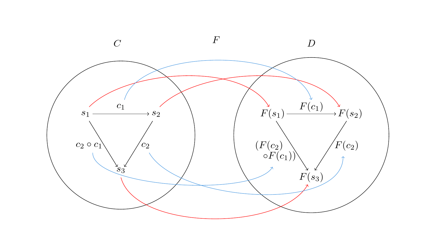
Figure 2.1: The action of a functor on a commuting diagram.

Example: Representable functors

The most fundamental type of functor is a representable functor. A functor $F:C\rightarrow\text{Set}$ from a category $C$ to Set is representable if it is naturally isomorphic to the (co- or contravariant) hom-functor, $C(c,-):C\rightarrow\text{Set}$, for some object $c$ (in which case $c$ is called the representing object). The hom-functor based at an object $c$ of the category $C$ is defined as follows: for any object $c^{\prime}\in C$, it returns the set $C(c,c^{\prime})$, of morphisms from $c$ to $c^{\prime}$; and for any morphism $g:x\rightarrow y$, it returns the function $C(c,g):C(c,x)\rightarrow C(c,y)$ between the sets $C(c,x)$ and $C(c,y)$, given by sending each element $f\in C(c,x)$ to the composite, $g\circ f$. Varying the object $c$ provides a host of perspectives on the structure of the ambient category $C$, each from the vantage point of the representing object.

2.2 The category $S^{\prime}(\mathbb{R})$

We next introduce the ‘base category’, $S^{\prime}(\mathbb{R})$, over which the Volterra series will be defined as a type of endofunctor. $S^{\prime}(\mathbb{R})$, also denoted $S^{\prime}_{\mathbb{R}}$, is the category having:

• as objects, tempered distributions (which includes the Schwartz functions; see Appendix A for a review);

• as morphisms, linear transformations that are multipliers, convolutors, or composites thereof (see Appendix A for the constructions of these maps).

The objects of $S^{\prime}(\mathbb{R})$ are signals and spectra that are ‘well-behaved’, in the sense of having convergent Fourier transforms. The morphisms are similarly well-behaved; for example, the convolutors are those maps that take Schwartz functions to Schwartz functions under convolution.

Comparison of $S^{\prime}(\mathbb{R})$ and Set

The following comparison may be useful to draw between $S^{\prime}(\mathbb{R})$ and the category Set. Whereas a set has elements, of which it is the (disjoint) union, a signal (equiv. spectrum) $s\in S^{\prime}(\mathbb{R})$ is a linear combination of its components

$$s=\sum_{r}a_{r}\boldsymbol{c}_{r},$$ (2.1)

where the vectors $\{\boldsymbol{c}_{r}\}_{r\in R}$ are elements of a frame for $S^{\prime}(\mathbb{R})$ (and if $\boldsymbol{c}_{r}(t)=e^{2\pi irt}$, then of the Fourier basis, in which case 2.1 is called a Fourier series). Whereas a function between sets maps elements to elements, a morphism $f:s\rightarrow s^{\prime}$ of signals (equiv. spectra) maps components of $s$ to components of $s^{\prime}$

$$f(s)=\sum_{i}a_{i}f_{i}(\boldsymbol{c}_{i}).$$

Now, consider the collection $S^{\prime}_{\mathbb{R}}(s_{b},s_{c})$ of morphisms between two objects, $s_{b},s_{c}\in\text{Ob}(S^{\prime}_{\mathbb{R}})$. Just as any function between sets is either injective, surjective, or bijective (i.e., both), a morphism $f\in S^{\prime}_{\mathbb{R}}(s_{b},s_{c})$ is either:

• a monomorphism: for any other object $s_{a}$ and pair of parallel arrows $g_{1},g_{2}:s_{a}\rightarrow s_{b},$ $f\circ g_{1}=f\circ g_{2}\implies g_{1}=g_{2}$

• an epimorphism: for any other object $s_{d}$ and pair of parallel arrows $g_{1},g_{2}:s_{c}\rightarrow s_{d},$ $g_{1}\circ f=g_{2}\circ f\implies g_{1}=g_{2}$

• or both (an isomorphism): $\exists f^{-1}:s_{c}\rightarrow s_{b}|f^{-1}\circ f=\text{id}_{s_{b}}$ and $f\circ f^{-1}=\text{id}_{s_{c}}.$

Restricting our attention to the epimorphisms, for example, we see that if $\text{supp}(\hat{s^{\prime}})\subset\text{supp}(\hat{s})$ (where $\text{supp}(x)$ denotes the support of $x$), then there are no convolutions in the time-domain which take $s^{\prime}$ to $s$; however, there are then infinitely many such morphisms from $s$ to $s^{\prime}$ (since any number may multiply the amplitude of any zero-amplitude frequency component without affecting the result). That said, there is a unique minimal spectral multiplier $m:\hat{s}\rightarrow\hat{s^{\prime}}$, defined by

$$m(\hat{s})[f]=\begin{cases}\frac{\hat{s^{\prime}}(f)}{\hat{s}(f)}&\hat{s^{\prime}}(f),\hat{s}(f)\neq 0\\ 0&\hat{s^{\prime}}(f)=0\end{cases};$$

and if the situation is reversed–i.e. if $\text{supp}(\hat{s})\subset\text{supp}(\hat{s^{\prime}})$–then there is a unique such minimal modulation in the time-domain (equiv. convolution in the spectral domain).

2.3 The Volterra series as a functor

We would like to exhibit the Volterra series as a kind of endofunctor, $V:S(\mathbb{R})\rightarrow S(\mathbb{R})$. For this to be true, it would have to preserve identities and composites, equivalently commuting diagrams, in $S^{\prime}(\mathbb{R})$. The action of a Volterra series $V$ on a morphism $l:s\rightarrow s^{\prime}$ is depicted

For $V$ to be a functor, the nonlinear transformation that it applies to any signal $s$ must therefore be coherent with respect to the network of relationships that $s$ has with all other signals in $S^{\prime}(\mathbb{R})$, as encoded in the morphisms between it and them. Thus, $V$ must send a morphism $f:s\rightarrow s^{\prime}$ in $S^{\prime}(\mathbb{R})$ to a linear transformation $V(f)$, also in $S^{\prime}(\mathbb{R})$, that maps components of $V(s)$ to components of $V(s^{\prime})$:

$$V(f)V(s)=\sum_{i}V_{i}(f_{i})V_{i}(s)=\sum_{i}V_{i}(f_{i})\boldsymbol{x}_{i},$$

where $\boldsymbol{x}_{i}$ is the output of the $i^{\text{th}}-$VO.

In the special case that $l$ is a LTI map, then $V(l)$ is of the form

$$V(l):V(s)\rightarrow V(s^{\prime})$$

$$V(l)(V(s))[t]=\stackrel{{\scriptstyle[}}{{j}}=0]{\infty}{\sum}\int_{\boldsymbol{\tau}_{j}\in\mathbb{R}^{j}}v_{j}(\boldsymbol{\tau}_{j})\stackrel{{\scriptstyle[}}{{r}}=1]{j}{\prod}l(s)(t-\tau_{r})d\boldsymbol{\tau}_{j}$$

$$=\stackrel{{\scriptstyle[}}{{j}}=0]{\infty}{\sum}\int_{\boldsymbol{\tau}_{j}\in\mathbb{R}^{j}}v_{j}(\boldsymbol{\tau}_{j})\stackrel{{\scriptstyle[}}{{r}}=1]{j}{\prod}\int_{\tau^{\prime}\in\mathbb{R}}l(\tau^{\prime})s(t-\tau_{r}-\tau^{\prime})d\tau^{\prime}d\boldsymbol{\tau}_{j},$$

or, in the frequency domain,

$$V(l)(V(s))[t]=\stackrel{{\scriptstyle[}}{{j}}=0]{\infty}{\sum}\,\sideset{}{{}_{\boldsymbol{\Omega}_{j}\in\mathbb{R}^{j}}}{\int}e^{i\Sigma\boldsymbol{\Omega}_{j}t}\hat{\,v_{j}}(\boldsymbol{\Omega}_{j})\,\stackrel{{\scriptstyle[}}{{q}}=1]{j}{\prod}\hat{l}(\omega_{q})\hat{s}(\omega_{q})d\boldsymbol{\Omega}_{j}.$$

$$=\stackrel{{\scriptstyle[}}{{j}}=0]{\infty}{\sum}\,\sideset{}{{}_{\boldsymbol{\Omega}_{j}\in\mathbb{R}^{j}}}{\int}e^{i\Sigma\boldsymbol{\Omega}_{j}t}\hat{\,v_{j}}(\boldsymbol{\Omega}_{j})\,\hat{l}^{\otimes j}(\boldsymbol{\Omega}_{j})\stackrel{{\scriptstyle[}}{{q}}=1]{j}{\prod}\hat{s}(\omega_{q})d\boldsymbol{\Omega}_{j},$$

where $\hat{l}^{\otimes j}$ is the $j^{\text{th}}$ tensor power of the multiplier corresponding to the LTI transformation $l$. This appears to lead to the following general formula for the spectrum of the kernel of $V(l)$ - i.e., of the distribution by which $V(s)$ is convolved:

$$\hat{V}(l)(\omega)=\sum_{\Omega_{j}|\omega_{1}+\dots+\omega_{j}=\omega}\prod_{i}^{j}\hat{l}(\omega_{i}),$$

and we conjecture that, by this definition, $V$ is functorial.

2.4 Examples of the action of a VS on a linear transformation

Operationally, we can think of the action of a Volterra series on a linear morphism $l$ between signals as answering the question ‘‘if we apply $l:s\rightarrow s^{\prime}$ before transforming nonlinearly, what is the equivalent linear transformation $V(l):V(s)\rightarrow V(s^{\prime})$ between the nonlinearly-transformed signals?’’ In theory, this means that we should be able to obtain the result of transforming $s^{\prime}$ nonlinearly by $V$, given only the morphism $l:s\rightarrow s^{\prime}$ and the result $V(s)$ of applying $V$ to $s$. In practice, this requires that we know how a Volterra series acts on linear transformations of type $l$. It is therefore useful to catalogue some of the ways that Volterra series act on elementary linear transformations, from which actions more complex transformations can then be assembled.

2.4.1 Translation (time shift)

Let $c:s\rightarrow s^{\prime}$ be the translation-by-$l$ map, given in the time-domain as $c(s)(t)=(s*\delta_{l})(t)=\int_{\tau}s(\tau)\delta(t-l-\tau)d\tau$. Then $c$ commutes with the action of a Volterra series; i.e., $V(c):V(s)\rightarrow V(s^{\prime})$ is defined by

$$V(c)V(s)(t)=V(c(s))(t)$$

$$=\sum_{j=0}^{\infty}\int_{\omega\in\mathbb{R}}e^{i\omega t}\int_{\boldsymbol{\Omega}_{j}\in\mathbb{R}^{j}|\Sigma\boldsymbol{\Omega}_{j}=\omega}\hat{v}_{j}(\boldsymbol{\Omega}_{j})\prod_{r=1}^{j}e^{-i\omega_{r}\tau}\hat{s}(\omega_{r})d\boldsymbol{\Omega}_{j}d\omega$$

$$=\sum_{j=0}^{\infty}\int_{\omega\in\mathbb{R}}e^{i\omega t}\int_{\boldsymbol{\Omega}_{j}\in\mathbb{R}^{j}|\Sigma\boldsymbol{\Omega}_{j}=\omega}e^{-i(\omega_{1}+\dots+\omega_{j})\tau}\hat{v}_{j}(\boldsymbol{\Omega}_{j})\hat{s}^{\otimes j}(\boldsymbol{\Omega}_{j})d\boldsymbol{\Omega}_{j}d\omega$$

$$=\sum_{j=0}^{\infty}\int_{\omega\in\mathbb{R}}e^{i\omega(t-\tau)}\hat{y}_{j}(\omega)d\omega$$

$$=V(s)(t-\tau),$$

where $\hat{y}_{j}$ is the spectrum of the output of the $j^{\text{th}}-$order operator, $V_{j}$.

2.4.2 Modulation (frequency shift)

Let $m:s\rightarrow s^{\prime}$, $m(s)(t)=e^{i\xi t}s(t)$ be the modulation-by-$\xi$ map. Then $V(m):V(s)\rightarrow V(s^{\prime})$ is defined by

$$V(m)V(s)(t)$$

$$=\stackrel{{\scriptstyle[}}{{j}}=0]{\infty}{\sum}\int_{\boldsymbol{\tau}_{j}\in\mathbb{R}^{j}}v_{j}(\boldsymbol{\tau}_{j})\stackrel{{\scriptstyle[}}{{r}}=1]{j}{\prod}e^{i\xi(t-\tau_{r})}s(t-\tau_{r})d\boldsymbol{\tau}_{j}$$

$$=\stackrel{{\scriptstyle[}}{{j}}=0]{\infty}{\sum}\int_{\boldsymbol{\tau}_{j}\in\mathbb{R}^{j}}e^{i\xi\Sigma(t\boldsymbol{1}-\boldsymbol{\tau}_{j})}v_{j}(\boldsymbol{\tau}_{j})s^{\otimes j}(t\boldsymbol{1}_{j}-\boldsymbol{\tau}_{j})d\boldsymbol{\tau}_{j}$$

$$=\stackrel{{\scriptstyle[}}{{j}}=0]{\infty}{\sum}e^{ij\xi t}\int_{\boldsymbol{\tau}_{j}\in\mathbb{R}^{j}}e^{-i\xi\Sigma\boldsymbol{\tau}_{j}}v_{j}(\boldsymbol{\tau}_{j})s^{\otimes j}(t\boldsymbol{1}_{j}-\boldsymbol{\tau}_{j})d\boldsymbol{\tau}_{j}$$ (2.2)

$$=\stackrel{{\scriptstyle[}}{{j}}=0]{\infty}{\sum}e^{2ij\xi t}\left(\hat{v}_{j}*e^{-i\xi t}\hat{z}^{\otimes j}\right)(\xi\boldsymbol{1}).$$

where $\hat{z}^{\otimes j}(\boldsymbol{\Omega}_{j})=\hat{s}^{\otimes j}(-\boldsymbol{\Omega}_{j})$. Note that the integral term in (2.2) is exactly the multidimensional short-time Fourier transform (STFT), $Q_{v_{j}}(s^{\otimes j})$, of the signal tensor, $s^{\otimes j}$, with window function the VKF, $v_{j}$, evaluated at the pair consisting of the constant-$\xi$ frequency and constant-$t$ vectors. Thus, (2.2) can be written

$$=\sum_{j}e^{ij\xi t}Q_{v_{j}}(s^{\otimes j})(\xi\boldsymbol{1},t\boldsymbol{1}).$$ (2.3)

If the input $s$ is the constant unity signal $\boldsymbol{1}$, then (2.3) reduces to the response of a Volterra series to a pure complex exponential input (see: [5], Section 2.4; or [6]):

$$V(m)V(\boldsymbol{1})(t)=\sum_{j}e^{ijt\xi}\,\hat{v}_{j}(\xi\boldsymbol{1}).$$

2.4.3 Periodization

See (Appendix A, Sect. A.2) for background on the Dirac comb and its tensor products.

Let $c:s\rightarrow s^{\prime}$ be the operation of convolution against the Dirac comb with period $T$: $c(s)(t)=(\text{Ш}_{T}*s)(t)$; such an operation ‘periodizes’ the signal $s$. Then $V(c):V(s)\rightarrow V(s^{\prime})$ is defined by

$$V(c)V(s)(t)=V(c(s))(t)$$

$$=\sum_{j=0}^{\infty}\int_{\omega\in\mathbb{R}}e^{i\omega t}\int_{\boldsymbol{\Omega}_{j}\in\mathbb{R}^{j}|\Sigma\boldsymbol{\Omega}_{j}=\omega}\hat{v_{j}}(\boldsymbol{\Omega}_{j})\prod_{r=1}^{j}\text{Ш}_{\frac{1}{T}}(\omega_{r})\hat{s}(\omega_{r})d\boldsymbol{\Omega}_{j}d\omega$$

$$=\sum_{j=0}^{\infty}\int_{\omega\in\mathbb{R}}e^{i\omega t}\int_{\boldsymbol{\Omega}_{j}\in\mathbb{R}^{j}|\Sigma\boldsymbol{\Omega}_{j}=\omega}\hat{v_{j}}(\boldsymbol{\Omega}_{j})\,\text{Ш}_{\frac{1}{T}}{}^{\otimes j}(\boldsymbol{\Omega}_{j})\hat{s}^{\otimes j}(\boldsymbol{\Omega}_{r})d\boldsymbol{\Omega}_{j}d\omega$$

$$=\sum_{j=0}^{\infty}\int_{\omega\in\mathbb{R}}e^{i\omega t}\sum_{\boldsymbol{k}\in\mathbb{Z}^{j}\,|\,\Sigma T^{-1}\boldsymbol{k}=\omega}\hat{v_{j}}(T^{-1}\boldsymbol{k})\hat{s}^{\otimes j}(T^{-1}\boldsymbol{k})d\omega$$

which, collecting multicombinations of integer indices $k_{i}\in\mathbb{Z}$ making up the vector $\boldsymbol{k}=[\overbrace{k_{1},\dots,k_{1}}^{n(k_{1})};\dots;\overbrace{k_{p},\dots,k_{p}}^{n(k_{p})}]$, and counting permutations of these multicombinations, can be rewritten

$$=\sum_{j=0}^{\infty}\int_{\omega\in\mathbb{R}}e^{i\omega t}\sum_{\boldsymbol{k}|\Sigma T^{-1}\boldsymbol{k}=\omega}\binom{j}{n(k_{1}),\dots,n(k_{p})}\,\hat{v_{j}}(T^{-1}\boldsymbol{k})\,\hat{s}^{\otimes j}(T^{-1}\boldsymbol{k})d\omega.$$ (2.4)

2.4.4 Sampling

Let $m:s\rightarrow s^{\prime}$ be the operation of multiplication against the Dirac comb with period $T$: $m(s)(t)=(\text{Ш}_{T}\cdot s)(t)$ ; such an operation ‘samples’ the signal $s$. Then $V(m):V(s)\rightarrow V(s^{\prime})$ is defined

$$V(m)V(s)(t)=V(m(s))(t)$$

$$=\stackrel{{\scriptstyle[}}{{j}}=0]{\infty}{\sum}\int_{\boldsymbol{\tau}_{j}\in\mathbb{R}^{j}}v_{j}(\boldsymbol{\tau}_{j})\stackrel{{\scriptstyle[}}{{r}}=1]{j}{\prod}\text{Ш}_{T}(t-\tau_{r})s(t-\tau_{r})d\boldsymbol{\tau}_{j}$$

$$=\stackrel{{\scriptstyle[}}{{j}}=0]{\infty}{\sum}\int_{\boldsymbol{\tau}_{j}\in\mathbb{R}^{j}}v_{j}(\boldsymbol{\tau}_{j})\,\text{Ш}_{T}{}^{\otimes j}(t\boldsymbol{1}_{j}-\boldsymbol{\tau}_{j})\,s^{\otimes j}(t\boldsymbol{1}_{j}-\boldsymbol{\tau}_{j})d\boldsymbol{\tau}_{j}$$

$$=\sum_{j=0}^{\infty}\,\,\sum_{\boldsymbol{k}\in\mathbb{Z}^{j}|\,\Sigma n(k_{i})=j}\binom{j}{n(k_{1}),\dots,n(k_{p})}\,v_{j}(t\boldsymbol{1}-T\boldsymbol{k})\,s^{\otimes j}(t\boldsymbol{1}-T\boldsymbol{k})$$ (2.5)

where $\boldsymbol{k}=[\overbrace{k_{1},\dots,k_{1}}^{n(k_{1})};\dots;\overbrace{k_{p},\dots,k_{p}}^{n(k_{p})}]$, as in example 2.4.3.

If the input is the constant unity signal, $\boldsymbol{1}$, then (2.5) reduces to the result known for the response of a Volterra series to a combination of impulsive inputs ([5], Section 5.1), specialized to the case where the inputs are spaced at regular intervals of length $T$:

$$V(\text{Ш}_{T})(t)=\sum_{j=0}^{\infty}\,\,\sum_{\boldsymbol{k}\in\mathbb{Z}^{j}|\,\Sigma n(k_{i})=j}\binom{j}{n(k_{1}),\dots,n(k_{p})}\,v_{j}(t\boldsymbol{1}-T\boldsymbol{k}).$$

In each of the above examples, the result of nonlinearly processing the linearly transformed signal is represented as a sum of linearly transformed homogeneous outputs. As the homogeneous outputs $V_{j}(s)$ form a frame for a certain subspace of $S(\mathbb{R})$ (in which the output $x(t)$ is given by their unweighted linear combination), the sum of linearly transformed homogeneous outputs can always be rewritten using a frame transformation as a single linear transformation of the total output: $V(f(s))(t)=V(f)x(t)$.

Chapter 3 The category of Volterra series

No system that exists in the physical world remains forever the same; rather, its identity, the particular way that it processes signals, inevitably changes with time. Such a system is called nonstationary, in contrast to (an idealized) one whose response pattern is invariant with respect to its inputs or past. For example, a linear translation-invariant system is nonstationary if its impulse response is time-varying. Likewise, we call a nonlinear system represented by a Volterra series nonstationary if any of its VKFs (or higher order impulse response functions) vary.

Nonstationarity, as a concept, provides a context for questions such as: which parts of a system are changing, and in which ways, and how fast? The stability of identity becomes a property to be modeled and measured. Like nonlinearity, however, nonstationarity is a negativistic property. Knowing, in principle, that a system changes does not tell us how it does so. For example, in section (1.3), we briefly reviewed a form of parametricity for Volterra series that was, as described, apparently achieved simply by formally adjoining a scalar variable upon which certain terms in the Volterra series were made to depend; yet, the mechanism by which that dependancy had been introduced was not, itself, made clear.

In this chapter, we introduce the notion of a morphism of Volterra series, which models a change in the response pattern of a nonlinear system. We do so by defining a Volterra series morphism $\phi:V\rightarrow W$ as a kind of lens map, which consists of a pair, $(\phi_{1},\phi^{\#})$, of functions, namely: a function $\phi_{1}$, between the index-sets of the series; and, for each pair of indices $(i,\phi_{1}(i))$, a dependent linear map $\phi_{i}^{\#}:S^{\prime}(\mathbb{R}^{[\phi_{1}(i)]})\rightarrow S^{\prime}(\mathbb{R}^{[i]})$ between the function spaces of their respective kernels. We also conjecture that such maps are natural transformations, having previously conjectured that the Volterra series is a type of functor. Equipped with Volterra series morphisms, we then define a category, the category of Volterra series. Before beginning, however, we first recall the notion of natural transformation.

3.1 Natural transformations

Just as functors are structure-preserving maps between categories, natural transformations are structure-preserving maps between functors. Given two functors $F,G:C\rightarrow D$, a natural transformation $\alpha:F\rightarrow G$ consists of a collection of components, $\alpha_{(-)}\in\text{Mor}(D),$ indexed by the objects of $C$. These components must satisfying the following condition: for any morphism $f:x\rightarrow y$ in $C$, the square

commutes in $D$; i.e., $\alpha_{y}(F(f)(F(x)))=G(f)(\alpha_{x}(F(x))$. A natural transformation $\alpha:F\rightarrow G$ may also be denoted

to emphasize the fact that, being as it is a morphism between functors, it is ‘two-dimensional’, or a $2-$ morphism.

Example: Transformation between Representable functors $S(\mathbb{R})\rightarrow\text{Set}$

Recall the notion of representable functor from Section 2.1. Let $y^{S},y^{S^{\prime}}:S(\mathbb{R})\rightarrow\text{Set}$ be two (Set-valued) functors on $S(\mathbb{R})$, represented at the objects $s$ and $s^{\prime}$, respectively. Given any morphism $f:s^{\prime}\rightarrow s$, there is an induced natural transformation, $\alpha$, as follows: for any other morphism $h:A\rightarrow B$ between objects $A,B\in S(\mathbb{R})$, the component of $\alpha$ at $A$ (resp. $B$) is given by precomposition with $f$: $\alpha_{A}(g)=g\circ f$, where $g\in A^{S}$. The following diagram then commutes

since $h\circ\alpha_{a}(g)=h\circ(g\circ f)=(h\circ g)\circ f=\alpha_{b}(h\circ g)$, by the associativity of composition of linear maps.

3.2 Morphisms of Volterra series

The data of a natural transformation between functors whose domains are both a category like Set, or $S^{\prime}(\mathbb{R})$, whose collection of objects is infinite, is in theory specified by an infinite number of commuting diagrams. As in the above example, however, it may be possible to specify a rule (which in the example was given by precomposition with the map $f$) that causes all of the diagrams to commute. We will define morphisms of Volterra series via such a rule, shortly; but first, a notational remark must be made.

Notational aside: index sets and nonlinear orders

A Volterra series is often assumed to consist of a single homogeneous operator at each order of nonlinearity, as reflected by the indexing variable $j\in\mathbb{N}$ in the left-most sum of the defining equation (1.2). However, in Chapter 4 we will describe ways of combining Volterra series that result in series which contain multiple homogeneous operators of the same order of nonlinearity; we therefore need to be able to distinguish homogeneous operators of similar order.

Let $I_{V}$ or just $I\in\text{Ob(Set)}$ denote the index-set of the homogeneous operators in a Volterra series $V$, and let $i\in I$ be such an index. Then, in certain contexts that will be made clear, we will write $[i]$ for the order of nonlinearity of the homogeneous operator indexed by $i$. Thus, for example, if $[i]=j$, then the VKF at at index $i$ has type $v_{i}:\mathbb{R}^{j}\rightarrow\mathbb{R}$ (modulo symmetry and any other constraints).

In the special case that the magnitude of the $0^{\text{th}}-$frequency component of every homogeneous operator in a Volterra series $V$ is $1$, then an elegant way of generating the index-set of $V$ is to have $V$ operate on the constant input $\boldsymbol{1}$: $I_{V}\cong V(\boldsymbol{1})$. We will make this assumption (that $I_{V}\cong V(\boldsymbol{1})$) at times in what follows, and use the notation $V(\boldsymbol{1})$ to refer to the index set of the homogeneous operators in a series.

3.2.1 Morphisms as lens maps

The definition we are about to give of a morphism of Volterra series is an example of what is known in category theory and computer science as a lens. In the category Set, a (dependent) lens $\binom{\phi_{1}}{\phi_{(-)}^{\#}}$$:(A\times B)\rightarrow(C\times D)$ is comprised of: a map $\phi_{1}:A\rightarrow C$; and for each $a\in A$, a dependent function $\phi_{a}^{\#}:A\times D\rightarrow B$. This lens construction is used in [55] to define morphisms between polynomial functors, which are functors Set$\rightarrow$Set that are given as sums (coproducts) of representable functors. Adapting the lens construction to work for Volterra series results in the following definition.

Definition:

A morphism $\phi:V\rightarrow W$ of Volterra series is comprised of the following data:

• a function $\phi_{1}:I_{V}\rightarrow I_{W}$ between index-sets;

• for each pair $(i,\phi_{1}(i))$, with $i\in I_{V}$ and $\phi_{1}(i)\in I_{W}$,

  • a linear map $\phi_{i}^{\#}:S(\mathbb{R}^{[\phi_{1}(i)]})\rightarrow S(\mathbb{R}^{[i]})$ between the function spaces of their respective kernels.

That is, for each homogeneous operator $V_{i}$ of the series $V$, we choose a homogeneous operator $W_{\phi_{1}(i)}$ of the series $W$; then we choose a contravariant linear map back, from the function space $W_{\phi_{1}(i)}$ to the function space of $V_{i}$. Once these components have been determined, and writing $k=\phi_{1}(i)$ for the index of the homogeneous operator in $W$ corresponding to the index $i$ in $V$, the image $\phi(V_{i}(s))$ for any homogeneous output $V_{i}(s)$ under the morphism $\phi$ is defined

$$\phi(V_{i}(s))(t)=$$

$$\int_{\boldsymbol{\tau}_{[i]}\in\mathbb{R}^{[i]}}v_{i}(\boldsymbol{\tau}_{[i]})\,\left(\phi_{i}^{\#}(w_{\phi_{1}(i)}*s^{\otimes[\phi_{1}(i)]})\right)(t\boldsymbol{1}-\boldsymbol{\tau}_{[i]})\,d\boldsymbol{\tau}_{[i]}=$$ (3.1)

$$(v_{i}*(\phi_{i}^{\#}(w_{k}*s^{\otimes[k]}))[t\boldsymbol{1}].$$

Geometrically and operationally, equation (3.1) says that, for each homogeneous operator $V_{i}$ of the source series, a delegate is chosen from amongst the homogeneous operators of the target series - i.e., the pair $(i,\phi_{1}(i))$ is formed. An interface is next created via the map $\phi^{\#}$ , and a composition of filtering operations is then carried out via the interface: first, the input tensor is convolved with $w_{\phi_{1}(i)}$, and then its image under $\phi_{i}^{\#}$ is convolved with $v_{i}$. Finally, the output is obtained by indexing the resulting multidimensional signal along its diagonal, $t\boldsymbol{1}$.

The following morphisms exist for any Volterra series:

Trivial Morphism

The trivial morphism $\alpha:V\rightarrow(\sum_{j}(\delta^{\otimes j}))$ is the morphism with target the series whose VKF at each order $j$ is a multidimensional distribution centered at the origin, and whose maps $\phi_{1}$ and $\phi^{\#}$ are both the identity maps.

Autoconvolution

The autoconvolution $\text{aut}_{V}:V\rightarrow V$ is given by the pair $(\phi_{1},\phi^{\#})$, where both $\phi_{1}$ and all of the $\phi_{i}^{\#}$ are identity maps. This map results in the Volterra series whose VKF at each order $i$ is the autoconvolution $(v_{i}*v_{i})$ of $v_{i}$.

Identity morphism

The identity morphism $\text{id}_{V}:V\rightarrow V$ is given by the pair $(\phi_{1},\phi^{\#})$, where $\phi_{1}=\text{id}_{V(\boldsymbol{1})}$ is the identity and where, for any $i\in V(\boldsymbol{1})$, $\phi_{i}^{\#}:S^{\prime}(\mathbb{R}^{[i]})\rightarrow S^{\prime}(\mathbb{R}^{[i]})$ is the unique linear map that scales by the reciprocal of the spectrum of $v_{i}$, i.e. $\phi_{i}^{\#}(\hat{x})(\boldsymbol{\Omega})=\frac{\hat{x}(\boldsymbol{\Omega})}{\hat{v}_{i}(\boldsymbol{\Omega})}$ for $\hat{v}_{i}(\boldsymbol{\Omega})\neq 0$. The definition of $\phi_{i}^{\#}$ follows from the fact that the spectrum of the autoconvolution $R_{v_{i}}=(v_{i}*v_{i})$ is $\hat{R}_{v_{i}}(\boldsymbol{\Omega}_{[i]})=\hat{v}_{i}(\boldsymbol{\Omega}_{[i]})^{2}$.

3.2.2 Parameterized morphisms

Morphisms of Volterra series can also be parameterized by one or many real variables. Each of the following examples of this corresponds to a well-known operation in signal processing, and provides a basic template by which a parameterized family of Volterra series can be generated in a continuous fashion.

Translation

Let $\boldsymbol{\tau}=[\tau_{1},\boldsymbol{\tau}_{2},\dots,\boldsymbol{\tau}_{j}]\in\mathbb{R}\times\mathbb{R}^{2}\times\dots\times\mathbb{R}^{j}$; then the translation-by-$\boldsymbol{\tau}$ morphism is the morphism with target the VS whose VKF at each order $i$ is a multidimensional distribution centered at $\boldsymbol{\tau}_{i}$, with $\phi_{1}=\text{id}$ and all of the $\phi_{i}^{\#}$ also identities. The offsets can be varied and/or the morphism iterated.

Sampling

Similarly, sampling corresponds to a morphism $V\rightarrow\sum_{j}W_{j}$, where the VKF of the target series at order $j$ is given by multiplication against a Dirac comb, $w_{j}(\boldsymbol{\tau}_{j})=\text{\leavevmode{Ш}}(\boldsymbol{\tau}_{j})$. The period $T_{j}$ of the comb at order $j$ can be varied.

Smoothing

Smoothing corresponds, in one example, to a morphism $V\rightarrow(\sum_{j}W_{j})$ where the VKFs of the target series are normal distributions, i.e. $w_{j}(\boldsymbol{\tau}_{j})=e^{-\boldsymbol{\tau}_{j}^{\top}C_{j}\boldsymbol{\tau}_{j}}$ and $C_{j}$ is a positive-definite $j\times j$ matrix. The morphism can be iterated. Similarly, a target series whose VKFs are the stencils of Laplacian operators can be used to drive diffusion.

Other morphisms, which might, for example, affect transformations such as periodization or shearing can be similarly defined (possibly via composition with a Fourier transform).

3.2.3 Naturality of Volterra morphisms

In section 2.3, we conjectured that the Volterra series is a functor. In that case, we should expect that morphisms of Volterra series are natural transformations. For that to be so, squares of the form

for $s,s^{\prime}\in S^{\prime}(\mathbb{R})$ and $f:s\rightarrow s^{\prime}$, must commute.

Suppose that the Volterra series is a functor, and let the components of a mapping between two Volterra series $V$ and $W$ be defined by

$$\alpha_{s}(V(s))=\sum_{j}\text{diag}((v_{j}*-)\circ(\phi_{j}^{\#}(w_{\phi_{1}(j)}*-))(s^{\otimes[\phi_{1}(j)]})$$

$$=\sum_{j}\text{diag}(v_{j}*(\phi_{j}^{\#}(w_{\phi_{1}(j)}*s^{\otimes[\phi_{1}(j)]}))).$$

where $\alpha_{s}(V(s))\in W(s)$. Since morphisms of VS leave the input signal tensor unchanged and Volterra series act on morphisms of signals by precomposition, naturality should follow by a similar logic to that in example 3.1.1; i.e., we have

$$W_{f}\circ\alpha_{s}=W(f)(\alpha_{s}(V(s))=\alpha_{f(s)}(V(f)V(s))=\alpha_{s^{\prime}}V(s^{\prime}).$$

3.3 Volterra series form a category

Given any category $C,$ and any endofunctor $F:C\rightarrow C$, there is an identity natural transformation, denoted $1_{F}$. Furthermore, natural transformations compose associatively. Thus, for any category $C$, there is a functor category whose objects are endofunctors on $C$ and whose morphisms are natural transformations between them.

However, as we only conjectured that the Volterra series is a type of functor, we will instead show that Volterra series form a category when the morphisms between them are considered as lens maps. Recall from 3.2.1 that the identity morphism at any Volterra series $V$ can be construction represented as a lens map; so, it remains to address the composition of Volterra series morphisms. For any three Volterra series $V,W,Z$, and morphisms $f,g,h$ between them as shown, the diagram:

commutes iff the following two diagrams describing the corresponding lens maps do:

This is the case when $h_{1}=g_{1}\circ f_{1}$ and $h_{i}^{\#}=g_{f_{1}(i)}^{\#}\circ f_{i}^{\#}$. As functions between sets and linear maps between function spaces compose associatively, so do the components $\phi_{1}$ and $\phi_{(-)}^{\#}$ of any Volterra morphism construed as a lens map $\phi$. We can now give the following definition:

Definition:

The category, Volt, of Volterra series is the category having, as objects, Volterra series, and as morphisms, morphisms of Volterra series, considered as lens maps.

It follows that the initial object in Volt is the empty Volterra series, $0$; i.e., for any other Volterra series $V$, $|\text{Volt}(0,V)|=1$, where the unique element of the hom-set $\text{Volt}(0,V)$ is the morphism that vacuously sends every homogeneous operator in $0$ (of which there are none) to a homogeneous operator in $V$, and is nullary on morphisms. Conversely, the terminal object in Volt is the constant Volterra series, $V_{0}=1$.

In Chapter 4, we study three ways of combining Volterra series, each of which has the form of a monoidal product, $(-\diamond-):\text{\emph{Volt}$\times$\emph{Volt}$\rightarrow\emph{Volt}$}$. By working not, merely, with the set of all Volterra series, but rather with Volterra series and their morphisms in concert, it becomes possible and, indeed, natural to study the associated universal properties of these operations. This is fundamentally because morphisms of Volterra series provide a means of describing how Volterra series transform, not in isolation, but functionally and in relation to one another.

Chapter 4 Volt as a monoidal category

The modeling of complex systems as interconnections and compositions of simpler ones, be it via a synthetic or an analytic approach to the problem, is a hallmark of scientific methodology. However, representing a complex system merely as an interconnection may bring little benefit if the rules for interconnection and the properties of those rules are not well understood. This understanding constitutes the difference between mere modularity and compositionality. Whereas, in a modular paradigm, one is able to arrange systems and interconnect them but might not know how the various interconnections are related, in a compositional paradigm one has access, in the form of equivalences or isomorphisms, to knowledge of this kind. Category-theoretically, such equivalences are encoded in the axioms of a monoidal category.

The need for a modular and compositional theory is especially poignent when it comes to nonlinear systems, since a nonlinear system’s complexity grows quickly with its order of nonlinearity. For example, in nonlinear system identification, harmonic probing methods for the estimation of Volterra series parameters have an algorithmic complexity that, in their naive formulation, grows exponentially in the system memory and order of nonlinearity, which limits their usefullness in identifying Volterra series that are represented monolithically. Modeling a complex nonlinear system instead as a composition of lower-order Volterra series in theory enables the parameters of the simpler series to first be estimated separately, and then the results to be combined using the interconnection rules. In such cases, beyond the benefit brought by mere modularity, compositionality further provides the ability to flexibly rearrange the component subsystems – for example, to re-associate them in series – without requiring the reestimation of their parameters. Compositionality stands, dually, to bring the same kind of benefit to the synthesis, rather than the analysis, of complex nonlinear systems.

Modularity and compositionality are furthermore idiomatic to the domain of audio. From the design of a modular synthesizer, to the orchestration of an ensemble, to the composition of a musical score, to the performance of a musical piece, musicians, composers, instrument designers, and audio engineers regularly rearrange and interconnect nonlinear systems, and do so in a rich variety of ways - intuitive, experimental, and theoretical. What is more, these musical acts and practices are often carried out live, or in real-time.

Our goal in this chapter is to place upon category-theoretic foundations a compositional theory of nonlinear audio systems and their transformations, as modeled by Volterra series and their morphisms. We do this by studying three core operations - following closely the analogous parts of the exposition in [55] - each of which has the form of a bifunctor on the category Volt, and show how each satisfies a corresponding universal property. As the culmination of our efforts, we show that Volt is a monoidal category under the operation of series composition. We begin by recalling the notion of monoidal category.

4.1 Monoidal categories

A monoidal category is a category $C$ equipped with:

• a bifunctor

  $$\diamond:C\times C\rightarrow C,$$

  also called the monoidal (or tensor) product, that is associative up to a natural isomorphism;

• an object, $I$, called the monoidal unit, that acts as both a left and right identity for $\diamond$, up to natural isomorphism;

• and natural isomorphisms:

  • the associator: $\mathfrak{a}:((-)\diamond(-))\diamond(-)\stackrel{{\scriptstyle\cong}}{{\rightarrow}}(-)\diamond((-)\diamond(-)),\,\mathfrak{a}_{x,y,z}:(x\diamond y)\diamond z\rightarrow x\diamond(y\diamond z)$

  • the left and right unitors:

$\begin{array}[]{cccc}\lambda:(1\diamond(-))\stackrel{{\scriptstyle\cong}}{{\rightarrow}}(-)&&&\rho:((-)\diamond 1)\stackrel{{\scriptstyle\cong}}{{\rightarrow}}(-)\\ \lambda_{x}:1\diamond x\rightarrow x&&&\rho_{x}:x\diamond 1\rightarrow x\end{array}$

such that the following diagrams commute:

triangle identity

pentagon identity

The notion of monoidal category is a categorification of that of monoid, which is a category having only one object. See [60] for an introduction to monoidal category theory and a tour of various examples of monoidal categories. Examples of monoidal categories include: the category Vect of vector spaces and linear maps, with monoidal product the ordinary tensor product; and the category Set, equipped with either the disjoint union or the Cartesian product as the monoidal product.

To any monoidal category there is furthermore associated a diagrammatic language, whose terms are known as string diagrams, in which applying the tensor product corresponds to putting morphisms in parallel, and regular composition to putting them in series. Such a language is resemblant of wiring diagrams in electrical engineering and signal flow graphs in signal processing, but is fully formal, meaning that topological deformations of the diagrams correspond to known algebraic manipulations; see [61] for a comprehensive overview of the various string diagrammatic languages corresponding to different monoidal categories.

4.2 Sum and product of Volterra series

Sum (coproduct)

What happens when the outputs of two Volterra series that process the same input signal are added? Can we represent the result using a single series? Indeed, the sum $V+W$ of two Volterra series is defined simply by the level-wise addition of their homogeneous operators; equivalently, of the VKFs of the same order

$$(V+W)(s)(t)$$

$$=\sum_{j}(V+W)_{j}(s)(t)=\sum_{j}V_{j}(s)(t)+W_{j}(s)(t)$$

$$=\int_{\boldsymbol{\tau}_{j}\in\mathbb{R}^{j}}(v_{j}(\boldsymbol{\tau}_{j})+(w_{j}(\boldsymbol{\tau}_{j}))\prod_{q=0}^{j}s(t-\tau_{q})d\boldsymbol{\tau}_{j}$$

where the last line follows by linearity.

While this operation is well-known in the Volterra series literature, we would like to show that it is, category-theoretically, the coproduct in the category Volt; i.e., that it satisfies the following universal property. Let $\iota,\kappa$ denote the inclusions of $V$ and $W$ into $V+W$. Then given any other Volterra series $X$ and any pair of morphisms $f,g$ where $f:V\rightarrow X$ and $g:W\rightarrow X$, there is a unique morphism $h:V+W\rightarrow X$ making the following diagram commute:

Recall from section 3.3 that, by representing the morphisms $f,g,\iota,\kappa$, and $h$ as lens maps, this is equivalent to requiring the commutation both of: (1) a diagram of maps between the index sets of the homogeneous operators of the series, and; (2) a diagram of maps between their respective function spaces. The first of these conditions states that the diagram

must commute; i.e., $h_{1}$ is the function which sends each $(1,i)\in V(\boldsymbol{1})+W(\boldsymbol{1})$, where $i\in V(\boldsymbol{1})$, to $f_{1}(i)$, and each $(2,j)\in V(\boldsymbol{1})+W(\boldsymbol{1})$, where $j\in W(\boldsymbol{1})$, to $g_{1}(j)$. This diagram is the standard one for the coproduct of sets.

For the diagram of the maps between function spaces, we obtain:

But both $\iota_{i}^{\#}$ and $\kappa_{j}^{\#}$ are identities, so we must have that $h_{(1,i)}^{\#}=f_{i}^{\#}$ and $h_{(2,j)}^{\#}=g_{j}^{\#}.$ Since both sets of diagrams commute, so does the original.

Product

What happens if the outputs of two Volterra series that process the same signal are multiplied? Can we express the result as the output of a single series? Indeed, the product $V=A\times B$ of two Volterra series $A$ and $B$ is given by the formula [29, 5]

$$V(s)(t)=(A\times B)(s)(t)$$

$$=\sum_{j}\sum_{k=0}^{j}(A_{k}(s)B_{j-k}(s))(t)$$ (4.1)

which can be rewritten

$$\begin{array}[]{c}V_{j}(s)(t)=\sum_{k=0}^{j}\sideset{}{{}_{\Omega_{k}\in\mathbb{R}^{k}}}{\int}e^{i\Sigma\Omega_{k}t}\hat{a}_{k}(\Omega_{k})\stackrel{{\scriptstyle[}}{{p}}=0]{k}{\prod}\hat{s}(\omega_{p})d\omega_{p}\\ \times\sideset{}{{}_{\Omega_{j-k}\in\mathbb{R}^{j-k}}}{\int}e^{i\Sigma\Omega_{j-k}t}\hat{b}_{j-k}(\Omega_{j-k})\stackrel{{\scriptstyle[}}{{q}}=0]{j-k}{\prod}\hat{s}(\omega_{q})d\omega_{q}.\end{array}$$ (4.2)

The above can be further rewritten under a single integral using an index notation similar to that from section $1.2$. Let $\theta_{1}^{p},\theta_{2}^{p},...,\theta_{k}^{p}$, with $\theta_{i}^{p}\in\mathbb{R}^{\alpha_{i}^{p}}$, be a sequence of vectors that partition (into parts of possibly zero size) the vectorial frequency variable $\Omega_{j}$, where the superscript $p$ indicates a given $k-$multicomposition of $j$; i.e., whose lengths

$$\alpha_{i}^{p}\geq 0,\,\,(i=1,2)$$

are such that

$$\stackrel{{\scriptstyle[}}{{i}}=1]{k}{\sum}\alpha_{i}^{p}=j.$$

In the case of the binary product - i.e., where $k=2$ - eq. (4.2) can be rewritten as

$$V_{j}(s)(t)=\sum_{p=1}^{\binom{j+1}{j}}\sideset{}{{}_{\Omega_{j}\in\mathbb{R}^{j}}}{\int}e^{i\Sigma\Omega_{j}t}\,\widehat{a}_{\alpha_{1}^{p}}(\theta_{1}^{p})\widehat{b}_{\alpha_{2}^{p}}(\theta_{2}^{p})\prod_{r=1}^{j}\widehat{s}(\omega_{r})d\omega_{r}$$

where the binomial coefficient, $\binom{j+1}{j}=j$, counts the number of possible binary partitions of $\Omega_{j}$. Thus, the $j^{\text{th}}-$order VFRF for the composite series is

$$\widehat{v}_{j}(\Omega_{j})=\sum_{p=1}^{\binom{j+1}{j}}\widehat{a}_{\alpha_{1}^{p}}(\theta_{1}^{p})\,\,\widehat{b}_{\alpha_{2}^{p}}(\theta_{2}^{p}).$$ (4.3)

The binomial structure of the product can be seen reflected in the wiring diagram of Fig. 4.1, of a product of two series up to order $3$.

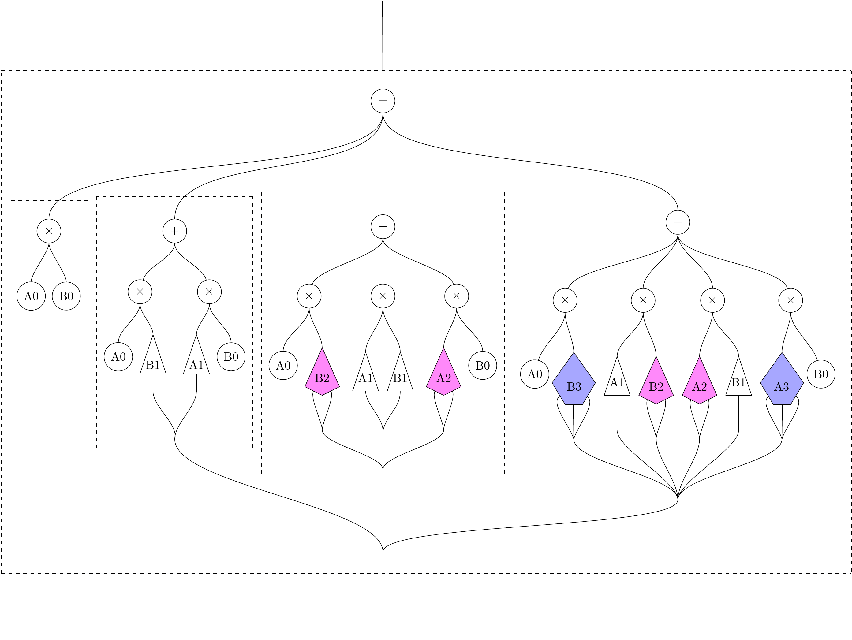
Figure 4.1: Product of Volterra series. The interior dashed boxes represent the composite homogeneous Volterra operators of the product series $A\times B$.

Just as we showed that the sum of Volterra series is indeed a categorical coproduct in Volt, so would we like to show that the product of Volterra series is the categorical product. First, let $\pi:A\times B\rightarrow A$ and $\varphi:A\times B\rightarrow B$ denote the projections out of the product and onto the factors. Then, in order for $A\times B$ to be the categorical product, the following diagrams must commute:

As with the coproduct, the commutation of a diagram of morphisms of Volterra series as natural transformations is equivalent to that of a pair of diagrams in which the morphisms are represented as lens maps. Thus, the index-level diagram

must commute. Since $\pi_{1}$ and $\varphi_{1}$ are projections, we must have that $h_{1}(k)=(f_{1}(k),g_{1}(k))$. Similarly, the diagram

of linear transformations between function spaces must commute. But as $\pi_{(f_{1}(k),g_{1}(k))}^{\#}:S^{\prime}(\mathbb{R}^{[f_{1}(k)]})\rightarrow S^{\prime}(\mathbb{R}^{[f_{1}(k)]})\oplus S^{\prime}(\mathbb{R}^{[g_{1}(k)]})\,$ and $\,\varphi_{(f_{1}(k),g_{1}(k))}^{\#}:S^{\prime}(\mathbb{R}^{[g_{1}(k)]})\rightarrow S^{\prime}(\mathbb{R}^{[f_{1}(k)]})\oplus S^{\prime}(\mathbb{R}^{[g_{1}(k)]})$ are inclusions into the coproduct (disjoint union) of function spaces, it follows that there is a unique bilinear map $h_{k}^{\#}$ such that this is so. Noting that the expression of the kernel function for the $j^{\text{th}}$ homogeneous operator in (4.3) is exactly the tensor product of the kernel functions of the factors, it thus follows that there is a unique linear map out of the tensor product, $h_{k}^{\#}:S^{\prime}(\mathbb{R}^{[f_{1}(k)]})\otimes S^{\prime}(\mathbb{R}^{[g_{1}(k)]})\rightarrow S^{\prime}(\mathbb{R}^{[k]})$.

4.3 Series Composition

The series composition, $V=B\triangleleft A$, of two Volterra series $A$ and $B$, in which the output of $A$ flows to the input of $B$ is defined on a signal $u$ by summing the outputs of all the multilinear Volterra operators of $B$ whose $k-$many inputs have orders summing to $j$; i.e.,

$$V(u)=\stackrel{{\scriptstyle[}}{{k}}=0]{n_{B}}{\sum}\underset{p|\stackrel{{\scriptstyle[}}{{r}}=1]{k}{\sum}\alpha_{r}^{p}=j}{\sum}B_{k}[y_{\alpha_{1}^{p}},\dots,y_{\alpha_{k}^{p}}]$$ (4.4)

where: $n_{B}$ is the maximum order of the series $B$; the inner sum runs over all $k-$multicompositions of $j$; and $y_{r}$ denotes the $r^{\text{th}}-$order output of $A$. Note that the second series in the composition, denoted $B$ in equation (4.4), is multivariate since, in general, many outputs from amongst the homogeneous operators of $A$ are used to compose the signals of appropriate order that are fed as inputs to the homogeneous operators of $B$.

A composite series $V=B\triangleleft A$ is given in terms of its Volterra frequency response functions[29, 30, 5] by

$$v_{j}(\boldsymbol{\Omega}_{j})=\stackrel{{\scriptstyle[}}{{k}}=0]{n_{B}}{\sum}\underset{\{p|\stackrel{{\scriptstyle[}}{{r}}=1]{k}{\sum}\alpha_{r}^{p}=j\}}{\sum}\widehat{b}_{k}(S_{p}^{(j,k)}\boldsymbol{\Omega}_{j})\stackrel{{\scriptstyle[}}{{r}}=1]{k}{\prod}\widehat{a}_{\alpha_{r}^{p}}(\boldsymbol{\theta}_{r}^{p})$$ (4.5)

where $S_{p}^{(j,k)}$ is the $j\times k$ matrix:

$$\begin{bmatrix}\overbrace{1,1,...,1}^{\alpha_{1}^{p}}&&&0\\ &\overbrace{1,1,...,1}^{\alpha_{2}^{p}}\\ &&\ddots\\ 0&&&\overbrace{1,1,...,1}^{\alpha_{k}^{p}}\end{bmatrix},$$

$\boldsymbol{\Omega}_{j}\in\mathbb{R}^{j}$ is the vector of frequency variables, and $\alpha_{r}^{p}$ are the numbers representing the lengths of the corresponding vectors in a partition, $[\theta_{1}^{p},\theta_{2}^{p},...,\theta_{k}^{p}]$ of $\boldsymbol{\Omega_{j}}$.

The composition operator, $\triangleleft$, is noncommutative, so it induces an (temporal) ordering of its operands. The binary composition of two series, up to order $3$ and with the $0^{\text{th}}-$order operator $A_{0}$ assumed equal to $0$, is shown in Fig. 4.2.

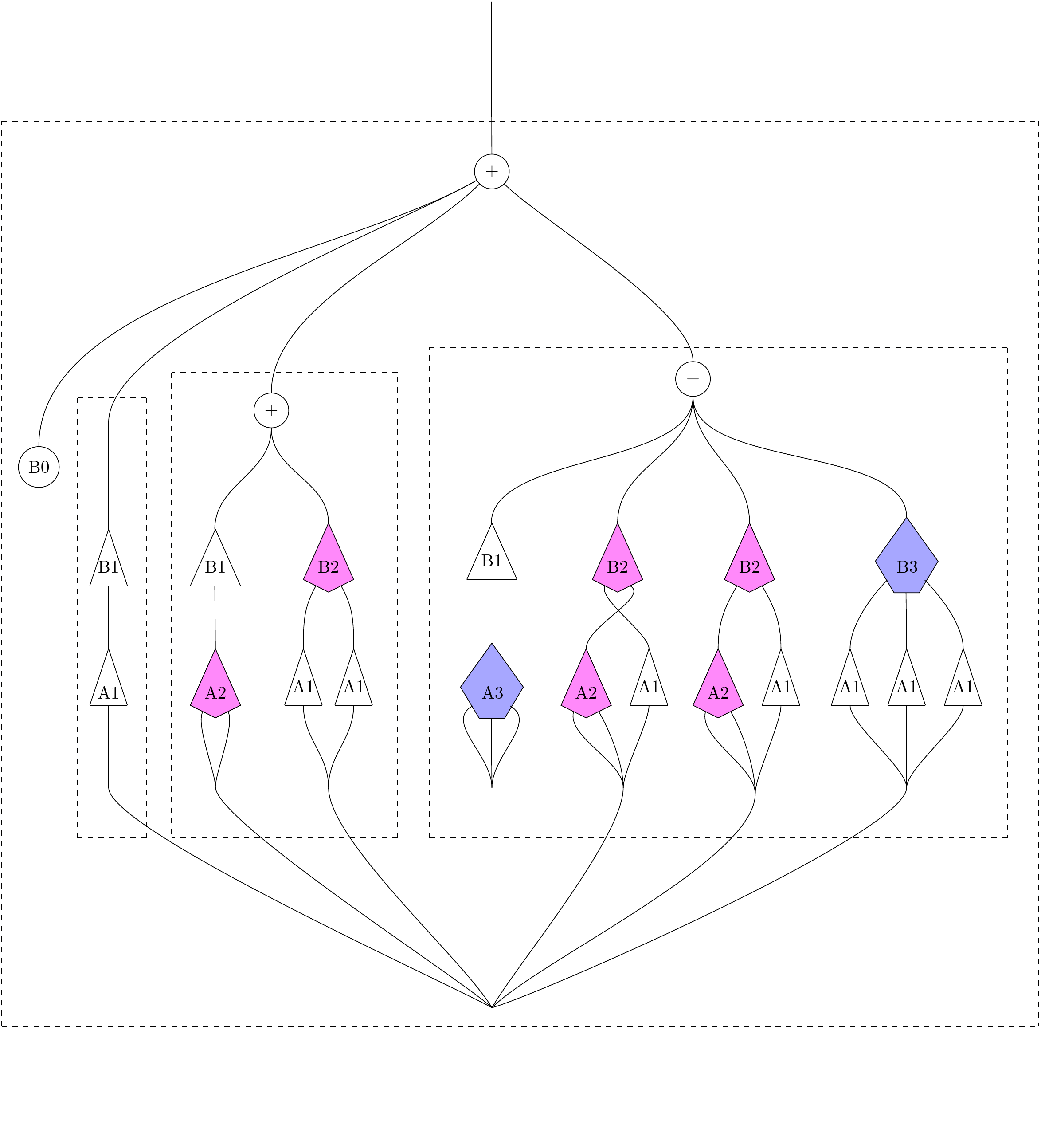
Figure 4.2: Binary series composition of Volterra series. The interior dashed boxes represent the composite homogeneous Volterra operators of the series composition $B\triangleleft A$.

4.3.1 Associativity of $\triangleleft$

Given three Volterra series, $C$, $B$, and $A$, there are two possible ways to use the binary composition rule to form the ternary composite of the series, such that the output of $A$ flows as the input to $B$ and the output of $B$ flows as the input to $C$; they are

$$C\triangleleft(B\triangleleft A)$$ (4.6)

and

$$(C\triangleleft B)\triangleleft A.$$ (4.7)

Equationally, these two types of ternary composition correspond to substituting eq. (4.5) into itself either for the operators of $A$ (i.e., at the first vertical level in Fig. 4.2) or for the operators of $B$ (at the second vertical level). The first of these forms of substitution is depicted in Fig. 4.3, and the second in Fig. 4.4.

Associativity implies that Figs. 4.3 and 4.4 must have the same number of boxes of each order (color), interconnected in the same pattern up to rearrangement; and yet, at first glance, they exhibit differences! For example, they have different numbers of order 1 (white, triangular) boxes. However, the following three assumptions and abuses of notation have been made in the design of these diagrams, which account for these variations. Firstly, constant multipliers appear wherever it is possible to permute the inputs to a colored box that is receiving its inputs from other homogeneous operators (i.e., excluding the first level boxes, whose inputs are inputs to the entire system). Secondly, certain wires in the second diagram split - a choice of visual presentation, which was made to avoid clutter. Thirdly, the zeroth order terms of the series $A$ and $B$ are assumed to be zero. This last simplifies the combinatorics, changing from weak compositions to merely compositions, and vastly reduces the number of non-trivial terms. Accounting for these permutations and conflations, one arrives, as a quick sanity check, at the following tally: that there are 90 white (unary) boxes; 17 magenta (dyadic) boxes; and 13 purple (triadic) boxes.

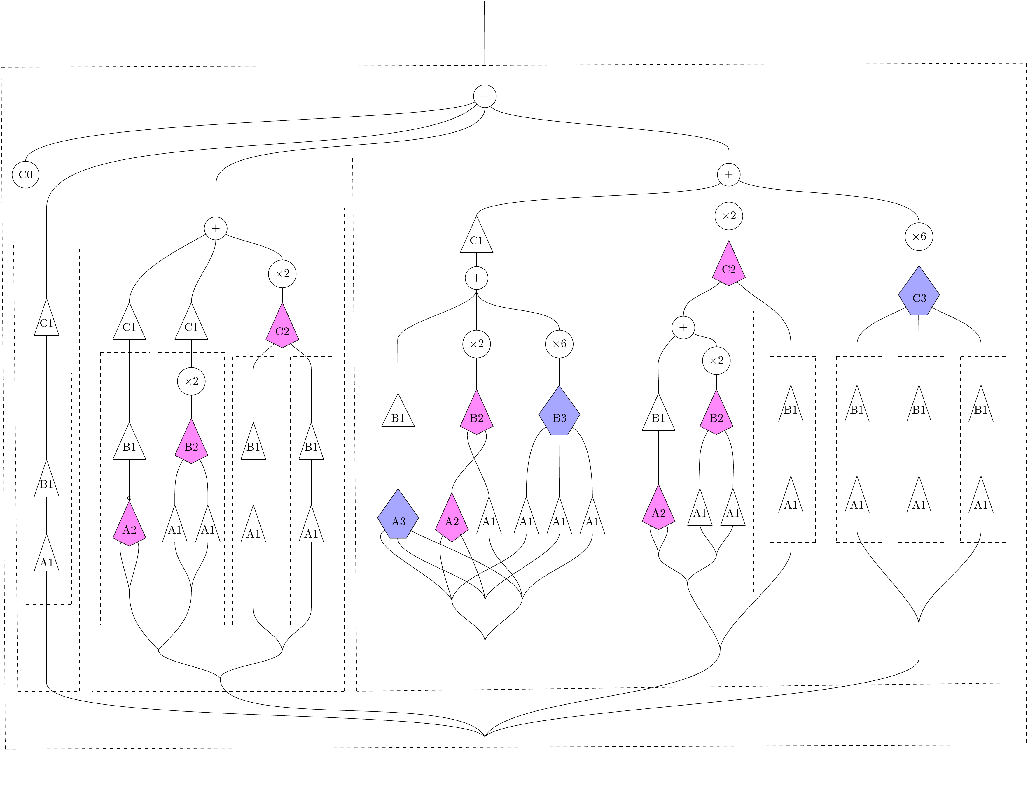
Figure 4.3: Ternary Series Composition, type 1: $C\triangleleft(B\triangleleft A)$. The interior-most dashed boxes represent composite homogeneous operators of $B\triangleleft A$, which are composed first from the operators of $B$ and $A$. The dashed boxes of the middle layer represent composite homogeneous operators of $C\triangleleft(B\triangleleft A)$, which are composed second from the operators of $C$ and $(B\triangleleft A)$.

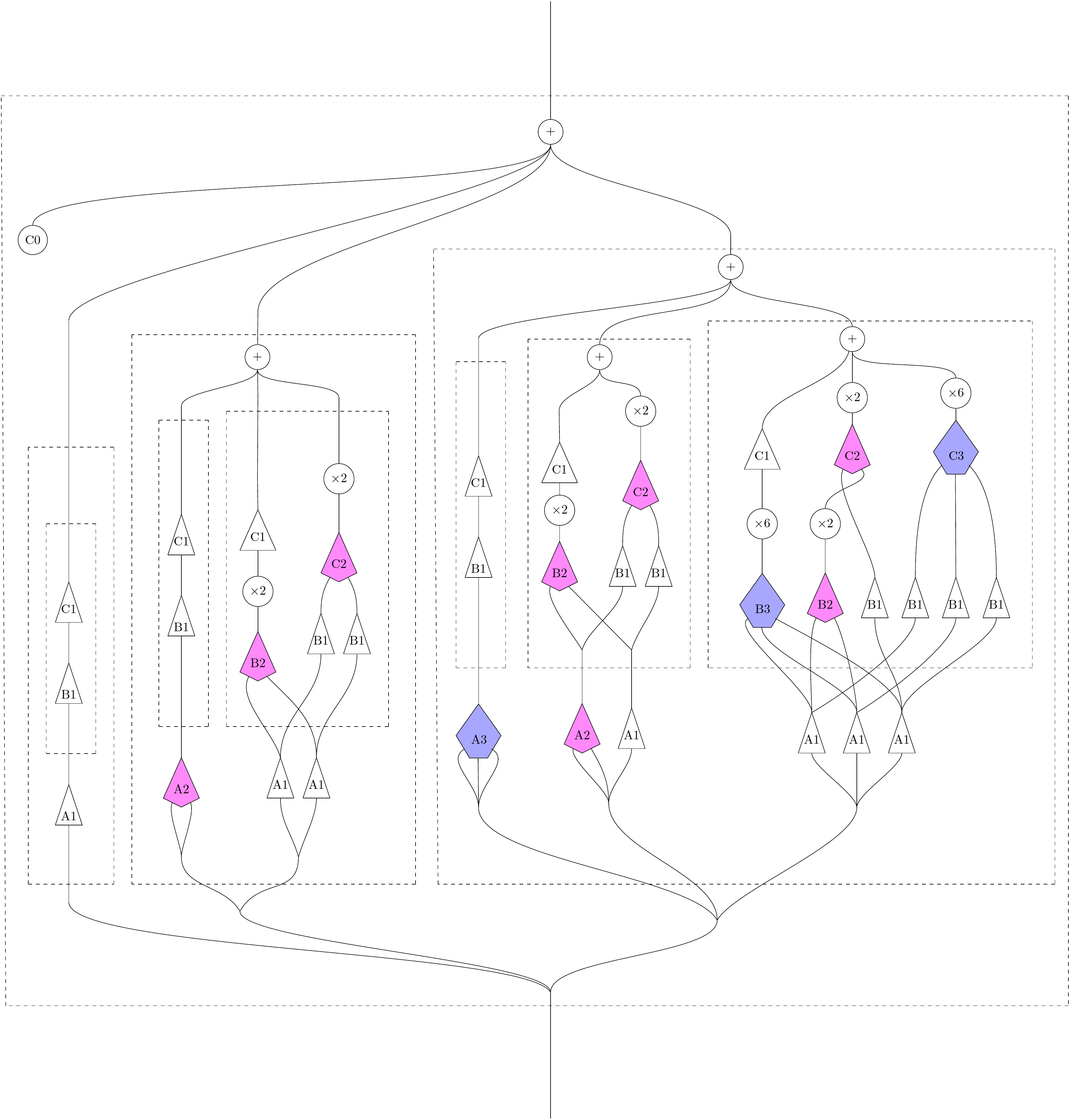
Figure 4.4: Ternary Series Composition, type 2: $(C\triangleleft B)\triangleleft A$. The interior-most dashed boxes represent the composite homogeneous operators of $C\triangleleft B$, which are composed first from the operators of $C$ and $B$. The dashed boxes of the middle layer represent the composite homogeneous operators of ($C\triangleleft B)\triangleleft A$, which are composed second from the operators of $(C\triangleleft B)$ and $A$.

In Appendix B, we prove that the two possible ways of composing three Volterra series using $\triangleleft$ are equivalent. That is, we prove

Theorem 1: The series composition, $\triangleleft$, of Volterra series is associative. I.e.,

$$(c\triangleleft(b\triangleleft a))_{j}\cong((c\triangleleft b)\triangleleft a)_{j}$$

for all $0\leq j\leq\infty$.

Proof: See Appendix B.

At a high level, the proof of Theorem 1 proceeds by constructing a bijection between:

1. The set of ways to compose the multivariate inputs, to each of the homogeneous operators of $C$, from the outputs of the homogeneous operators of the composite series $(B\triangleleft A)$;

2. The set of ways to compose the multivariate inputs, to each of the homogeneous operators of the composite series $(C\triangleleft B)$, from the outputs of the homogeneous operators of $A$.

One can think of these two possibilities for composing Volterra series in terms of stacking trees, as follows. Each $k^{\text{th}}-$order homogeneous operator is like a tree with $k$ branches. In each of the two cases, we are stacking trees (attaching the roots of some trees to the leaves of others) so as to form a composite tree of height (or depth) three that has $j-$many leaves. Theorem $1$ states that, for every order $j$, there is exactly the same number of such trees that can be formed through the first method above as there is through the second. The explicit bijection we construct is the content of equations (48) and (49), as well as of equation (50). It defines, essentially, the action of the associator of Volt with monoidal product the series composition product. The corresponding monoidal unit is the (linear) identity Volterra series that was described in Section $3.2.1.$, which has no effect when composed with any other series.

There are many other monoidal products on Volt, which we did not study. One, perhaps glaring ommission is the tensor product of Volterra series, which would describe a series whose output is the (multidimensional) tensor product of the outputs of the factors, and thus implicate the theory of multivariate Volterra series, as we saw with the series composition product. More generally, we should expect that any monoidal product on Poly, of which there are infinitely many, extends to one on Volt. Nonetheless, each of the three products covered in this chapter is fundamental, and together they allow us to describe interconnected nonlinear systems in which the outputs of subsystems are summed, multiplied, and/or fed into others (or themselves) as inputs.

Chapter 5 Time-frequency signal processing using Volterra series

The Fourier transform bridges between time and frequency, exchanging a temporal representation - based on elements that are of an instantaneous nature - for a spectral one - based on elements that are eternal, as they are periodic. Yet, we experience signals in the real world as having content that is at once temporal and frequential. For example, music and speech signals are perceived to have temporally-localized spectral data (the frequencies of a tone that rings out for a finite time, a melody that is sung). A more mathematical example is given by a chirp, whose Fourier transform informs us that, like an impulse, it contains energy at every frequency (sweeps the entire frequency spectrum); however, the information about when each frequency is present, and for how long is encoded by the phase information, which may appear difficult to interpret. In signal processing terms, the Fourier transform provides us with a picture of the signal that is stationary, but real signals have frequential content that is time-varying. They are evidently the products of nonstationary processes.

The field of time-frequency analysis arose to address the problem of the representation of signals jointly in time and frequency. Its core methods allow one to identify where, jointly in time and frequency, information in a signal is concentrated. Its modern formulation has its origins both in signal analysis and quantum mechanics [62], and is at the heart of audio signal processing. For a comprehensive account of (bilinear) time-frequency analysis, see [63, 64, 65] and for a classical treatment [66].

In this chapter, we introduce the bilinear time-frequency distributions along with their higher-order generalizations, and show how they can be embedded into Volt, thus enabling their future treatment using the results described in chapters 2, 3, and 4.

5.1 Time and frequency

Consider a (complex-valued) signal of the form

$$x(t)=A(t)e^{i\varphi(t)},$$ (5.1)

which is the product of a time-varying amplitude, $A(t)$, called the carrier, and a modulation term, $e^{i\varphi(t)},$ whose argument, $\varphi(t)$, is the signal phase. Such a signal is called analytic if its energy is distributed purely in the positive half of the frequency spectrum; this happens when $A(t)$ varies much more slowly than $\varphi(t)$, in which case the derivative of the phase can be interpreted as the instantaneous frequency of $x$ at time $t$ [67]:

$$f_{\text{inst}}(t)=\frac{1}{2\pi}\varphi^{{}^{\prime}}(t).$$ (5.2)

Though, in practice, signals are real-valued, if $s$ is a real signal then its complex analytic form can be obtained using the Hilbert transform, $H$, as

$$x(t)=s(t)+iH(s)(t)$$ (5.3)

where $H(x)(t)=\frac{1}{\pi}\text{p.v.}\int_{\tau\in\mathbb{R}}\frac{u(\tau)}{t-\tau}d\tau$ and where p.v. denotes the Cauchy principal value. Alternatively, $x(t)$ can be defined in the spectral domain, as

$$\hat{x}(f)=\begin{cases}2\cdot\hat{s}(f)&f>0\\ \hat{s}(f)&f=0\\ 0&f<0\end{cases}.$$

A natural way to represent the phase, $\varphi(t)$, is to let it be a polynomial function of time,

$$\varphi(t)=\sum_{p=0}^{P}a_{p}t^{p}.$$ (5.4)

Thus, for example, if $\varphi(t)=\beta t+c$, then the frequency is constant and the term $A(t)$ is modulated by a pure frequency and shifted by a constant phase term. If, instead, $\varphi(t)=\alpha t^{2}+\beta t+c$, then the signal includes a linear frequency modulation; and if $A(t)$ is a constant function, then the signal $x(t)$ is referred to as a (unit-amplitude, linearly frequency-modulated, or quadratic phase) chirp.

Energy distributions and representations

Of all the possible types of transformations, a representation is one that preserves the identity of any signal which it processes, but which may present it in an equivalent form. The Fourier transform is but one such example. A core property, important for physical interpretability, that such a transformation must satisfy is that it preserve the signal energy. Parseval’s theorem in Fourier analysis states that this property holds for the Fourier transform, i.e.:

$$E_{x}=\int_{t\in\mathbb{R}}|x(t)|^{2}dt=\int_{f\in\mathbb{R}}|X(f)|^{2}df$$ (5.5)

where $E_{x}$ is the energy of $x$. In the context of time-frequency distributions, which are bilinear, we search more generally for distributions of the form

$$\rho_{x}(t,f)=\frac{\partial^{2}E_{x}}{\partial t\partial f},$$

and so, for energies

$$E_{x}=\int_{t}\int_{f}\rho_{x}(t,f)dtdf$$ (5.6)

where $\rho_{x}$ is now the energy distribution of $x$. Such a distribution measures the energy density in both time and frequency, making it possible to locate where energy is present in the signal as it is represented in the time-frequency plane.

Distributions that preserve the signal energy may lose other forms of information. The spectrogram, for example, is a quadratic energy-preserving distribution that is obtained as the squared-magnitude of the STFT, and completely loses the spectral phase information. The Wigner-Ville distribution, which is in many respects the most important time-frequency distribution, in contrast preserves the signal energy and is invertible up to a constant phase factor, but is corrupted by interferences for multi-component signals. Atomic decompositions, which are linear representations, and amongst which the STFT is fundamental, are representations in the stronger sense of strict equality, yet they do not provide a measure of the local energy density of the signal jointly in time and frequency (but such densities can be obtained from them - as, e.g., the spectrogram is from the STFT).

We search, therefore, for representations akin to a musical score, capable of representing sequences of harmonies that are localized to particular intervals of time. However, just as a musical score provides a description of a piece of music in terms of information that is localized discretely, in units of duration and notes in a scale (or set of pitch classes), so, too, a time-frequency representation must navigate the fundamental tradeoff of time- and frequency resolution. This tradeoff can be stated in a number of ways, but a clear description is given in a signal processing context by the Balian-Low theorem. This theorem states that any family of elementary waveforms (called atoms) capable of representing the time-varying spectral structure of a signal, must have either infinite temporal or infinite spectral bandwidth. Formally, for any family of time-frequency atoms $h(t-nt_{0})e^{i2\pi mt\nu_{0}}$ generated from a finite-energy window function $h\in L^{2}(\mathbb{R})$, either

$$\int t^{2}|h(t)|^{2}dt=\infty\,\,\,\,\,\,\,\,\,\,\,\,\,\,\text{or \,\,\,\,\,\,\,\,\,\,\,\,\,\,$\int\nu^{2}|H(\nu)|^{2}d\nu=\infty$}.$$ (5.7)

An example of this principle is furnished by taking the family of atoms to the characteristic functions over finite interals, $h(t)=t_{0}^{-1/2}\boldsymbol{1}_{[0,t_{0}]}(t)$, whose Fourier transforms are the cardinal sine functions

$$\hat{h}(f)=t_{0}^{-1/2}e^{-\pi ift_{0}}\text{sinc}_{t_{0}}(t)$$

$$=t_{0}^{-1/2}e^{-\pi ift_{0}}\frac{\sin(\pi ft_{0})}{\pi ft_{0}};$$

these atoms provide a finite temporal bandwidth, but their bandwidth is analytic in the spectral domain. More generally, it is a fundamental fact in Fourier analysis that for any Fourier pair, the bandwidths in the two domains (here time and frequency) are inversely proportional (see [63] for a more in-depth account).

Given the fundamental obstruction that prevents the simultaneous attainment of optimal concentration in both time and frequency, much progress in time-frequency analysis has revolved around the developement of distributions that capture certain features of interest, but perhaps not others; for example, which are positive (allowing for interpretability as a probability density function), or optimally concentrated along the instantaneous frequency for some class of signals.

In section 5.1.1, we discuss the general form of time-frequency distributions, and focus on a central member of this class, the Wigner-Ville Distribution, which achieves optimal concentration along the instantaneous frequency of linearly frequency-modulated signals. We then describe, in section 5.1.2, how to represent these bilinear TFDs as Volterra series. We next show that the bilinear transformations cannot perfectly represent the time-varying spectral information of higher-order signals (i.e., signals whose instantaneous frequency varies nonlinearly, such as chirps of cubic or higher phase). This motivates the lift to so-called polynomial time-frequency distributions (PTFD), which we study in section 5.2.

5.1.1 Bilinear time-frequency distributions

The following is a review of the theory of bilinear time-frequency distributions. It largely follows the treatment in [63]; see there for more details.

In equation (5.6) we defined the energy of a signal in terms of a distribution $\rho(t,\nu)$, of two variables, one time and the other frequency. A general form of the distribution $\rho$ for a signal $x$ is

$$\rho_{x}(t,f)=\int\int K(u,u^{{}^{\prime}};t,f)x(u)x^{*}(u^{{}^{\prime}})du\,du^{{}^{\prime}}$$ (5.8)

which is parameterized by a kernel, $K:\mathbb{R}^{4}\rightarrow\mathbb{R}$, called the kernel of the analysis. Amongst all distributions of the form in (5.8), the time-frequency distributions as those that are covariant with respect to time-frequency shifts. A time-frequency shift is a linear transformation of the form

$$M_{\nu}T_{\tau}x(t)=x(t-\tau)e^{2\pi i\nu t}$$ (5.9)

where the operator $T$ shifts the signal by a constant in time, and the operator $M$ modulates (pointwise multiplies) it in the time domain by a constant frequency–which is equivalent to convolution by a delta function in the frequency domain (i.e., to a frequency shift). It is a fundamental fact that time and frequency shifts do not commute for all arguments $\tau$ and $\nu$

$$M_{\nu}T_{\tau}=e^{-2\pi i\tau\nu}T_{\tau}M_{\nu}.$$ (5.10)

However, they do commute when the product $\tau\nu$ is an integer. The time-frequency shifts generate the non-commutative group known as the Heisenberg-Weyl group.

Imposing that $\rho$ be covariant with respect to time-frequency shifts amounts to requiring that, for all signals $x$ and time-frequency shifts $T_{\tau}M_{\nu}$, the diagram in Fig. 5 commutes,

Figure 5.1: Covariance of time-frequency distributions with respect to time-frequency shifts.

which fact we denote by the right angle symbol in the upper left-hand corner. The action of the operator $\rho$ on the linear transformation of time-frequency shifting must equivalently be given by precomposition, $\rho(T_{\tau}M_{\nu})=\rho\circ T_{\tau}M_{\nu}$, which amounts in this case to shifting the kernel of the distribution. Thus, we have the following set of equivalences [63]

$$((\rho\circ T_{t^{{}^{\prime}}}M_{f^{{}^{\prime}}})(x))(t,f)=\rho_{x_{t^{{}^{\prime}}f^{{}^{\prime}}}}(t,f)=\rho(T_{t^{{}^{\prime}}}M_{f^{{}^{\prime}}})\rho_{x}(t,f)=\rho_{x}(t-t^{{}^{\prime}},f-f^{{}^{\prime}})$$

where

$$\rho_{x_{t^{{}^{\prime}}f^{{}^{\prime}}}}(t,f)=\int\int K(u+t^{{}^{\prime}},u^{{}^{\prime}}+t^{{}^{\prime}};t,f)e^{2\pi if^{{}^{\prime}}(u-u^{{}^{\prime}})}x(u)x^{*}(u^{{}^{\prime}})du\,du^{{}^{\prime}}$$

and

$$\rho_{x}(t-t^{{}^{\prime}},f-f^{{}^{\prime}})=\int\int K(u,u^{{}^{\prime}};t-t^{{}^{\prime}},f-f^{{}^{\prime}})x(u)x^{*}(u^{{}^{\prime}})du\,du^{{}^{\prime}}$$

and so, the representing kernel must satisfy

$$K(u,u^{{}^{\prime}};t-t^{{}^{\prime}},f-f^{{}^{\prime}})=K(u+t^{{}^{\prime}},u^{{}^{\prime}}+t^{{}^{\prime}};t,f)e^{2\pi if^{{}^{\prime}}(u-u^{{}^{\prime}})}.$$

Reorganizing, and performing a change of variables, one obtains

$$K(u,u^{{}^{\prime}};t,f)=K(u+t,u^{{}^{\prime}}+t;0,0)e^{2\pi if(u-u^{{}^{\prime}})}.$$ (5.11)

This says that time-frequency shifting the kernel function along both the time and frequency axes and then evaluating at the origin is equivalent to evaluating it at the point which is indexed by the two extents of the shift. Equation 5.8 for the time-frequency shift-covariant distributions can now be rewritten as

$$\rho_{x}(t,f)=\int\int K(s-t+\frac{\tau}{2},s-t-\frac{\tau}{2};0,0)x(s+\frac{\tau}{2})x^{*}(s-\frac{\tau}{2})e^{-i2\pi f\tau}d\tau\,ds$$

$$\rho_{x}(t,f)=\int\int\Pi(s-t,\xi-f)W_{x}(s,\xi)ds\,d\xi$$ (5.12)

where

$$W_{x}(s,f)=\int x(s+\frac{\tau}{2})x^{*}(s-\frac{\tau}{2})e^{-i2\pi f\tau}d\tau$$ (5.13)

is known as the Wigner-Ville Distribution (WVD) of the signal $x$, and

$$\Pi(t,f)=\int K(t+\frac{\tau}{2},t-\frac{\tau}{2};0,0)e^{2\pi if\tau}d\tau$$

is the inverse Fourier transform of the kernel.

A time-frequency distribution is thus a $2-$D convolution of the WVD of the signal with the inverse Fourier transform of the distribution kernel. The general form (5.12) can be rewritten more explicitly as

$$C_{x}(t,f;g)=\int\int\int e^{i2\pi\xi(s-t)}\phi(\xi,\tau)x(s+\frac{\tau}{2})x^{*}(s-\frac{\tau}{2})e^{-i2\pi f\tau}d\xi\,ds\,d\tau$$ (5.14)

where

$$\phi(\xi,\tau)=\int\int\Pi(t,f)e^{-i2\pi(f\tau+\xi t)}dt\,df$$

is an arbitrary parameter function. The form (5.14) is known as Cohen’s class of time-frequency distributions, and gives precisely the class of all bilinear distributions that are covariant with respect to time-frequency shifts. Further requiring conservation of energy

$$\int\int K(u-t,u^{{}^{\prime}}-t;0,0)e^{-i2\pi f(u-u^{{}^{\prime}})}dt\,df=\delta(u-u^{{}^{\prime}}),$$

implies that

$$\int\int\Pi(t,f)dt\,df=1,$$

and so $\phi(0,0)=1$.

In (5.14), the parameter function $\phi$ determines what, if any, additional features there are of the distribution kernel. If $\phi(\xi,\tau)=1,$ then we recover the WVD. If, instead, $\phi(\xi,\tau)=e^{2\pi i\xi\tau}$, then we have the Rihaczek distribution. The spectrogram, probably the most widely used TFD and the only one which is positive-definite (and so interpretable as a probability density function), is recovered by setting $\phi(\xi,\tau)=A_{h}^{*}(\xi,\tau)$, where $A_{h}(\xi,\tau)$ is the ambiguity function [63] of the short-time Fourier transform window $h$,

$$A_{h}(\xi,\tau)=\int h(s+\frac{\tau}{2})h^{*}(s-\frac{\tau}{2})e^{-i2\pi\xi s}ds.$$ (5.15)

We next turn to the WVD, which serves as a kind of prototype TFD from which all the others can be derived.

5.1.1.1 The role and properties of the Wigner-Ville Distribution

The WVD was originally developed in a quantum mechanical context by Wigner, who sought a joint position-momentum distribution to use in order to calculate deviations from equilibrium of a virial gas [62]. Although intended to function as a probability density function, it exhibits a feature which prevents its interpretation as such; namely, oscillatory interferences that are generated between the components of any multicomponent signal. Thus, the WVD is not, in general, everywhere positive. However, in other respects the WVD is ideal. In particular, it exhibits the property of being optimally concentrated around the instantaneous frequency for linearly FM signals; i.e., for any pair $(t,f)$, $W_{z}(t,f)=\delta(f-f_{\text{inst}}(t))$.

As shown, given a signal $z$, the WVD is the Fourier transform, with respect to $\tau$, of the time-shifted product of $z$ and its complex conjugate. Its mechanism of action can be understood as follows [71]. Let $z(t)$ be an analytic signal of unit magnitude, $z(t)=e^{i\varphi(t)}$. Then

$$W_{z}(t,f)=f\overset{F}{\leftrightarrow}\tau(K_{z}(t,\tau)),$$

where $f\overset{F}{\leftrightarrow}\tau$ denotes the partial Fourier transform which exchanges the $f,\tau$ variables, and $K_{z}(t,\tau)=z(t+\frac{\tau}{2})z^{*}(t-\frac{\tau}{2})=e^{i(\varphi(t+\frac{\tau}{2})-\varphi(t-\frac{\tau}{2}))}$. Recall that the instantaneous frequency (IF) of an analytic signal $e^{i\varphi(t)}$ is $f_{\text{inst}}(t)=\frac{1}{2\pi}\varphi^{{}^{\prime}}(t)$, which can be written

$$f_{\text{inst}}(t)=\frac{1}{2\pi}\lim_{\tau\rightarrow 0}\frac{\varphi(t+\tau/2)-\varphi(t-\tau/2)}{\tau},$$

where

$$2\pi\tau\hat{f}_{\text{inst}}(t,\tau)=\varphi(t+\tau/2)-\varphi(t-\tau/2)$$ (5.16)

is the (linear) central finite difference (CFD) approximation to the instantaneous frequency. We can then note that the values which the WVD takes at points $(t,f)$ in the time-frequency plane are computed using CFD estimates to the phase, scaled by the squared magnitude of the signal.

Because the CFD is a linear estimator, we expect the WVD to accurately measure the IF of signals whose frequency is varying linearly. Indeed, letting $\varphi(t)=\alpha t^{2}+\beta t$, we have that

$$W_{z}(t,f)=\int e^{i(\alpha(t+\tau/2)^{2}+\beta(t+\tau/2))}e^{-i(\alpha(t-\tau/2)^{2}+\beta(t-\tau/2))}e^{-i2\pi\tau f}d\tau$$

$$=\int e^{i(2\alpha t\tau+\beta\tau)}e^{-i2\pi\tau f}d\tau$$

$$=\int e^{-i2\pi\tau(f-\frac{1}{2\pi}(2\alpha t+\beta))}d\tau$$

$$=\delta(f-\frac{1}{2\pi}(2\alpha t+\beta)).$$ (5.17)

As mentioned, the WVD of a linear combination of signals is not the superposition of the component signals, oweing to its bilinear nature. For a signal $z=z_{1}+z_{2}$ which is the sum of two terms, $W_{z}=W_{11}+W_{12}+W_{21}+W_{22}$, where

$$W_{12}(t,f)=\int z_{1}^{*}(t-\frac{1}{2}\tau)z_{2}(t+\frac{1}{2}\tau)e^{-2\pi i\tau f}d\tau$$ (5.18)

is called the cross Wigner distribution. Though complex-valued, by Hermitian symmetry we have that $W_{12}=W_{21}^{*}$, and so

$$W_{z}=W_{11}+W_{22}+2\Re\{W_{12}\}.$$

More generally, for a signal $b$ which is a linear combination of signals, $b(t)=\stackrel{{\scriptstyle[}}{{n}}=1]{N}{\sum}b_{n}x_{n}(t)$, the WVD is of the form

$$W_{b}(t,f)=\stackrel{{\scriptstyle[}}{{n}}=1]{N}{\sum}|b_{n}|^{2}W_{x_{n}}(t,f)+2\stackrel{{\scriptstyle[}}{{n}}=1]{N-1}{\sum}\stackrel{{\scriptstyle[}}{{k}}=n+1]{N}{\sum}\Re\{b_{n}b_{k}^{*}W_{x_{n}x_{k}}(t,f)\}.$$ (5.19)

Much work has gone into reducing the interference terms of the WVD. For example, the parameter function $\phi$ in Cohen’s class may be used as an averaging kernel in order to smooth out the interferences that are oscillatory [63]. However, although the interference terms ruin the viability of interpretation of the WVD as a probability density function, they exhibit remarkable combinatorial and geometric structure. In particular, they are located exactly half-way along the line connecting the pairs of interacting components in the input signal, are oriented in the direction perpendicular to the line, and have a frequency depending on the distance between the components.

5.1.2 Volterra series representation of Cohen’s class

In [2], Powers and Nam showed that a class of double second-order Volterra series are equivalent to Cohen’s class of bilinear TFDs. Their result was motivated by the following observations:

1. Cohen’s class of time-frequency distributions has the form of a bilinear transformation wherein the input signal appears twice; and the $2^{\text{nd}}$-order (multivariate) Volterra series is a bilinear transformation of the same form.

2. The expression of Cohen’s class is parameterized in terms of a kernel function of two variables; and the $2^{\text{nd}}$-order Volterra series is also parameterized in terms of such a kernel.

3. All the members of Cohen’s class of bilinear distributions can be obtained from the WVD via a 2D convolution; and the $2^{\text{nd}}$-order Volterra series performs a 2D convolution.

We next recapitulate their result.

Second-order double Volterra series

Let $V$ be a Volterra series with two inputs, $x_{a}$ and $x_{b}$ , and all kernel functions zero except for $h_{2}$,

$$y(t)=H_{2}[x_{u},x_{v}]=\int\int h_{2}(u,v)\cdot x_{a}(t-u)x_{b}(t-v)du\,dv.$$ (5.20)

This was referred to in [2, 72] as a double, second-order VS, and further generalized by allowing the kernel function to be parameterized by a scalar variable $\theta$, as in

$$y(t,\theta)=\int\int h_{2,\theta}(u,v)\cdot x_{a}(t-u)x_{b}(t-v)du\,dv.$$ (5.21)

From the perspective of our framework, this could also be modeled as a family of Volterra series that are generated by a morphism which is parameterized by the variable $\theta$; i.e., $y(t,\theta)=\alpha_{\theta}(H_{2}(x_{u},x_{v}))(t)$, where $\alpha$ is a frequency-shift morphism, as described in section 3.2.3. (However, for the sake of consistency with respect to the notation of the articles we’re referring to, we preserve the original notation.)

By the time-shift properties of the Fourier transform, (5.21) can be rewritten

$$y(t,\theta)=\int\int\int\int h_{2,\theta}(u,v)\cdot e^{2\pi i(f_{1}+f_{2})t}\cdot e^{-2\pi i(f_{1}u+f_{2}v)}\cdot X_{a}(f_{1})X_{b}(f_{2})df_{1}df_{2}dudv$$

$$=\int\int H_{2,\theta}(f_{1},f_{2})\cdot e^{2\pi i(f_{1}+f_{2})t}\cdot X_{a}(f_{1})X_{b}(f_{2})df_{1}df_{2}$$ (5.22)

where $H_{2,\theta}$ is the $2-$D Fourier transform of the kernel function $h_{2,\theta}$. In the case where the two inputs $x_{a},x_{b}$ are given by

$$\begin{array}[]{c}x_{a}(t-u)=s^{*}(t-u)\\ \\ x_{b}(t-v)=s(t-v),\end{array}$$

then we have that $X_{a}(f_{1})=S^{*}(-f_{1})$ and $X_{b}(f_{2})=S(f_{2})$, so (5.22) becomes

$$y(t,\theta)=\int\int H_{2,\theta}(f_{1},f_{2})\cdot e^{2\pi i(f_{1}+f_{2})t}\cdot S^{*}(-f_{1})S(f_{2})df_{1}df_{2}.$$

Now, recall Cohen’s class of TFDs. Using once again the time-shift properties of the Fourier transform, (5.14) can be rewritten

$$C(t,f)=\int\int\int\delta(\xi+f_{1}+f_{2})\cdot e^{-2\pi i\xi t}\cdot\Phi_{2}(\xi,(f+\frac{1}{2}f_{1}-\frac{1}{2}f_{2}))d\xi\cdot S^{*}(-f_{1})S(f_{2})df_{1}df_{2}$$

$$=\int\int\Phi_{2}(-f_{1}-f_{2},(f+\frac{1}{2}f_{1}-\frac{1}{2}f_{2}))\cdot e^{2\pi i(f_{1}+f_{2})t}\cdot S^{*}(-f_{1})S(f_{2})df_{1}df_{2},$$

where $\Phi_{2}(\xi,\alpha)=\int\phi(\xi,\tau)\cdot e^{-2\pi i\alpha\tau}d\tau$, and $\phi$ is an arbitrary parameter function, as in (5.14). It can therefore be seen that Cohen’s class is precisely the class of double, $2^{\text{nd}}-$order Volterra series with kernel function of the form

$$\begin{array}[]{c}H_{2,f}(f_{1},f_{2})\\ \\ =\Phi_{2}(-f_{1}-f_{2},(f+\frac{1}{2}f_{1}-\frac{1}{2}f_{2}))\\ \\ =\int\phi(-f_{1}-f_{2},\tau)\cdot e^{-2\pi i(f+(1/2)f_{1}-(1/2)f_{2})\tau}d\tau.\end{array}$$ (5.23)

Note further that equation (5.23) is equivalent to

$$H_{2,f}(f_{1},f_{2})=\int\int\delta(\xi+f_{1}+f_{2})\phi(\xi,\tau)\cdot e^{-2\pi i(f+(1/2)f_{1}-(1/2)f_{2})\tau}d\tau d\xi.$$

Thus, $h_{2,f}(u,v)$ can be obtained via a $2-$D inverse Fourier transform, as

$$h_{2,f}(u,v)=\int\int\phi(\xi,\tau)\cdot e^{-2\pi if\tau}\cdot\int\int\delta(\xi+f_{1}+f_{2})\cdot e^{2\pi i[(u-\frac{1}{2}\tau)f_{1}+(v+\frac{1}{2}\tau)f_{2}]}df_{1}df_{2}d\tau d\xi$$

$$=\int\int\phi(\xi,\tau)\cdot e^{-2\pi if\tau}\cdot\delta(u-v-\tau)\cdot e^{-2\pi i(u-\frac{1}{2}\tau)\xi}d\tau d\xi$$

$$=e^{-2\pi if(u-v)}\cdot\int\phi(\xi,u-v)\cdot e^{\pi i(u+v)\xi}d\xi.$$ (5.24)

Cohen’s class can thus be described in Volterra series form as

$$C(t,f)=\int\int[h_{2,f}(u,v)]\cdot s^{*}(t-u)\cdot s(t-v)dudv$$

$$\int\int H_{2,f}(f_{1},f_{2})\cdot e^{2\pi i(f_{1}+f_{2})t}\cdot S^{*}(-f_{1})S(f_{2})df_{1}df_{2}$$

where $H_{2,f}(f_{1},f_{2})$ and $h_{2,f}(u,v)$ are as given in (5.23) and (5.24), respectively.

The WVD is a core member of Cohen’s class; it is obtained when $\phi(\xi,\tau)=1$, in which case the time- and frequency-domain kernels become

$$h_{2,f}(u,v)=e^{-2\pi if(u-v)}\delta(\frac{u+v}{2})=2e^{-4\pi ifu}\delta(u+v)$$

and

$$H_{2,f}(f_{1},f_{2})=\delta(f+\frac{1}{2}f_{1}-\frac{1}{2}f_{2}),$$

respectively. The Volterra series representation of the WVD can, in a sense, be read off from the standard definition by recognizing that the kernel function $h_{2,f}$ must comprise both the Fourier kernel and a delta functions that annihilates all but the symmetrically time-shifted copies of the input. The Volterra series representation of the WVD is thus

$$W(t,f)=\int\int 2e^{-2\pi if(u-v)}\delta(u+v)\cdot s^{*}(t-u)\cdot s(t-v)dudv$$ (5.25)

$$=\int\int\delta(f+\frac{1}{2}f_{1}-\frac{1}{2}f_{2})\cdot e^{2\pi i(f_{1}+f_{2})t}\cdot S^{*}(-f_{1})S(f_{2})df_{1}df_{2}.$$

5.2 Higher-order and polynomial time-frequency distributions

If the phase of a signal of the form (5.1) is not a polynomial of order two or lower, then the WVD is not optimally concentrated along the signal’s instantaneous frequency law; this is because the CFD estimate (5.16) of the phase is linear. For example, in the case of a cubic chirp signal, $s(t)=e^{i\varphi(t)}$, with $\varphi(t)=\gamma t^{3}/3+\beta t^{2}/2+\omega_{0}t$ and so $\varphi^{{}^{\prime}}(t)=\gamma t^{2}+\beta t+\omega_{o}$ , calculation of the WVD kernel results ([66], example 8.6) in

$$-\varphi(t-\frac{1}{2}\tau)+\varphi(t+\frac{1}{2}\tau)=\gamma\tau^{3}/12+(\gamma t^{2}+\beta t+\omega_{0})\tau$$

$$=\gamma\tau^{3}/12+\varphi^{{}^{\prime}}(t)\tau$$

from which it follows that

$$\begin{array}[]{c}W_{z}(t,f)=\frac{1}{2\pi}\int e^{i\gamma\tau^{3}/12+i(\varphi^{{}^{\prime}}(t)-\omega)\tau}d\tau\\ \\ =\frac{2}{2\pi}(\frac{4}{\gamma})^{1/3}\int\cos[\gamma\tau^{3}/12+(\varphi^{{}^{\prime}}(t)-\omega)\tau]d\tau\\ \\ =(\frac{4}{\gamma})^{1/3}\text{Ai}((\frac{4}{\gamma})^{1/3}[\varphi^{{}^{\prime}}(t)-\omega])\end{array}$$

where $\text{Ai}(x)$ is the Airy function $\text{Ai}(x)=\frac{1}{\pi}\int_{0}^{\infty}\cos(u^{3}/3+xu)du$. What is more, no bilinear TFD can overcome this limitation, since they are all obtained from the WVD by the operation of convolution. This motivates the search for higher-order time-frequency representations, capable of modeling nonstationary signals of a more strongly nonlinear nature.

5.2.1 The Polynomial Wigner-Ville Distribution

In [71, 73, 74, 75, 76], higher-order analogues of the WVD were described, generalizing the WVD to the ‘time-multifrequency’ (or ‘multi-time, multi-frequency’) setting. A core member of these transforms is the Higher-Order Wigner-Ville Distribution (HOWVD), defined by

$$W_{x}^{(k)}(t,\boldsymbol{f})=\int_{\boldsymbol{\tau}\in\mathbb{R}^{k-1}}x^{*}(t-\alpha_{k})\prod_{r=1}^{k-1}P_{r+1}\{x(t+\tau_{r}-\alpha_{k})\}e^{-i2\pi\boldsymbol{f}^{T}\boldsymbol{\tau}}d\boldsymbol{\tau}$$ (5.26)

where $\boldsymbol{f}\in\mathbb{R}^{k-1}$, $P_{r}(x)=\begin{cases}x^{*}&r\text{ odd}\\ x&\text{else}\end{cases}$, $\boldsymbol{\tau}=\{\tau_{1},\dots,\tau_{k-1}\}$, and $\alpha_{k}=\frac{1}{k}\sum_{r=1}^{k-1}\tau_{r}$. It is a straightforward extension of the WVD to higher dimensions.

It was shown in [76] that any HOWVD uniquely determines a two-dimensional distribution, called the Polynomial Wigner-Ville Distribution (PWVD), which is of the form

$$W_{x}^{(k)}(t,f)=\int_{\tau}x^{*}(t+\lambda_{1}\tau)\prod_{r=1}^{k-1}P_{r+1}\{x(t+\lambda_{r+1}\tau)\}e^{-i2\pi f\tau}d\tau$$ (5.27)

where $k$ is even and the coefficients $\lambda_{r},$ $r=1,\dots,k$ satisfy a set of nonlinear equations. It is obtained from the HOWVD as a projection from multifrequency to one-dimensional frequency space, with projection axis

$$f=\frac{f_{r}}{\lambda_{r+1}+\sum_{l=1}^{k-1}\lambda_{l+1}},\,\,(r=1,\dots,k-1)$$

and corresponding slice axis

$$\tau_{r}=(\lambda_{r+1}+\sum_{l=1}^{k-1}\lambda_{l+1})\tau\,\,(r=1,\dots,k-1).$$ (5.28)

The PWVD was also used to define a ‘higher Cohen’s class’ of TFDs [73].

Like the WVD, the PWVD is a function of time and frequency, but unlike the WVD it exhibits optimal concentration along the IF for signals whose phase is an arbitrary polynomial of order less than or equal to that of the distribution. That is, for a constant-amplitude analytic signal of the form $z(t)=Ae^{i\varphi(t)}$, where $\varphi(t)$ is a polynomial of order $P$, $\varphi(t)=\sum_{r=0}^{P}a_{r}t^{r}$, then for a certain selection of the coefficients $\lambda_{r}$, we have that

$$W_{z}^{(k)}(t,f)=A^{k}\delta(f-\frac{1}{2\pi}\sum_{m=1}^{P}ma_{m}t^{m-1})$$ (5.29)

where $A$ is the constant amplitude of the analytic signal. Note that eq. (5.29) implies that

$$\arg\{\prod_{r=1}^{k/2}z(t+\lambda_{r}\tau)z^{*}(t+\lambda_{-r}\tau)\}=\tau\sum_{m=1}^{p}ma_{m}t^{m-1}.$$ (5.30)

Substituting $Ae^{i\varphi(t)}$ for $z$ in the left-hand side of (5.30), and letting $t=0$, we arrive at

$$\arg\{\prod_{r=1}^{k/2}e^{i\varphi(t+\lambda_{r}\tau)-i\varphi(t+\lambda_{-r}\tau)}\}=\arg\{\prod_{r=1}^{k/2}e^{i(\sum_{m=0}^{P}a_{m}(\lambda_{l}\tau)^{m}-\sum_{m=0}^{P}a_{m}(\lambda_{-l}\tau)^{m})}\},$$

and so

$$\sum_{m=0}^{p}\sum_{r=1}^{k/2}a_{m}[\lambda_{r}^{m}+(-1)\lambda_{-r}^{m}]=0\cdot a_{0}+1\cdot a_{1}+0\cdot a_{2}+...+0\cdot a_{p}.$$ (5.31)

Equation (5.31) implies that the property of concentration along the IF of a polynomial phase signal requires that the coefficients $\lambda_{r}$ satisfy a nonlinear set of equations, namely:

$$\sum_{r=1}^{k/2}(\lambda_{r}-\lambda_{-r})=1$$

and

$$\sum_{r=1}^{k/2}(\lambda_{r}^{m}-\lambda_{-r}^{m})=0,\,\,\,m=2,...,p;$$

or, equivalently,

$$\begin{array}[]{c}\lambda_{r}=-\lambda_{r-1}\,\,\,(r=1,...,k/2)\\ \\ \stackrel{{\scriptstyle[}}{{r}}=1]{k/2}{\sum}\lambda_{r}=1/2\\ \\ \stackrel{{\scriptstyle[}}{{r}}=1]{k/2}{\sum}\lambda_{r}^{m}=0\end{array}$$ (5.32)

for $m\text{ odd};m=3,...,p$.

The equations (5.32) have no exact, real solutions for $p=3$ or $p=4$ for $k\leq 4$, nor for $p=6,8,...,$ by the Abel-Ruffini theorem. For $p=3$ or $p=4$ with $k=6$, there is an infinite family of solutions given by

$$\begin{array}[]{c}\lambda_{1}=\frac{1}{4}-\frac{\lambda_{3}}{2}\pm\frac{\sqrt{3}\sqrt{24\lambda_{3}^{3}+12\lambda_{3}^{2}-6\lambda_{3}+1}}{12\sqrt{2\lambda_{3}-1}}\\ \\ \lambda_{2}=\frac{1}{4}-\frac{\lambda_{3}}{2}\mp\frac{\sqrt{3}\sqrt{24\lambda_{3}^{3}+12\lambda_{3}^{2}-6\lambda_{3}+1}}{12\sqrt{2\lambda_{3}-1}},\end{array}$$ (5.33)

where, in order that $\lambda_{1}$ and $\lambda_{2}$ exist and are real, we must have that $\lambda_{3}\geq\frac{1}{2}$ [71].

Proof of formula (5.33) [Depalle]:

Denote by $s=\lambda_{1}+\lambda_{2}=\frac{1}{2}-\lambda_{3}$ and $p=\lambda_{1}\lambda_{2}=\frac{1}{3}(\frac{s^{3}+\lambda_{3}^{3}}{s})$ the product and sum of the roots $\lambda_{1}$ and $\lambda_{2}$. Then they are solutions to $x^{2}-sx+p=0$, and so are of the form

$$s^{2}-4p$$

$$=s^{2}-\frac{4}{3}(\frac{s^{3}+\lambda_{3}^{3}}{s})=-\frac{1}{3}(\frac{s^{3}+4\lambda_{3}^{3}}{s})$$

$$=-\frac{1}{3}\left(\frac{(\frac{1}{2}-\lambda_{3})^{3}+4\lambda_{3}^{3}}{\frac{1}{2}-\lambda_{3}}\right)=-\frac{1}{3}\left(\frac{(1-2\lambda_{3})^{3}+32\lambda_{3}^{3}}{4(1-2\lambda_{3})}\right)$$

$$=-\frac{1}{12}\left(\frac{1-6\lambda_{3}+12\lambda_{3}^{2}-8\lambda_{3}^{3}+32\lambda_{3}^{3}}{1-2\lambda_{3}}\right)=\frac{24\lambda_{3}^{3}+12\lambda_{3}^{2}-6\lambda_{3}+1}{12(2\lambda_{3}-1)}$$

from which it follows that

$$\lambda_{1,2}=\frac{1}{4}-\frac{\lambda_{3}}{2}\pm\sqrt{3}\cdot\frac{\sqrt{24\lambda_{3}^{3}+12\lambda_{3}^{2}-6\lambda_{3}+1}}{12\sqrt{(2\lambda_{3}-1)}}.$$

Some properties of the PWVD were reported in [71]; for example, the PWVD is covariant with respect to time-frequency shifts, and distributes over modulation. Experiments were also performed demonstrating the benefit brought by the PWVD when compared to bilinear distributions such as the WVD; for example, it was shown in [71], example 3.6.2 that for a quadratic chirp signal which is modulated by white Gaussian noise, the $4^{\text{th}}-$order PWVD, written

$$W_{z}^{(4)}(t,f)=\int[x(t+\tau/4)]^{2}[x(t-\tau/4)]^{2}e^{-2\pi i\tau f}d\tau,$$

is clearly concentrated along the linear time-varying frequency component, whereas the WVD of the same signal is unreadable.

5.2.2 Volterra series representation of the Polynomial WVD

In order to render the PWVD in Volterra series form, we need to internalize the conditions from (5.32) as components of the Volterra kernel function, $v_{k}^{\text{PWVD}}$. We will use the following symmetric notation for the PWVD

$$W_{z}^{(k)}(t,f)=\int_{\tau\in\mathbb{R}}e^{-2\pi if\tau}\prod_{l=1}^{k/2}z(t+\lambda_{l}\tau)\cdot z^{*}(t+\lambda_{-l}\tau)d\tau$$ (5.34)

where the coefficients $\lambda_{l}$, $l=(1,\dots,\frac{k}{2})$, must satisfy the set of equations (5.32). Notice that this form is nearly identical to a Volterra series with Fourier kernel function, but for the coefficients $\lambda_{l}$.

Recall from equation 5.28 that the variable of integration, $\tau$, is the unique slice of a multidimensional parameter $\boldsymbol{\tau}_{k}\in\mathbb{R}^{k}$, and is related to the coefficients $\lambda_{l}$. Just as the Volterra series form of the WVD involves a component that is a delta distribution, so do we impose that $\tau$ take on only those values that satisfy the constraint in (5.32); we do this by incorporating, into the Volterra kernel function, terms that are composed of delta distributions which annihilate the signal energy outside the solution set for the variable of integration, $\boldsymbol{\tau}_{k}$.

Let $v_{k}^{{}^{\prime}}(\boldsymbol{\tau}_{k})=ke^{-2\pi if(\sum_{l=-k/2}^{k/2}\tau_{l})}$ denote the multidimensional Fourier kernel function of a Volterra series, which we would like to exhibit the properties of the PWVD, and let $v_{k}^{\text{PWVD}}(\boldsymbol{\tau}_{k})$ denote the true PWVD kernel function. Then the first condition of (5.32) on the coefficients $\lambda_{l}$ translates into a constraint on the kernel function, as

$$\lambda_{l}=-\lambda_{l-1}\,\,\,(l=1,...,k/2)\implies v_{k}^{\text{PWVD}}(\boldsymbol{\tau}_{k})=v_{k}^{{}^{\prime}}(\tau_{k})\prod_{l=1}^{k/2}\delta(\tau_{l}+\tau_{-l});$$

the second, as

$$\stackrel{{\scriptstyle[}}{{l}}=1]{k/2}{\sum}\lambda_{l}=1/2\implies v_{k}^{\text{PWVD}}(\boldsymbol{\tau}_{k})=v_{k}^{{}^{\prime}}(\boldsymbol{\tau}_{k})\delta(\left[\sum_{l=1}^{k/2}\tau_{l}\right]-1/2);$$

and the third, as

$$\stackrel{{\scriptstyle[}}{{l}}=-k/2]{k/2}{\sum}\lambda_{l}^{m}=0\implies v_{k}^{\text{PWVD}}(\boldsymbol{\tau}_{k})=v_{k}^{{}^{\prime}}(\boldsymbol{\tau}_{k})\delta(\sum_{l=-k/2}^{k/2}\tau_{l}^{m}).$$

Putting these terms together results in the kernel function

$$v_{k}^{\text{PWVD}}(\boldsymbol{\tau}_{k})=\left[\prod_{l_{1}=1}^{k/2}\delta(\tau_{l_{1}}+\tau_{-l_{1}})\right]\cdot\delta\left(\sum_{l_{2}=-k/2}^{k/2}\tau_{l_{2}}^{m}\right)\cdot\delta\left(\left[\sum_{l_{3}=1}^{k/2}\tau_{l_{3}}\right]-1/2\right)\cdot ke^{-2\pi if\left(\sum_{l=-k/2}^{k/2}\tau_{l}\right)}.$$ (5.35)

Thus, as a $k^{\text{th}}-$order Volterra series, (5.34) is of the form

$$V_{z}^{\text{PWVD}}(t,f)=\int_{\boldsymbol{\tau}_{k}\in\mathbb{R}^{k}}v_{k}^{\text{PWVD}}(\boldsymbol{\tau}_{k})\prod_{l=1}^{k/2}z_{l}(t+\tau_{l})\cdot z^{*}(t+\tau_{-l})d\tau_{l}d\tau_{-l},$$ (5.36)

where $v_{k}^{\text{PWVD}}(\boldsymbol{\tau}_{k})$ is as in (5.35).

Following [73], equation (5.36) can also be used to define a class of Volterra series generalizing Cohen’s class to higher dimensions:

$$C_{z}^{\text{(k)}}(t,f)=\int_{\boldsymbol{\Omega}_{k}\in\mathbb{R}^{k}}e^{-2\pi it\sum\Omega_{k}}\cdot\hat{v}_{k}^{\text{PWVD}}(\boldsymbol{\Omega}_{k})\cdot c_{k}(\boldsymbol{\Omega}_{k})\prod_{m=1}^{k/2}\hat{z}_{m}(\omega_{m})\cdot\hat{z^{*}}(\omega_{-m})d\omega_{m}d\omega_{-m}$$

where $c_{k}:\mathbb{R}^{k}\rightarrow\mathbb{R}$ is the smoothing parameter function, and $\boldsymbol{\Omega}_{k}=[\omega_{-k/2},\dots,\omega_{-1},\omega_{1},\dots,\omega_{k/2}]$ is the $k-$dimensional vector of frequency variables.

Composing time-frequency representations

Time-frequency representations are unique amongst nonlinear systems in that they fundamentally preserve the signal information, rather than change it. Consequently, these systems stand in a different relation to the possible aims of any audio signal processing framework than those that alter the identity of the audio signals which they process. In particular, composing time-frequency representations using the methods of Chapter 4 - for example, in series - will result in systems that simply reexpress, potentially in new ways, the essences of signals that are input to them.

The power of time-frequency representations lies, rather, in their ability to provide different views onto the information contained in a signal. The ability of the PWVD, for example, to clearly reveal the time-frequency content of a nonlinearly frequency-modulated signal means that areas in the time-frequency plane where energy is present in the signal can be identified and targeted in a subsequent transformation. The benefit brought by incorporating time-frequency representations into a general nonlinear signal processing framework therefore lies in enabling the conjoined usage of representational and non-representational systems. Complex nonlinear audio signal processing chains might be constructed consisting of higher-order time-frequency representations that are composed with complex filtering processes. In this light, morphisms of time-frequency distributions might serve as an elegant mechanism for the controlled nonlinear editing of audio that is represented across different dimensions of time-frequency space.

Conclusion and prospects

In this work, we have layed the foundation of a compositional approach to nonlinear audio signal processing that is based on the Volterra series, a universal model of nonlinear dynamics. We have done so by categorifying the VS. Specifically, we showed what it would mean for the Volterra series to be a functor on the category $S^{\prime}(\mathbb{R})$ whose objects are signals or spectra, and whose morphisms are multipliers or convolutors; and we interpreted the condition of functoriality in terms of the effect that processing a signal linearly would have on a subsequent nonlinear processing. This allowed us to obtain, in the cases of certain types of linear transformations, representations of the nonlinear output in terms of a series sum of linear transformations applied to the homogeneous outputs of the associated Volterra series.

We then defined morphisms of Volterra series using a lens map construction. This lead us directly to a definition of the category Volt, a kind of universe of nonlinear systems. We studied three elementary monoidal products on Volt: sum, product, and series composition; and we proved that the third of these is associative, thereby exhibiting Volt as a monoidal category. Thus, we set on firm theoretical ground a compositional approach to the representation of complex nonlinear systems and their transformations - an approach that is sensitive to weaker notions than strict equality, such as equivalence up to reassociation of systems composed in series.

We turned to the theory of bilinear time-frequency distributions – which are essential to audio – and their higher-order counterparts, in particular to the polynomial TFDs. We reviewed an equivalence between Cohen’s class of TFDs and a subclass of second-order double Volterra series, and showed how it extends to one between the polynomial TFDs and a class of higher-order VS, thus providing a new bridge whereby higher TFDs may be treated using Volterra series methods.

Future work

The theory we have described could be extended or generalized in a number of directions. For example, we did not discuss the analysis – or decomposition – and identification of nonlinear systems via probing techniques [7], although this is of critical practical importance and a major subject in the VS literature. Such techniques can also be used to solve for the parameters of entire classes of nonlinear systems algebraically, as shown in [77]. Related to identification techniques are order separation methods, which are used to preprocess Volterra series models and speed up subsequent probing-based procedures. An interesting example of order separation is given by the phase-based technique of Bouvier et al. [78]. Nonlinear system identification methods stand, moreover, to benefit greatly from compositionality, since if the components in a factorization can be identified separately then the results can be combined, resulting in multiplicative gains. In a similar vein to identification, it would be useful to study regularization techniques, such as those presented in [79, 80], in order to reduce the sensitivity of system identification techniques to edge-cases or anomolous patterns of behavior.

We only gave, moreover, a tiny sampling of the various interesting and even fundamental transforms that are contained in Volt, any number of which might serve in a useful and structural role, and many of which already have known applications. For example, in higher-dimensional signal processing, the Riesz transform plays a role analogous to that of the Hilbert transform in classical signal processing. It has been used, e.g., in demodulation of speech signals [81] as well as fringe patterns in optics [82]. It could be fruitful to study the Volterra series representations of known transforms, and integrate them into new nonlinear audio processing chains within our framework.

Additionally, in our explorations we have only scratched the surface of the abstract categorical structure of Volt. A programme for elucidating this could follow, as a roadmap, the development of the theory of polynomial functors as described in [55], since Volterra series appear to be to signals what polynomial functors are to sets. However, we did not prove, but only conjectured, the functoriality of the Volterra series - a major supposed link to that work - so providing a proof or disproof of that conjecture is the immediate next step. More specifically, we suspect, and would like to show, that in analogy to polynomial functors, the Volterra series is a sum of representable functors - and that these are the homogeneous Volterra operators.

Although we have treated only Volterra series which process inputs and produce outputs that are elements of $S^{\prime}(\mathbb{R})$, and whose kernels are elements of $S^{\prime}(\mathbb{R}^{n})$, other domains than $\mathbb{R}$ can be considered for use in constructing the signal space. In particular, one can define graph Volterra series, which process signals that are elements of a signal space, $S^{\prime}(G)$, that is defined over a graph $G$. Convolution and spectral analysis are then carried out over powers of the underlying graph via spectral decompositions of a graph shift operator, in particular the graph Laplacian. Such decompositions can be obtained via elementary products of the matrix representation of the operator: for example, given a graph $G$, the Laplacian matrix of their Cartesian product is of the form $L(G\times G)=L(G)\otimes I_{n}+I_{m}\otimes L(G)$, where $\otimes$ is the Kronecker product; an associated eigenbasis is obtained via $L(G\times G)(X_{i}\otimes Y_{j})=(\lambda_{i}+\mu_{j})(X_{i}\otimes Y_{j})$, where $X_{i},Y_{j}$ are eigenvectors and $\lambda_{i},\mu_{j}$ are associated eigenvalues. We expect that there would be many interesting uses for other graph products, as well - 256 of which are reported in [83] that are generated from the adjacency, non-adjacency, and equality relations, alone.

Moreover, just as the field of time-frequency bridges between time and frequency for signals indexed over $\mathbb{R}$, the recent field of ‘vertex-frequency graph signal processing’ plays an analogous role for signals over graph, bridging between the graph signal and graph spectral domains [32]. Furthermore, the theory of graphons [36, 35, 34, 33] in principle allows for discrete methods to be obtained from continuous ones via sampling operations, and so for a corresponding continuous theory of graph-based Volterra series to be developed.

More generally, it should be possible to lift much if not all of the formalism developed in this work to the setting of nonlinear signal processing over simplicial complexes or other higher models of space, wherein associated continuous theories would be obtained in the limit of refinement. The inputs, outputs, and kernel functions of Volterra series could even be formally defined over structured spaces such as manifolds - e.g., over the $d-$dimensional torus, $\mathbb{T}^{d}$ - with morphisms of Volterra series being suitably adapted in like kind. It would be interesting to explore the structure and uses of morphisms between Volterra series defined over such spaces, including potential connections with the circle maps described in [51].

Appendix A: Construction of the category $S^{\prime}(\mathbb{R})$

In this appendix, we construct the base category, $S^{\prime}(\mathbb{R})$. Its collection of objects is the union of the set of signals and the set of spectra, and its morphisms are certain linear transformations. It is this category over which, we conjecture, Volt exists as a functor category. Since the ability to work in the spectral domain is crucial to the use and formalization of Volterra series, we are compelled to define signals and their spectra as elements of the Schwartz space and its dual - i.e., to functions that are rapidly decreasing at infinity and to distributions that are slowly growing at infinity, respectively - since it is precisely for these objects that the Fourier integral is well-defined. We provide in this appendix a review, largely drawn from [84], of the relevant notions from functional and harmonic analysis, but our recapitulation is quite sparse; see [85], [86], [87] for a fuller treatment.

Linear Operators

Consider a signal $u:\mathbb{R}\rightarrow\mathbb{C}$. A system is linear iff it obeys the superposition and proportionality constraints:

$$\begin{array}[]{c}L(u+u^{\prime})=L(u)+L(u^{\prime})\\ \\ L(c\cdot u)=c\cdot L(u)\end{array}$$

for any other $u^{\prime}:\mathbb{R}\rightarrow\mathbb{C}$ and $c\in\mathbb{C}$. Linear systems come in two important classes. To introduce them, we need the following two elementary operators.

The modulation of $u$ by a frequency $\xi\in\mathbb{\hat{R}}$ , where $\hat{\mathbb{R}}$ denotes the unitary dual of $\mathbb{R}$, i.e. the space of functions $e_{\xi}(x)=e^{2\pi ix\cdot\xi}$, by

$$M_{\xi}u(x)=e^{2\pi ix\cdot\xi}u(x).$$

The translation of $u$ by $\tau\in\mathbb{R}$ is given by

$$T_{\tau}u(x)=u(x-\tau).$$

Any linear operator, $L$, that commutes with translations is referred to as a linear, time-invariant (LTI) system. It satisfies the property

$$y(t+\tau)=(L\circ T_{\tau})s(t)=(T_{\tau}\circ L)s(t)$$

for all constants $\tau\in\mathbb{R}$, where $y(t+\tau)$ is the system output at time $t+\tau$. Dually, we might call any linear operator commuting with $M$ a linear frequency-invariant (LFI) system. An important characterization of LTI systems is that they do not increase the frequency-domain support of the signals which they process; likewise, LFI systems do not increase the temporal support of signals.

Recall the integral definition, given in (4), of the Fourier transform, $F$. Modulations and translations satisfy the following set of equations

$$\begin{array}[]{c}F\circ M_{\xi}=T_{\xi}\circ F\\ \\ F\circ T_{\tau}=M_{-\tau}\circ F\end{array}$$

Thus, we see that translations and modulations do not, exactly, commute; rather, we have that

$$T_{\tau}M_{\xi}=e^{-2\pi i\tau\cdot\xi}M_{\xi}T_{\tau}$$

(and, so, they do commute when the product $\tau\cdot\xi$ is an integer).

Another linear operator that has an important relationship with the Fourier transform is complex conjugation, $z\mapsto\bar{z}$. Its interaction with $F$ is given by

$$F(\iota(\bar{u}))=\overline{Fu}$$

where $\iota u(t)=u(-t)$ denotes the reflection of the signal $u$ about zero. We will use this when defining the operation of convolution by a tempered distribution. First, we recall the operation of convolution of functions: given two absolutely integrable functions, $u,v\in\mathbb{R}\rightarrow\mathbb{C}$, their convolution is another function, $u\ast v:\mathbb{R}\rightarrow\mathbb{C}$, defined by the formula

$$(u\ast v)(t)=\int u(t-\tau)v(\tau)d\tau.$$

Convolution is associative and commutative. A central result in Fourier analysis and signal processing is the convolution theorem, which states that the Fourier transform interchanges convolution and pointwise-multiplication

$$\widehat{u\ast v}(\xi)=\hat{u}(\xi)\hat{v}(\xi).$$

The spaces $\mathscr{S}(\mathbb{R})$ and $\mathscr{S}^{{}^{\prime}}(\mathbb{R})$

We now turn to the Schwartz space of rapidly decreasing functions and its dual, the space of tempered distributions. Denote by $\mathscr{C}^{\infty}(\mathbb{R})$ the space of infinitely differentiable, or smooth, functions. For $\alpha,m\in N_{0}$, and $K$ a compact subset of $\mathbb{R}$, $\mathscr{C}^{\infty}(\mathbb{R})$ becomes a topological vector space when equipped with the family of seminorms $\varphi\mapsto|\varphi|_{m,K}$, where

$$|\varphi|_{m,K}=\sup_{|\alpha|\leq m}\left(\sup_{x\in K}|\partial_{x}^{\alpha}\varphi(x)|\right).$$

The subspace of compactly supported smooth functions is denoted $\mathscr{C}_{c}^{\infty}(\mathbb{R})$.

Definition (Schwartz space)

The Schwartz space $\mathscr{S}(\mathbb{R})$ of rapidly decreasing smooth functions, or test functions, is the subspace of functions $\varphi\in\mathscr{C}^{\infty}(\mathbb{R})$ for which

$$\sup_{x\in\mathbb{R}}|x^{\beta}\partial_{x}^{\alpha}\varphi(x)|<\infty,$$

for $\beta\in\mathbb{N}_{0}$ – i.e., all of whose derivatives decay faster than any polynomial in $x$, as $x\rightarrow\infty$.

Schwartz functions are well-behaved under the operations of multiplication and differentiation. In particular, we have the following duality:

Theorem:

If $\varphi\in\mathscr{S}(\mathbb{R})$ and $p$ is a polynomial, then the following identities hold:

$$\begin{array}[]{c}F(p(\partial_{x})\varphi)(\xi)=p(2\pi i\xi)\cdot F\varphi(\xi)\\ \\ F(p\cdot\varphi)(\xi)=p((-2\pi i)^{-1}\partial_{\xi})F\varphi(\xi),\end{array}$$

where $p(\partial_{x})$ denotes the polynomial formed from the polynomial $p(x)=\sum_{\alpha}a_{\alpha}x^{\alpha}$ by the substitution $x^{\alpha}\mapsto\partial_{x}^{\alpha}$.

Definition (Tempered distributions)

The space $\mathscr{S}^{{}^{\prime}}(\mathbb{R})$ of tempered distributions is the space of continuous linear functionals on $\mathscr{S}(\mathbb{R})$. The evaluation of a distribution $\eta\in\mathscr{S}^{{}^{\prime}}(\mathbb{R})$ at a Schwartz function $\varphi$ is denoted by

$$\eta(\varphi)\eqqcolon<\eta,\varphi>_{\mathscr{S}^{{}^{\prime}},\mathscr{S}}$$

where the inner product is bilinear.

Any function $u\in L^{p}(\mathbb{R})$ with bounded $L^{p}-$norm can be made into a tempered distribution $\Lambda_{u}$ by setting

$$\Lambda_{u}(\varphi)\coloneqq\int u(x)\varphi(x)dx.$$

However, in general, $\mathscr{S}(\mathbb{R})$ and $\mathscr{S}^{{}^{\prime}}(\mathbb{R})$ are not in bijective correspondance; rather, we have the sequence of relationships

$$\mathscr{S}(\mathbb{R})\subset L^{p}(\mathbb{R})\subset\mathscr{S}^{{}^{\prime}}(\mathbb{R}).$$

However, the Schwartz functions are dense in the tempered distributions.

Example: delta function

The Dirac delta ‘function’ is the distribution,

$$\delta\in\mathscr{S}^{{}^{\prime}}(\mathbb{R}),\,\,\delta(\phi)=\phi(0).$$

In practice, $\delta$ must be approximated by a function, referred to as a nascent delta function. The canonical such function is the sinc function:

$$\text{sinc}(x)=\frac{\sin(\pi x)}{\pi x}.$$

We then have that

$$\delta(x)=\lim_{a\rightarrow 0}\text{$\frac{\sin(\frac{\pi x}{a})}{\pi x}$}.$$

Example: Dirac comb function

The Dirac Comb Ш is the distribution given by

$$\begin{array}[]{c}\text{\leavevmode{Ш}}_{T}\in\mathscr{S}^{{}^{\prime}}(\mathbb{R}^{n})\\ \text{\leavevmode{Ш}}_{T}(\phi)=\begin{cases}\phi(x)&x=nT,n\in\mathbb{Z}\\ 0&\text{else}\end{cases}\end{array}.$$

As a periodic function, it is defined by $\text{\leavevmode{Ш}}_{T}(t)\coloneqq\sum_{n=-\infty}^{\infty}\delta(t-nT)$, i.e. it is an infinite train of delta functions at evenly spaced intervals. $\text{\leavevmode{Ш}}_{T}$ has Fourier series representation $\text{\leavevmode{Ш}}_{T}(t)=\frac{1}{T}\sum_{n=-\infty}^{\infty}e^{2\pi in\frac{t}{T}}$, and so Fourier transform $\widehat{\text{\leavevmode{Ш}}_{T}}(f)=\begin{cases}\frac{1}{T},&f\in\mathbb{Z}\\ 0,&\text{else}\end{cases}$. The Dirac comb is a fundamental object in signal processing, since multiplication of a signal against samples the signal; whereas, convolution against it results in periodization.

In $n-$dimensional space, a cuboid lattice can be defined as the tensor product of the Dirac comb with itself, $\text{\leavevmode{Ш}}_{(T\boldsymbol{1})}^{\text{nD}}(\boldsymbol{k}_{j})=(\text{\leavevmode{Ш}}_{(T\boldsymbol{1})})^{\otimes j}(\boldsymbol{k}_{j})=\begin{cases}\frac{1}{T^{j}},&\boldsymbol{k}_{j}\in\mathbb{Z}^{n}\\ 0,&\text{else}\end{cases}$, which lattice is regular – i.e., has period equal in each dimension. More generally, an $n-$dimensional lattice with not-necessarily-the-same period in each dimension is notated $\text{\leavevmode{Ш}}_{\boldsymbol{T}_{n}}^{\text{nD}}(\boldsymbol{k}_{j})$, with $\boldsymbol{T}_{n}\in\mathbb{Z}^{n}$. By abuse of notation, we just write $\text{\leavevmode{Ш}}_{T}^{\text{nD}}(\boldsymbol{k}_{j})$ for $\text{\leavevmode{Ш}}_{(T\boldsymbol{1})}^{\text{nD}}(\boldsymbol{k}_{j})$, or $(\text{\leavevmode{Ш}}_{T})^{\otimes j}(\boldsymbol{k}_{j})$ for $(\text{\leavevmode{Ш}}_{(T\boldsymbol{1})})^{\otimes j}(\boldsymbol{k}_{j})$, if it is understood that the period of the comb is equal in each dimension.

The spaces of multipliers, $\mathscr{O}_{M}(\mathbb{R})$, and convolutors, $\mathscr{O}_{C}^{{}^{\prime}}(\mathbb{R})$

Schwartz functions (resp., tempered distributions) are the objects (signals and spectra, resp.) of our category, $S(\mathbb{R})$. In a moment, we will define the maps that are its morphisms; but first, recall the following two definitions:

Definition (Fourier transform of tempered distributions)

For any $\varphi\in\mathscr{S}(\mathbb{R}),$ the Fourier transform $\hat{\eta}$ of any tempered distribution $\eta\in\mathscr{S}^{{}^{\prime}}(\mathbb{R})$ is defined by

$$<\hat{\eta},\varphi>_{\mathscr{S}^{{}^{\prime}},\mathscr{S}}=<\eta,\hat{\varphi}>_{\mathscr{S}^{{}^{\prime}},\mathscr{S}}.$$

Definition (Convolution of a Schwartz function and a tempered distribution)

Given a Schwartz function $\varphi$ and a tempered distribution $\eta$, their convolution is defined by

$$(\varphi\ast\eta)(x)\coloneqq<\iota\eta,T_{-x}\varphi>_{\mathscr{S}^{{}^{\prime}},\mathscr{S}}.$$

Finally, we define the spaces of multipliers and convolutors.

Definition: Multipliers

The space of multipliers, $\mathscr{O}(\mathbb{R})$, is the space of functions $\varphi\in\mathscr{S}(\mathbb{R})$ such that, for every $\alpha\in\mathbb{N}$, there is a polynomial $P_{\alpha}$ such that, $\forall x\in\mathbb{R}$,

$$|\partial_{\alpha}\varphi(x)|\leq|P(x)|,$$

i.e., whose derivatives are polynomially bounded. Pointwise multiplication of a Schwartz function by a multiplier results in another Schwartz function.

Similarly, the convolutors are precisely those tempered distributions which map Schwartz functions to Schwartz functions under convolution:

Definition: Convolutors

The space of convolutors, $\mathscr{O}^{{}^{\prime}}(\mathbb{R})$ is the space of tempered distributions $\Lambda$ for which, for any integer $h\geq 0$, there is a finite family of continuous functions, $f_{\alpha}:\mathbb{R}\rightarrow\mathbb{C}$, with index $\alpha\in\mathbb{N}_{0}$, such that

$$\Lambda=\sum_{|\alpha|\leq h}\partial_{\alpha}f_{\alpha},$$

and such that

$$\lim_{|x|\rightarrow\infty}(1+|x|)^{h}|f_{\alpha}(x)|=0$$

for all $|\alpha|\leq h$.

The Fourier Transform is a linear bijection between the spaces $\mathscr{O}_{M}(\mathbb{R})$ and $\mathscr{O}_{C}^{{}^{\prime}}(\mathbb{R})$.

The category $S^{\prime}(\mathbb{R})$

One might be tempted to try to just work with Schwartz functions. However, restricting the set of objects from tempered distributions to Schwartz functions does not produce a category, since the delta distribution, $\delta$, which is needed to produce the identity morphism at each object, is not in the space. It is, however a ‘category without identities’ or semicategory; see, e.g., [88] for a general treatment of mathematical structures, called plots, that are similar to and include those structures found in category theory, but may lack identities.

Definition: The semicategory $S(\mathbb{R})$ is the one with objects, Schwartz functions, and morphisms, multiplications and convolutions of Schwartz functions.

However, if we lift to the space $S^{\prime}(\mathbb{R})$, then the operation of convolution by a delta function centered at zero – equivalently multiplication by the constant function $\boldsymbol{1}$ – serves as the identity morphism for any signal. The rest of the category structure then follows from the associativity of multiplication and likewise of convolution.

Definition: The category $S^{\prime}(\mathbb{R})$ is the category with objects, tempered distributions (including Schwartz functions), and morphisms, multipliers and convolutors.

$S(\mathbb{R})$ has a bi-filtered structure, with convolutions in the time-domain weakly contracting, and multipliers (or modulations) in the time-domain weakly expanding, spectral bandwidth.

Appendix B: Proof of the associativity of $\vartriangleleft$

In this appendix, we show that the operation, $\triangleleft$, of series composition of Volterra series, as defined in equations (4.4) and (4.5), is associative; i.e.,

$$(C\triangleleft B)\triangleleft A=C\triangleleft(B\triangleleft A).$$

To do this, we make use of the following concepts from combinatorics.

Weak, weighted, and restricted $(n,k)-$compositions

In equation (4.5), the variable of the second sum ranges over all the possible ways of partitioning $j$ into $k$ parts of possibly zero size. Each possibility is called a weak $k-$composition of $j$. The notion of weak (integer) composition is an extension of that of integer composition, which is a way of writing an integer, $n$, as a sum of integers $\alpha_{i},1\leq i\leq m$, i.e., such that $\stackrel{{\scriptstyle[}}{{i}}=1]{m}{\sum}\alpha_{i}=n$. We will denote the set of $m-$compositions of $n$ as $C(n,m)$.

The $m-$compositions of $n$ are counted by the binomial coefficients $\binom{n-1}{m-1}$, i.e., $|C(n,m)|=\binom{n-1}{m-1}$. We have as an identity for these objects that $\stackrel{{\scriptstyle[}}{{m}}=1]{n}{\sum}\binom{n-1}{m-1}=2^{n-1}.$ The weak $k-$compositions of $j$ are, in contrast, counted by the binomial coefficients $\binom{j+k-1}{j}=\binom{j+k-1}{k-1}$, and can include parts of zero size. Thus, we can rewrite (4.5) as

$$\stackrel{{\scriptstyle[}}{{k}}=0]{n_{B}}{\sum}\underset{p\in\binom{j+k-1}{j}}{\sum}\widehat{b}_{k}(S_{p}^{(j,k)}\boldsymbol{\Omega}_{j})\stackrel{{\scriptstyle[}}{{r}}=1]{k}{\prod}\widehat{a}_{\alpha_{r}^{p}}(\boldsymbol{\theta}_{r}^{p})$$ (37)

Note that we write $\underset{p\in\binom{j+k-1}{j}}{\sum}$, rather than, say, $\stackrel{{\scriptstyle[}}{{p}}=1]{\binom{j+k-1}{j}}{\sum}$ , to emphasize that, while a linear order can be given to the elements of this set, doing so would involve breaking the symmetry exhibited by the weak compositions.

The basic strategy of the following proof of associativity is to exhibit a bijection between the sets of homogeneous operators that are obtained by substituting equation (4.5) into itself in each of the two possible ways, as depicted in Figs. 4.3 and 4.4. Denote by $(v\triangleleft w)_{j}$ the $j^{\text{th}}-$order operator of the composite series $V\triangleleft W$. Then these two ternary compositions correspond to the following two sets of equations:

Type 1:

$$\begin{array}[]{c}\widehat{(c\triangleleft(b\triangleleft a))}_{j}(\boldsymbol{\Omega}_{j})=\\ \\ \stackrel{{\scriptstyle[}}{{k}}=0]{n_{C}}{\sum}\underset{p\in\binom{j+k-1}{j}}{\sum}\widehat{c}_{k}(S_{p}^{(j,k)}\boldsymbol{\Omega}_{j})\stackrel{{\scriptstyle[}}{{r}}=1]{k}{\prod}(\widehat{b\triangleleft a})_{\alpha_{r}^{p}}(\boldsymbol{\theta}_{r}^{p})=\\ \\ \stackrel{{\scriptstyle[}}{{k}}=1]{n_{C}}{\sum}\underset{p\in\binom{j+k-1}{j}}{\sum}\widehat{c}_{k}(S_{p}^{(j,k)}\boldsymbol{\Omega}_{j})\stackrel{{\scriptstyle[}}{{r}}=1]{k}{\prod}\left\{\stackrel{{\scriptstyle[}}{{l}}=1]{n_{B}}{\sum}\underset{q\in\binom{\alpha_{r}^{q}+l-1}{\alpha_{r}^{q}}}{\sum}\widehat{b}_{l}(S_{q}^{(\alpha_{r}^{q},l)}\boldsymbol{\Omega}_{\alpha_{r}^{q}})\stackrel{{\scriptstyle[}}{{s}}=1]{l}{\prod}\widehat{a}_{\alpha_{s}^{q}}(\boldsymbol{\theta}_{s}^{q})\right\}\end{array}$$ (38)

where we have as the constraints, on the variables $\alpha^{p}$ and $\alpha^{q}$, respectively, that $\stackrel{{\scriptstyle[}}{{r}}=1]{k}{\sum}\alpha_{r}^{p}=j$ and, for each $r\in k$, $\stackrel{{\scriptstyle[}}{{s}}=1]{l}{\sum}\alpha_{s}^{q}=\alpha_{r}^{p}$. Thus, we have that

$$\stackrel{{\scriptstyle[}}{{r}}=1]{k}{\sum}(\stackrel{{\scriptstyle[}}{{s}}=1]{l}{\sum}\alpha_{s}^{q})=j.$$ (39)

Type 2:

$$\begin{array}[]{c}\widehat{((c\triangleleft b)\triangleleft a)}_{j}(\boldsymbol{\Omega}_{j})=\\ \\ \stackrel{{\scriptstyle[}}{{k}}=1]{n_{C\circ B}}{\sum}\underset{p\in\binom{j+k-1}{j}}{\sum}\widehat{c\triangleleft b}_{k}(S_{p}^{(j,k)}\boldsymbol{\Omega}_{j})\stackrel{{\scriptstyle[}}{{r}}=1]{k}{\prod}\widehat{a}_{\alpha_{r}^{p}}(\boldsymbol{\theta}_{r}^{p})=\\ \\ \stackrel{{\scriptstyle[}}{{k}}=1]{n_{C\circ B}}{\sum}\underset{p\in\binom{j+k-1}{j}}{\sum}\left\{\stackrel{{\scriptstyle[}}{{l}}=1]{n_{C}}{\sum}\underset{q\in\binom{k+l-1}{k}}{\sum}\widehat{c}_{l}(S_{q}^{(k,l)}\boldsymbol{\Omega}_{k})\stackrel{{\scriptstyle[}}{{s}}=1]{l}{\prod}\widehat{b}_{\alpha_{s}^{q}}(\boldsymbol{\theta}_{s}^{q})\right\}\stackrel{{\scriptstyle[}}{{r}}=1]{k}{\prod}\widehat{a}_{\alpha_{r}^{p}}(\boldsymbol{\theta}_{r}^{p})\end{array}$$ (40)

where we have as the constraints, on the variables $\alpha^{p}$ and $\alpha^{q}$, respectively, that $\stackrel{{\scriptstyle[}}{{r}}=1]{k}{\sum}\alpha_{r}^{p}=j$ and $\stackrel{{\scriptstyle[}}{{s}}=1]{l}{\sum}\alpha_{s}^{q}=k$; and, so, that

$$\sum_{r=1}^{(\sum_{s=1}^{l}\alpha_{s}^{q})}\alpha_{r}^{p}=j.$$ (41)

We would like to simplify these expressions; in particular, to reduce eq. (38) to normal form, wherein every $\prod$ is written to the right of every $\sum$. In order to do so, we will use the following technique for manipulating dependent sums and products:

Pushing $\sum$ past $\prod$

The following algebraic equivalence between products of sums and sums of products is useful when manipulating polynomials ([55], Chp. 2) - and, so, Volterra series. Given any set $I$, $I-$indexed set $J=\{J(i),i\in I\}$, and dependent set $X(i,j)$, we have an equivalence:

$$\prod_{i\in I}\sum_{j\in J(i)}X(i,j)\cong\sum_{\bar{j}\in\underset{i\in I}{\prod}J(i)}\prod_{i\in I}X(i,\bar{j}(i))$$ (42)

where $\bar{j}:(i\in I)\rightarrow J(i)$ is a dependent function.

In the special case where the codomain, $J$, does not depend on $i,$ (42) simplifies to

$$\prod_{i\in I}\sum_{j\in J}X(i,j)\cong\sum_{\bar{j}:I\rightarrow J}\prod_{i\in I}X(i,\bar{j}(i))$$ (43)

This identity will allow us to rewrite equation (38) in normal form, exhibiting it similarly to the expression (37) for binary composition.

Now we begin by using eq. (43) to manipulate the equation (38) of type 1.

$$\begin{array}[]{c}\widehat{(c\triangleleft(b\triangleleft a))}_{j}(\boldsymbol{\Omega}_{j})=\stackrel{{\scriptstyle[}}{{k}}=1]{n_{c}}{\sum}\underset{p\in\binom{j+k-1}{j}}{\sum}\widehat{c}_{k}(S_{p}^{(j,k)}\boldsymbol{\Omega}_{j})\stackrel{{\scriptstyle[}}{{r}}=1]{k}{\prod}(\widehat{b\triangleleft a})_{\alpha_{r}^{p}}(\boldsymbol{\theta}_{r}^{p})\\ \\ =\stackrel{{\scriptstyle[}}{{k}}=1]{n_{C}}{\sum}\underset{p\in\binom{j+k-1}{j}}{\sum}\widehat{c}_{k}(S_{p}^{(j,k)}\boldsymbol{\Omega}_{j})\stackrel{{\scriptstyle[}}{{r}}=1]{k}{\prod}\left\{\stackrel{{\scriptstyle[}}{{l}}=1]{n_{B}}{\sum}\underset{q\in\binom{\alpha_{r}^{q}+l-1}{\alpha_{r}^{q}}}{\sum}\widehat{b}_{l}(S_{q}^{(\alpha_{r}^{p},l)}\boldsymbol{\Omega}_{\alpha_{r}^{p}})\stackrel{{\scriptstyle[}}{{s}}=1]{l}{\prod}\widehat{a}_{\alpha_{s}^{q}}(\boldsymbol{\theta}_{s}^{q})\right\}\\ \\ =\stackrel{{\scriptstyle[}}{{k}}=1]{n_{C}}{\sum}\underset{p\in\binom{j+k-1}{j}}{\sum}\widehat{c}_{k}(S_{p}^{(j,k)}\boldsymbol{\Omega}_{j})\underset{\bar{l}:k\rightarrow n_{B}}{\sum}\stackrel{{\scriptstyle[}}{{r}}=1]{k}{\prod}\underset{q\in\binom{\alpha_{r}^{p}+\bar{l}(r)-1}{\alpha_{r}^{p}}}{\sum}\widehat{b}_{\bar{l}(r)}(S_{q}^{(\alpha_{r}^{p},\bar{l}(r))}\boldsymbol{\Omega}_{\alpha_{r}^{p}})\stackrel{{\scriptstyle[}}{{s}}=1]{\bar{l}(r)}{\prod}\widehat{a}_{\alpha_{s}^{q}}(\boldsymbol{\theta}_{s}^{q})\\ \\ =\stackrel{{\scriptstyle[}}{{k}}=1]{n_{C}}{\sum}\underset{p\in\binom{j+k-1}{j}}{\sum}\widehat{c}_{k}(S_{p}^{(j,k)}\boldsymbol{\Omega}_{j})\underset{\bar{l}:k\rightarrow n_{B}}{\sum}\underset{\bar{q}\in\stackrel{{\scriptstyle[}}{{r}}=1]{k}{\prod}Q(r)}{\sum}\stackrel{{\scriptstyle[}}{{r}}=1]{k}{\prod}\widehat{b}_{\bar{l}(r)}(S_{\bar{q}(r)}^{(\alpha_{r}^{p},\bar{l}(r))}\boldsymbol{\Omega}_{\alpha_{r}^{p}})\stackrel{{\scriptstyle[}}{{s}}=1]{\bar{l}(r)}{\prod}\widehat{a}_{\alpha_{s}^{\bar{q}(r)}}(\boldsymbol{\theta}_{s}^{\bar{q}(r)})\end{array}$$

where $Q(r)=\binom{\alpha_{r}^{p}+\bar{l}(r)-1}{\alpha_{r}^{p}}$. Continuing, we have

$$\stackrel{{\scriptstyle[}}{{k}}=1]{n_{C}}{\sum}\underset{\bar{l}:k\rightarrow n_{B}}{\sum}\underset{p\in\binom{j+k-1}{j}}{\sum}\underset{\bar{q}\in\stackrel{{\scriptstyle[}}{{r}}=1]{k}{\prod}Q(r)}{\sum}\widehat{c}_{k}(S_{p}^{(j,k)}\boldsymbol{\Omega}_{j})\stackrel{{\scriptstyle[}}{{r}}=1]{k}{\prod}\widehat{b}_{\bar{l}(r)}(S_{\bar{q}(r)}^{(\alpha_{r}^{p},\bar{l}(r))}\boldsymbol{\theta}_{r}^{p})\stackrel{{\scriptstyle[}}{{s}}=1]{\bar{l}(r)}{\prod}\widehat{a}_{\alpha_{s}^{\bar{q}(r)}}(\boldsymbol{\theta}_{s}^{\bar{q}(r)}),$$ (44)

which can be rewritten as

$$\underset{(k,\text{$\bar{l})$}}{\sum}\underset{(p,\bar{q})}{\sum}\widehat{c}_{k}(S_{p}^{(j,k)}\boldsymbol{\Omega}_{j})\stackrel{{\scriptstyle[}}{{(}}r,s)=(1,1)]{(k,\bar{l}(r))}{\prod}\widehat{b}_{\bar{l}(r)}(S_{\bar{q}(r)}^{(\alpha_{r}^{p},\bar{l}(r))}\boldsymbol{\theta}_{r}^{p})\widehat{a}_{\alpha_{s}^{\bar{q}(r)}}(\boldsymbol{\theta}_{s}^{\bar{q}(r)})$$ (45)

where $k\in n_{C}$, $\bar{l}\in(n_{B})^{k}$, $p\in\binom{j+k-1}{j}$, and $\bar{q}\in\stackrel{{\scriptstyle[}}{{r}}=1]{k}{\prod}\binom{\alpha_{r}^{p}+\bar{l}(r)-1}{\alpha_{r}^{p}}$.

We now ping-pong back to the other possible order of composition, expressed in (40). As mentioned, eq. (40) is already in normal form. However, we can compress it as we did in the last stages to arrive at eq. (45), in order to make its resemblence to (37) more apparent:

$$\widehat{((c\triangleleft b)\triangleleft a)}_{j}(\boldsymbol{\Omega}_{j})=\stackrel{{\scriptstyle[}}{{l}}=1]{n_{C\circ B}}{\sum}\underset{p\in\binom{j+l-1}{j}}{\sum}\widehat{c\triangleleft b}(S_{p}^{(j,l)}\boldsymbol{\Omega}_{j})\stackrel{{\scriptstyle[}}{{s}}=1]{l}{\prod}\widehat{a}_{\alpha_{r}^{p}}(\boldsymbol{\theta}_{r}^{p})$$

$$=\stackrel{{\scriptstyle[}}{{l}}=1]{n_{C}\times n_{B}}{\sum}\underset{q\in\binom{j+l-1}{j}}{\sum}\left\{\stackrel{{\scriptstyle[}}{{k}}=1]{n_{C}}{\sum}\underset{p\in\binom{l+k-1}{l}}{\sum}\widehat{c}_{k}(S_{p}^{(l,k)}(\boldsymbol{\Omega}_{l})\stackrel{{\scriptstyle[}}{{r}}=1]{k}{\prod}\widehat{b}_{\alpha_{r}^{p}}(\boldsymbol{\theta}_{r}^{p})\right\}\stackrel{{\scriptstyle[}}{{s}}=1]{l}{\prod}\widehat{a}_{\alpha_{s}^{q}}(\boldsymbol{\theta}_{s}^{q})$$

$$=\stackrel{{\scriptstyle[}}{{k}}=1]{n_{C}}{\sum}\stackrel{{\scriptstyle[}}{{l}}=1]{n_{C}\times n_{B}}{\sum}\underset{q\in\binom{j+l-1}{j}}{\sum}\underset{p\in\binom{l+k-1}{l}}{\sum}\widehat{c}_{k}(S_{p,q}^{(j,k)}\boldsymbol{\Omega}_{j})\stackrel{{\scriptstyle[}}{{r}}=1]{k}{\prod}\widehat{b}_{\alpha_{r}^{p}}(\boldsymbol{\theta}_{r}^{p})\stackrel{{\scriptstyle[}}{{s}}=1]{l}{\prod}\widehat{a}_{\alpha_{s}^{q}}(\boldsymbol{\theta}_{s}^{q})$$ (46)

$$=\stackrel{{\scriptstyle[}}{{(}}k,l)=(1,1)]{(n_{C},n_{C}\times n_{B})}{\sum}\underset{(q,p)\in(Q,P)}{\sum}\widehat{c}_{l}(S_{p,q}^{(j,k)}\boldsymbol{\Omega}_{j})\stackrel{{\scriptstyle[}}{{(}}r,s)=(1,1)]{(k,l)}{\prod}\widehat{b}_{\alpha_{r}^{p}}(\boldsymbol{\theta}_{r}^{p})\widehat{a}_{\alpha_{s}^{q}}(\boldsymbol{\theta}_{s}^{q})$$ (47)

where $Q=\binom{j+l-1}{j}$ and $P=\binom{l+k-1}{l}$. Note that choosing a weak $l-$composition of $j$, along with a weak $k-$composition of $l$, is equivalent to choosing a weak $k-$composition of $j$; this is similar to how, in (45), choosing a weak $k-$composition of $j$, along with, for each part indexed by $r\in k$, of the composition, a weak $\bar{l}(r)-$composition of that part, produces a weak composition of $j$.

Equations (45) and (47) are now both in the same form as (37). What remains needed in order to complete the proof is to show that the orders of and arguments to each of the Volterra kernel functions $\widehat{c}$, $\widehat{b}$, and $\widehat{a}$ are equal. To do this, we look first at the subindices for the kernels of the operators of $C$, then of $B$, then $A$. To begin with, the kernels $\widehat{c}_{k}$ are manifestly equal, as are their arguments, since the variables $j,k$ have identical ranges in each set of equations, and the matrix-vector products $S_{p}^{(j,k)}\Omega_{j},\,\,S_{p,q}^{(j,k)}\Omega_{j}$ are each indexed by the same set - the weak $k-$compositions of $j$.

To see that the kernels $\widehat{b}_{\alpha_{r}^{p}}$ and $\widehat{b}_{\bar{l}(r)}$are equal, note that in (45), the set of functions $\bar{l}:k\rightarrow n_{B}$ has cardinality $(n_{B})^{k};$ thus, it is equal to the sum of multinomial coefficients at the $k^{\text{th}}$ level of Pascal’s $n_{B}-$simplex, i.e., $(n_{B})^{k}=\underset{p\in\binom{n_{B}+k-1}{n_{B}}}{\sum}\binom{k}{\alpha_{1}^{p},\alpha_{2}^{p},...,\alpha_{n_{B}}^{p}}=\underset{p\in\binom{n_{B}+k-1}{n_{B}}}{\sum}\frac{(\sum_{b=1}^{n_{B}}\alpha_{b}^{p})!}{\prod_{b=1}^{n_{B}}\alpha_{b}^{p}!}$. This combinatorial object measures all possible ways of partitioning $k$ into $n_{B}$, possibly empty, parts - counting permutations; whereas, elsewhere in our calculations we have considered only the weak compositions, which are partitions up to a permutation of the order of the parts.

Thus, to establish equality with equation (47), we can replace $\underset{\bar{l}:k\rightarrow n_{B}}{\sum}$ in (45) with $\underset{\bar{l}:k\rightarrow n_{B}/\sim}{\sum},$ where $\sim$ denotes equivalence up to a permutation, of which there are exactly $\binom{k+n_{B}-1}{k}=\binom{k+n_{B}-1}{n_{B}-1}$-many functions in the range. We then have that

$$\stackrel{{\scriptstyle[}}{{k}}=1]{n_{C}}{\sum}\underset{p\in\binom{j+k-1}{j}}{\sum}\underset{\bar{l}:k\rightarrow n_{B}/\sim}{\sum}\underset{\bar{q}\in\stackrel{{\scriptstyle[}}{{r}}=1]{k}{\prod}Q(r)}{\sum}\stackrel{{\scriptstyle[}}{{r}}=1]{k}{\prod}\widehat{b}_{\bar{l}(r)}(S_{\bar{q}(r)}^{(\alpha_{r}^{p},\bar{l}(r))}\boldsymbol{\theta}_{r}^{p})=\stackrel{{\scriptstyle[}}{{l}}=1]{n_{C}\times n_{B}}{\sum}\stackrel{{\scriptstyle[}}{{k}}=1]{n_{C}}{\sum}\underset{p\in\binom{l+k-1}{l}}{\sum}\stackrel{{\scriptstyle[}}{{r}}=1]{k}{\prod}\widehat{b}_{\alpha_{r}^{p}}(\boldsymbol{\theta}_{r}^{p})$$ (48)

where the left hand side instructs one to:

• first choose an order, $k$ (which we can picture as a tree with $k$ leaves from $C$); then choose a $k-$composition of $j$; then choose a function assigning each element $r\in k$ an order $\bar{l}(r)$ of $B$; and finally, for all $r\in k$, form the product of the $\widehat{b}_{\bar{l}(r)}$;

and the right side instructs one to:

• first choose an order, $l$, of the composite $C\circ B$; then choose an order, $k$, of $C$; then choose a $k-$composition, $p$, of $l$; and finally, for all $r\in k$, form the product of the $\widehat{b}_{\alpha_{r}^{p}}.$

But the image of the function $\bar{l}$ on the left-hand side is exactly the set of parts of the composition on the right-hand side. Recalling that $Q(r)=\binom{\alpha_{r}^{p}+\bar{l}(r)-1}{\alpha_{r}^{p}}$, a similar argument shows that the arguments to these functions are also the same.

Lastly, equality of the subindices and arguments of the VFRFs of the operators of $A$ implies that

$$\stackrel{{\scriptstyle[}}{{k}}=1]{n_{C}}{\sum}\underset{p\in\binom{j+k-1}{j}}{\sum}\underset{\bar{l}:k\rightarrow n_{B}/\sim}{\sum}\underset{\bar{q}\in\stackrel{{\scriptstyle[}}{{r}}=1]{k}{\prod}Q(r)}{\sum}\stackrel{{\scriptstyle[}}{{r}}=1]{k}{\prod}\stackrel{{\scriptstyle[}}{{s}}=1]{\bar{l}(r)}{\prod}\widehat{a}_{\alpha_{s}^{\bar{q}(r)}}(\boldsymbol{\theta}_{s}^{\bar{q}(r)})=\stackrel{{\scriptstyle[}}{{l}}=1]{n_{C}\times n_{B}}{\sum}\stackrel{{\scriptstyle[}}{{k}}=1]{n_{C}}{\sum}\underset{q\in\binom{j+l-1}{j}}{\sum}\underset{p\in\binom{l+k-1}{l}}{\sum}\stackrel{{\scriptstyle[}}{{r}}=1]{k}{\prod}\stackrel{{\scriptstyle[}}{{s}}=1]{l}{\prod}\widehat{a}_{\alpha_{s}^{q}}(\boldsymbol{\theta}_{s}^{q}),$$ (49)

which says that the set of VFRFs of kernels from $A$, whose orders ultimately sum to $j$, are formed equivalently by the following two procedures: either follow the first sequence of steps above for forming the set of VFRFs of $B$, and then, for each tree $\bar{l}(r)$ of $B$, form the product of all the parts of previously chosen $\bar{l}(r)-$composition of $\alpha_{r}^{p}$; or follow the second sequence of steps above, and then form the product of all the parts in the $l-$composition of $j$.

Recalling the identities (39) and (41), and rewriting (39) in dependent form, we have that

$$\stackrel{{\scriptstyle[}}{{r}}=1]{k}{\sum}(\stackrel{{\scriptstyle[}}{{s}}=1]{\bar{l}(r)}{\sum}\alpha_{s}^{\bar{q}(r)})=j=\sum_{r=1}^{(\sum_{s=1}^{l}\alpha_{s}^{q})}\alpha_{r}^{p}.$$ (50)

But this is exactly stating that there is a bijection between the two different sets of ways of constructing the composite tree, as described above. $\square$

Bibliography

- [1] S. Boyd and L. Chua, ‘‘Fading Memory and the Problem of Approximating Nonlinear Operators with Volterra Series,’’ IEEE Transactions on Circuits and Systems, vol. 32, pp. 1150–1161, Nov. 1985.
- [2] S.-W. Nam and E. Powers, ‘‘Volterra Series Representation of Time-Frequency Distributions,’’ IEEE Transactions on Signal Processing, vol. 51, pp. 1532–1537, June 2003.
- [3] V. Volterra, Theory of Functionals and of Integral and Integro-Differential Equations. Mineola, N.Y: Dover Publications, 1959.
- [4] C. M. Cheng, Z. K. Peng, W. M. Zhang, and G. Meng, ‘‘Volterra-Series-Based Nonlinear System Modeling and its Engineering Applications: A State-of-the-Art Review,’’ Mechanical Systems and Signal Processing, vol. 87, pp. 340–364, Mar. 2017.
- [5] W. J. Rugh, Nonlinear System Theory: The Volterra/Wiener Approach. Johns Hopkins University Press, 1981.
- [6] V. J. Mathews and G. L. Sicuranza, Polynomial Signal Processing. Wiley, May 2000.
- [7] J. C. Peyton Jones and K. S. A. Yaser, ‘‘A New Harmonic Probing Algorithm for Computing the MIMO Volterra Frequency Response Functions of Nonlinear Systems,’’ Nonlinear Dynamics, vol. 94, pp. 1029–1046, Oct. 2018.
- [8] A. Novak, L. Simon, F. Kadlec, and P. Lotton, ‘‘Nonlinear System Identification Using Exponential Swept-Sine Signal,’’ IEEE Transactions on Instrumentation and Measurement, vol. 59, pp. 2220–2229, Aug. 2010.
- [9] A. Novak, P. Lotton, and L. Simon, ‘‘Synchronized Swept-Sine: Theory, Application, and Implementation,’’ Journal of the Audio Engineering Society, vol. 63, pp. 786–798, Nov. 2015.
- [10] M. Rébillat, R. Hennequin, E. Corteel, and B. F. G. Katz, ‘‘Prediction of Harmonic Distortion Generated by Electro-Dynamic Loudspeakers Using Cascade of Hammerstein Models,’’ Audio Engineering Society Convention 128, May 2010.
- [11] A. Novak, B. Maillou, P. Lotton, and L. Simon, ‘‘Nonparametric Identification of Nonlinear Systems in Series,’’ IEEE Transactions on Instrumentation and Measurement, vol. 63, pp. 2044–2051, Aug. 2014.
- [12] M. Rébillat, R. Hennequin, E. Corteel, and B. F. G. Katz, ‘‘Identification of Cascade of Hammerstein Models for the Description of Nonlinearities in Vibrating Devices,’’ Journal of Sound and Vibration, vol. 330, pp. 1018–1038, Feb. 2011.
- [13] N. Hakim, J. Kaufman, G. Cerf, and H. Meadows, ‘‘Volterra Characterization of Neural Networks,’’ in [1991] Conference Record of the Twenty-Fifth Asilomar Conference on Signals, Systems & Computers, pp. 1128–1132 vol.2, Nov. 1991.
- [14] G. Stegmayer, M. Pirola, G. Orengo, and O. Chiotti, ‘‘Towards a Volterra Series Representation from a Neural Network Model,’’ WSEAS Transactions on Circuits and Systems archive, vol. 3, Jan. 2004.
- [15] V. Z. Marmarelis and X. Zhao, ‘‘On the Relation between Volterra Models and Feedforward Artificial Neural Networks,’’ in Advanced Methods of Physiological System Modeling: Volume 3 (V. Z. Marmarelis, ed.), pp. 243–259, Boston, MA: Springer US, 1994.
- [16] V. Z. Marmarelis and X. Zhao, ‘‘Volterra Models and Three-Layer Perceptrons,’’ IEEE Transactions on Neural Networks, vol. 8, pp. 1421–1433, Nov. 1997.
- [17] S. Roheda and H. Krim, ‘‘Volterra Neural Networks (VNNs),’’ Proceedings of the AAAI Conference on Artificial Intelligence, vol. 34, pp. 11948–11956, Apr. 2020. arXiv:1910.09616 [cs, eess].
- [18] A. Novak, L. Simon, P. Lotton, and J. Gilbert, ‘‘Chebyshev Model and Synchronized Swept Sine Method in Nonlinear Audio Effect Modeling,’’ Proc. of the 13th Int. Conference on Digital Audio Effects (DAFx-10), Graz, Austria, 2010.
- [19] T. Hélie, ‘‘Volterra Series and State Transformation for Real-Time Simulations of Audio Circuits Including Saturations: Application to the Moog Ladder Filter,’’ IEEE Transactions on Audio, Speech, and Language Processing, vol. 18, pp. 747–759, May 2010.
- [20] V. Despotovic, N. Goertz, and Z. Peric, ‘‘Nonlinear Long-Term Prediction of Speech Based on Truncated Volterra Series,’’ IEEE Transactions on Audio, Speech, and Language Processing, vol. 20, pp. 1069–1073, Mar. 2012.
- [21] H. A. Patil and T. Patel, ‘‘Nonlinear Prediction of Speech Signal using Volterra-Wiener Series,’’ in INTERSPEECH, 2013.
- [22] E. Hoerr and R. C. Maher, ‘‘Using Volterra Series Modeling Techniques to Classify Black-Box Audio Effects,’’ in Audio Engineering Society Convention 147, Oct. 2019.
- [23] A. Loriga, P. Moyassari, D. Bernardini, G. Landi, F. Venturini, and E. Dumont, ‘‘Nonlinear Volterra model of a loudspeaker behavior based on Laser Doppler Vibrometry,’’ arXiv:1703.00384 [cs], Feb. 2017.
- [24] I. Mezghani-Marrakchi, G. Mahé, S. Djaziri-Larbi, M. Jaïdane, and M. Turki-Hadj Alouane, ‘‘Nonlinear Audio Systems Identification Through Audio Input Gaussianization,’’ IEEE/ACM Transactions on Audio, Speech, and Language Processing, vol. 22, pp. 41–53, Jan. 2014.
- [25] S. Orcioni, A. Terenzi, S. Cecchi, F. Piazza, and A. Carini, ‘‘Identification of Volterra Models of Tube Audio Devices using Multiple-Variance Method,’’ Journal of the Audio Engineering Society, vol. 66, pp. 823–838, Oct. 2018.
- [26] M. J. Reed and M. J. Hawksford, ‘‘Practical Modeling of Nonlinear Audio Systems Using the Volterra Series,’’ Audio Engineering Society Convention 100, May 1996.
- [27] L. Tronchin, V. L. Coli, and F. F. Gionfalo, ‘‘Modelling Nonlinearities on Musical Instruments by Means of Volterra Series,’’ Audio Engineering Society Convention 142, May 2017.
- [28] H.-W. Chen, ‘‘Modeling and Identification of Parallel Nonlinear Systems: Structural Classification and Parameter Estimation Methods,’’ Proceedings of the IEEE, vol. 83, pp. 39–66, Jan. 1995.
- [29] L. Carassale and A. Kareem, ‘‘Modeling Nonlinear Systems by Volterra Series,’’ Journal of Engineering Mechanics, vol. 136, pp. 801–818, June 2010. Publisher: American Society of Civil Engineers.
- [30] L. Carassale and A. Kareem, ‘‘Synthesis of Multi-Variate Volterra Systems by a Topological Assemblage Scheme,’’ Probabilistic Engineering Mechanics, vol. 37, pp. 109–122, July 2014.
- [31] D. I. Shuman, S. K. Narang, P. Frossard, A. Ortega, and P. Vandergheynst, ‘‘The Emerging Field of Signal Processing on Graphs: Extending High-Dimensional Data Analysis to Networks and other Irregular Domains,’’ IEEE Signal Processing Magazine, vol. 30, pp. 83–98, May 2013. arXiv:1211.0053 [cs].
- [32] L. Stanković, D. Mandic, M. Daković, B. Scalzo, M. Brajović, E. Sejdić, and A. G. Constantinides, ‘‘Vertex-frequency Graph Signal Processing: A Comprehensive Review,’’ Digital Signal Processing, vol. 107, Dec. 2020.
- [33] L. Ruiz, L. F. O. Chamon, and A. Ribeiro, ‘‘Graphon Signal Processing,’’ IEEE Transactions on Signal Processing, vol. 69, pp. 4961–4976, 2021. arXiv:2003.05030 [eess].
- [34] M. W. Morency and G. Leus, ‘‘Graphon Filters: Graph Signal Processing in the Limit,’’ IEEE Transactions on Signal Processing, vol. 69, pp. 1740–1754, 2021. arXiv:2003.02099 [eess].
- [35] M. Ghandehari, J. Janssen, and N. Kalyaniwalla, ‘‘A Noncommutative Approach to the Graphon Fourier Transform,’’ Apr. 2022. arXiv:2109.08646 [math].
- [36] K. Beck, M. Ghandehari, J. Janssen, and N. Kalyaniwalla, ‘‘Signal Processing on Large Networks with Group Symmetries,’’ Mar. 2023. arXiv:2303.17065 [cs, eess, math].
- [37] S. Barbarossa and S. Sardellitti, ‘‘Topological Signal Processing over Simplicial Complexes,’’ IEEE Transactions on Signal Processing, vol. 68, pp. 2992–3007, 2020.
- [38] M. Püschel and C. Wendler, ‘‘Discrete Signal Processing with Set Functions,’’ IEEE Transactions on Signal Processing, vol. 69, pp. 1039–1053, 2021.
- [39] S. Sardellitti, S. Barbarossa, and L. Testa, ‘‘Topological Signal Processing over Cell Complexes,’’ Dec. 2021. arXiv:2112.06709 [eess].
- [40] M. Robinson, Topological Signal Processing. Mathematical Engineering, Berlin, Heidelberg: Springer, 2014.
- [41] G. Leus, M. Yang, M. Coutino, and E. Isufi, ‘‘Topological Volterra Filters,’’ in the Proceedings of the 2021 IEEE International Conference on Acoustics, Speech and Signal Processing (ICASSP), June 2021.
- [42] S. Eilenberg and S. MacLane, ‘‘General Theory of Natural Equivalences,’’ Transactions of the American Mathematical Society, vol. 58, no. 2, pp. 231–294, 1945. Publisher: American Mathematical Society.
- [43] M. Robinson, ‘‘The Nyquist Theorem for Cellular Sheaves,’’ arXiv:1307.7212, 2013.
- [44] D. Pastor, E. Beurier, A. C. Ehresmann, and R. Waldeck, ‘‘A Mathematical Approach to Resilience,’’ Dec. 2020. Number: arXiv:2009.09666 [cs, math] version: 2.
- [45] E. Di Lavore, G. de Felice, and M. Román, ‘‘Monoidal Streams for Dataflow Programming,’’ Feb. 2022. Number: arXiv:2202.02061 [cs, math].
- [46] S. Samant and S. D. Joshi, ‘‘Functorial Signal Representation: Foundations and Redundancy,’’ in 2018 Twenty Fourth National Conference on Communications (NCC), pp. 1–6, Feb. 2018.
- [47] G. Mazzola, The Topos of Music I: Theory: Geometric Logic, Classification, Harmony, Counterpoint, Motives, Rhythm. Computational Music Science, Cham: Springer International Publishing, 2017.
- [48] M. Püschel and J. M. F. Moura, ‘‘Algebraic Signal Processing Theory,’’ IEEE Transactions on Signal Processing, vol. 60, pp. 2247–2259, May 2012. arXiv:cs/0612077.
- [49] N. Basnet and H. Abbas, ‘‘Logical Signal Processing: A Fourier Analysis of Temporal Logic,’’ in Runtime Verification (J. Deshmukh and D. Ničković, eds.), vol. 12399, pp. 359–382, Cham: Springer International Publishing, 2020. Series Title: Lecture Notes in Computer Science.
- [50] G. Essl, ‘‘Causal Linear Topological Filters over a 2-Simplex,’’ in the Proceedings of the 2022 IEEE International Conference on Acoustics, Speech and Signal Processing (ICASSP), pp. 8842–8846, May 2022.
- [51] G. Essl, ‘‘Deforming the Oscillator: Iterative Phases over Parametrizable Closed Paths,’’ Proc. of the 25th Int. Conference on Digital Audio Effects (DAFx-25), Vienna, Austria, 2022.
- [52] G. Essl, ‘‘Topological IIR Filters over Simplicial Topologies via Sheaves,’’ IEEE Signal Processing Letters, vol. 27, pp. 1215–1219, 2020.
- [53] G. Essl, ‘‘Topologizing Sound Synthesis via Sheaves,’’ in 2021 24th International Conference on Digital Audio Effects (DAFx), pp. 260–267, Sept. 2021.
- [54] G. Essl, ‘‘Topology in Sound Synthesis and Digital Signal Processing – DAFx2022 Lecture Notes,’’ Nov. 2022. arXiv:2211.05821 [cs, eess].
- [55] D. I. Spivak and N. Niu, Polynomial Functors: A General Theory of Interaction. 2023.
- [56] R. Geroch, Mathematical Physics. University of Chicago Press, 1985.
- [57] J. C. Baez and J. Dolan, ‘‘Categorification,’’ Feb. 1998. arXiv:math/9802029.
- [58] E. Riehl, Category Theory in Context. Courier Dover Publications, Mar. 2017.
- [59] D. I. Spivak, Category Theory for the Sciences. MIT Press, Oct. 2014.
- [60] B. Fong and D. I. Spivak, ‘‘Seven Sketches in Compositionality: An Invitation to Applied Category Theory,’’ Oct. 2018. arXiv:1803.05316 [math].
- [61] P. Selinger, A Survey of Graphical Languages for Monoidal Categories. Lecture Notes in Physics, Berlin, Heidelberg: Springer, 2011.
- [62] E. Wigner, ‘‘On the Quantum Correction for Thermodynamic Equilibrium,’’ Physical Review, vol. 40, pp. 749–759, June 1932.
- [63] P. Flandrin, Time-frequency / Time-scale Analysis. Academic Press, 1999.
- [64] P. Flandrin, Explorations in Time-Frequency Analysis. Cambridge: Cambridge University Press, 2018.
- [65] K. Gröchenig, Foundations of Time-Frequency Analysis. Springer Science & Business Media, 2001.
- [66] L. Cohen, Time-frequency Analysis. Prentice Hall PTR, 1995.
- [67] J. Ville, ‘‘Theorie et Application de la Notion de Signal Analytique,’’ Cables et Transmissions, vol. 2, no. 1, pp. 61–74, 1948.
- [68] V. Turunen, ‘‘Time-frequency Analysis on Groups,’’ Sept. 2020. arXiv:2009.08945 [math].
- [69] R. L. Hudson, ‘‘When is the Wigner Quasi-Probability Density Non-Negative?,’’ Reports on Mathematical Physics, vol. 6, pp. 249–252, Oct. 1974.
- [70] B. Boashash, ‘‘Note on the use of the Wigner Distribution for Time-Frequency Signal Analysis,’’ IEEE Transactions on Acoustics, Speech, and Signal Processing, vol. 36, pp. 1518–1521, Sept. 1988.
- [71] B. Boashash, E. J. Powers, and A. M. Zoubir, eds., Higher-Order Statistical Signal Processing, vol. Chapter 4. New York: Wiley, 1995.
- [72] S. Rice, ‘‘Volterra Systems with More than one Input Port - Distortion in a Frequency Converter,’’ The Bell System Technical Journal, vol. 52, pp. 1255–1270, Oct. 1973.
- [73] B. Boashash and P. O’Shea, ‘‘Polynomial Wigner-Ville Distributions and their Relationship to Time-Varying Higher Order Spectra,’’ IEEE Transactions on Signal Processing, vol. 42, pp. 216–220, Jan. 1994.
- [74] B. Boashash and B. Ristic, ‘‘Polynomial Time-Frequency Distributions and Time-Varying Higher-Order Spectra: A Review of Performance for Non-Stationary Signal Analysis,’’ in Fourth International Symposium on Signal Processing and its Applications, vol. 2, pp. 650–653, Aug. 1996.
- [75] B. Boashash and B. Ristic, ‘‘Polynomial Time–Frequency Distributions and Time-Varying Higher Order Spectra: Application to the Analysis of Multicomponent FM Signals and to the Treatment of Multiplicative Noise,’’ Signal Processing, vol. 67, pp. 1–23, May 1998.
- [76] B. Ristic and B. Boashash, ‘‘Relationship Between the Polynomial and the Higher Order Wigner-Ville Distribution,’’ Signal Processing Letters, IEEE, vol. 2, pp. 227–229, Jan. 1996.
- [77] J. C. Peyton Jones and K. S. A. Yaser, ‘‘Computation of the MIMO Volterra Frequency Response Functions of Nonlinear Systems,’’ Mechanical Systems and Signal Processing, vol. 134, Dec. 2019.
- [78] D. Bouvier, T. Hélie, and D. Roze, ‘‘Phase-based order separation for Volterra series identification,’’ International Journal of Control, vol. 94, pp. 2104–2114, Aug. 2021.
- [79] A. Dalla Libera, R. Carli, and G. Pillonetto, ‘‘Kernel-based Methods for Volterra Series Identification,’’ Automatica, vol. 129, July 2021.
- [80] A. D. Libera, R. Carli, and G. Pillonetto, ‘‘A novel Multiplicative Polynomial Kernel for Volterra series identification,’’ Nov. 2019. arXiv:1905.07960 [cs, stat].
- [81] H. Aragonda and C. S. Seelamantula, ‘‘Demodulation of Narrowband Speech Spectrograms Using the Riesz Transform,’’ IEEE/ACM Transactions on Audio, Speech, and Language Processing, vol. 23, pp. 1824–1834, Nov. 2015.
- [82] K. G. Larkin, D. J. Bone, and M. A. Oldfield, ‘‘Natural Demodulation of Two-Dimensional Fringe Patterns. I. General Background of the Spiral Phase Quadrature Transform,’’ Journal of the Optical Society of America. A, Optics, Image Science, and Vision, vol. 18, pp. 1862–1870, Aug. 2001.
- [83] S. Barik, R. Bapat, and S. Pati, ‘‘On the Laplacian Spectra of Product Graphs,’’ Applicable Analysis and Discrete Mathematics, vol. 9, Apr. 2015.
- [84] V. Vuojamo, V. Turunen, and H. Orelma, ‘‘Time–Frequency Analysis in ,’’ Journal of Fourier Analysis and Applications, vol. 28, Feb. 2022.
- [85] R. B. Melrose and G. Uhlmann, An Introduction to Microlocal Analysis. Department of Mathematics, Massachusetts Institute of Technology, 2008.
- [86] C. Gasquet and P. Witomski, Fourier Analysis and Applications: Filtering, Numerical Computation, Wavelets. Text in Applied Mathematics, Dec. 2013.
- [87] F. G. Friedlander and M. Joshi, Introduction to the Theory of Distributions. Cambridge University Press, 1998, 2 edition.
- [88] S. Tringali, ‘‘Plots and Their Applications - Part I: Foundations,’’ Apr. 2016. arXiv:1311.3524 [math].