Figure 1. The boxer characters controlled by a neural network trained using our framework can perform professional human boxer strategies (such as defense and dodge) and life-like movements (such as swing, jolt, hook, and bob).

Neural Categorical Priors for Physics-Based Character Control

Abstract.

Recent advances in learning reusable motion priors have demonstrated their effectiveness in generating naturalistic behaviors. In this paper, we propose a new learning framework in this paradigm for controlling physics-based characters with improved motion quality and diversity over existing methods. The proposed method uses reinforcement learning (RL) to initially track and imitate life-like movements from unstructured motion clips using the discrete information bottleneck, as adopted in the Vector Quantized Variational AutoEncoder (VQ-VAE). This structure compresses the most relevant information from the motion clips into a compact yet informative latent space, i.e., a discrete space over vector quantized codes. By sampling codes in the space from a trained categorical prior distribution, high-quality life-like behaviors can be generated, similar to the usage of VQ-VAE in computer vision. Although this prior distribution can be trained with the supervision of the encoder’s output, it follows the original motion clip distribution in the dataset and could lead to imbalanced behaviors in our setting. To address the issue, we further propose a technique named prior shifting to adjust the prior distribution using curiosity-driven RL. The outcome distribution is demonstrated to offer sufficient behavioral diversity and significantly facilitates upper-level policy learning for downstream tasks. We conduct comprehensive experiments using humanoid characters on two challenging downstream tasks, sword-shield striking and two-player boxing game. Our results demonstrate that the proposed framework is capable of controlling the character to perform considerably high-quality movements in terms of behavioral strategies, diversity, and realism. Videos, codes, and data are available at https://tencent-roboticsx.github.io/NCP/.

1. Introduction

Recent breakthroughs in computer vision and natural language processing reveal that pre-trained deep representations from massive datasets are extremely expressive to maintain comprehensive knowledge in these datasets. The pre-trained models enable the possibility of fast adaptation and learning to solve complex downstream tasks. Inspired by this, many control models for physically simulated characters are proposed to initially learn latent representations of motion clips; once the latent representations are shaped, these prior models are easily reused to initialize or guide an upper-level control model and facilitate its training in new downstream tasks. For example, (Merel et al., 2020; Liu et al., 2022; Yao et al., 2022; Won et al., 2022) employ $\beta$-VAE (Higgins et al., 2017), a variant of a variational autoencoder (VAE) (Kingma and Welling, 2013), to leverage between the reconstruction performance of motion clips and the constraint on the learned latent distribution, which is commonly assumed as a Gaussian. Alternatively, another branch of studies embraces the generative adversarial network (GAN) (Goodfellow et al., 2020) that employs a discriminator to help the control model generate similar movements hard to be distinguished from the motion clip data distribution. For example, (Peng et al., 2022; Juravsky et al., 2022) apply generative adversarial imitation learning (GAIL) (Ho and Ermon, 2016) to learn a control policy imitating expert demonstrations. Unfortunately, generative adversarial methods are notorious for unstable training and insufficient diversity of generated samples. (Peng et al., 2022) encounters a similar situation and has to employ an additional regularization term on the latent variable to force diverse skills. The most recent approach (Tessler et al., 2023) adopts a conditional discriminator, forcing the control policy to perform distinct and diverse behaviors stick to a given latent variable. However, generating diverse movements sufficiently covering the entire data distribution is still a critical issue.

Overall, maintaining both realism and diversity is challenging for physics-based character control. In this paper, we consider this problem from the perspective of investigating the expressive ability of the latent space. Both existing VAE- and GAN-based methods commonly assume Gaussian or hypersphere latent spaces. Under the assumption, the control model naturally faces the trade-off between the reconstruction performance and the compatibility with the prior distribution. For example, in $\beta$-VAE based methods, if we put loose constraint over the KL-divergence between the learned representation distribution and the Gaussian, i.e., $\beta$ is small, the reconstruction loss could be lower while the learned latent space might stay far from Gaussian, preventing efficient sampling from this prior. On the contrary, if we penalize the KL-divergence over aggressively, i.e., $\beta$ is large, the reconstruction performance will be deteriorated too severely to produce realistic behaviors. GAN-based methods usually suffer from mode collapse and limited diversity that partially matches the original data distribution. A practical way to alleviate this issue is to leverage a more expressive prior distribution for the latent representations.

The discrete information bottleneck, introduced in Vector Quantized Variational Autoencoder (VQ-VAE) (Van Den Oord et al., 2017; Razavi et al., 2019), has shown promise in generating diverse and high-fidelity images using discrete latent representations. Theoretical results for VQ-VAE (Roy et al., 2018) have demonstrated that the distribution of latent variable equals to a special case of mixture-of-Gaussians with nearly zero covariance and uniform prior over cluster probabilities. VQ-VAE maintains a codebook constituted with a certain number of vector quantized codes to represent the latent space. Once the VQ-VAE has completed training, we need to additionally learn a categorical prior distribution over the codes, supervised by the outputs of the encoder given the data. The learned representation in the codebook together with the prior distribution are used to generate new random samples.

In this paper, we propose a conditional discrete information bottleneck structure in the control policy to generate motor primitive actions. The control policy is trained to imitate movements from unstructured motion clips using Reinforcement Learning (RL), conditioned on the current character state. The vector quantized codes learned at this stage offer a discrete latent representation for the motion clips. At the next stage, we remove the encoder and train a categorical prior distribution without conditioning on the motion clips to match the encoder’s output given the motion data. Since the trained prior distribution is categorical and represented as a neural network, we refer to it as the Neural Categorical Priors (NCP). Then, by drawing samples from NCP, the control policy could output actions with life-like behaviors thanks to the expressive ability of vector quantized codes. A well-trained prior distribution can accurately reveal the original data distribution given sufficient data. While this is not an issue for computer vision and natural language processing problems because the datasets in these fields are sufficiently large with billions of samples, in our case we only have tens of public motion clips. For small datasets, a critical issue is the data imbalance. For example, some rare yet fancy movements, like combination of punches in boxing motions, will be rarely generated by sampling from the trained prior distribution. This heavily lowers the exploration efficiency when reusing the prior distribution for upper-level policy in solving downstream tasks. None of the existing methods resolve the issue of diversity from the perspective of imbalanced motion priors. Therefore, instead of directly reusing the trained prior distribution, we propose a new technique named prior shifting to adjust the prior distribution. Specifically, we take advantage of the spirit of curiosity-driven RL by introducing some curiosity-driven rewards to encourage the shifted distribution evenly cover all possible motion clips. Finally, we build upon an upper-level policy with discrete action space on top of the fixed decoder trained at the imitation learning stage and reuse the shifted NCP via a KL-regularized term between the upper-level policy and the shifted NCP. The entire structure is trained using RL to optimizing the downstream task reward. It is worth mentioning that the NCP from the discrete information bottleneck enables the chance to adjust the prior distribution, while the case turns to be less flexible for Gaussian priors. Moreover, using NCP, the upper-level policy naturally outputs discrete actions to choose from the vector quantized codes, whose cardinality usually ranges from tens to hundreds. This creates a very small and compact exploration space for the upper-level policy, compared to exploring in a high dimensional continuous space as used in VAE- and GAN- based methods.

In the experiments, we conduct comprehensive studies on two challenging benchmark datasets with motion clips of sword & shield (Peng et al., 2022) and boxing sports (Won et al., 2021). We compare our method with the state-of-the-art methods, including $\beta$-VAE based method and GAN-based methods (Peng et al., 2022; Tessler et al., 2023). We first compare these methods by evaluating the randomly generated movements from their learned motion priors. Quantitative metrics on realism and diversity demonstrate that our method outperforms others with a large margin. Moreover, we experiment in solving two downstream tasks following (Peng et al., 2022; Won et al., 2021), including sword & shield strike and two-player boxing match. For the later task, we employ prioritized fictitious self-play (PFSP) (Vinyals et al., 2019) and the convergent policy shows surprisingly close attacking and defensing strategies compared to real two-player boxing sports.

In summary, our main contributions are that 1) we introduce conditional discrete information bottleneck to the control policy for physics-based characters, where the learned discrete representations benefit from a more expressive latent space; 2) we propose prior shifting to balance the learned prior distribution to cover all possible motion clips, substantially enhancing the diversity of generated movements; 3) quantitative evaluations on sword & shield and boxing sports benchmarks show that our method produces considerably improved behavioral realism and diversity over compared methods.

2. RELATED WORK

2.1. Physics-based Motion Controller

The development of control systems for physically simulated characters has been a longstanding topic in the field of computer animation. Early works frequently employed heuristic-based algorithms to generate dynamic behavior for the animated characters (Raibert and Hodgins, 1991; Hodgins et al., 1995). However, these methods typically necessitated unique designs for individual behaviors. To produce control policies that are more general and resilient, optimization-based approaches, such as trajectory optimization and reinforcement learning, have been extensively investigated (Mordatch et al., 2012; Tan et al., 2014; Yin et al., 2008; Macchietto et al., 2009; Xie et al., 2020; Yin et al., 2021; Yu et al., 2018; Peng et al., 2016; Geijtenbeek et al., 2013; Brown et al., 2013; da Silva et al., 2017). While these models can achieve robust control, the task of devising an objective for attaining life-like motions is implicit and intricate.

To enhance motion realism, physics-based methods frequently involve the usage of motion capture data (Da Silva et al., 2008; Jain and Liu, 2011; Zordan and Hodgins, 2002; Kwon and Hodgins, 2017; Ding et al., 2015; Muico et al., 2009). One direct way to integrate the motion reference data into a physics-based controller is motion tracking, where the objective is to minimize the pose error between the simulated characters and the target motion references (Yin et al., 2007; Sok et al., 2007; Lee et al., 2010; Liu et al., 2016, 2010; Muico et al., 2011). Based on the development of deep reinforcement learning, highly dynamic motions such as backflipping and spinning kick can be accurately tracked by deep neural networks and applied in different scenarios (Peng et al., 2018; Won and Lee, 2019; Lee et al., 2022, 2021). However, scaling up these techniques to handle large datasets and complex scenarios still remains challenging. An intuitive approach to address this issue is to employ the state machine (Liu and Hodgins, 2018) or mixture-of-experts (MOEs) (Peng et al., 2019) to integrate diverse pre-trained policies, yet these structures require preservation of all sub-policies and careful management of transitions among them. Alternatively, some studies opt to directly track a kinematics-based controller, which can effectively regulate motion transitions (Bergamin et al., 2019; Park et al., 2019; Won et al., 2020). Along this direction, recent work has applied world model-based techniques to simultaneously track the kinematics controller and estimate a dynamic model, resulting in significant improvement in training speed (Fussell et al., 2021). Nonetheless, the capability of these models is restricted by the kinematics controller, and creating an effective kinematics controller for tasks such as multi-character interactions remains challenging.

Similar to these tracking-based methods, our work utilizes an imitation learning stage to build the lower-level controller. The difference is that we employ a single generative model to track all the motion data while learning compact discrete latent representations that can be reused for complex downstream tasks, such as two-player boxing.

2.2. Deep Generative Model for Motion Control

The advancement of deep learning has catalyzed the investigation and utilization of generative models. For kinematics-based motion controls, VAE (Ling et al., 2020), GAN (Li et al., 2022), and flow-based models (Henter et al., 2020) have been thoroughly investigated. While kinematics-based motion controls can synthesize high-quality animation, they primarily focus on locomotion tasks. For more complex scenarios, such as interacting with objects and other characters, reference data are highly demanded. Motion Recommendation (Cho et al., 2021) utilized a combination of a finite state machine and the VQ-VAE model to construct a compact motion graph that can handle a diverse range of motions. However, this method only utilizes the discretization space from the VQ-VAE encoder for motion clustering, and a motion matching technique is still necessary for intricate interaction tasks. Although our work shares a similar concept of using the VQ-VAE model, we focus on the expressive power of the discrete latent sapce and train an end-to-end control policy absorbing the information bottleneck structure instead of discretizing the data space.

Recently, an increasing number of studies have utilized generative models to improve physical simulation control and implement them in complex interactive environments. Specifically, the GAN-based model and VAE-based model have been primarily investigated. Inspired by generative adversarial imitation learning (GAIL) (Ho and Ermon, 2016), adversarial motion priors (AMP) (Peng et al., 2021) have been proposed as the objective for motion imitating. Such an adversarial objective can provide controllers with the ability to compose appropriate reference motions and even generate novel transitions to complete downstream tasks. Despite its ability to generate high-quality results on complex tasks like character-scene interaction (Hassan et al., 2023), this model requires re-training from scratch each time the task changes. Furthermore, achieving balance in adversarial training is not trivial. To improve the model reusability, pre-trained motion priors (ASE) (Peng et al., 2022) based on the GAIL structure is further introduced, with which a diverse set of new tasks can be effectively learned (Juravsky et al., 2022). However, mode-collapse is an inherent problem of the GAN model, although techniques such as conditional adversarial imitation learning can alleviate this issue (Tessler et al., 2023), it is still challenging to cover all the motion data in the latent space. Another potent generative model is the VAE-based model, where the distillation technique has been utilized to combine different pre-trained policies. The outcome policy can then act as the low-level controller for downstream tasks such as carrying and catching (Merel et al., 2020). By combining with world model-based methods, the low-level controller can be learned and reused efficiently for higher-level training (Yao et al., 2022; Won et al., 2022). Although the traditional VAE-based model has the potential to compress all motions into the latent space, achieving a balance between the reconstruction quality and a low KL divergence can be challenging. A loose constraint over KL-divergence can result in a non-Gaussian latent space, while a higher weight for the KL loss often leads to poor motion quality.

The VQ-VAE model applied in our study belongs to the VAE-based family. However, in comparison to previous works, we demonstrate that our model can achieve high-quality motion tracking while generating diverse motions to accomplish complex tasks such as two-character competition.

2.3. Multi-player Animation

A classic approach to synthesizing large-scale character animation is motion patches (Lee et al., 2006), where each patch is a building block annotated with specific motion data in the scene. By precomputing the interaction information between multiple characters in each building block, patch-based methods can be leveraged for multi-character animation (Shum et al., 2008b; Kim et al., 2012; Won et al., 2014; Kim et al., 2009). In terms of contact-rich and close interaction between multiple characters, the interaction mesh representation has been exploited to preserve the spatial information between body parts and objects (Ho et al., 2010). However, capturing the motions of multiple avatars simultaneously is a difficult task that often requires extensive post-processing. As an alternative, some approaches utilize single-character motion data by learning competition or collaboration policies. Building on the motion graph structure, a transition of each individual player can be planned by dynamic programming, dynamic Bayesian network, and game theory (Lee and Lee, 2004; Kwon et al., 2008; Wampler et al., 2010). Using an action-level graph, a game tree structure can also be established to organize collaborative and adversarial behaviors among multiple characters (Shum et al., 2007, 2008a, 2010). When data is limited, dynamic constraints and physics-based spacetime optimizations are often utilized to assist motion exploration while maintaining the realism of the character (Liu et al., 2006).

Recent progress has been made in this direction by combining the physics-based simulation with deep reinforcement learning. A two-stage framework was developed to control two-player competitive sports that involve physical interaction and high degrees-of-freedom joint angle spaces (Won et al., 2021). In the first stage, the basic skills are learned by the individual character with an encoder-decoder structure and imitation learning. The mixture-of-experts decoder is then incorporated to combine skills from different imitation policies. Our framework is closely related to this type of hierarchical structure. However, instead of blending the latent variables from separate experts, our high-level controller directly leverages the latent embedding from a single generative model, which enables us to generate more continuous motions. Additionally, it is easy to integrate a learned motion prior in our model to ensure both the motion quality and the diversity in high-level competition tasks.

3. BACKGROUND

3.1. Reinforcement Learning

Reinforcement learning solves an online decision problem, in which an agent interacts with an environment as a Markov Decision Process (MDP). At time step $t$, the agent performs an action $a_{t}$ conditioned on a state $s_{t}$, and then receives a reward $r_{t}$ and next state $s_{t+1}$ from the environment. The probability of state transition can be described as $p\left(s_{t+1}|s_{t},a_{t}\right)$. The objective of the agent is to learn a policy $\pi(a_{t}|s_{t})$ that maximizes the expected cumulative reward $G(\tau)$ over trajectories

$$\mathcal{J}_{RL}(\pi)=\mathbb{E}_{\tau\sim\pi(\tau)}[G(\tau)]=\mathbb{E}_{\tau\sim\pi(\tau)}\left[\sum_{t=0}\gamma^{t}r_{t}\right],$$

where $\pi(\tau)=p\left(s_{0}\right)\prod_{t=0}\pi\left(a_{t}|s_{t}\right)p\left(s_{t+1}|s_{t},a_{t}\right)$ denotes the probability of a trajectory $\tau$; $p\left(s_{0}\right)$ is some distribution of the initial state; and $\gamma\in[0,1]$ is a discount factor. For optimizing the RL problem, we choose the PPO (Schulman et al., 2017) algorithm throughout this paper.

3.2. Vector Quantized Variational Autoencoder

Vector Quantized Variational Autoencoder (VQ-VAE) (Van Den Oord et al., 2017; Razavi et al., 2019) is a deep representation learning method that combines the strengths of Variational Autoencoders (VAEs) and Vector Quantization (VQ) to learn a discrete codebook with a set of representative latent embeddings. In VQ-VAE, the encoder maps the input to one latent embedding (code) in the codebook. Then, the decoder maps the code into an output to recover the input. The VQ-VAE training loss consists of a reconstruction loss and a commitment loss as denoted below

$$\mathcal{L}_{\text{VQ-VAE}}=-\log p\left(x|z^{q}(x)\right)+\left\|\operatorname{sg}\left[z^{e}(x)\right]-e\right\|_{2}^{2}+\beta\left\|z^{e}(x)-\operatorname{sg}[e]\right\|_{2}^{2},$$

where $-\log p\left(x|z^{q}(x)\right)$ is the reconstruction loss for a data sample $x$ and $z^{q}(x)$ is the quantized vector; $z^{e}(x)$ is the output of the encoder and $e$ is the nearest code to $z^{e}(x)$; $\operatorname{sg}$ indicates a stopgradient operator; $\beta$ is a hyperparameter to balance the last two terms in the commitment loss. The reconstruction loss measures the difference between the input data and the reconstructed output, while the commitment loss encourages the encoder to commit to a discrete code by penalizing the distance between the encoding and its nearest embedding in the codebook. Additionally, a prior should be introduced to control the distribution of embeddings and encourage diversity in the generated samples. When training the VQ-VAE, the prior is kept constant and uniform. After its training, a parameterized categorical prior distribution is fit to match the distribution of these discrete codes using maximum likelihood estimation. The decoder network can then generate high-quality samples by sampling codes from the learned categorical prior.

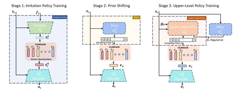
Figure 2. The Framework overview of NCP consists of three stages of training. The first stage involves imitating lifelike movements from unstructured motion clips. In the second stage, a neural categorical prior is trained using prior distillation and adapted using prior shifting to balance different movements. In the final stage, the upper-level policy is trained under the KL-divergence constraint to remain close to the previously trained categorical prior.

Overall, VQ-VAE provides a powerful framework for learning discrete representations of data, which can be used for a variety of tasks, including compression, generation, and clustering.

4. OVERVIEW

Fig. 2 provides an overview of the proposed NCP framework, which is composed of three stages of training described in the rectangles. In the first stage, we use deep RL to initially track and imitate life-like movements from unstructured motion clips using the conditional discrete information bottleneck structure, adapted from that of VQ-VAE. In the second stage, we utilize a prior distillation method to train a neural categorical prior, and then adapt it using a technique named prior shifting to flatten the distribution over distinct states. The shifted categorical prior network is later used for rolling out random trajectories and regularizing the upper-level controllers. At the final stage, we train the upper-level policy under the KL-divergence constraint to let it stay close to the previously trained categorical prior. In the following subsections, we will detail each of these stages.

5. The IMITATION POLICY

Most existing methods of learning reusable motion priors adopt an encoder-decoder architecture or adversarial generative fashion. Both VAE- and GAN-based models have been widely investigated for training an imitation policy given expert demonstrations. As introduced previously, each category of these approaches bears certain limitations. Since the VQ-VAE model belongs to the VAE families, in this section, we first discuss VAE-based methods in detail. Then, we propose the control policy using the discrete information bottleneck to imitate motion clips.

5.1. Limitations of VAE-based Methods

For VAE-based models, one common choice for the prior distribution $p(z)$ is the standard multivariate normal distribution $\mathcal{N}(0,I)$. For instance, (Yao et al., 2022; Won et al., 2022) employ a conditional $\beta$-VAE (Higgins et al., 2017) to imitate motion skills, where the prior is formulated as a conditional distribution $p\left(z_{t}|s_{t}\right)\sim\mathcal{N}(0,I)$. The following loss function is used to train the conditional VAE

(1) $$\mathcal{L}_{\beta\text{-VAE}}=\mathcal{L}_{\text{rec}}+\beta\cdot D_{KL}\left(\mathcal{N}\left(\mu_{t},\sigma_{t}\right)\|\mathcal{N}(0,I)\right)$$

where $\mathcal{L}_{\text{rec}}$ is the reconstruction loss, which measures the difference between the generated character state and target state in motion clips; $D_{KL}(\cdot\|\cdot)$ measures the KL-divergence of the prior distribution $\mathcal{N}(0,I)$ and posterior distribution $\mathcal{N}\left(\mu_{t},\sigma_{t}\right)$ with $\mu_{t}$ and $\sigma_{t}$ being estimated. The parameter $\beta$ controls the strength of the regularization term and trades off between reconstruction accuracy and latent space regularization. The information from the motion clips is compressed into the latent variable $z$, forming an information bottleneck structure.

However, it is difficult to preserve both sample quality and distribution constraint through a compact latent space using $\beta$-VAE. That is, if $\beta$ is too large, excessive penalty on the KL-divergence could lead to posterior collapse, i.e., the KL-vanishing problem (Shao et al., 2020). On the opposite, loosing the KL-divergence could enhance the reconstruction performance, but it might cause the posterior distribution to deviate from the prior distribution, making it challenging to draw samples from the prior distribution.

5.2. Conditional Discrete Information Bottleneck

In this section, we introduce the discrete information bottleneck into an imitation policy. Our imitation policy contains a conditional encoder-decoder structure. The encoder $p^{e}\left(z_{t}^{e}|s_{t},f_{t}\right)$ takes input the state $s_{t}$ and the future trajectory $f_{t}$ from motion clips, and map them to a latent variable $z_{t}^{e}$. The variable $z_{t}^{e}$ will be quantized to an embedding $z_{t}^{q}$ from a finite number of trainable embeddings, which are referred to as codes. The decoder $\pi^{d}(a_{t}|s_{t},z_{t}^{q})$ takes input the state $s_{t}$ and the code $z_{t}^{q}$, and outputs $a_{t}$ as the motor primitive action, i.e., the target joint positions for PD controllers.

The trainable latent embedding codebook is represented as $\mathbf{e}\in R^{K\times D}$, where $K$ is the size of the discrete latent space or the number of codes, and $D$ is the dimensionality of each latent embedding vector or code $e_{i}$, resulting in $K$ embedding vectors $e_{i}\in R^{D},i\in 1,2,\ldots,K$. Given the codebook $\mathbf{e}\in R^{K\times D}$, the encoder output $z_{t}^{e}$ is mapped to the nearest code in $\mathbf{e}$. That is, the discrete latent variables $z_{t}^{q}$ is calculated through the nearest neighbor look-up as denoted below

(2) $$z_{t}^{q}=e_{k},\text{ where }k=\arg\min_{j}\left\|z_{t}^{e}-e_{j}\right\|_{2}.$$

In other words, the posterior categorical distribution $q(\mathbb{I}(z^{e}))$ of the embedding vector index is defined as follows

(3) $$q(\mathbb{I}(z^{e})=k)=\begin{cases}1&\text{ if }k=\underset{j}{\arg\min}\left\|z^{e}-e_{j}\right\|_{2},\\ 0&\text{ otherwise. }\end{cases}$$

where $\mathbb{I}(z^{e})$ is an indicator function returning the index of the selected code for encoding $z^{e}$.

5.3. Latent Space Analysis

We discuss the benefits of using discrete information bottleneck. As revealed in (Roy et al., 2018; Bishop and Nasrabadi, 2006), the quantization process of VQ-VAE, the K-means, and the EM algorithm share many similarities. Considering a Gaussian mixture model with means $\mathbf{e}$ and covariance matrices $\epsilon\mathbf{I}$ of the mixture components, where $\epsilon$ is a shared variance parameter for all of the components. Give a particular data point $z^{e}$, the posterior probability of $\mathbb{I}(z^{e})$ can be formulated using the EM algorithm as follows

(4) $$q(\mathbb{I}(z^{e})=k)=\frac{\delta_{k}\exp\left\{-\left\|z^{e}-e_{k}\right\|^{2}/2\epsilon\right\}}{\sum_{j}\delta_{j}\exp\left\{-\left\|z^{e}-e_{j}\right\|^{2}/2\epsilon\right\}},$$

where $\delta_{k}$ is the prior probability of the $k$-th component of the mixture. If we consider the limit $\epsilon\rightarrow 0$, as shown in (Bishop and Nasrabadi, 2006), the term $\delta_{j}\exp\left\{-\left\|z^{e}-e_{j}\right\|^{2}/2\epsilon\right\}$ for which $\|z^{e}-e_{j}\|^{2}$ is smallest will go to zero most slowly. Therefore, all terms in the posterior distribution approach zero except for one term, which approaches 1. This reveals in this extreme setting, the data point $z^{e}$ is assigned to a cluster in a hard manner, demonstrating the same process as described in Eq. (3). So, the latent distribution of the discrete information bottleneck is actually a multivariate Gaussian mixture model with covariance matrices $\epsilon\mathbf{I}$, where $\epsilon$ is close to 0. This provides theoretical evidence to support that the discrete information bottleneck is likely to achieve superior performance when utilizing finite discrete latent variables.

On the other hand, the discrete bottleneck can lead to a compact latent space. In contrast to the original VQ-VAE, which selects a set of embeddings for the decoder (where each embedding corresponds to a pixel of image in their case), our framework utilizes only a single embedding that is passed to the decoder. Therefore, the discrete information bottleneck yields a compressed yet interpretable latent space consisting of $K$ discrete points in continuous space, as opposed to the continuous latent spaces of VAE- and GAN-based methods. The usage of discrete spaces can offer significant advantages for downstream tasks. In particular, exploration in discrete space could be much easier compared to exploration in continuous space, as discussed in several previous works (Tang and Agrawal, 2020; Andrychowicz et al., 2020).

Moreover, VQ-VAE has the advantage of applying a constant KL-divergence between the prior and posterior distributions, avoiding the need to balance the reconstruction loss and KL-divergence as considered in previous $\beta$-VAE based works. This property makes the training process simpler and more stable.

5.4. Training

To enable a single control policy to imitate all motion clips, our framework employs a tracking-based way. Unlike (Yao et al., 2022; Won et al., 2022), who train a world model to construct a complete VAE to reconstruct the states, we follow the tracking method proposed in (Peng et al., 2018), which defines some imitation rewards and use RL to train the model. In our case, the reward $r_{t}$ is defined as

(5) $$r_{t}=\left\|\mathbf{W}^{1/2}\Omega(s_{t+1}-s_{t+1}^{*})\right\|_{2}^{2},$$

where $\mathbf{W}$ is a diagonal weight matrix selected based on empirical evidence to balance the magnitude of each imitation reward; $\Omega(s)$ is a function specifically designed to determine the reward associated with a given state difference. The subsequent target state in motion clips is represented as $s_{t+1}^{*}$, and state $s_{t+1}$ represents the actual next arrived state calculated by the simulator. Using RL, we can accurately imitate of a broad range of motion clips.

Similar to Eq. (1), the loss in our framework also composes of two parts, an RL objective to imitate the movements in motion datasets and a commitment loss to learn a powerful latent representation. The overall objective is formulated as

(6) $$\begin{gathered}\underset{\theta,\phi,e}{\text{maximize}}\ \mathbb{E}_{p_{\theta}^{e},\pi_{\phi}^{d}}\bigg{[}\sum_{t=0}^{T-1}\Big{(}\gamma^{t}r_{t}-\left\|\operatorname{sg}\left[z_{t}^{e}\right]-e\right\|_{2}^{2}-\beta\left\|z_{t}^{e}-\operatorname{sg}[e]\right\|_{2}^{2}\Big{)}\bigg{]}\end{gathered}$$

where $\theta$ and $\phi$ are the parameters of the encoder $p^{e}$ and decoder $\pi^{d}$, respectively; $\operatorname{sg}$ indicates the stopgradient operator, which is defined as an identity during forward computation and has partial derivatives that equal to zero; the notation $e$ without any indexing indicates the nearest neighbor look-up from the codes; according to (Van Den Oord et al., 2017; Razavi et al., 2019), $\beta$ is a quite robust parameter in balancing the two terms in the commitment loss.

5.5. Prioritized Sampling

We propose to imitate all motion clips into a single policy. Similar to the data imbalance issue commonly encountered in standard supervised learning, some motion clips that are rare from the dataset might be underfitting in the imitation policy. For example, some agile movements like the combination of punches are captured less frequently compared to common locomotion behaviors like walking. Worse still, due to the dynamics, these agile movements are usually more challenging to imitate than other motion clips. The consequence is that the imitation policy fails to reproduce such movements. Instead of uniformly sampling motion clips in the dataset, we utilize prioritized sampling, where the motion clip $m_{i}$ from the dataset $\mathcal{M}$ is sampled with probability

(7) $$p_{i}=\frac{f(R_{m_{i}})}{\sum_{m\in\mathcal{M}}f(R_{m})},$$

where $f:[0,1]\rightarrow[0,\infty)$ is a weighting function and $R_{m}\in[0,1]$ represents the normalized rewards obtained in the RL tracking task for motion clip $m$.

By choosing $f(x)=(1-x)^{\alpha_{1}}$, the policy keeps attention on these challenging motion clips. The sharpness of the distribution can be determined by choosing $\alpha\in\mathbb{R}_{+}$. Similar practices have been reported in (Xie et al., 2022; Won and Lee, 2019).

6. PRIOR

When reusing the pre-trained representation in downstream tasks, existing VAE-based methods often discard the trained encoder in the previous stage, and directly create a upper-level policy to explore the latent space to drive the fixed decoder. In fact, the encoder contains valuable information from the original data distribution. In this section, we explain how to make use of the encoder $p^{e}(z_{t}^{e}|s_{t},f_{t})$ learned in the imitation stage to learn a prior distribution. This prior can then be used to generate a variety of motions and facilitate downstream task learning.

6.1. Prior Distillation

Similar to VQ-VAE, a constant and uniform prior is kept during the training of the imitation policy. After that, we additionally train a categorical prior network $\pi_{\varphi}^{p}(\cdot|s_{t})$ with parameter $\varphi$ to fit the categorical distribution over the codes given only $s_{t}$, without knowing the future trajectory $f_{t}$. We formulate this process as a policy distillation problem (Rusu et al., 2015). That is, we fit the distribution of the encoder’s output $z^{e}$ using $\pi_{\varphi}^{p}(\cdot|s_{t})$ with parameter $\varphi$. In this fitting process, we collect trajectories using the current $\pi_{\varphi}^{p}(\cdot|s_{t})$, and the trajectories are used to optimize the following distillation objective

(8) $$\underset{\varphi}{\text{minimize}}\ \mathbb{E}_{\tau\sim\pi_{\varphi}^{p},\atop f_{t}\sim\mathcal{M}}\ \sum_{t=0}\mathrm{KL}\left(p_{\theta}^{e}(\cdot|s_{t},f_{t})\|\pi_{\varphi}^{p}(\cdot|s_{t})\right),$$

where $\tau$ is the trajectory generated by the prior network $\pi_{\varphi}^{p}$ and $f_{t}$ is some future trajectory randomly sampled from the motion dataset $\mathcal{M}$. This process is repeated iteratively until convergence of the prior network. The trained prior networks can be used to generate random naturalistic movements following the original data distribution. More explanations for expanding Eq. (8) can be found in the Appendix C.

6.2. Prior Shifting

After the prior distillation process, sampling a sequence of codes from the distribution $\pi_{\varphi}^{p}(\cdot|s_{t})$ allows the decoder to execute high-quality movements. However, due to the data imbalance of $\mathcal{M}$ in the prior distillation process, sampling codes from the trained prior distribution naturally drive the decoder to perform movements that appeared more frequently in the data. This could raise diversity issues when the data is imbalanced.

To facilitate the exploration in downstream task learning with unknown skill preference, it is desired to have a balanced prior capable of performing a diverse range of movements with nearly uniform probability over distinct motions in the dataset. Inspired by the curiosity-driven exploration methods (Strehl and Littman, 2008; Ostrovski et al., 2017; Bellemare et al., 2016), we propose a count-based RL method to fine-tune the prior distribution.

In prior shifting, the prior network is initialized from the distillation stage and the decoder is fixed. The latent variables sampled from the prior drive the decoder to generate movements. To adjust the prior distribution, we employ a heuristic count-based reward defined as

(9) $$r(s)=\sqrt{\frac{N_{k}}{\hat{N}(s)}}$$

where $\hat{N}(s)$ is a pseudo-count of a continuous state $s$, and $N_{k}$ is a constant used to scale the magnitude of the reward. To estimate the pseudo-count $\hat{N}(s)$ in continuous space, density models have been applied in existing works such as (Ostrovski et al., 2017; Bellemare et al., 2016). In our case, considering the limited number of frames in motion clips, we estimate the pseudo-count by simply using a motion matching method without the need for precise density model fitting. To achieve this, a metric is defined to select motion frames in motion clips that are close to the sampled data within a given threshold, and the count of every matched frame is increased by 1 and stored in a table with a size being equal to the number of frames. To stabilize the training, only the latest $T_{k}$ generated states are counted, where $T_{k}$ is a constant. The reward is then calculated using the count of the frame with the highest matching score. In cases where a state is unable to match any frame in the dataset given the threshold, we assign a zero reward to penalize unnatural behaviors.

7. UPPER-LEVEL POLICY

Now, we are ready to solve downstream tasks. The pre-trained decoder $\pi_{\phi}^{d}$ and shifted prior distribution $\pi_{\varphi}^{p}$ have absorbed sufficient knowledge on both movement quality and diversity. Reusing these pre-trained networks, the remaining job is simply building an upper-level policy $\pi_{\vartheta}^{h}(\cdot|s_{t},g_{t})$ with parameter $\vartheta$ for choosing a discrete code to drive the fixed decoder for producing actions, where $g_{t}$ indicates some task-specific goals that are only relevant to the downstream tasks. Below, we introduce how to reuse the shifted prior $\pi_{\varphi}^{p}$ for training the upper-level policy $\pi_{\vartheta}^{h}$.

7.1. KL-Regularized Training

Specifically, in addition to the RL loss that maximizes the cumulative task reward, we apply a KL-regularized term to ensure that the upper-level policy $\pi_{\vartheta}^{h}$ remains close to the pre-trained prior distribution $\pi_{\varphi}^{p}$. Moreover, an entropy bonus term is also incorporated to promote exploration and prevent convergence to sub-optimal solutions. The loss function is formulated as follows

(10) $$\begin{split}\text{maximize}_{\vartheta}\ \mathbb{E}_{\pi_{\vartheta}^{h}}\left[\sum_{t=0}\gamma^{t}r_{t}\right]&-\alpha_{\mathrm{KL}}\cdot\mathrm{KL}\left(\pi_{\vartheta}^{h}(\cdot|s_{t},g_{t})||\pi_{\varphi}^{p}(\cdot|s_{t})\right)\\ &+\alpha_{\mathrm{H}}\cdot\mathrm{H}(\pi_{\vartheta}^{h}),\end{split}$$

where $r_{t}$ here indicates the downstream task reward and $\mathrm{H}(\pi_{\vartheta}^{h})$ is the entropy. This objective aims to maximize rewards while letting the upper-level policy stay close to the learned prior to performing movements in motion clips. Therefore, it encourages exploration and prevents the policy from converging to a deterministic solution, which promotes the learning of multiple solutions to a task to enhance diversity.

7.2. Prioritized Fictitious Self-Play

In the experiments, we will evaluate the proposed method in a two-player boxing game. We are curious about how well an upper-level policy can reach by reusing the proposed NCP in a real-life sports game. To fulfill this, we employ prioritized fictitious self-play (PFSP) which has been demonstrated as a very effective multi-agent RL method in producing strong game AIs (Vinyals et al., 2019; Han et al., 2020).

In PFSP, we launch parallel games, in each of which the current training agent and a historically dumped version of its policy parameters are chosen to perform a boxing game. For every certain training iteration (around an hour), a copy of the agent’s policy parameters is dumped and added to a candidate set of historical policies. At the beginning of a new game, the probability of sampling a historical policy $i$ from the candidate set $\mathcal{O}$ is given by:

(11) $$p_{i}=\frac{g(P_{i})}{\sum_{o\in\mathcal{O}}g(P_{o})},$$

where $g:[0,1]\rightarrow[0,\infty)$ is a weighting function and $P_{o}\in[0,1]$ denotes the probability that the agent can defeat the policy $o$. Similar to Section 5.5, we also choose $g(x)=(1-x)^{\alpha_{2}}$. Under this setup, the current player tends to choose the most challenging opponents in priority from the candidate set.

8. RESULTS

We evaluate the proposed framework on two benchmark motion datasets (Peng et al., 2022; Won et al., 2021). We aim to verify the following statements: 1) our framework can learn a compact and informative latent representation that allows the characters to perform diverse and sophisticated movements, while maintaining realistic motion from the unstructured motion clips; 2) the shifted prior can generate various random trajectories covering the majority of the motions demonstrated in motion clips; 3) the upper-level policy can effectively reuse the pre-trained representation and prior distribution to solve new downstream tasks, including both single-agent task and two-player zero-sum game.

8.1. Experimental Setup

The simulation environments are implemented using the Isaac Gym simulator (Makoviychuk et al., 2021) with a simulation frequency of 120Hz, where the control policies execute at a frequency of 30Hz. To demonstrate the generality of our framework, we evaluated it on two different humanoid characters: one equipped with a sword and a shield with 37 degrees-of-freedom, similar to the character used in (Peng et al., 2022). Another character is equipped with boxing gloves with 34 degrees-of-freedom, similar to the character used in (Won et al., 2021). The imitation policy for the sword & shield character is trained on a total of approximately 26 minutes of motion data, consisting of 82 motion clips from (Peng et al., 2022) for moving and stunt motions, and 76 locomotion motion clips. For the boxer character, 45 boxing and locomotion motion clips from http://mocap.cs.cmu.edu and http://mocap.cs.sfu.ca with their mirrored data are used, approximately 30 minutes in total.

All experiments are implemented on NVIDIA TESLA P40 GPUs under TLeague (Sun et al., 2020), an efficient distributed multi-agent RL infrastructure. We use proximal policy optimization (PPO) (Schulman et al., 2017) as the RL algorithm. For detailed hyperparameters, please refer to Section A in Appendix. Both the imitation tasks for the sword & shield character and boxer character take around 2 days of training. The prior training requires 12 hours. The strike task can be accomplished within 4 hours, while the boxing task demands 4 days to converge.

8.2. Setup and Results for Imitation Policy

8.2.1. States

In our framework, the state $s_{t}$ characterizes the proprioceptive observation of the character, which is defined as

(12) $$s_{t}=\left\{q_{j},\dot{q}_{j},p_{i},q_{i},v_{i},\omega_{i},h\right\},$$

where $q_{j}$ and $\dot{q}_{j}$ are the joint position and joint velocity of the $j$-th joint, respectively; $p_{i}$, $q_{i}$, $v_{i}$ and $\omega_{i}$ are the relative position, orientation, the linear and angular velocity of the $i$-th body expressed in the local coordinate frame of the root; $h$ represents the height of the root relative to the ground. The orientation is represented using a 6D vector (Zhou et al., 2019). In addition to the current proprioceptive observation, the imitation policy additionally takes input the future information vector $f_{t}$, which represents the future states of the character in motion clips. In our experiment, we define $f_{t}=\left\{\delta\left(s_{t},s_{t+1}^{*}\right),\delta\left(s_{t},s_{t+2}^{*}\right)\right\}$ to allow the imitation policy to receive the information of the subsequent two frames in motion clips. $\delta\left(s_{t},s_{t}^{*}\right)$ is a function that measures some key information in the state $s_{t}$ and a target state $s_{t}^{*}$. It is defined as

(13) $$\delta\left(s_{t},s_{t}^{*}\right)=\left\{q_{j}^{*},\dot{q}_{j}^{*},p_{r}^{*},q_{r}^{*},v_{r}^{*},\omega_{r}^{*},p_{k}^{*}\right\},$$

where $q_{j}^{*}$ and $\dot{q}_{j}^{*}$ are target joint position and joint velocity of the $j$-th joint expressed in datasets; $p_{r}^{*}$, $q_{r}^{*}$, $v_{r}^{*}$, and $\omega_{r}^{*}$ are the relative position, orientation, linear and angular velocity of the target state expressed in the simulated character root coordinate frame; $p_{k}^{*}$ represents the position of certain key body parts of the target state represented in the target root coordinate frame. The key body parts for the boxer character are the hands and feet, while the other character utilizes both their hands and feet as well as a sword and shield.

The character with sword & shield has a state $s_{t}$ with 362 dimensions and a future information vector $f_{t}$ with 284 dimensions to include information about the sword and shield, while the boxer character receives a state $s_{t}$ with 323 dimensions and a future information vector $f_{t}$ with 254 dimensions.

8.2.2. Actions

The characters are immediately controlled by the output of the PD controllers, i.e., the torques. The control policies output target positions of the joints, which are fed into the PD controllers. To alleviate the burden of exploration, the action $a_{t}$ serves as a residual target position. The target joint position $\hat{q}_{t}$ is calculated by adding the action vector $a_{t}$ to the current joint position $q_{t}$, i.e., $\hat{q}_{t}=q_{t}+a_{t}$. The character with sword & shield has an action space with 31 dimensions, while the boxer character has an action space with 28 dimensions.

8.2.3. Latent

The codebook $e\in R^{K\times D}$ serves as the latent representation, where $D$ is the dimensionality of latent embedding vector $e_{i}$, and $K$ is the number of latent embedding vector. Throughout our experiments, we set $D=64$. For the character with sword & shield, we set $K=512$, and we set $K=256$ for the boxer character.

8.2.4. Network Architecture

For the implementation of RL, we use the actor-critic infrastructure with PPO algorithm. Therefore, we need to train a policy (containing the encoder and decoder) for the actor and a value function for the critic. The value function, encoder and decoder are all parameterized as deep neural networks. The value function $V(s_{t},f_{t})$ is modeled with a fully connected network with 3 hidden layers of $[1024,512,256]$ units. For the policy network, the encoder takes in state $s_{t}$ and $f_{t}$, and maps them to a latent variable $z_{t}^{e}$ using a fully connected network with 3 hidden layers of $[1024,1024,512]$ units. The latent $z_{t}^{e}$ is quantized to $z_{t}^{q}$, and the decoder takes in state $s_{t}$ and $z_{t}^{q}$ and maps them to a Gaussian distribution with a mean $\pi^{d}(a_{t}|s_{t},z_{t}^{q})$ and a trainable diagonal covariance matrix $\Sigma_{\pi}$. The decoder is also modeled with a fully connected network with 3 hidden layers of $[1024,1024,512]$ units.

8.2.5. Reward

For the imitation policy, an objective similar to (Peng et al., 2018) is employed in our framework to track motion clips. The objective is

(14) $$r_{t}=w^{jp}r_{t}^{jp}+w^{jv}r_{t}^{jv}+w^{k}r_{t}^{k}+w^{r}r_{t}^{r}+w^{v}r_{t}^{v}$$

where $r_{t}^{jp}$, $r_{t}^{jv}$, $r_{t}^{k}$, $r_{t}^{r}$, and $r_{t}^{v}$ correspond to the tracking reward of joint angles, joint velocities, key body, root, and root velocity, respectively. The weight of each reward is denoted as $w$ with the same superscript. See Section B in Appendix for detailed information on reward settings.

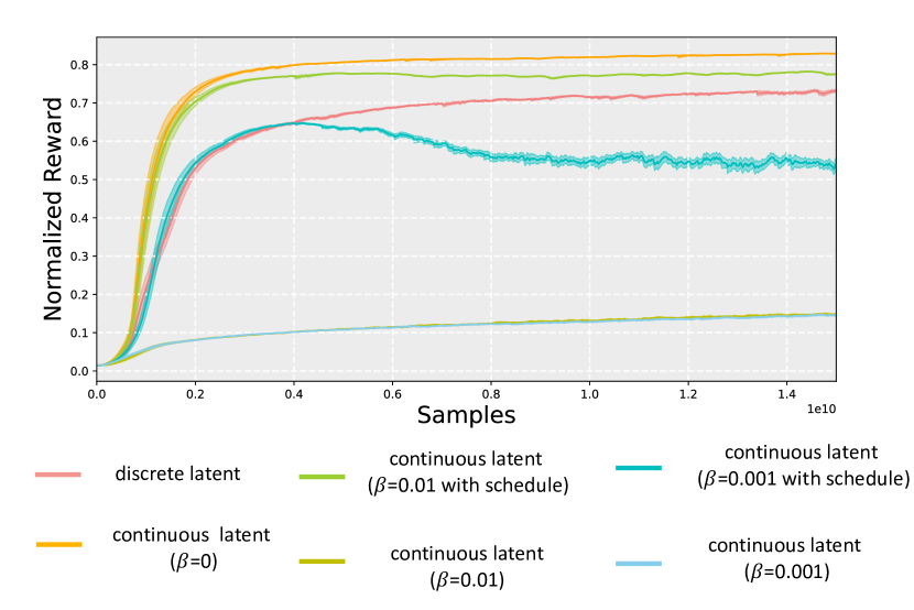
Figure 3. Learning curves of various $\beta$-VAE variants and ours (denoted as discrete latent).

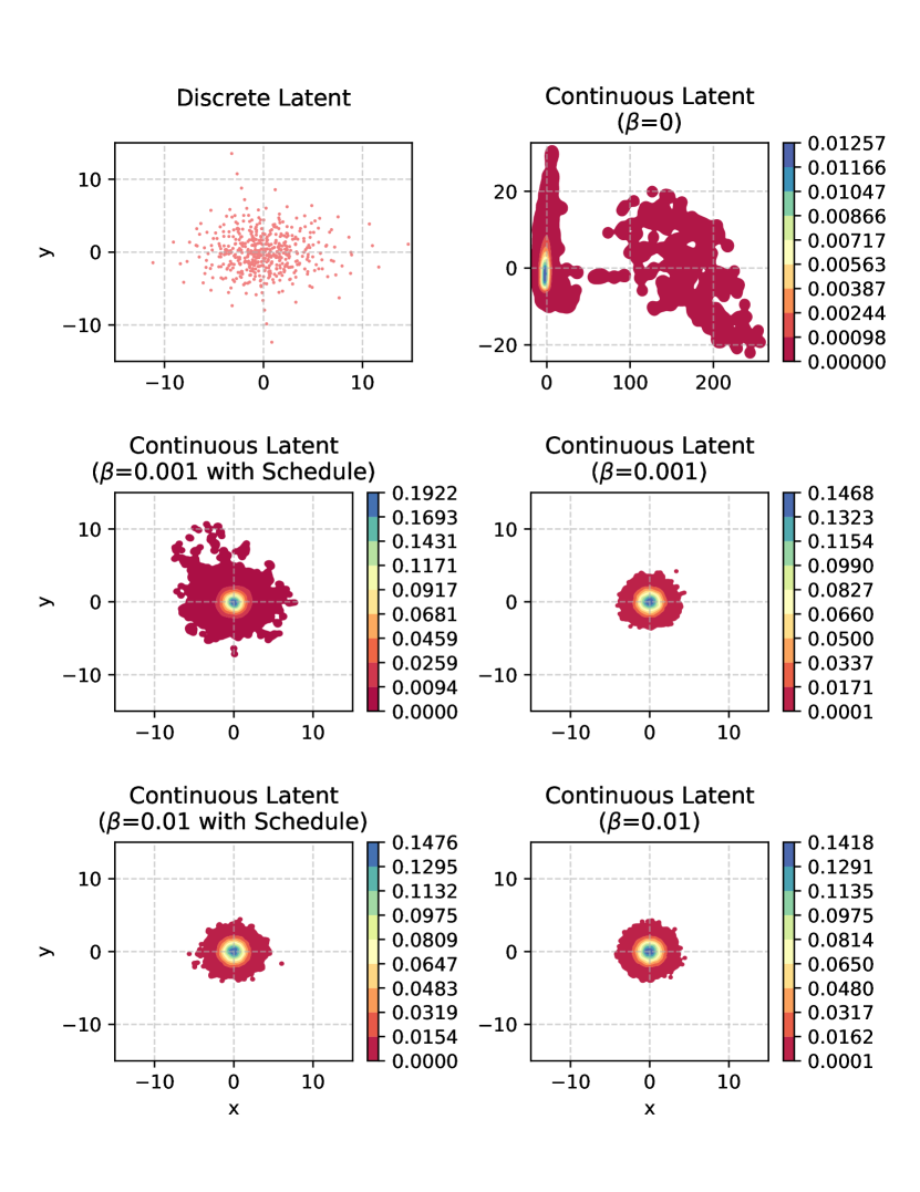
Figure 4. Visualization of discrete and continuous latent distributions from various methods using Principal Component Analysis (PCA). For the continuous latent distribution, Kernel Distribution Estimation (KDE) is employed to estimate the distribution.

.

8.2.6. Evaluation

We train each humanoid character with an imitation policy. The results show that each character is able to perform sufficiently diverse and realistic movements, including locomotion, boxing, and sword & shield stunts. To quantitatively analyze the effectiveness of the imitation policy, we use the sword & shield dataset and conduct comprehensive comparative experiments with VAE-based- and GAN-based methods below.

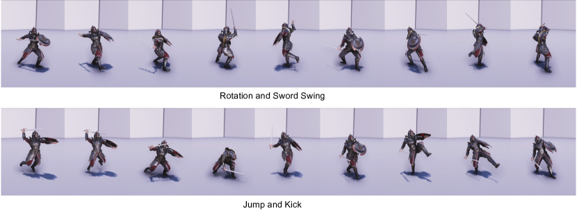
Figure 5. The tracking performance of the imitation policy of NCP for the character with sword & shield.

test

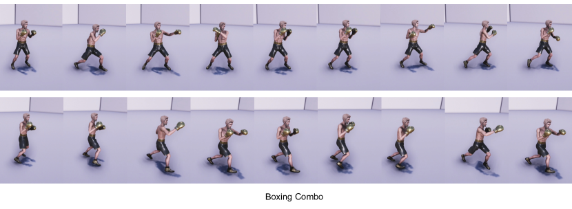
Figure 6. The tracking performance of the imitation policy of NCP for the boxer character.

test

Comparison with VAE-based methods. We compare with a number of $\beta$-VAE variants with different settings on $\beta$ in Eq. (1). Specifically, we test $\beta=0.01$ and $\beta=0.001$ with and without the annealing schedule trick, resulting in 4 $\beta$-VAE candidates. Despite those, we additionally consider an extreme case with $\beta=0$. For a fair comparison, for these $\beta$-VAE variants we use similar neural network architecture as ours and the dimension of their latent variable $z$ is set to $64$ as well. The reward curves comparing the tracking performance of all candidates are shown in Fig 3. At the same time, we would like to understand the expressive power of the latent representations for different methods, since VAE-based methods including ours try to seek for a balance between the reconstruction quality and the compatibility of the latent distribution with a prior. To understand the latent space, we plot the 64 dimensional latent variables for all the compared methods on a 2D space using Principal Component Analysis (PCA). The visualization of the 2-dimensional latent is shown in Fig. 4.

From Figs. 3 and 4, as expected, the $\beta=0$ variant shows the best tracking performance, since the latent space is not regularized; however, its latent distribution is broad and apparently not reusable for action generation. For $\beta=0.01$ and $\beta=0.001$, both variants cause posterior collapse, resulting in latents that are close to the standard Gaussian distribution while they fail to track the motion clips. On the other hand, the annealing schedule (Bowman et al., 2015) trick is verified effective in preventing posterior collapse, using which $\beta$ linearly increases from 0 to 0.01 or 0.001 during training. The according two variants with annealing schedule achieve a relatively compact latent space and maintain a relatively good tracking performance.

The empirical results on the continuous latent space demonstrate again that increasing $\beta$ could produce a compact latent space, but ultimately lead to deteriorated tracking performance, while decreasing $\beta$ can enhance tracking performance but lead to a widely distributed latent distribution, making it challenging for upper-level policy usage. Therefore, it is not trivial for VAE-based methods to reach a perfect balance.

Now, we discuss the performance of our proposed method. According to Fig. 3, the tracking performance of the proposed method is slightly lower than the $\beta=0$ VAE variant and $\beta=0.001$ with annealing schedule variant. As demonstrated in the videos, such tracking performance is sufficient to produce high-quality movements. For the learned latent space, it is obvious in Fig. 4 that our method produces a discrete latent space with the scattered codes indicating the means of multiple Gaussians. The codes span over the 2D space and provide a broad yet compact distribution, since the discrete space is quite small, with only $256$ / $512$ codes for the boxer / sword & shield character. Unlike VAE, the discrete latent space considerably facilitates upper-level usage. For the case of upper-level RL, it alleviates the exploration burden of the upper-level policy, compared to exploring in a continuous Gaussian space.

Comparison with GAN-based methods. Recent developments in GAN-based methods have shown impressive results in generating high-quality skills for physics-based characters. To showcase the effectiveness of our framework, we compare our results with the state-of-the-art approach ASE (Peng et al., 2022) and CALM (Tessler et al., 2023) using the same motion datasets. Both ASE (Peng et al., 2022) and CALM (Tessler et al., 2023) have released the trained model parameters, and hence we direct evaluate on these models without any bias. To achieve a fair comparison, we first generate approximately one million data in $\mathcal{F}$ by randomly sampling from the latent space of each method in ASE, CALM, and our NCP, separately. Then, we define a general reconstruction score $s(f_{i}^{*})$ for frame $f_{i}^{*}$ in motion clips as

(15) $$s(f_{i}^{*})=\underset{f\in\mathcal{F}}{\max}\quad 0.5\cdot r^{jp}(f_{i}^{*},f)+0.5\cdot r^{v}(f_{i}^{*},f),$$

where $r^{jp}(f_{i}^{*},f)$ and $r^{v}(f_{i}^{*},f)$ are defined identically as in Eq. (14). $r^{jp}$ and $r^{v}$ measure the similarity of joint position and root velocity between frame $f_{i}^{*}$ stored in motion clips and frame $f$ sampled from the decoder of each method. Note that none of the ASE, CALM and ours directly optimize the above score, and the score is general to evaluate the performance of generated motions from various control policies.

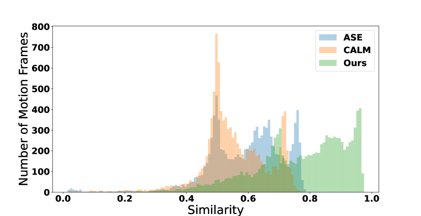
Figure 7. Comparison of reconstruction similarity scores of ASE, CALM, and our method.

.

The above reconstruction scores for different methods are evaluated in Fig. 7, where the $y$-axis indicates the number of motion frames and the $x$-axis indicates the computed reconstruction similarity score. Intuitively, more motion frames falling in the interval with higher scores indicate better reconstruction performance and motion coverage. That is, the histogram area centered at the right-hand side indicates better performance. As observed in the figure, CALM exhibits better diversity and tracking performance compared to ASE, and this is consistent with the conclusion in (Tessler et al., 2023); while our model produces significantly more naturalistic and diverse behaviors compared to both ASE and CALM. This conclusion can also be obviously observed from the videos in the supplementary materials. Furthermore, we count the number of frames that obtain a reconstruction score above 0.5 and compute the ratio over the total number of training frames. Our approach achieved a rate of 94.6%, whereas ASE achieved 77.1% and CALM achieved 69.6%.

Finally, we screenshot a few frames of the simulated characters when tracking the motion clips in Figs. 5 and 6. As shown in these images, both the characters can perfectly reproduce some complex movements in the motion clips, such as rotation, sword swing, jumping and kicking movements for the sword & shield character, and combination of punches for the boxer character.

8.3. Setup and Results for Prior

8.3.1. Observation and Action

In our framework, the prior only takes proprioceptive observation $s_{t}$ of the character as input, as defined in Eq. (12). The action space of the prior is the categorical distribution over the codes. In the case of the sword & shield character, the action is represented as a 512-dimensional vector, i.e., the code, while for the boxer character, it is a 256-dimensional vector.

8.3.2. Network Architecture

During the training of prior, both the value function and policy function are modeled using fully connected neural networks. The value function consists of three hidden layers with 1024, 512, and 256 units, respectively. Similarly, the policy function is modeled using three hidden layers, consisting of 1024 units in each layer.

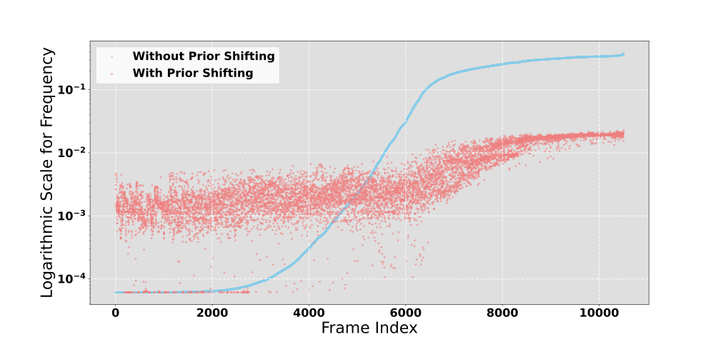
Figure 8. Comparison of frame visit frequency between without prior shifting and with prior shifting for the character equipped with sword & shield.

.

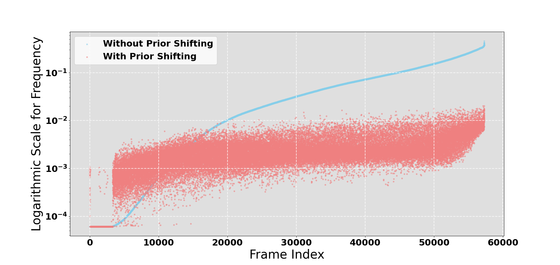
Figure 9. Comparison of frame visit frequency between without prior shifting and with prior shifting for the boxer character.

.

8.3.3. Evaluation

In this section, we evaluate the effectiveness of the proposed prior shifting technique. Since prior shifting is introduced to produce more diverse behaviors, we perform statistics on the generated movements by randomly sampling codes from the priors with and without prior shifting.

Figs. 8 and 9 show the comparison of frame visitation frequencies (with log scale) of using and not using the prior shifting for the sword & shield character and boxer character, respectively. The frames along the $x$-axis are sorted by their visitation frequencies before prior shifting, and hence the blue points show a smooth pattern along the $x$-axis. As we can observe, using prior shifting, the shifted prior distribution is tuned to match a nearly even distribution over all the motion frames. This provides sufficient confidence for reusing this prior in downstream tasks.

8.4. Setup and Results for Upper-Level Policy

8.4.1. Observation and Action

The upper-level policy $\pi_{\vartheta}^{h}(\cdot|s_{t},g_{t})$ takes the proprioceptive observation $s_{t}$ defined in Eq. (12) and a task-specific goal $g_{t}$ as inputs. The goal $g_{t}$ for the strike task is defined similarly to (Peng et al., 2022), using a 15-dimensional vector that represents the relative position, orientation, linear velocity, and angular velocity of the target. While in the boxing task, the goal $g_{t}$ represents the opponent’s state by a 289-dimensional vector that includes the body position, rotation, root linear velocity, and angular velocity of the opponent, expressed in the root coordinate system of the agent. The action space of the upper-level policy is consistent with the prior network which the policy selects a code from the categorical distribution to drive the decoder to generate movements. The action of the sword & shield character is represented by a 512-dimensional vector, while that of the boxer character is a 256-dimensional vector.

8.4.2. Network Architecture

Both the value function and policy function in the upper-level policy are modeled using fully connected neural networks. The value function is composed of three hidden layers with 1024, 512, and 256 units, and the policy function is composed of three hidden layers with 1024, 512, and 512 units, respectively.

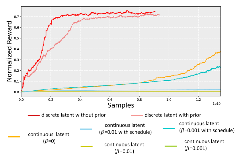
Figure 10. Upper-Level policy learning curve using different decoders.

.

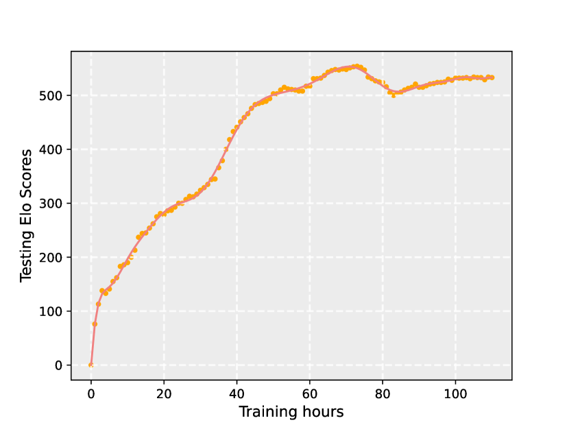
Figure 11. The testing Elo scores of generated players during the PFSP training. Each point represents the score of a trained player along the training time.

test

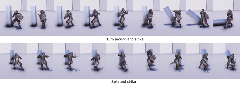
Figure 12. The performance of our method in the strike task.

test

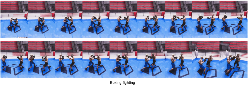
Figure 13. The performance of our method in the two-player boxing game.

test

8.4.3. Reward

The reward function for the strike task is similar to that for  (Peng et al., 2022):

$$r=w_{\text{strike }}r_{\text{strike }}+w_{\text{facing }}r_{\text{facing }}+w_{\text{vel }}r_{\text{vel }},$$

and the strike reward $r_{\text{strike }}$ is defined as

$$r_{\text{strike }}=1-u^{up}\cdot u_{t}^{*},$$

where $u^{up}$ and $u_{t}^{*}$ represent the up vector of the global coordinate and the target object, respectively. The facing reward $r_{\text{facing}}$ is defined as

$$r_{\text{facing }}=\exp(-5\cdot|1-\mathbf{d}\cdot\hat{\mathbf{d}}|),$$

$${\mathbf{d}}=\left(\mathbf{p}_{\mathrm{t}}-\mathbf{p}\right)/\left\|{\mathbf{p}}_{\mathrm{t}}-{\mathbf{p}}\right\|,$$

where $\hat{\mathbf{d}}$ is the facing direction of the character, $\mathbf{p}$ and $\mathbf{p}_{\mathrm{t}}$ are the global position of the character and target separately. The velocity reward $r_{\text{vel}}$ is defined as

$$r_{\mathrm{vel}}=\exp\left(-4\cdot\left|\mathbf{v^{*}}-\mathbf{d}\cdot\mathbf{v}\right|\right),$$

where $\mathbf{v}$ and $\mathbf{v^{*}}$ are the global velocity and the goal velocity of the player, respectively. The weights for the strike, facing, and velocity rewards are represented by $w_{\text{strike }}$, $w_{\text{facing }}$, and $w_{\text{vel }}$, respectively. In our experiments, these weights are set to 0.6, 0.2, and 0.2, respectively.

The reward function for the boxing task is designed similarly to (Won et al., 2021) as

$$r=r_{\text{damage }}+w_{\text{facing }}r_{\text{facing }}+w_{\text{vel }}r_{\text{vel }}+w_{\text{fall }}r_{\text{fall }},$$

and the damage reward $r_{\text{damage }}$ is defined as

$$r_{\text{damage }}=\left\|f_{pl->op}\right\|-\left\|f_{op->pl}\right\|,$$

where $\left\|f_{pl->op}\right\|$ is the contact force between the hands of agent and the opponent to measure the damage of punches against the opponent. Different from (Won et al., 2021), the contact force in our task is clipped between 200N and 1200N, which is a natural range for human boxing players. The facing reward $r_{\text{facing}}$ and velocity reward $r_{\text{vel}}$ are defined similarly to the strike task, with the difference being that the target position is now the opponent’s root position. Additionally, a sparse binary reward $r_{\text{fall}}$ is designed for the agent when the opponent falls down. In our experiment, the weights for $w_{\text{facing }}$, $w_{\text{vel}}$, and $w_{\text{fall}}$ are set to 0.6, 0.4, and 100, respectively.

8.4.4. Evaluation

In the last part of the experiments, we evaluate the performance of our method for solving downstream tasks. As mentioned previously, we consider two tasks that are strike task for the character with sword & shield and two-player boxing game. To support the effectiveness of the pre-trained discrete latent representations and prior networks in promoting the efficiency of upper-level policy training, we propose a few ablation studies here to test the decoders trained from various $\beta$-VAE methods and ours.

The training curves of the upper-level policies using different decoders are reported in Fig. 10 for the strike task. As expected, the results show that using the discrete latent can significantly facilitate and speed up the RL training process. Another conclusion in the curves is that without using the trained prior distribution as a constraint in the KL-regularized term, the policy achieves a slightly higher reward than the KL-regularized version with the prior. This is reasonable because without any constraint, the upper-level policy is free to explore the discrete latent space with a single objective that is maximizing the task reward. However, this might cause the policy fails to perform diverse strategies that can elaborate all movements in the motion clips. This is verified in our videos, where the trained policy with prior regularization demonstrates much more diverse behaviors compared with the one without prior regularization. Fig. 12 shows some screenshots of the strike task, where the character could carry out a diverse set of behaviors to strike the square pillar, compared to the performance of the ASE method (Peng et al., 2022) in the same task.

In the two-player boxing game, we additionally consider a multi-agent RL problem and train the upper-level policy using the PFSP algorithm. The training lasts for around 4.5 days. During this time, we dump the network parameters every hour, and a total number of 110 models are stored. To witness how the training progress proceeds, we evaluate the 110 models with Round Robin tournament and perform 100 matches for each pair of players to compute the final payoff matrix. The Elo scores (Coulom, 2005) (a common metric for measuring the overall performance of a player in Round Robin tournament) are plotted in Fig. 11 and demonstrate that the trained boxer can consistently improve and overcome past models.

Finally, we screenshot some impressive frames of the simulated characters in the two-player boxing game in Fig. 13. Surprisingly, we observe that the character emerges life-like strategies similar to professional human boxers in boxing matches, such as defense and dodge. More details can be seen in the video.

9. DISCUSSION

This paper introduces a novel learning framework that enhances the quality and diversity of physics-based character control beyond current state-of-the-art methods. Our approach employs reinforcement learning (RL) to first track and replicate realistic movements from unstructured motion clip datasets using the discrete information bottleneck. This structure extracts the most pertinent information from motion clips into a compact yet informative discrete latent space. By sampling latent variables from a trained prior distribution, we can generate high-quality lifelike behaviors. However, this prior distribution relies on the original data distribution and could be affected by motion imbalance in the dataset. To address this issue, we further propose a technique called prior shifting to adjust the trained prior using curiosity-driven RL. The shifted distribution offers a nearly even distribution of the generated movements over the motion clips in the dataset. This enables its easy usage in upper-level policy, and even a random upper-level policy can produce ample behavioral diversity.

In future work, we aim to investigate the potential of adapting this framework to environmental changes, such as accommodating additional objects and characters. This could enable us to expand the learned policy to adapt to previously unseen environments. Similar to all data-driven methods, the performance of our system is limited by the size of the training dataset. Besides, enhancing our ability to learn more complex behaviors as well as extending the framework to larger datasets, promise to be a fascinating area for future exploration.

Appendix A hyperparameters

Table 1 lists the hyperparameter settings used for the imitation policy, while Table 2 provides the corresponding hyperparameters for prior shifting. Finally, Table 3 contains the hyperparameters for the upper-level policy.

Table 1. Hyperparameters for training imitation policy.

Hyperparameter	Value
Number of Code $K$	512 or 256
Code Dimension $D$	64
Commitment Penalty $\beta$	0.25
GAE($\lambda$)	0.95
Discount Factor $\gamma$	0.95
Policy/Value Function Learning Rate	0.00005
Policy/Value Function Minibatch Size	16384
PPO Clip Threshold	0.1
Prioritized Sampling Coefficient $\alpha_{1}$	3

Table 2. Hyperparameters for prior shifting.

Hyperparameter	Value
Number of Counted States $T_{k}$	4915200
Reward Scale Factor $N_{k}$	$2\times\log(T_{k})$
GAE($\lambda$)	0.95
Discount Factor $\gamma$	0.95
Policy/Value Function Learning Rate	0.00001
Policy/Value Function Minibatch Size	4096
PPO Clip Threshold	0.1

Table 3. Hyperparameters for training upper-level policy.

Hyperparameter	Value
KL Loss Weight $\alpha_{\mathrm{KL}}$	0.05
Entropy Loss Weight $\alpha_{\mathrm{H}}$	0.01
GAE($\lambda$)	0.95
Discount Factor $\gamma$	0.95
Policy/Value Function Learning Rate	0.00005
Policy/Value Function Minibatch Size	8192
PPO Clip Threshold	0.1
PFSP Sampling Coefficient $\alpha_{2}$	2

Appendix B MOTION TRACKING OBJECTIVE

In Section 8.2, we propose that our tracking reward is a weighted sum of specific reward terms. In this section, we provide a description of those terms. The reward $r_{t}$ is defined as

$$r_{t}=w^{jp}r_{t}^{jp}+w^{jv}r_{t}^{jv}+w^{k}r_{t}^{k}+w^{r}r_{t}^{r}+w^{v}r_{t}^{v},$$

$$w^{jp}=0.3,w^{jv}=0.1,w^{k}=0.3,w^{r}=0.2,w^{v}=0.1,$$

The joint angles reward $r_{t}^{jp}$ and joint velocities reward $r_{t}^{jv}$ are defined as:

$$r_{t}^{jp}=\exp\left[-2.0\left(\sum_{j}\left\|q_{t,j}^{*}-q_{t,j}\right\|\right)\right],$$

$$r_{t}^{jv}=\exp\left[-0.1\left(\sum_{j}\left\|\dot{q}_{t,j}^{*}-\dot{q}_{t,j}\right\|\right)\right],$$

where $q_{t,j}$ and $\dot{q}_{t,j}$ represents the joint angle and joint velocity of the j-th joint at time t, while $q_{t,j}^{*}$ and $\dot{q}_{t,j}^{*}$ are the corresponding target joint angle and joint velocity represented in motion clips.

The key body reward $r_{t}^{k}$ is defined to tracking the position of the key body of the agent, which is formulated as follows

$$r_{t}^{k}=\exp\left[-10.0\left(\sum_{k}\left\|p_{t,k}^{*}-p_{t,k}\right\|\right)\right]$$

where $p_{t,k}$ represents the position of the k-th body relative to the root, and $p_{t,k}^{*}$ represents the position in motion clips.

For the root, two types of rewards are defined as

$$r_{t}^{r}=\exp\left[-20.0\left(\left\|p_{t,r}^{*}-p_{t,r}\right\|^{2}+0.5*\theta^{2}\right)\right],$$

$$r_{t}^{v}=\exp\left[-2.0\left(\left\|v_{t,r}^{*}-v_{t,r}\right\|^{2}+0.1*\left\|\omega_{t,r}^{*}-\omega_{t,r}\right\|^{2}\right)\right],$$

where $p_{t,r}$, $v_{t,r}$, and $\omega_{t,r}$ represent the position, linear velocity, and angular velocity of the root, respectively, $p_{t,r}^{*}$, $v_{t,r}^{*}$, and $\omega_{t,r}^{*}$ are the target stored in motion clips. $\theta$ denotes the angle in the axis-angle representation of $R^{*}R^{-1}$, while $R^{*}$ represent the root orientation in motion clips and $R$ is the root orientation of the agent.

Appendix C EXPLANATION of EQUATION (8)

Without loss of generality, $p(\cdot)$ stands for a probability function without other specifications. The probability of the trajectory $\tau$ in Eq. (8) is

$$\pi_{\varphi}^{p}(\tau)=p\left(s_{0}\right)\prod_{t=0}\pi_{\varphi}^{p}\left(k|s_{t}\right)\pi_{\phi}^{d}\left(a_{t}|s_{t},(e_{k})_{t}\right)p\left(s_{t+1}|s_{t},a_{t}\right)$$

where the index $k$ is sampled from the categorical prior network $\pi_{\varphi}^{p}$ and $(e_{k})_{t}$ is the corresponding code $e_{k}$ at time step $t$. Then, Eq. (8) can be derived as

(16) $$\mathbb{E}_{\tau\sim\pi_{\varphi}^{p},\atop f_{t}\sim\mathcal{M}}\ \sum_{t=0}\sum_{z_{t}^{e}\sim p_{\theta}^{e}}p_{\theta}^{e}(z_{t}^{e}|s_{t},f_{t})\log\frac{p_{\theta}^{e}(z_{t}^{e}|s_{t},f_{t})}{\pi_{\varphi}^{p}(\mathbb{I}(z_{t}^{e})|s_{t})}$$

$$= \mathbb{E}_{s,f,z,a\ \sim\atop\rho^{p_{\theta}^{e},\pi_{\varphi}^{p},\pi_{\phi}^{d},\mathcal{M}}}\ -\pi_{\varphi}^{p}(\mathbb{I}(z)|s)\log\pi_{\varphi}^{p}(\mathbb{I}(z)|s),$$

where the equality holds by noting that $p_{\theta}^{e}(z_{t}^{e}|s_{t},f_{t})$ has a probability mass on the nearest code according to Eq. (3); $\rho^{p_{\theta}^{e},\pi_{\varphi}^{p},\pi_{\phi}^{d},\mathcal{M}}$ is a visitation probability commonly used in RL theories. Eq. (16) demonstrates that optimizing the distillation loss acts similarly with the prior fitness in VQ-VAE for unconditioned samples.

References

- (1)
- Andrychowicz et al. (2020) OpenAI: Marcin Andrychowicz, Bowen Baker, Maciek Chociej, Rafal Jozefowicz, Bob McGrew, Jakub Pachocki, Arthur Petron, Matthias Plappert, Glenn Powell, Alex Ray, et al. 2020. Learning dexterous in-hand manipulation. The International Journal of Robotics Research 39, 1 (2020), 3–20.
- Bellemare et al. (2016) Marc Bellemare, Sriram Srinivasan, Georg Ostrovski, Tom Schaul, David Saxton, and Remi Munos. 2016. Unifying count-based exploration and intrinsic motivation. Advances in Neural Information Processing Systems 29 (2016).
- Bergamin et al. (2019) Kevin Bergamin, Simon Clavet, Daniel Holden, and James Richard Forbes. 2019. DReCon: data-driven responsive control of physics-based characters. ACM Transactions On Graphics (TOG) 38, 6 (2019), 1–11.
- Bishop and Nasrabadi (2006) Christopher M Bishop and Nasser M Nasrabadi. 2006. Pattern Recognition and Machine Learning. Vol. 4. Springer.
- Bowman et al. (2015) Samuel R Bowman, Luke Vilnis, Oriol Vinyals, Andrew M Dai, Rafal Jozefowicz, and Samy Bengio. 2015. Generating sentences from a continuous space. arXiv preprint arXiv:1511.06349 (2015).
- Brown et al. (2013) David F Brown, Adriano Macchietto, KangKang Yin, and Victor Zordan. 2013. Control of rotational dynamics for ground behaviors. In Proceedings of the 12th ACM SIGGRAPH/Eurographics Symposium on Computer Animation. 55–61.
- Cho et al. (2021) Kyungmin Cho, Chaelin Kim, Jungjin Park, Joonkyu Park, and Junyong Noh. 2021. Motion recommendation for online character control. ACM Transactions on Graphics (TOG) 40, 6 (2021), 1–16.
- Coulom (2005) Rémi Coulom. 2005. Bayesian Elo Rating. https://www.remi-coulom.fr/Bayesian-Elo/
- da Silva et al. (2017) Danilo Borges da Silva, Rubens Fernandes Nunes, Creto Augusto Vidal, Joaquim B Cavalcante-Neto, Paul G Kry, and Victor B Zordan. 2017. Tunable robustness: An artificial contact strategy with virtual actuator control for balance. In Computer Graphics Forum, Vol. 36. Wiley Online Library, 499–510.
- Da Silva et al. (2008) Marco Da Silva, Yeuhi Abe, and Jovan Popović. 2008. Simulation of human motion data using short-horizon model-predictive control. In Computer Graphics Forum, Vol. 27. Wiley Online Library, 371–380.
- Ding et al. (2015) Kai Ding, Libin Liu, Michiel Van de Panne, and KangKang Yin. 2015. Learning reduced-order feedback policies for motion skills. In Proceedings of the 14th ACM SIGGRAPH/Eurographics Symposium on Computer Animation. 83–92.
- Fussell et al. (2021) Levi Fussell, Kevin Bergamin, and Daniel Holden. 2021. Supertrack: Motion tracking for physically simulated characters using supervised learning. ACM Transactions on Graphics (TOG) 40, 6 (2021), 1–13.
- Geijtenbeek et al. (2013) Thomas Geijtenbeek, Michiel Van De Panne, and A Frank Van Der Stappen. 2013. Flexible muscle-based locomotion for bipedal creatures. ACM Transactions on Graphics (TOG) 32, 6 (2013), 1–11.
- Goodfellow et al. (2020) Ian Goodfellow, Jean Pouget-Abadie, Mehdi Mirza, Bing Xu, David Warde-Farley, Sherjil Ozair, Aaron Courville, and Yoshua Bengio. 2020. Generative adversarial networks. Commun. ACM 63, 11 (2020), 139–144.
- Han et al. (2020) Lei Han, Jiechao Xiong, Peng Sun, Xinghai Sun, Meng Fang, Qingwei Guo, Qiaobo Chen, Tengfei Shi, Hongsheng Yu, Xipeng Wu, and Zhengyou Zhang. 2020. Tstarbot-x: An open-sourced and comprehensive study for efficient league training in starcraft ii full game. arXiv preprint arXiv:2011.13729 (2020).
- Hassan et al. (2023) Mohamed Hassan, Yunrong Guo, Tingwu Wang, Michael Black, Sanja Fidler, and Xue Bin Peng. 2023. Synthesizing Physical Character-Scene Interactions. arXiv preprint arXiv:2302.00883 (2023).
- Henter et al. (2020) Gustav Eje Henter, Simon Alexanderson, and Jonas Beskow. 2020. Moglow: Probabilistic and controllable motion synthesis using normalising flows. ACM Transactions on Graphics (TOG) 39, 6 (2020), 1–14.
- Higgins et al. (2017) Irina Higgins, Loic Matthey, Arka Pal, Christopher Burgess, Xavier Glorot, Matthew Botvinick, Shakir Mohamed, and Alexander Lerchner. 2017. beta-vae: Learning basic visual concepts with a constrained variational framework. In International Conference on Learning Representations (ICLR).
- Ho et al. (2010) Edmond SL Ho, Taku Komura, and Chiew-Lan Tai. 2010. Spatial relationship preserving character motion adaptation. In ACM SIGGRAPH 2010 papers. 1–8.
- Ho and Ermon (2016) Jonathan Ho and Stefano Ermon. 2016. Generative adversarial imitation learning. Advances in Neural Information Processing Systems (NeurIPS) 29 (2016).
- Hodgins et al. (1995) Jessica K Hodgins, Wayne L Wooten, David C Brogan, and James F O’Brien. 1995. Animating human athletics. In Proceedings of the 22nd annual conference on Computer graphics and interactive techniques. 71–78.
- Jain and Liu (2011) Sumit Jain and C Karen Liu. 2011. Modal-space control for articulated characters. ACM Transactions on Graphics (TOG) 30, 5 (2011), 1–12.
- Juravsky et al. (2022) Jordan Juravsky, Yunrong Guo, Sanja Fidler, and Xue Bin Peng. 2022. PADL: Language-Directed Physics-Based Character Control. In SIGGRAPH Asia 2022 Conference Papers. 1–9.
- Kim et al. (2012) Manmyung Kim, Youngseok Hwang, Kyunglyul Hyun, and Jehee Lee. 2012. Tiling motion patches. In Proceedings of the ACM SIGGRAPH/Eurographics Symposium on Computer Animation. 117–126.
- Kim et al. (2009) Manmyung Kim, Kyunglyul Hyun, Jongmin Kim, and Jehee Lee. 2009. Synchronized multi-character motion editing. ACM Transactions on Graphics (TOG) 28, 3 (2009), 1–9.
- Kingma and Welling (2013) Diederik P Kingma and Max Welling. 2013. Auto-encoding variational bayes. arXiv preprint arXiv:1312.6114 (2013).
- Kwon et al. (2008) Taesoo Kwon, Young-Sang Cho, Sang I Park, and Sung Yong Shin. 2008. Two-character motion analysis and synthesis. IEEE Transactions on Visualization and Computer Graphics 14, 3 (2008), 707–720.
- Kwon and Hodgins (2017) Taesoo Kwon and Jessica K Hodgins. 2017. Momentum-mapped inverted pendulum models for controlling dynamic human motions. ACM Transactions on Graphics (TOG) 36, 1 (2017), 1–14.
- Lee and Lee (2004) Jehee Lee and Kang Hoon Lee. 2004. Precomputing avatar behavior from human motion data. In Proceedings of the 2004 ACM SIGGRAPH/Eurographics symposium on Computer animation. 79–87.
- Lee et al. (2006) Kang Hoon Lee, Myung Geol Choi, and Jehee Lee. 2006. Motion patches: building blocks for virtual environments annotated with motion data. In ACM SIGGRAPH 2006 Papers. 898–906.
- Lee et al. (2022) Seunghwan Lee, Phil Sik Chang, and Jehee Lee. 2022. Deep Compliant Control. In ACM SIGGRAPH 2022 Conference Proceedings. 1–9.
- Lee et al. (2021) Seyoung Lee, Sunmin Lee, Yongwoo Lee, and Jehee Lee. 2021. Learning a family of motor skills from a single motion clip. ACM Transactions on Graphics (TOG) 40, 4 (2021), 1–13.
- Lee et al. (2010) Yoonsang Lee, Sungeun Kim, and Jehee Lee. 2010. Data-driven biped control. In ACM SIGGRAPH 2010 papers. 1–8.
- Li et al. (2022) Peizhuo Li, Kfir Aberman, Zihan Zhang, Rana Hanocka, and Olga Sorkine-Hornung. 2022. Ganimator: Neural motion synthesis from a single sequence. ACM Transactions on Graphics (TOG) 41, 4 (2022), 1–12.
- Ling et al. (2020) Hung Yu Ling, Fabio Zinno, George Cheng, and Michiel Van De Panne. 2020. Character controllers using motion vaes. ACM Transactions on Graphics (TOG) 39, 4 (2020), 40–1.
- Liu et al. (2006) C Karen Liu, Aaron Hertzmann, and Zoran Popović. 2006. Composition of complex optimal multi-character motions. In Proceedings of the 2006 ACM SIGGRAPH/Eurographics symposium on Computer animation. 215–222.
- Liu and Hodgins (2018) Libin Liu and Jessica Hodgins. 2018. Learning basketball dribbling skills using trajectory optimization and deep reinforcement learning. ACM Transactions on Graphics (TOG) 37, 4 (2018), 1–14.
- Liu et al. (2016) Libin Liu, Michiel Van De Panne, and KangKang Yin. 2016. Guided learning of control graphs for physics-based characters. ACM Transactions on Graphics (TOG) 35, 3 (2016), 1–14.
- Liu et al. (2010) Libin Liu, KangKang Yin, Michiel Van de Panne, Tianjia Shao, and Weiwei Xu. 2010. Sampling-based contact-rich motion control. In ACM SIGGRAPH 2010 papers. 1–10.
- Liu et al. (2022) Siqi Liu, Guy Lever, Zhe Wang, Josh Merel, SM Ali Eslami, Daniel Hennes, Wojciech M Czarnecki, Yuval Tassa, Shayegan Omidshafiei, Abbas Abdolmaleki, et al. 2022. From motor control to team play in simulated humanoid football. Science Robotics 7, 69 (2022), eabo0235.
- Macchietto et al. (2009) Adriano Macchietto, Victor Zordan, and Christian R Shelton. 2009. Momentum control for balance. In ACM SIGGRAPH 2009 papers. 1–8.
- Makoviychuk et al. (2021) Viktor Makoviychuk, Lukasz Wawrzyniak, Yunrong Guo, Michelle Lu, Kier Storey, Miles Macklin, David Hoeller, Nikita Rudin, Arthur Allshire, Ankur Handa, and Gavriel State. 2021. Isaac Gym: High Performance GPU-Based Physics Simulation For Robot Learning.
- Merel et al. (2020) Josh Merel, Saran Tunyasuvunakool, Arun Ahuja, Yuval Tassa, Leonard Hasenclever, Vu Pham, Tom Erez, Greg Wayne, and Nicolas Heess. 2020. Catch & carry: reusable neural controllers for vision-guided whole-body tasks. ACM Transactions on Graphics (TOG) 39, 4 (2020), 39–1.
- Mordatch et al. (2012) Igor Mordatch, Emanuel Todorov, and Zoran Popović. 2012. Discovery of complex behaviors through contact-invariant optimization. ACM Transactions on Graphics (TOG) 31, 4 (2012), 1–8.
- Muico et al. (2009) Uldarico Muico, Yongjoon Lee, Jovan Popović, and Zoran Popović. 2009. Contact-aware nonlinear control of dynamic characters. In ACM SIGGRAPH 2009 papers. 1–9.
- Muico et al. (2011) Uldarico Muico, Jovan Popović, and Zoran Popović. 2011. Composite control of physically simulated characters. ACM Transactions on Graphics (TOG) 30, 3 (2011), 1–11.
- Ostrovski et al. (2017) Georg Ostrovski, Marc G Bellemare, Aäron Oord, and Rémi Munos. 2017. Count-based exploration with neural density models. In International Conference on Machine Learning. PMLR, 2721–2730.
- Park et al. (2019) Soohwan Park, Hoseok Ryu, Seyoung Lee, Sunmin Lee, and Jehee Lee. 2019. Learning predict-and-simulate policies from unorganized human motion data. ACM Transactions on Graphics (TOG) 38, 6 (2019), 1–11.
- Peng et al. (2018) Xue Bin Peng, Pieter Abbeel, Sergey Levine, and Michiel Van de Panne. 2018. Deepmimic: Example-guided deep reinforcement learning of physics-based character skills. ACM Transactions on Graphics (TOG) 37, 4 (2018), 1–14.
- Peng et al. (2016) Xue Bin Peng, Glen Berseth, and Michiel Van de Panne. 2016. Terrain-adaptive locomotion skills using deep reinforcement learning. ACM Transactions on Graphics (TOG) 35, 4 (2016), 1–12.
- Peng et al. (2019) Xue Bin Peng, Michael Chang, Grace Zhang, Pieter Abbeel, and Sergey Levine. 2019. Mcp: Learning composable hierarchical control with multiplicative compositional policies. Advances in Neural Information Processing Systems 32 (2019).
- Peng et al. (2022) Xue Bin Peng, Yunrong Guo, Lina Halper, Sergey Levine, and Sanja Fidler. 2022. Ase: Large-scale reusable adversarial skill embeddings for physically simulated characters. ACM Transactions on Graphics (TOG) 41, 4 (2022), 1–17.
- Peng et al. (2021) Xue Bin Peng, Ze Ma, Pieter Abbeel, Sergey Levine, and Angjoo Kanazawa. 2021. Amp: Adversarial motion priors for stylized physics-based character control. ACM Transactions on Graphics (TOG) 40, 4 (2021), 1–20.
- Raibert and Hodgins (1991) Marc H Raibert and Jessica K Hodgins. 1991. Animation of dynamic legged locomotion. In Proceedings of the 18th annual conference on Computer graphics and interactive techniques. 349–358.
- Razavi et al. (2019) Ali Razavi, Aaron Van den Oord, and Oriol Vinyals. 2019. Generating diverse high-fidelity images with vq-vae-2. Advances in Neural Information Processing Systems (NeurIPS) 32 (2019).
- Roy et al. (2018) Aurko Roy, Ashish Vaswani, Arvind Neelakantan, and Niki Parmar. 2018. Theory and experiments on vector quantized autoencoders. arXiv preprint arXiv:1805.11063 (2018).
- Rusu et al. (2015) Andrei A Rusu, Sergio Gomez Colmenarejo, Caglar Gulcehre, Guillaume Desjardins, James Kirkpatrick, Razvan Pascanu, Volodymyr Mnih, Koray Kavukcuoglu, and Raia Hadsell. 2015. Policy distillation. arXiv preprint arXiv:1511.06295 (2015).
- Schulman et al. (2017) John Schulman, Filip Wolski, Prafulla Dhariwal, Alec Radford, and Oleg Klimov. 2017. Proximal policy optimization algorithms. arXiv preprint arXiv:1707.06347 (2017).
- Shao et al. (2020) Huajie Shao, Shuochao Yao, Dachun Sun, Aston Zhang, Shengzhong Liu, Dongxin Liu, Jun Wang, and Tarek Abdelzaher. 2020. Controlvae: Controllable variational autoencoder. In International Conference on Machine Learning (ICML). 8655–8664.
- Shum et al. (2008b) Hubert PH Shum, Taku Komura, Masashi Shiraishi, and Shuntaro Yamazaki. 2008b. Interaction patches for multi-character animation. ACM Transactions on Graphics (TOG) 27, 5 (2008), 1–8.
- Shum et al. (2007) Hubert PH Shum, Taku Komura, and Shuntaro Yamazaki. 2007. Simulating competitive interactions using singly captured motions. In Proceedings of the 2007 ACM symposium on Virtual reality software and technology. 65–72.
- Shum et al. (2008a) Hubert PH Shum, Taku Komura, and Shuntaro Yamazaki. 2008a. Simulating interactions of avatars in high dimensional state space. In Proceedings of the 2008 Symposium on interactive 3D Graphics and Games. 131–138.
- Shum et al. (2010) Hubert PH Shum, Taku Komura, and Shuntaro Yamazaki. 2010. Simulating multiple character interactions with collaborative and adversarial goals. IEEE Transactions on Visualization and Computer Graphics 18, 5 (2010), 741–752.
- Sok et al. (2007) Kwang Won Sok, Manmyung Kim, and Jehee Lee. 2007. Simulating biped behaviors from human motion data. In ACM SIGGRAPH 2007 papers. 107–es.
- Strehl and Littman (2008) Alexander L Strehl and Michael L Littman. 2008. An analysis of model-based interval estimation for Markov decision processes. J. Comput. System Sci. 74, 8 (2008), 1309–1331.
- Sun et al. (2020) Peng Sun, Jiechao Xiong, Lei Han, Xinghai Sun, Shuxing Li, Jiawei Xu, Meng Fang, and Zhengyou Zhang. 2020. Tleague: A framework for competitive self-play based distributed multi-agent reinforcement learning. arXiv preprint arXiv:2011.12895 (2020).
- Tan et al. (2014) Jie Tan, Yuting Gu, C Karen Liu, and Greg Turk. 2014. Learning bicycle stunts. ACM Transactions on Graphics (TOG) 33, 4 (2014), 1–12.
- Tang and Agrawal (2020) Yunhao Tang and Shipra Agrawal. 2020. Discretizing continuous action space for on-policy optimization. In Proceedings of the aaai conference on artificial intelligence, Vol. 34. 5981–5988.
- Tessler et al. (2023) Chen Tessler, Yoni Kasten, Yunrong Guo, Shie Mannor, Gal Chechik, and Xue Bin Peng. 2023. CALM: Conditional Adversarial Latent Models for Directable Virtual Characters. In ACM SIGGRAPH 2023 Conference Proceedings (Los Angeles, CA, USA) (SIGGRAPH ’23). Association for Computing Machinery, New York, NY, USA. https://doi.org/10.1145/3588432.3591541
- Van Den Oord et al. (2017) Aaron Van Den Oord, Oriol Vinyals, et al. 2017. Neural discrete representation learning. Advances in Neural Information Processing Systems (NeurIPS) 30 (2017).
- Vinyals et al. (2019) Oriol Vinyals, Igor Babuschkin, Wojciech M Czarnecki, Michaël Mathieu, Andrew Dudzik, Junyoung Chung, David H Choi, Richard Powell, Timo Ewalds, Petko Georgiev, et al. 2019. Grandmaster level in StarCraft II using multi-agent reinforcement learning. Nature 575, 7782 (2019), 350–354.
- Wampler et al. (2010) Kevin Wampler, Erik Andersen, Evan Herbst, Yongjoon Lee, and Zoran Popović. 2010. Character animation in two-player adversarial games. ACM Transactions on Graphics (TOG) 29, 3 (2010), 1–13.
- Won et al. (2020) Jungdam Won, Deepak Gopinath, and Jessica Hodgins. 2020. A scalable approach to control diverse behaviors for physically simulated characters. ACM Transactions on Graphics (TOG) 39, 4 (2020), 33–1.
- Won et al. (2021) Jungdam Won, Deepak Gopinath, and Jessica Hodgins. 2021. Control strategies for physically simulated characters performing two-player competitive sports. ACM Transactions on Graphics (TOG) 40, 4 (2021), 1–11.
- Won et al. (2022) Jungdam Won, Deepak Gopinath, and Jessica Hodgins. 2022. Physics-based character controllers using conditional vaes. ACM Transactions on Graphics (TOG) 41, 4 (2022), 1–12.
- Won and Lee (2019) Jungdam Won and Jehee Lee. 2019. Learning body shape variation in physics-based characters. ACM Transactions on Graphics (TOG) 38, 6 (2019), 1–12.
- Won et al. (2014) Jungdam Won, Kyungho Lee, Carol O’Sullivan, Jessica K Hodgins, and Jehee Lee. 2014. Generating and ranking diverse multi-character interactions. ACM Transactions on Graphics (TOG) 33, 6 (2014), 1–12.
- Xie et al. (2020) Zhaoming Xie, Hung Yu Ling, Nam Hee Kim, and Michiel van de Panne. 2020. Allsteps: curriculum-driven learning of stepping stone skills. In Computer Graphics Forum, Vol. 39. Wiley Online Library, 213–224.
- Xie et al. (2022) Zhaoming Xie, Sebastian Starke, Hung Yu Ling, and Michiel van de Panne. 2022. Learning soccer juggling skills with layer-wise mixture-of-experts. In ACM SIGGRAPH 2022 Conference Proceedings. 1–9.
- Yao et al. (2022) Heyuan Yao, Zhenhua Song, Baoquan Chen, and Libin Liu. 2022. ControlVAE: Model-Based Learning of Generative Controllers for Physics-Based Characters. ACM Transactions on Graphics (TOG) 41, 6 (2022), 1–16.
- Yin et al. (2008) KangKang Yin, Stelian Coros, Philippe Beaudoin, and Michiel Van de Panne. 2008. Continuation methods for adapting simulated skills. In ACM SIGGRAPH 2008 papers. 1–7.
- Yin et al. (2007) KangKang Yin, Kevin Loken, and Michiel Van de Panne. 2007. Simbicon: Simple biped locomotion control. ACM Transactions on Graphics (TOG) 26, 3 (2007), 105–es.
- Yin et al. (2021) Zhiqi Yin, Zeshi Yang, Michiel Van De Panne, and KangKang Yin. 2021. Discovering diverse athletic jumping strategies. ACM Transactions on Graphics (TOG) 40, 4 (2021), 1–17.
- Yu et al. (2018) Wenhao Yu, Greg Turk, and C Karen Liu. 2018. Learning symmetric and low-energy locomotion. ACM Transactions on Graphics (TOG) 37, 4 (2018), 1–12.
- Zhou et al. (2019) Yi Zhou, Connelly Barnes, Jingwan Lu, Jimei Yang, and Hao Li. 2019. On the continuity of rotation representations in neural networks. In Proceedings of the IEEE/CVF Conference on Computer Vision and Pattern Recognition. 5745–5753.
- Zordan and Hodgins (2002) Victor Brian Zordan and Jessica K Hodgins. 2002. Motion capture-driven simulations that hit and react. In Proceedings of the 2002 ACM SIGGRAPH/Eurographics symposium on Computer animation. 89–96.