Measurement of the Generalized Polarizabilities of the Proton
in Virtual Compton Scattering
  
(VCS-II)   
  
Proposal to Jefferson Lab PAC-51

Executive Summary

Main Physics Goals:

The proposal focuses on the measurement of the electric and the magnetic Generalized Polarizabilities (GPs) of the proton [1].

Proposed Measurement:

In Hall C, absolute cross section and cross section azimuthal asymmetry measurements for the $p(e,e^{\prime}p)\gamma$ reaction will be conducted, spanning $Q^{2}=$ 0.05 to 0.50 (GeV/c)². The experiment will acquire production data for 59 days and 3 days for optics, normalization and dummy measurements for a total of 62 days of data taking. The electric and the magnetic GPs will be extracted from fits to the cross section and the asymmetry measurements.

Specific requirements on detectors, targets, and beam:

The HMS will detect protons using the standard detector package. The HMS will run at momentum between 494 MeV/c to 993 MeV/c and angles of 11.3^∘ to 56.5^∘. The SHMS will detect electrons using the standard detector package. The Noble gas cerenkov detector will be removed and replaced with the existing vacuum extension. The previous VCS experiment was run in this configuration. The SHMS will run at momentum between 736.3 MeV/c to 1783 MeV/c and angles of 11.2^∘ to 20.5^∘. A beam energy of 1.1 GeV ($\pm$ 0.2 GeV) is needed for the lowest $Q^{2}$ kinematics and 2.2 GeV ($\pm$ 0.2 GeV) for the rest of the kinematic settings, while the beam can be unpolarized. The targets will be a 10-cm long liquid hydrogen, 10-cm aluminum dummy and optics foil targets. Elastic $ep$ coincidence is needed as measurement of HMS trigger efficiency and check on the HMS momentum optics. For these measurements, the HMS will be at angles of 50^∘ to 63^∘ and at momentum between 495 to 994 MeV/c while the SHMS will be at angles of 19^∘ to 33^∘ and at momentum between 924 to 1797 MeV/c.

Previous proposal:

This proposal aims to extend the work of experiment E12-15-001 (VCS-I). It follows the results and conclusions of the E12-15-001 that were recently published in [2]. It also follows the recommendation of the PAC44 report, namely to return to the PAC for additional beam time, once we have demonstrated that the systematics of these measurements are under control. We have submitted the VCS-II proposal for the continuation of the VCS program at JLab, aiming to pin down the dynamic signature of the proton GPs through high precision measurements combined with an extended and fine mapping as a function of $Q^{2}$.

.

Abstract

We propose to conduct a measurement of the Virtual Compton Scattering reaction in Hall C that will allow the precise extraction of the two scalar Generalized Polarizabilities (GPs) of the proton in the region of $Q^{2}=0.05~{}(GeV/c)^{2}$ to $Q^{2}=0.50~{}(GeV/c)^{2}$. The Generalized Polarizabilities are fundamental properties of the proton, that characterize the system’s response to an external electromagnetic (EM) field. They describe how easily the charge and magnetization distributions inside the system are distorted by the EM field, mapping out the resulting deformation of the densities in the proton. As such, they reveal unique information regarding the underlying system dynamics and provide a key for decoding the proton structure in terms of the theory of the strong interaction that binds its elementary quark and gluon constituents together. Recent measurements of the proton GPs have challenged the theoretical predictions, particularly in regard to the electric polarizability. The magnetic GP, on the other hand, can provide valuable insight to the competing paramagnetic and diamagnetic contributions in the proton, but it is poorly known within the region where the interplay of these processes is very dynamic and rapidly changing.

The unique capabilities of Hall C, namely the high resolution of the spectrometers combined with the ability to place the spectrometers in small angles, will allow to pin down the dynamic signature of the GPs through high precision measurements combined with a fine mapping as a function of $Q^{2}$. The experimental setup utilizes standard Hall C equipment, as was previously employed in the VCS-I (E12-15-001) experiment, namely the HMS and SHMS spectrometers and a 10 cm liquid hydrogen target. A total of 59 days of unpolarized 75 $\mu A$ electron beam with energy of 1100 MeV (6 days) and 2200 MeV (53 days) is requested for this experiment, along with three additional days for calibrations.

I Introduction

The proposed experiment offers to explore the scalar Generalized Polarizabilities [1] of the proton through measurements of the Virtual Compton Scattering reaction in Hall C. The experiment will provide high precision measurements of $\alpha_{E}$ and $\beta_{M}$ in the region of $Q^{2}=0.05~{}(GeV/c)^{2}$ to $Q^{2}=0.50~{}(GeV/c)^{2}$. These measurements will contribute in an instrumental way towards a deeper understanding of the nucleon dynamics.

The new proposal follows the steps of experiment E12-15-001 (VCS-I) that acquired data in year 2019. The results of this experiment were recently published in [2]. They have offered the most precise measurement of the proton GPs within a focused range in momentum transfer that targets puzzling measurements of previous experiments. The results have provided experimental evidence that present challenges to the theoretical predictions, in particular for the electric polarizability of the proton. They have also demonstrated the potential of improving significantly our measurements for both the electric and the magnetic generalized polarizability, towards a deep understanding of the underlying dynamical mechanisms that drive these fundamental properties in the proton. The VCS-I results have also demonstrated that the systematic uncertainties of these measurements are well under control, within the level that was projected in the VCS-I proposal, as the PAC requested in the PAC-44 report. Considering the VCS-I results, along with the recommendation of PAC-44, we here submit the proposal for the VCS-II experiment. With the recent results in mind, we propose high precision measurements combined with a fine mapping as a function of $Q^{2}$, lower and higher in $Q^{2}$ with respect to the measurements of VCS-I. The proposed measurements will allow to pin down the dynamic signature of both scalar GPs with a high precision. It will also explore further the puzzling structure that has been observed in the electric GP, aiming to identify its shape that will serve as valuable input to the theory.

In the upcoming sections we present a brief introduction on the Generalized Polarizabilities, followed by a detailed discussion of the physics goals of the proposal, the design of the experiment and the expected measurements.

I.1 The Generalized Polarizabilities of the Proton

The polarizabilities of a composite system such as the nucleon are elementary structure constants, just as its size and shape, and can be accessed experimentally by Compton scattering processes. In the case of real Compton scattering (RCS), the incoming real photon deforms the nucleon, and by measuring the energy and angular distributions of the outgoing photon one can determine the induced current and magnetization densities. The global strength of these densities is characterized by the nucleon polarizabilities. In contrast, the virtual Compton scattering (VCS) process is obtained if the incident real photon is replaced by a virtual photon. The virtuality of the photon allows us to map out the spatial distribution of the polarization densities in the proton. In this case it is the momentum of the outgoing real photon $q^{\prime}$ that defines the size of the electromagnetic perturbation while the momentum of the virtual photon $q$ sets the scale of the observation. In analogy to the elastic scattering, which describes the charge and magnetization distributions, VCS gives access to the deformation of these distributions under the influence of an electromagnetic field perturbation as a function of the distance scale. The structure dependent part of the process is parametrized by the Generalized Polarizabilities (GPs), which is the generalization in four-momentum transfer space, $\alpha_{E}(Q^{2})$ and $\beta_{M}(Q^{2})$, of the static electric and magnetic polarizabilities obtained in RCS [6]. The meaning of the generalized polarizabilities (GPs) is analogous to that of the nucleon form factors. Their Fourier transform will map out the spatial distribution density of the polarization induced by an EM field. They represent fundamental properties of the system that probe the quark substructure of the nucleon and offer unique insight to the underlying nucleon dynamics allowing us, e.g., to study the role and the interplay of the pion cloud and quark core contributions at various length scales. The interest on the GPs extends beyond the direct information that they provide on the dynamics of the system. They frequently enter as input parameters in a variety of scientific problems. One such example involves the hadronic two-photon exchange corrections, which are needed for a precise extraction of the proton charge radius from muonic Hydrogen spectroscopy measurements [7]. The GPs depend on the quantum numbers of the two electromagnetic transitions involved in the Compton process and typically a multipole notation is adopted. Initially ten independent lowest-order GPs were defined [3]; it was shown [4, 5] that nucleon crossing and charge conjugation symmetry reduce this number to six, two scalar (S=0) and four spin, or vector GPs (S=1). They can be defined as shown in table 1. The two scalar GPs, electric and magnetic, are defined as:

$$\begin{array}[]{lll}\alpha_{E}(Q^{2})&=&-P^{(L1,L1)0}(Q^{2})\cdot({e^{2}\over 4\pi}\sqrt{3\over 2})\\ \beta_{M}(Q^{2})&=&-P^{(M1,M1)0}(Q^{2})\cdot({e^{2}\over 4\pi}\sqrt{3\over 8})\\ \end{array}$$

Table 1: Notation for the six dipole GPs. In the first column the notation uses the polarization state $\rho(\rho^{\prime})$ of the initial (final) photon, the angular momentum $L(L^{\prime})$ of the transition, and the non spin-flip $(S=0)$ or spin-flip $(S=1)$ of the nucleon. The multipole notation in the second column uses the magnetic and longitudinal multipoles. The six listed GPs correspond to the lowest possible order in $q^{\prime}_{cm}$, i.e. a dipole final transition $(l^{\prime}=1)$. The third column gives the correspondence in the RCS limit, defined by $Q^{2}\to 0$ or $q_{cm}\to 0$.

$P^{(\rho^{\prime}L^{\prime},\rho L)S}(q_{cm})$	$P^{(f,i)S}(q_{cm})\$	RCS limit
$P^{(01,01)0}$	$P^{(L1,L1)0}$	$-{4\pi\over e^{2}}\sqrt{2\over 3}\ \alpha_{E}$
$P^{(11,11)0}$	$P^{(M1,M1)0}$	$-{4\pi\over e^{2}}\sqrt{8\over 3}\ \beta_{M}$
$P^{(01,01)1}$	$P^{(L1,L1)1}$	0
$P^{(11,11)1}$	$P^{(M1,M1)1}$	0
$P^{(01,12)1}$	$P^{(L1,M2)1}$	$-{4\pi\over e^{2}}{\sqrt{2}\over 3}\ \gamma_{3}$
$P^{(11,02)1}$	$P^{(M1,L2)1}$	$-{4\pi\over e^{2}}{2\sqrt{2}\over 3\sqrt{3}}(\gamma_{2}+\gamma_{4})$

Contrary to the form factors that describe only the ground state, the polarizabilities are sensitive to all the excited spectrum of the nucleon. One can offer a simplistic picture of the polarizabilities by describing the resulting effect of an electromagnetic perturbation applied to the nucleon components. For example, an electric field moves positive and negative charges inside the proton in opposite directions. The induced electric dipole moment is proportional to the electric field, and the proportionality coefficient is the electric polarizability which measures the rigidity of the proton. On the other hand, a magnetic field acts differently on the quarks and the pion cloud giving rise to two different contributions in the magnetic polarizability, a paramagnetic and a diamagnetic. Unlke the atomic polarizabilities, which are of the size of the atomic volume, the proton electric polarizability $\alpha_{E}$ [6] is much smaller than the volume scale of a nucleon (namely, only a few % of its volume). The small size of the polarizabilities underlines the extreme stiffness of the proton as a direct consequence of the strong binding of its inner quark and gluon constituents, offering a natural indication of the intrinsic relativistic character of the nucleon. In theoretical models the electric GP $\alpha_{E}$ is predicted to decrease monotonically with $Q^{2}$. The magnetic GP $\beta_{M}$ is predicted to have a smaller magnitude relative to $\alpha_{E}$, that can be explained by the interplay of the competing paramagnetic and diamagnetic contributions in the proton, which largely cancel. Furthermore, the $\beta_{M}$ is predicted to go through a maximum before decreasing. This last feature is usually explained by the dominance of diamagnetism due to the pion cloud at long distances (small $Q^{2}$) and the dominance of paramagnetism due to a quark core at short distances.

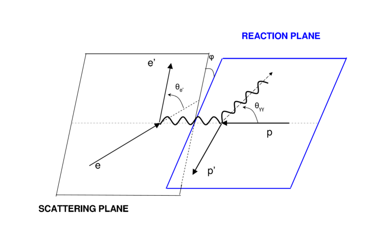
Figure 1: The Virtual Compton Scattering reaction

I.2 Virtual Compton Scattering and the GPs

The generalized polarizabilities can be explored through VCS, which is accessed experimentally by exclusive photon electroproduction as shown in Figure 1. The kinematics are defined by five independent variables, the incoming and final electron energies, the scattered electron angle, and the polar and azimuthal angles of the Compton subprocess in its center-of-mass. Due to electron scattering, one also has the Bethe-Heitler process (BH) where the final photon is emitted by the incoming or outgoing electron. The photon electroproduction amplitude is the coherent sum of the Bethe-Heitler, Born and non-Born contributions as shown in Figure 2. The (BH) and (Born) parts, produced due to bremsstrahlung of the electron or proton, respectively, are well known and are entirely calculable with the nucleon EM form factors as inputs, while the non-Born amplitude contains the dynamical internal structure information in terms of GPs.

The LET (Low energy theorem) [3] provides a path to access these observables analytically. According to the LET, or LEX (Low-energy EXpansion), the amplitude $T^{ep\gamma}$ is expanded in powers of $q^{\prime}_{cm}$. As a result, the (unpolarised) $ep\rightarrow ep\gamma$ cross section at small $q^{\prime}_{cm}$ can be written as:   

$$d^{5}\sigma = d^{5}\sigma^{BH+Born}\ +\ q^{\prime}_{cm}\cdot\phi\cdot\Psi_{0}\ +\ {\cal O}(q^{\prime 2}_{cm})\ \ \$$ (2)

where $\phi$ is a phase-space factor. The notation $d^{5}\sigma$ stands for $d^{5}\sigma/dk^{\prime}_{elab}d\Omega^{\prime}_{elab}d\Omega_{cm}$ where $k^{\prime}_{elab}$ is the scattered electron momentum in the lab frame, $d\Omega^{\prime}_{elab}$ its solid angle in the lab frame and $d\Omega_{\gamma cm}$ the solid angle of the outgoing photon (or proton) in the $p$-$\gamma^{*}$ CM frame. The $\Psi_{0}$ term comes from the interference between the Non-Born and the BH+Born amplitudes at lowest order in $q^{\prime}_{cm}$; it gives the leading polarizability effect in the cross section. The LET approach is valid only below the pion production threshold, i.e. as long as the Non-Born amplitude remains real.

The $\Psi_{0}$ term contains three structure functions $P_{LL}$, $P_{TT}$ and $P_{LT}$:   

$$\Psi_{0} = v_{1}\cdot(P_{LL}-{\displaystyle 1\over\displaystyle\epsilon}P_{TT})\ +\ v_{2}\cdot P_{LT}$$ (3)

where $\epsilon$ is the usual virtual photon polarisation parameter and $v_{1},v_{2}$ are kinematical coefficients depending on $(q_{cm},\epsilon,\theta_{cm},\varphi)$. $\theta_{cm}$ and $\varphi$ are the polar and azimuthal angles of the Compton scattering process in the CM frame of the initial proton and virtual photon (Fig. 1). The full expression of $v_{1},v_{2}$ can be found in ref [3], as well as the expression of the structure functions versus the GPs. For the structure functions one has:   

$$\begin{array}[]{lll}P_{LL}&=&{4M\over\alpha_{em}}\cdot G_{E}^{p}(Q^{2})\cdot\alpha_{E}(Q^{2})\\ \\ P_{TT}&=&[P_{TT~{}spin}]\\ \\ P_{LT}&=&-{2M\over\alpha_{em}}\sqrt{{q_{cm}^{2}\over Q^{2}}}\cdot G_{E}^{p}(Q^{2})\cdot\beta_{M}(Q^{2})+[P_{LT~{}spin}]\end{array}$$ (9)

where $\alpha_{em}$ is the fine structure constant and the terms in brackets are the spin part of the structure functions:

$$\begin{array}[]{lll}P_{TTspin}&=&-3G_{M}^{p}(Q^{2})\,{q_{cm}^{2}\over{\tilde{q}^{0}}}\cdot(P^{(M1,M1)1}(Q^{2})\\ &&-{\sqrt{2}}\,{\tilde{q}^{0}}\cdot P^{(L1,M2)1}(Q^{2})\\ \\ P_{LTspin}&=&{3\over 2}\,{q_{cm}\sqrt{Q^{2}}\over\tilde{q}^{0}}G_{M}^{p}(Q^{2})\cdot P^{(L1,L1)1}(Q^{2})\end{array}$$ (14)

where $\tilde{q}^{0}$ is the CM energy of the virtual photon in the limit $q^{\prime}_{cm}\to 0$. One can note that $P_{LL}$ is proportional to the electric GP, and the scalar part of $P_{LT}$ is proportional to the magnetic GP. Using this LET approach one cannot extract all six dipole GPs separately from an unpolarised experiment since only three independent structure functions appear and can be extracted assuming the validity of the truncation to ${\cal O}(q^{\prime 2}_{cm})$. Furthermore in order to isolate the scalar part in these structure functions a model input is also required.

However, since the sensitivity of the VCS cross sections to the GPs grows with the photon energy it is advantageous to go to higher photon energies. Above the pion threshold the VCS amplitude becomes complex. While $T^{BH}$ and $T^{Born}$ remain real, the amplitude $T^{Non-Born}$ acquires an imaginary part, due to the coupling to the $\pi$N channel. The relatively small effect of GPs below the pion threshold, which is contained in $d\sigma_{Non-Born}$, becomes more important in the region above the pion threshold and up to the $\Delta(1232)$ resonance, where the LET does not hold. In this case a Dispersion Relations (DR) formalism is prerequisite to extract the polarizabilities in the energy region above pion threshold where the observables are generally more sensitive to the GPs.

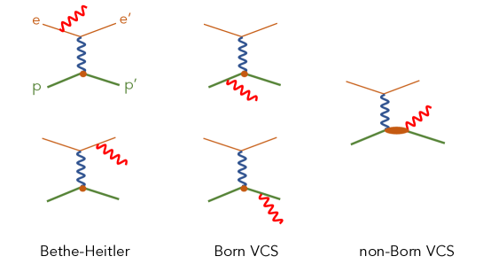
Figure 2: Feynman diagrams of photon electroproduction, illustrating the mechanisms contributing to ep$\rightarrow$ep$\gamma$. The small circles represent the interaction vertex of a virtual photon with a proton considered as a point-like particle, while the ellipse denotes the non-Born VCS amplitude.

The Dispersion Relations (DR) formalism developed by B.Pasquini et al. [8, 9] for RCS and VCS allows the extraction of structure functions and GPs from photon electroproduction experiments. The calculation provides a rigorous treatment of the higher-order terms in the VCS amplitude, up to the $N\pi\pi$ threshold, by including resonances in the $\pi N$ channel. The Compton tensor is parameterised through twelve invariant amplitudes $F_{i}(i=1,12)$. The GPs are expressed in terms of the non-Born part $F_{i}^{NB}$ of these amplitudes at the point $t=-Q^{2},\nu=(s-u)/4M=0$, where $s,t,u$ are the Mandelstam variables of the Compton scattering. All of the $F_{i}^{NB}$ amplitudes, with the exception of two, fulfill unsubtracted dispersion relations. These $s$-channel dispersive integrals are calculated through unitarity. They are limited to the $\pi N$ intermediate states, which are considered to be the dominant contribution for describing VCS up to the $\Delta(1232)$ resonance region. The calculation uses pion photo- and electroproduction multipoles [10] in which both resonant and non-resonant production mechanisms are included. The amplitudes $F_{1}$ and $F_{5}$ have an unconstrained part beyond the $\pi N$ dispersive integral. Such a remainder is also considered for $F_{2}$. For $F_{5}$ this asymptotic contribution is dominated by the t-channel $\pi^{0}$ exchange, and with this input all four spin GPs are fixed. For $F_{1}$ and $F_{2}$, an important feature is that in the limit $(t=-Q^{2},\nu=0)$ their non-Born part is proportional to the GPs $\beta_{M}$ and $(\alpha_{E}+\beta_{M})$, respectively. The remainder of $F_{1,2}^{NB}$ is estimated by an energy-independent function, noted $\Delta\beta$ and $\Delta(\alpha+\beta)$ respectively. This term parameterises the asymptotic contribution and/or dispersive contributions beyond $\pi N$. For the magnetic GP one gets:   

$$\begin{array}[]{lll}\beta_{M}(Q^{2})&=&\beta^{\pi N}(Q^{2})+\Delta\beta\\ \\ \Delta\beta&=&{\displaystyle[\beta^{exp}-\beta^{\pi N}]_{Q^{2}=0}\over\displaystyle(1+Q^{2}/\Lambda^{2}_{\beta})^{2}}\ .\end{array}$$ (18)

The sum $(\alpha_{E}+\beta_{M})$ follows a similar decomposition, and thus the electric GP too:   

$$\begin{array}[]{lll}\alpha_{E}(Q^{2})&=&\alpha^{\pi N}(Q^{2})+\Delta\alpha\\ \\ \Delta\alpha&=&{\displaystyle[\alpha^{exp}-\alpha^{\pi N}]_{Q^{2}=0}\over\displaystyle(1+Q^{2}/\Lambda^{2}_{\alpha})^{2}}\ .\end{array}$$ (22)

The two scalar GPs are not fixed by the model, and their unconstrained part is parametrised by a dipole form, as given by eqs.(18,22). This dipole form is arbitrary while the mass parameters $\Lambda_{\alpha}$ and $\Lambda_{\beta}$ only play the role of intermediate quantities in order to extract VCS observables. In the DR calculation $\Lambda_{\alpha}$ and $\Lambda_{\beta}$ are treated as free parameters, which can furthermore vary with $Q^{2}$. Their value can be adjusted by a fit to the experimental cross section, separately at each $Q^{2}$. Then the calculation is fully constrained and provides all VCS observables, the scalar GPs as well as the structure functions, at this $Q^{2}$.

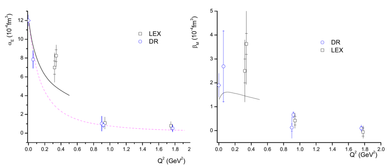
Figure 3: World data from the early experiments [11, 12, 13, 14, 15, 16] on the electric GP $\alpha_{E}$ and the magnetic GP $\beta_{M}$. Open circles correspond GPs extracted through DR while the open boxes through LEX. The solid curve corresponds to HBChPT [21, 22]. The dipole fall off of $\alpha_{E}$ (dashed line) from the DR calculation [8, 9] is able to describe all world data except the MAMI measurements.

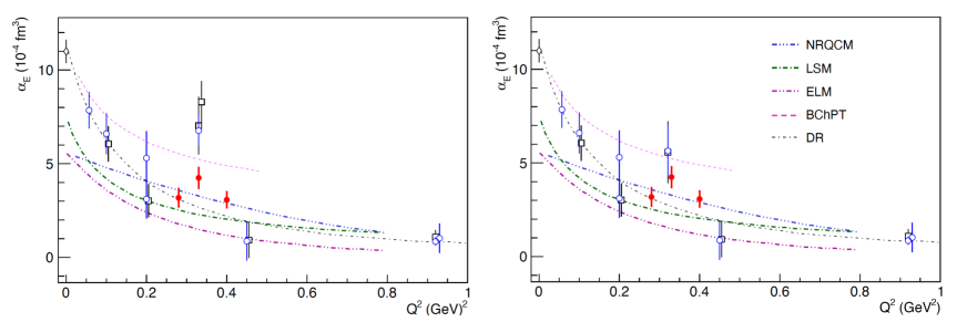
Figure 4: Left panel: The world data for $\alpha_{E}$. The recent results from MAMI [42, 43, 44] are shown as open symbols and those of the JLab VCS-I experiment [2] as filled red circles. The results from the early experiments (already referenced in Fig. 3) are also shown with open symbols. Right panel: Same as in the left panel, but with the re-analysis of the MAMI data at $Q^{2}=0.33~{}GeV^{2}$ [49, 50]. The theoretical predictions of [25, 26, 27, 28, 29, 30, 31, 45] are also shown.

I.3 The experimental and theoretical landscape of the GPs

A group of early VCS experiments, that was performed at MAMI [11, 12], JLab [13, 14] and Bates [15, 16] nearly two decades ago, shaped a first understanding of the proton electric and magnetic GPs. They involved measurements below and above the pion threshold, that were analyzed both within the LEX and the DR approach. The measurements illustrated the good agreement in the extraction of the GPs following the two different methods, as well as the consistency in the GPs extraction from measurements that were conducted below and above the pion threshold, and up to the first resonance region [13, 14]. The measurements have furthermore highlighted the enhanced sensitivity to the GPs as one measures above the pion production threshold. These early measurements, as illustrated in Fig. 3, presented experimental evidence that contradict the naive Ansatz of a single-dipole fall-off for $\alpha_{E}(Q^{2})$, pointing out to an enhancement at low $Q^{2}$ evidenced by the MAMI measurements [11, 12]. Here, two independent experiments [11, 12] were able to confirm this unexpected structure for $\alpha_{E}$. For the magnetic GP, a first experimental description with relatively large uncertainties was provided by these experiments, highlighting the challenges in extracting the magnetic polarizability signal.

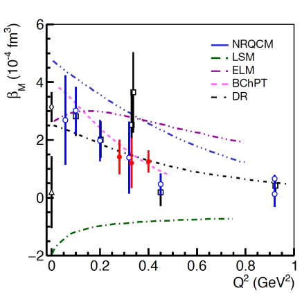
Figure 5: The magnetic generalized polarizability. The references are the same as in Fig. 4.

A recent generation of experiments provided an improved and more extended study of the proton GPs. The experiments were conducted at MAMI [42, 43, 44] and at JLab [2] and their results are shown in Figs. 4 and 5. The reported measurements provided evidence of a local structure (e.g. an enhancement or plateau) of $\alpha_{E}$, at the same $Q^{2}$ as previously reported in [11, 12], but with a smaller magnitude than what was originally suggested. In parallel, the data analysis of the early MAMI experiment [11, 12] was revisited, accounting for refinements in the analysis procedure that were developed recently and were considered in the analysis of the latest MAMI measurements [42, 43]. The re-analysis of these data (as presented in [49, 50], currently unpublished) reduces slightly the extracted value for $\alpha_{E}$ and brings it in agreement with the JLab VCS-I results [2], as shown in Fig. 4 (right panel). A local non-trivial structure in $\alpha_{E}$, as suggested by both the JLab and the MAMI measurements, presents a striking contradiction to our theoretical understanding. The mesonic cloud effects may present a potential candidate for the processes involved in this effect, but the presence of a dynamical mechanism that is not accounted for in the theory can’t be excluded. The signature of this effect has so far been explored [2] with phenomenological fits as well as with methods that do not assume any direct underlying functional form [46], as shown in Fig. 7(a) and Fig. 7(c) respectively. In light of the recent results, the need for new experimental measurements becomes evident. They will allow to increase the statistical significance in the observation of the local enhancement in $\alpha_{E}$, that deviates from the theoretically predicted monotonic $Q^{2}$ dependence, currently at the 3$\sigma$ level. The shape and the dynamical signature of this structure needs to be clearly mapped with high precision measurements, so that it can serve as an input for the theory towards explaining the effect. The motivation for new measurements extends further, to the study of the magnetic GP. Here, the magnitude of the signal is smaller compared to $\alpha_{E}$, as shown in Fig. 5. This renders the $\beta_{M}$ more sensitive to the experimental errors and challenges our access in the physics of interest. Reported discrepancies [47, 48] in the measurement of the static ($Q^{2}=0$) magnetic polarizability, as shown in Fig. 5, highlight the need to improve these measurements, particularly at low momentum transfers. Recent experiments have illustrated our ability to measure $\beta_{M}$ with high precision. Extending these measurements will provide a key to understand the processes manifesting in the interplay between diamagnetism and paramagnetism in the proton, and represents an excellent opportunity to gain a deep insight to the structure and the dynamics of the nucleon.

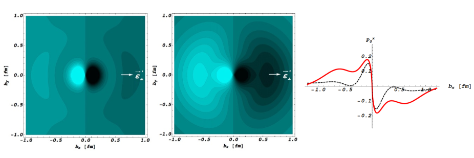
Figure 6: Figure from [34]. Induced polarization, $P_{0}^{x}$, in a proton of definite light-cone helicity, when submitted to an e.m. field with photon polarization along the $x$-axis, as indicated. Left (center) panel is for GP I (GP II), see text. The light (dark) regions correspond to the largest (smallest) values. The right panel compares $P_{0}^{x}$ along $b_{y}=0$ : dotted curve is for GP I; solid curve is for GP II.

In analogy to the relation that connects the proton electric form factor to the proton charge radius, the generalized polarizabilities allow access to the electromagnetic polarizability radii of the proton. The mean square electric polarizability radius of the proton $\langle r^{2}_{\alpha_{E}}\rangle$ is related to the slope of the electric GP at $Q^{2}=0$ by

$$\langle r^{2}_{\alpha_{E}}\rangle=\frac{-6}{\alpha_{E}(0)}\cdot\frac{d}{dQ^{2}}\alpha_{E}(Q^{2}){\bigg{|}}_{Q^{2}=0}.$$ (23)

In a procedure that is equivalent to that for the extraction of the proton charge radius, fits to the world-data [2] of the electric generalized polarizabilities, as shown in Fig. 7(a), lead to a value for the mean square electric polarizability radius $\langle r^{2}_{\alpha_{E}}\rangle=1.36\pm 0.29~{}fm^{2}$. This value is considerably larger compared to the mean square charge radius of the proton, $\langle r^{2}_{E}\rangle\sim 0.7~{}fm^{2}$ (see Fig. 7(b)). The dominant contribution to this effect is expected to arise from the deformation of the mesonic cloud in the proton under the influence of an external EM field. Similarly, the mean square magnetic polarizability radius has been extracted from the magnetic polarizability measurements $\langle r^{2}_{\beta_{M}}\rangle=0.63\pm 0.31~{}fm^{2}$. A new set of measurements for the proton electromagnetic GPs will allow to improve further the precision in the extraction of the proton polarizability radii.

Significant theoretical progress has been achieved in recent years towards our understanding of the generalized polarizabilities. The GPs have been calculated following a variety of approaches, as shown in Fig. 4. A common feature is that none of the theoretical calculations is able to describe a non-trivial structure of $\alpha_{E}$, as they all predict a smooth $Q^{2}$ fall-off. In heavy baryon chiral perturbation theory (HBChPT) the polarizabilities are pure one-loop effects to leading order in the chiral expansion [19], emphasizing the role of the pion cloud; the scalar GPs have been calculated to order $p^{3}$ [20, 21, 22], while the spin GPs have been calculated to order $p^{4}$ [23, 24]. The first nucleon resonance $\Delta(1232)$ is taken into account either by local counterterms (ChPT, [19]) or as an explicit degree of freedom (small scale expansion SSE of [22]). In non-relativistic quark constituent models [3, 25, 26, 27] the GPs involve the summed contribution of all nucleon resonances but do not embody a direct pionic effect. The calculation of the linear-$\sigma$ model [28, 29] involves all fundamental symmetries but does not include the $\Delta$ resonance, while the effective lagrangian model [30] includes resonances and the pion cloud in a more phenomenological way. A calculation of the electric GP was made in the Skyrme model [31]. Recent calculations of the generalized polarizabilities have been performed in baryon chiral perturbation theory [45]. Lattice calculations are for the moment limited to polarizabilities in RCS [32] but significant progress on that front is expected in the near future. Future experimental measurements, such as those presented in this proposal, will provide high-precision benchmark data for these calculations, offering valuable input and guidance to the theory.

The formalism to extract light-front quark charge densities from nucleon form factor data has been extended in recent years to the deformation of the quark charge densities when applying an external electric field  [33, 34]. This in-turn allows for the concept of GPs to be used to describe the spatial deformation of the charge and magnetization densities. The correlation of the GPs to the induced polarization in a proton when submitted to an e.m. field is illustrated in the theoretical calculations shown in Fig. 6, where two parametrizations, GP-I (dipole fall-off) and GP-II (a parametrization of a dipole+gaussian), have been considered for $\alpha_{E}$ [35]. An $\alpha_{E}$ enhancement at intermediate $Q^{2}$, as opposed to a pure dipole fall-off, tends to extend the spatial distribution of the induced polarization to larger transverse distances. An experimental extraction of the induced polarization in the proton from a fit to the world data [2] is shown in Fig. 7(d). Upcoming experiments will allow to improve further the precision of this extraction, offering a detailed spatial representation of the induced polarization in the proton.

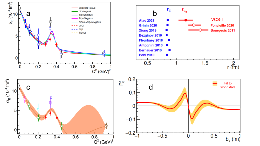
Figure 7: a) Mean square electric polarizability radius fits using combinations of different functional forms. The fits denoted with solid lines were performed over the full $Q^{2}$-range of the world-data. The functional forms denoted with dashed lines were performed in the low-$Q^{2}$ range, namely in $Q^{2}$=[0,0.28] GeV².b) The proton electric polarizability radius $r_{\alpha_{E}}\equiv\sqrt{\langle r^{2}_{\alpha_{E}}\rangle}$ is shown in red. The measurements of the proton charge radius are shown for comparison in blue color. c) The $Q^{2}$-dependence of the electric GP as derived from the experimental measurements using the GPR technique [46], a data-driven method that assumes no direct underlying functional form. d) Induced polarization in the proton when submitted to an EM field as a function of the transverse position with photon polarization along the x axis for $b_{y}=0$. The x-y defines the transverse plane, with the z axis being the direction of the fast moving protons.

II The Experiment

The proposed experiment aims to provide high precision measurements of $\alpha_{E}$ and $\beta_{M}$ in the region of $Q^{2}=0.05~{}(GeV/c)^{2}$ to $Q^{2}=0.50~{}(GeV/c)^{2}$. The proposed measurements will allow to pin down the dynamic signature of the two scalar GPs with a high precision, providing access to the underlying reaction mechanisms in the proton. They will further explore the puzzling structure that has been observed in the electric GP, aiming to identify the shape of this structure that will serve as valuable input to the theory. More specifically, the selection of the proposed kinematics has been done considering recent measurements and findings for the proton GPs, along with the demonstrated potential to improve upon the precision of the world data with measurements at JLab, towards the following goals:

i) Provide high precision measurements combined with a fine mapping as a function of $Q^{2}$, lower and higher in $Q^{2}$ with respect to the kinematics that are of particular interest for $\alpha_{E}$. This is vital, since it will allow to explore the dynamical signature of $\alpha_{E}$ through a set of measurements that are all uniform in regard to their systematic uncertainties. This will in-turn provide further clarity in the study of the suggested structure for the $\alpha_{E}$ and in identifying it’s shape with precision.

ii) Provide measurements within targeted kinematics where the sensitivity to the polarizabilities is appreciably changing. For the particular case of $\alpha_{E}$, complementary measurements at the same $Q^{2}$ will be conducted within kinematics where the suggested structure in the polarizability emerges in an anti-diametric way in the VCS cross section. These measurements will allow to fully de-couple the observation of a non-trivial structure in the polarizability from the influence of experimental uncertainties that are of systematic nature.

iii) Improve significantly the precision in the measurement of the $\beta_{M}$. The world data for $\beta_{M}$ are characterized by relatively large uncertainties and they do not provide sufficient information to decode the interplay of the paramagnetic and diamagnetic mechanisms in the proton, that are particularly profound in the low $Q^{2}$ region. Recent measurements at $Q^{2}=0$ [47, 48] reported discrepancies in the measurements of the magnetic GP. They have added to the world-data tension and have further challenged our understanding of $\beta_{M}$. The results from VCS-I [2] have illustrated that we can improve tremendously upon our knowledge of the magnetic GP through a follow-up series of measurements, as proposed in this work.

II.1 The experimental setup

The experiment will utilize standard Hall C equipment to provide measurements of the Virtual Compton Scattering. A schematic representation of the experimental setup is presented in Fig. 8. The SHMS and HMS spectrometers [38, 39] will be used to detect electrons and protons in coincidence respectively, while the reconstructed missing mass will provide the identification of the photon. An electron beam of $E_{\circ}=1.1$ and $2.2~{}GeV$ with current up to $I=75\mu$A, along with a 10 cm long liquid hydrogen target will be required for this measurement. The GPs will be measured within the range of $Q^{2}=0.05~{}(GeV/c)^{2}$ to $Q^{2}=0.50~{}(GeV/c)^{2}$.

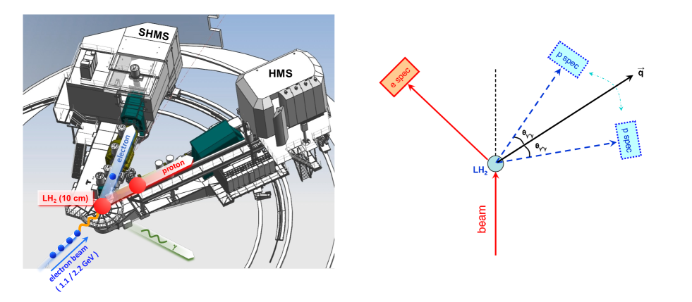
Figure 8: Left: An illustration of the proposed experimental setup in Hall C. Right: Positioning the proton spectrometer symmetrically with respect to the momentum transfer direction allows to measure the azimuthal asymmetry of the VCS cross section, where part of the systematic uncertainties get suppressed. By keeping both magnet settings unchanged between the two asymmetry measurements, the spectrometer momenta can be precisely determined through the cross-calibration of the two reconstructed missing mass spectra.

A beam energy of $E_{\circ}=1.1~{}GeV$ is required only for the lowest $Q^{2}$ setting, at $Q^{2}=0.05~{}(GeV/c)^{2}$. All the other measurements request a beam of $E_{\circ}=2.2~{}GeV$. The value for the beam energy has been chosen so that it can simultaneously accommodate the maximum beam energy of the accelerator in another Hall. Nevertheless, its exact value can be flexibly adjusted as needed, with a minimal impact in the extraction of the GPs. The choice of the kinematic settings has been driven by the sensitivity of the Compton scattering observables to the polarizabilities, in tandem with physical constraints of the experimental setup. The measurements will target kinematics above the pion threshold, that offer enhanced sensitivity to the GPs. They will span a wide range of energies and photon angles, typically above $\theta_{\gamma^{*}\gamma}\approx$ 100^∘ in order to satisfy the physical restrictions in the Hall and to avoid the kinematic range where the BH process dominates the cross section (e.g. see Fig. 9) and suppresses the sensitivity to the GPs. Measurements of the in-plane azimuthal asymmetry of the VCS cross section with respect to the momentum transfer direction will be conducted, for fixed $\theta_{\gamma^{*}\gamma}$ at $\phi_{\gamma^{*}\gamma}=0^{\circ}$ and $\phi_{\gamma^{*}\gamma}=180^{\circ}$   
$A_{(\phi_{\gamma^{*}\gamma}=0,\pi)}=\frac{\sigma_{\phi_{\gamma^{*}\gamma}=0}-\sigma_{\phi_{\gamma^{*}\gamma}=180}}{\sigma_{\phi_{\gamma^{*}\gamma}=0}+\sigma_{\phi_{\gamma^{*}\gamma}=180}}$   
One benefit emerging from the asymmetry measurements is that part of the systematic uncertainties are suppressed in the ratio, and thus the sensitivity in the extraction of the polarizabilities is enhanced. Furthermore, the asymmetry measurements allow to precisely determine the true momentum settings of the two spectrometers based on the cross-calibration of the missing mass, since the momentum and position of the electron spectrometer remain the same between the two settings while the momentum setting for the proton spectrometer also remains unchanged. This allows to correct for small deviations between the set and the true spectrometer momentum settings and offers a tighter control of the systematic uncertainties.

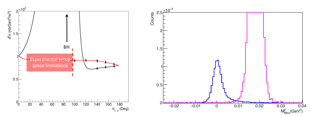
Figure 9: Left panel: Projected cross sections at $Q^{2}=0.35~{}(GeV/c)^{2}$. The black and red curves correspond to cross sections at $\phi_{\gamma^{*}\gamma}=0^{\circ}$ and $180^{\circ}$. The constraints imposed by the BH and by the space limitations of the experimental setup are marked in the figure. Right panel: The reconstructed missing mass spectrum offers a clean separation between the undetected photons and the pions.

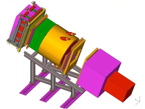
Figure 10: The SHMS detector stack.

Kinematic	Kinematic	HMS singles rates
Group	Setting	(kHz)
	Kin I	43
	Kin II	53
GI	Kin IIIa	119
	Kin IIIb	65
	Kin IVa	128
	Kin IVb	80
	Kin I	159
	Kin IIa	21
GII	Kin IIb	155
	Kin IIIa	28
	Kin IIIb	122
	Kin IVa	42
	Kin IVb	82
	Kin I	347
	Kin IIa	27
GIII	Kin IIb	330
	Kin IIIa	47
	Kin IIIb	214
	Kin IVa	77
	Kin IVb	129
	Kin I	476
	Kin II	497
GIV	Kin IIIa	453
	Kin IIIb	64
	Kin IVa	313
	Kin IVb	89
	Kin Va	212
	Kin Vb	127
	Kin I	483
	Kin II	502
GV	Kin IIIa	444
	Kin IIIb	51
	Kin IVa	295
	Kin IVb	72
	Kin Va	192
	Kin Vb	108
	Kin I	591
	Kin IIa	349
GVI	Kin IIb	33
	Kin IIIa	527
	Kin IIIb	49

Table 2: The combined proton and pion singles rates for the HMS spectrometer. The parameters of the kinematic settings are given in Table 3.

The trigger will be a coincidence between the electrons in the SHMS and the protons in the HMS. The HMS will detect protons using the standard detector package. The protons can be identified by coincidence time-of-flight (TOF). The coincidence time difference between the two spectrometers will vary from 45 ns to 105 ns as the proton momentum varies from 993 to 494 MeV/c. We plan to run with the SHMS trigger window with width of 60ns and the HMS trigger window width of 20ns. An aerogel detector will not be necessary in the HMS detector stack.

The combined proton and pion singles rates have been kept at the level of $\sim 500~{}kHz$ or lower to allow a reliable tracking efficiency calculation. The total singles rates are presented in Table 2.

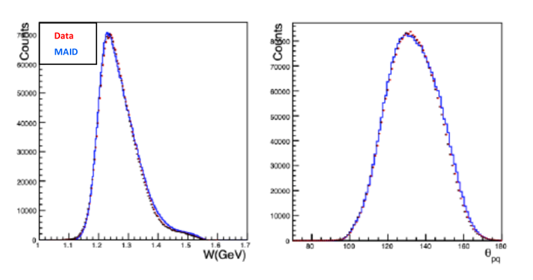
Figure 11: Measurement of the $p(e,e^{\prime}p)\pi^{\circ}$ during the VCS-I experiment. The data (red) are compared to the simulation (blue) weighted with the MAID cross section.

Time will be needed for calibrations that will involve luminosity scans, target boiling, tracking efficiency, electronic deadtime and spectrometer optics. The targets for these studies will be a 10-cm long liquid hydrogen, 10-cm aluminum dummy and optics foil targets. For the elasic $ep$ coincidence measurements, the HMS will be at angles of 50^∘ to 63^∘ and at momentum between 495 to 994 MeV/c while the SHMS will be at angles of 19^∘ to 33^∘ and at momentum between 924 to 1797 MeV/c. Conservatively, one day has been set aside for this in the run plan, but if other experiments are running the time would be shared with these experiments. Two additional days of dummy-runs will also be required throughout the experiment.

The spectrometer acceptance will allow to measure the pion electroproduction reaction simultaneously with the VCS. The two reaction channels will be cleanly separated through the reconstructed missing mass spectrum. The cross section for $p(e,e^{\prime}p)\pi^{\circ}$ is very well known in this region and these measurements will serve as a real-time normalization cross-check during the measurement of the VCS cross section. Fig. 11 shows the measurement of the $p(e,e^{\prime}p)\pi^{\circ}$ during the VCS-I experiment that was conducted using the same experimental setup as the one proposed here. These measurements illustrate the excellent understanding of the spectrometer acceptance in the experiment simulation.

II.2 Kinematic settings and beam time request

The kinematic settings are summarized in Table 3. Monte-Carlo studies have been performed (see Fig. 12) for all of the proposed kinematics using SIMC [40]. The code includes the effects of offsets and finite resolutions while a physics model is averaged over the finite acceptances of the experimental apparatus. The reconstructed missing mass spectrum is presented in Fig. 9. For the calculation of the count rates and the beam time request the Dispersion Relations calculation [8] developed by B. Pasquini was used and folded over the experimental acceptance. The model has been proven very successful both in the calculation of the VCS cross sections above the pion threshold and in the extraction of the GPs [11, 12, 13, 14, 41]. The beam time request per setting is summarized at the last column of Table 3. The accidental rates have been studied for all the kinematical settings. The beam current will vary per setting, to a maximum of I=75 $\mu$A, in order to keep the singles rates within the operational range for both spectrometers. The HMS singles rates will range between approximately 20 kHz and 500 kHz, depending on the setting. The SHMS singles rates will range from 200 kHz to 500 kHz. The coincidence signal to noise (S/N) ratio will range from $\approx$ 7 to 0.3 and for a wide missing mass cut of $\sim 100~{}MeV$; a more tight missing mass applied during the analysis will be able to further improve the S/N ratio. Calibration data will be taken for normalization studies, while these studies will be further complemented by the simultaneous measurement of the $p(e,e^{\prime}p)\pi^{\circ}$ reaction during the VCS measurements, as commented in the previous section.

Kinematic	Kinematic	$\theta_{\gamma^{*}\gamma}^{\circ}$	$\theta_{e}^{\circ}$	$P^{{}^{\prime}}_{e}(MeV/c)$	$\theta_{p}^{\circ}$	$P^{{}^{\prime}}_{p}(MeV/c)$	$I~{}(\mu A)$	beam time
Group	Setting							(days)
	Kin I	$110$	$14.3$	$736.3$	$54.45$	$493.93$	15	1.00
	Kin II	$133$	$14.3$	$736.3$	$44.93$	$556.10$	15	1.00
GI	Kin IIIa	$147$	$14.3$	$736.3$	$11.26$	$583.05$	15	1.00
	Kin IIIb	$147$	$14.3$	$736.3$	$39.06$	$583.05$	15	1.00
	Kin IVa	$160$	$14.3$	$736.3$	$16.73$	$599.95$	15	1.00
	Kin IVb	$160$	$14.3$	$736.3$	$33.59$	$599.95$	15	1.00
	Kin I	$115$	$11.22$	$1783.0$	$15.33$	$615.69$	10	1.50
GII	Kin IIa	$125$	$11.22$	$1783.0$	$56.54$	$647.85$	10	2.50
	Kin IIb	$125$	$11.22$	$1783.0$	$18.60$	$647.85$	10	1.50
	Kin IIIa	$145$	$11.22$	$1783.0$	$49.77$	$697.99$	10	1.50
	Kin IIIb	$145$	$11.22$	$1783.0$	$25.37$	$697.99$	10	1.00
	Kin IVa	$165$	$11.22$	$1783.0$	$42.82$	$726.87$	10	1.00
	Kin IVb	$165$	$11.22$	$1783.0$	$32.32$	$726.87$	10	1.00
	Kin I	$115$	$14.73$	$1729.7$	$20.58$	$706.89$	30	1.75
GIII	Kin IIa	$130$	$14.73$	$1729.7$	$54.89$	$758.24$	30	2.00
	Kin IIb	$130$	$14.73$	$1729.7$	$24.78$	$758.24$	30	1.75
	Kin IIIa	$150$	$14.73$	$1729.7$	$48.99$	$808.24$	30	1.75
	Kin IIIb	$150$	$14.73$	$1729.7$	$30.68$	$808.24$	30	1.75
	Kin IVa	$170$	$14.73$	$1729.7$	$42.90$	$834.12$	30	1.00
	Kin IVb	$170$	$14.73$	$1729.7$	$36.76$	$834.12$	30	1.00
	Kin I	$100$	$16.32$	$1749.3$	$23.83$	$664.52$	35	1.75
GIV	Kin II	$120$	$16.32$	$1749.3$	$28.01$	$738.39$	50	1.25
	Kin IIIa	$140$	$16.32$	$1749.3$	$32.84$	$795.37$	70	1.00
	Kin IIIb	$140$	$16.32$	$1749.3$	$53.80$	$795.37$	70	2.00
	Kin IVa	$155$	$16.32$	$1749.3$	$36.69$	$824.46$	70	1.50
	Kin IVb	$155$	$16.32$	$1749.3$	$49.95$	$824.46$	70	2.50
	Kin Va	$170$	$16.32$	$1749.3$	$40.66$	$840.48$	70	1.00
	Kin Vb	$170$	$16.32$	$1749.3$	$45.99$	$840.48$	70	1.00
	Kin I	$100$	$17.72$	$1676.41$	$19.75$	$723.69$	35	2.00
	Kin II	$120$	$17.72$	$1676.41$	$24.25$	$808.93$	50	1.50
	Kin IIIa	$140$	$17.72$	$1676.41$	$29.34$	$874.74$	70	1.50
GV	Kin IIIb	$140$	$17.72$	$1676.41$	$51.12$	$874.74$	70	2.00
	Kin IVa	$155$	$17.72$	$1676.41$	$33.36$	$908.37$	70	2.00
	Kin IVb	$155$	$17.72$	$1676.41$	$47.10$	$908.37$	70	2.00
	Kin Va	$170$	$17.72$	$1676.41$	$37.47$	$926.91$	70	1.00
	Kin Vb	$170$	$17.72$	$1676.41$	$42.99$	$926.91$	70	1.00
	Kin I	$120$	$20.45$	$1623.1$	$25.31$	$886.59$	75	1.00
GVI	Kin IIa	$140$	$20.45$	$1623.1$	$29.91$	$956.82$	75	1.00
	Kin IIb	$140$	$20.45$	$1623.1$	$49.81$	$956.82$	75	1.50
	Kin IIIa	$155$	$20.45$	$1623.1$	$33.58$	$992.83$	75	1.50
	Kin IIIb	$155$	$20.45$	$1623.1$	$46.14$	$992.83$	75	2.00

Table 3: The kinematic settings of the proposed experiment. A 1100 MeV beam is required for the kinematic group GI (namely for 6 days of beamtime). All other kinematic groups (53 days of beamtime) will require a 2200 MeV beam.

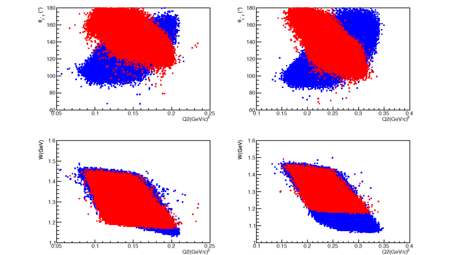
Figure 12: (Left $Q^{2}=0.15~{}GeV^{2}$ and Right $Q^{2}=0.25~{}GeV^{2}$) Correlation of the phase space variables for a pair of $\phi_{\gamma^{*}\gamma}=0^{\circ}$, $180^{\circ}$ measurements, with the two different colors corresponding to $\phi_{\gamma^{*}\gamma}=0^{\circ}$ and $180^{\circ}$ respectively. Left (top and bottom) and right (top and bottom) correspond to a pair of settings from kinematic groups GII and GIII, respectively.

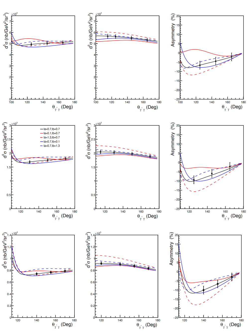
Figure 13: From left to right: cross sections at $\phi_{\gamma^{*}\gamma}=0^{\circ}$ (left) and $180^{\circ}$ (center) and asymmetries (right). Top panels correspond to $Q^{2}=0.15~{}(GeV/c)^{2}$, middle panels to $Q^{2}=0.25~{}(GeV/c)^{2}$ and bottom panels to $Q^{2}=0.35~{}(GeV/c)^{2}$.

The proposed measurements will allow the extraction of the GPs at $Q^{2}=0.05~{}(GeV/c)^{2}$, $Q^{2}=0.15~{}(GeV/c)^{2}$, $Q^{2}=0.25~{}(GeV/c)^{2}$, $Q^{2}=0.31~{}(GeV/c)^{2}$, $Q^{2}=0.35~{}(GeV/c)^{2}$, $0.45~{}(GeV/c)^{2}$, and $0.50~{}(GeV/c)^{2}$. All the settings will require a $E_{\circ}=2.2~{}GeV$ beam, with the exception of the $Q^{2}=0.05~{}(GeV/c)^{2}$ kinematics that will require a beam energy $E_{\circ}=1.1~{}GeV$ The phase space coverage for one pair of asymmetry settings is presented in Fig. 12. With the requested beam time, the cross sections will be measured with a statistical uncertainty ranging from $\pm 1\%$ to $\pm 2\%$, depending on the kinematics. The systematic uncertainties will be the dominant factor, ranging at $\approx\pm 4\%$. The uncertainty of the beam energy and of the scattering angle will introduce a systematic uncertainty to the cross section $\approx\pm 2\%$, varying slightly based on the kinematics. Other sources of systematic uncertainties involve the target density, target length, beam charge, proton absorption, dead-time, and target cell background; each one of these contributes $\pm 0.5\%$ or less to the uncertainty. The correction for contamination of pions under the photon peak will contribute also at a similar level of $\approx\pm 0.5\%$. The uncertainty due to the radiative corrections will be $\pm 1.5\%$. For the tracking efficiencies, we estimate $\pm 0.5\%$ (SHMS) and $\pm 1\%$ (HMS), based on our recent experience from the analysis of the VCS-I experiment. An uncertainty in the determination of the coincidence acceptance is conservatively accounted for at the $\pm 1.5\%$. For the measured asymmetries, the systematic uncertainties are still larger compared to the statistical ones, but not as dominant as in the case of the cross sections. Here, they are expected to be $\approx 1\%$ in absolute asymmetry magnitude. Other considerations that will contribute towards a better control of calibrations and of systematic uncertainties involve the fact that, with the exception of the first $Q^{2}$ setting, the beam energy will remain the same, while the electron spectrometer position and momentum will stay fixed within groups of kinematics.

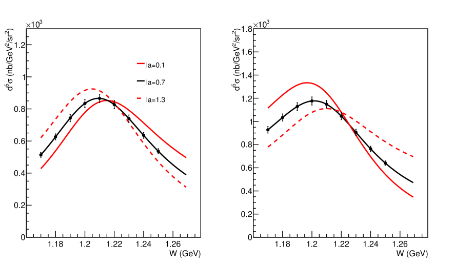
Figure 14: The W-dependence of the cross section at $Q^{2}=0.35~{}(GeV/c)^{2}$ and $\theta_{\gamma^{*}\gamma}=140^{\circ}$, for $\phi_{\gamma^{*}\gamma}=0^{\circ}$ (left) and $180^{\circ}$ (right). The red (solid / dashed) curves illustrate the sensitivity of the VCS cross section to $\alpha_{E}$.

The extraction of the Generalized polarizabilities will be performed in a straightforward way through a fit to the measured cross sections and asymmetries, as was done in previous measurements [13, 14, 44, 42, 43, 2]. The mass scale parameters $\Lambda_{\alpha}$ and $\Lambda_{\beta}$ will be fitted by a $\chi^{2}$ minimization which compares the DR cross sections and asymmetries to the measured ones, and the two scalar GPs will be determined. The systematic uncertainties will play the leading role in the uncertainties of the extracted electric and the magnetic GPs. Another source of uncertainty involves the proton elastic and transition form factors, that enter in the extraction as an input and that are naturally not known with an infinite precision. Here, various parametrizations have been considered and their impact to the extraction of the scalar GPs has been quantified. This effect is comparable to the level of the statistical uncertainties.

In Fig. 13, projected cross sections and asymmetries are presented for three different $Q^{2}$ kinematics and for a fixed $W$ bin. The sensitivity to the electric (and magnetic) generalized polarizability is illustrated through the red (and blue) curves, that correspond to different values for the mass scale parameters $\Lambda_{\alpha}$ (and $\Lambda_{\beta}$, respectively). Improving upon the measurements of the VCS-I experiment, the proposed kinematics extend our physics reach in a targeted way within a region where the sensitivity to the polarizabilities is appreciably changing. In particular for the case of $\alpha_{E}$, the measurements will be conducted within kinematics where the suggested structure (or enhancement) in the polarizability emerges in an anti-diametric way in the VCS cross section. As illustrated in Fig. 14, the VCS cross section sensitivity to the $\alpha_{E}$ undergoes a crossing-point and reverses for the two wings of the resonance. Such targeted measurements will allow to largely de-couple the observation of a non-trivial structure in the polarizability from the influence of experimental uncertainties of systematic nature.

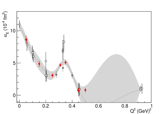
Figure 15: The projected measurements for $\alpha_{E}$ (red circles). The data points are projected along the extraction of the data-driven GPR method, as shown in Fig. 7(c). The world data are shown as black points (the VCS-I results are shown with filled gray circles).

The projected measurements for $\alpha_{E}$ and $\beta_{M}$ are presented in Fig. 15 and Fig. 16, respectively. The experiment will provide high precision measurements combined with a fine mapping as a function of $Q^{2}$, lower and higher in $Q^{2}$ with respect to the kinematics that are of particular interest for $\alpha_{E}$. They will allow to determine the dynamical signature of $\alpha_{E}$ through a set of measurements that are of unprecedented precision and that are all consistent in regard to their systematic uncertainties. The measurements will improve significantly the precision in the extraction of the $\beta_{M}$, providing sufficient information to study the interplay of the paramagnetic and diamagnetic mechanisms in the proton, that is particularly dominant in the low $Q^{2}$ region. The measured GPs will allow to extract with high precision the induced polarization and the electric polarizability radius of the proton. The proposed measurements will contribute significantly to our understanding of the nucleon structure by providing stringent tests and guidance to the theory calculations and high-precision benchmark-data for the upcoming Lattice QCD calculations for the proton GPs, that are expected in the near future.

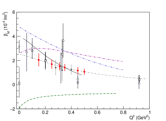
Figure 16: The projected measurements for $\beta_{M}$ (red circles). Similarly to Fig. 15, the world data are shown with black symbols. The theoretical model curves are the same as already referenced in Figs. 4 and 5.

III Summary

We propose to conduct a measurement of the Virtual Compton Scattering reaction in Hall C, using the HMS and SHMS spectrometers, aiming to extract the two scalar Generalized Polarizabilities of the proton in the region of $Q^{2}=0.05~{}(GeV/c)^{2}$ to $Q^{2}=0.50~{}(GeV/c)^{2}$. The experiment will take advantage of the unique capabilities of Hall C, namely the high resolution of the spectrometers along with the ability to position them in small angles. In tandem with an extensive measurement of the kinematic phase space, the experiment will pin down the dynamic signature of $\alpha_{E}$ and $\beta_{M}$ with a high precision and a fine mapping as a function of $Q^{2}$. The proposed measurements will greatly advance our current knowledge of both $\alpha_{E}$ and $\beta_{M}$, which are fundamental quantities of the nucleon that are particularly sensitive to the interplay of the quark and pion degrees of freedom, and will contribute significantly to our understanding of the nucleon dynamics. We request a $E_{\circ}=1.1~{}GeV$ and $2.2~{}GeV$ beam at I=75 $\mu$A, a 10 cm liquid hydrogen target and a total of 59 days of beam on target for the proposed experiment: for these 59 days of beamtime, the 53 days will require a beam energy of $E_{\circ}=2.2~{}GeV$ and the 6 days will require $E_{\circ}=1.1~{}GeV$. Three additional days are requested for optics, dummy, and calibration measurements.

References

- [1] H. Fonvieille, B. Pasquini, N. Sparveris, Prog. Part. Nucl. Phys. 113, 103754 (2020)
- [2] R. Li, et al., Nature 611, 265 (2022)
- [3] P.A.M. Guichon, G.Q. Liu and A.W. Thomas, Nucl. Phys. A 591 (1995) 606.
- [4] D. Drechsel, G. Knochlein, A.Y. Korchin, A. Metz, S. Scherer, Phys. Rev. C 57, 941 (1998)
- [5] D. Drechsel, G. Knochlein, A.Y. Korchin, A. Metz, S. Scherer, Phys. Rev. C 58, 1751 (1998)
- [6] V. Olmos de Leon, et al., Eur. Phys. J. A10 (2001) 207
- [7] Pasquini, B. and Vanderhaeghen, M. Dispersion Theory in Electromagnetic Interactions Annu. Rev. Nucl. Part. Sci. 68, 75-103 (2018).
- [8] B. Pasquini, M. Gorchtein, D. Drechsel, A. Metz, M. Vanderhaeghen, Eur. Phys. J. A11 (2001) 185-208.
- [9] D. Drechsel, B. Pasquini, M. Vanderhaeghen, Phys. Rept. 378 (2003) 99-205.
- [10] D. Drechsel, O. Hanstein, S.S. Kamalov, L. Tiator, Nucl. Phys. A 645, 145 (1999)
- [11] J. Roche, et al., Phys. Rev. Lett. 85 (2000) 708-711.
- [12] P. Janssens, et al., Eur. Phys. J. A37 (2008) 1-8
- [13] G. Laveissiere, et al., Phys. Rev. Lett. 93 (2004) 122001
- [14] H. Fonvieille, et al., Phys. Rev. C86 (2012) 015210
- [15] P. Bourgeois, et al., Phys. Rev. Lett. 97 (2006) 212001
- [16] P. Bourgeois, et al., Phys. Rev. C 84 (2011) 035206
- [17] MAMI experiment A1/1-09, H. Fonvieille et al, A study of the -dependence of the structure functions and and the generalized polarizabilities and in Virtual Compton Scattering at MAMI.
- [18] MAMI experiment A1/3-12, N. Sparveris et al, Study of the nucleon structure by Virtual Compton Scattering measurements at the resonance.
- [19] V. Bernard, N. Kaiser, A. Schmidt, U.G. Meissner, Phys. Lett. B 319, 269 (1993) and references therein
- [20] T. R. Hemmert, B. R. Holstein, G. Knochlein, S. Scherer, Phys. Rev. D55 (1997) 2630-2643.
- [21] T. R. Hemmert, B. R. Holstein, G. Knochlein, S. Scherer, Phys. Rev. Lett. 79 (1997) 22-25.
- [22] T. R. Hemmert, B. R. Holstein, G. Knochlein, D. Drechsel, Phys. Rev. D62 (2000) 014013.
- [23] C. W. Kao, M. Vanderhaeghen, Phys. Rev. Lett. 89 (2002) 272002.
- [24] C.-W. Kao, B. Pasquini, M. Vanderhaeghen, Phys. Rev. D70 (2004) 114004.
- [25] G. Q. Liu, A. W. Thomas, P. A. M. Guichon, Austral. J. Phys. 49 (1996) 905-918.
- [26] B. Pasquini, S. Scherer, D. Drechsel, Phys. Rev. C63 (2001) 025205.
- [27] B. Pasquini, G. Salme, Phys. Rev. C57 (1998) 2589.
- [28] A. Metz, D. Drechsel, Z. Phys. A356 (1996) 351-357.
- [29] A. Metz, D. Drechsel, Z. Phys. A359 (1997) 165-172.
- [30] M. Vanderhaeghen, Phys. Lett. B368 (1996) 13-19.
- [31] M. Kim, D.-P. Min (1997) [hep-ph/9704381]
- [32] W. Detmold, B. Tiburzi, A. Walker-Loud, Phys. Rev. D 81, 054502(2010)
- [33] A.I. Lvov, S. Scherer, B. Pasquini, C. Unkmeir, D. Drechsel, Phys. Rev. C 64, 015203 (2001)
- [34] M. Gorchtein, C. Lorc´e, B. Pasquini, M. Vanderhaeghen, Phys.Rev. Lett. 104, 112001 (2010)
- [35] B. Pasquini, D. Drechsel, and M. Vanderhaeghen, Eur. Phys. J. Special Topics 198, 269285 (2011)
- [36] H. Fonvieille, Talk at “New Vistas in Low-Energy Precision Physics (LEPP)”, Mainz, April 2016; https://indico.mitp.uni-mainz.de/event/66/session/3/contribution/25/material/slides/1.pdf
- [37] N.D.’Hose, Eur. Phys. J. A28, S01 (2006) 117-127
- [38] https://www.jlab.org/Hall-C/upgrade/
- [39] https://www.jlab.org/Hall-C/equipment/HMS.html
- [40] https://hallcweb.jlab.org/wiki/index.php/Monte_Carlo
- [41] N. Sparveris et al, Phys. Rev. C 78, 025209 (2008)
- [42] J. Bericic, et al., Phys. Rev. Lett. 123 (2019) 192302
- [43] H. Fonvieille, et al., Phys. Rev. C 103 (2021) 025205
- [44] A. Blomberg, et al., Eur. Phys. J A 55, 182 (2019)
- [45] V. Lensky, V. Pascalutsa, and M. Vanderhaeghen, Eur. Phys. J. C77, 119 (2017).
- [46] Rasmussen, C. E., and Williams, C. K. I. Gaussian Processes for Machine Learning the MIT Press, Cambridge Massachusetts, 2006, ISBN 026218253X, ©2006 Massachusetts Institute of Technology
- [47] X. Li, et al., Phys. Rev. Lett. 128 (2022) 132502
- [48] E. Mornacchi e, et al., Phys. Rev. Lett. 128 (2022) 132503
- [49] Fonvieille, H., Conference talk, EINN 2017, Cyprus, (http://2017.einnconference.org/wp-content/uploads/2017/11/EINN-2017-Final-Programme.pdf)
- [50] H. Fonvieille, Lecture, Virtual Compton Scattering, SFB School 2017, Boppard (https://indico.mitp.uni-mainz.de/event/89/)