gSASRec: Reducing Overconfidence in Sequential Recommendation Trained with Negative Sampling

Abstract.

A large catalogue size is one of the central challenges in training recommendation models: a large number of items makes them memory and computationally inefficient to compute scores for all items during training, forcing these models to deploy negative sampling. However, negative sampling increases the proportion of positive interactions in the training data, and therefore models trained with negative sampling tend to overestimate the probabilities of positive interactions – a phenomenon we call overconfidence. While the absolute values of the predicted scores/probabilities are not important for the ranking of retrieved recommendations, overconfident models may fail to estimate nuanced differences in the top-ranked items, resulting in degraded performance. In this paper, we show that overconfidence explains why the popular SASRec model underperforms when compared to BERT4Rec. This is contrary to the BERT4Rec authors’ explanation that the difference in performance is due to the bi-directional attention mechanism. To mitigate overconfidence, we propose a novel Generalised Binary Cross-Entropy Loss function (gBCE) and theoretically prove that it can mitigate overconfidence. We further propose the gSASRec model, an improvement over SASRec that deploys an increased number of negatives and the gBCE loss. We show through detailed experiments on three datasets that gSASRec does not exhibit the overconfidence problem. As a result, gSASRec can outperform BERT4Rec (e.g. +9.47% NDCG on the MovieLens-1M dataset), while requiring less training time (e.g. -73% training time on MovieLens-1M). Moreover, in contrast to BERT4Rec, gSASRec is suitable for large datasets that contain more than 1 million items.

1. Introduction

Sequential Recommender Systems is a class of recommender systems that take into account the order of user-item interactions and aim to predict the next item in a sequence. Taking order into account is important in many recommendation scenarios – for example, if a user just bought a mobile phone, then the next purchase is likely to be an accessory for this phone, and hence it makes sense to recommend such accessories to the user. Recently, models based on architectures developed for natural language modelling (particularly using Transformers (Vaswani et al., 2017)) have achieved state-of-the-art performance in sequential recommendation (Kang and McAuley, 2018; Sun et al., 2019; Qiu et al., 2022; Petrov and Macdonald, 2022b, a, 2023a). The success of these language model architectures for sequential recommendation is explained by the similarities between modelling sequences of words in texts and modelling sequences of user-item interactions. However, a direct adaptation of language model architectures for sequential recommendation can be problematic because the number of items in the system catalogue can be much larger than the corresponding vocabulary size of the language models. For example, YouTube has a catalogue of more than 800 million videos. In practice, a direct adaptation of language models with catalogue sizes exceeding 1 million items is computationally prohibitive (Petrov and Macdonald, 2022a, 2023a). Indeed, compared with traditional matrix factorisation models that compute one score distribution per user, sequential recommendation models are usually trained to predict scores for each position in the sequence, meaning that the model has to generate $S*N$ scores per sequence, where $S$ is the sequence length, and $N$ is the size of the catalogue. For example, to train a sequential recommendation model with 64 sequences of 200 items per batch, having 1M items, would require  51GB GPU memory without accounting for the training gradients. Factoring in the gradients and model weights increase this to more than 100Gb, thereby exceeding consumer-grade GPU capacities.

A typical solution for this training problem is negative sampling: the models are trained on all positive interactions (the user-item interactions present in the training set) but only sample a very small fraction of negative interactions (all other possible but unseen user-item interactions). Negative sampling is known to be one of the central challenges (Rendle, 2022) in training recommender systems: it increases the proportion of positive samples in the training data distribution, and therefore models learn to overestimate the probabilities of future user-item interactions. We describe this phenomenon as overconfidence. While the magnitude of retrieval scores is typically non-important for the ranking of items, overconfidence is problematic because models frequently fail to focus on nuanced variations in the highly-scored items and focus on distinguishing top vs. bottom items instead. Another problem caused by overconfidence is more specific to models trained with the popular Binary Cross-Entropy loss: if an item $i$ with high predicted probability $p_{i}$ is sampled as a negative, $\log(1-p_{i})$ calculated by the loss function tends to $-$infinity, causing numerical overflows and unstable training. Overall, we argue that overconfidence hinders model effectiveness and makes model training hard.

Although overconfidence is a general problem applicable to all recommender systems trained with negative sampling, in this paper, we focus specifically on sequential recommender systems, for which negative sampling is specifically important, due to the large GPU memory requirement discussed above. Indeed, as we show in this paper, the use of negative sampling leads to overconfidence in the popular SASRec (Kang and McAuley, 2018) sequential recommendation model. Existing solutions that can address overconfidence induced by negative sampling in recommender systems (e.g. (Rendle and Freudenthaler, 2014; Yuan et al., 2016)) are hard to adapt to deep learning-based sequential recommender models (see also Section 2.1). Hence, the overconfidence issue present in negatively-sampled sequential recommendation models remains largely unsolved. Indeed, the state-of-the-art BERT4Rec (Sun et al., 2019) model does not use negative sampling and, therefore, cannot be applied to datasets with large catalogues.

Hence, to address the overconfidence issue in the sequential recommendation, we introduce a novel Generalised Binary Cross-Entropy loss (gBCE) – a generalisation of BCE loss using a generalised logistic sigmoid function (Richards, 1959; Pham et al., 2019). We further propose the Generalised SASRec model (gSASRec) – an enhanced version of SASRec (Kang and McAuley, 2018) trained with more negative samples and gBCE. Theoretically, we prove that gSASRec can avoid overconfidence even when trained with negative sampling (see Theorem 5.1). Our theoretical analysis aligns with an empirical evaluation of gSASRec on three datasets (Steam, MovieLens-1M, and Gowalla), demonstrating the benefits of having more negatives and the gBCE loss during training. On smaller datasets (Steam and MovieLens-1M), the combination of these improvements significantly outperforms BERT4Rec’s performance on MovieLens-1M (+9.47% NDCG@10) and achieves comparable results on Steam (-1.46% NDCG@10, not significant), while requiring much less time to converge. Additionally, gBCE shows benefits when used with BERT4Rec trained with negative samples (+7.2% NDCG@10 compared with BCE Loss on MovieLens-1M with 4 negatives). On the Gowalla dataset, where BERT4Rec training is infeasible due to large catalogue size (Petrov and Macdonald, 2022a, 2023a), we obtain substantial improvements over the regular SASRec model (+47% NDCG@10, statistically significant). Although this paper focuses on sequential recommendation, our proposed methods and theory could be applicable to other research areas, such as recommender systems (beyond sequential recommendation), search systems, or natural language processing.

In short, our contributions can be summarised as follows: (i) we define overconfidence through a probabilistic interpretation of sequential recommendation; (ii) we show (theoretically and empirically) that SASRec is prone to overconfidence due to its negative sampling; (iii) we propose gBCE loss and theoretically prove that it can mitigate the overconfidence problem; (iv) we use gBCE to train gSASRec and show that it exhibits better (on MovieLens-1M) or similar (on Steam) effectiveness to BERT4Rec, while both requiring less training time, and also being suitable for training on large datasets.

The rest of this paper is as follows: Section 2 provides an overview of related work; Section 3 formalises sequential recommendation and the typically used loss functions; we describe the problem of overconfidence in Section 4; in Section 5 we introduce gBCE and theoretically analyse its properties, before defining gSASRec; Section 6 experimentally analyses the impact of negative sampling in SASRec, BERT4Rec and gSASRec; Section 7 provides concluding remarks.

2. Related Work

In this section we discuss existing work related to negative sampling in recommender systems. We review existing approaches for traditional (Matrix Factorisation-based) recommender systems in Section 2.1 and discuss why they are hard to apply for sequential recommendation. We then discuss training objectives and positive sampling strategies in Section 2.2 and show that this is an orthogonal research direction to negative sampling. Section 2.3 positions our work viz. the orthogonal direction of contrastive learning. Finally, in Section 2.4, we discuss how similar problems are solved in language models and why these solutions are not applicable to recommendations.

2.1. Negative Sampling Heuristics: Hard Negatives, Informative Samples, Popularity Sampling

One of the first attempts to train recommender systems with negative sampling was Bayesian Personalised Rank (BPR) (Rendle et al., 2009). The authors of BPR observed that models tend to predict scores close to exactly one for positive items in the training data (a form of overconfidence) and proposed to sample one negative item for each positive item and optimise the relative order of these items, instead of the absolute probability of each item to be positive. However, as Rendle (the first author of BPR) has recently shown (Rendle, 2022), BPR optimises the Area Under Curve (AUC) metric, which is not top-heavy and is therefore not most effective for a ranking task. Hence, several improvements over BPR, such as WARP (Weston et al., 2011), LambdaRank (Burges, 2010), LambdaFM (Yuan et al., 2016), and adaptive item sampling (Rendle and Freudenthaler, 2014) have since been proposed to make negatively-sampled recommender models more suitable for top-heavy ranking tasks. These approaches usually try to mine the most informative (or hard) negative samples that erroneously have high scores and therefore are ranked high. Unfortunately, these approaches mostly rely on iterative or sorting-based sampling techniques that are not well-suited for neural network-based approaches used by sequential recommendation models: neural models are usually trained on GPUs, which allow efficient parallelised computing, but perform poorly with such iterative methods. Indeed, Chen et al. (Chen et al., [n. d.]) recently proposed an iterative sampling procedure for sequential recommendation, but only experimented with smaller datasets (¡30k items) where state-of-the-art results can be achieved without sampling at all (see also Section 6.2.1). Instead, sequential recommenders typically rely on simple heuristics such as uniform random sampling (used by Caser (Tang and Wang, 2018) and SASRec (Kang and McAuley, 2018)) or do not use negative sampling at all (e.g. BERT4Rec (Sun et al., 2019)). Pellegrini et al. (Pellegrini et al., 2022) recently proposed to sample negatives according to their popularity and showed this to be beneficial when the evaluation metrics are also popularity-sampled. Our initial experiments have shown that popularity-based sampling is indeed beneficial with popularity-based evaluation metrics, but not with the full (unsampled) metrics. However, several recent publications (Krichene and Rendle, 2022; Cañamares and Castells, 2020; Dallmann et al., 2021; Petrov and Macdonald, 2022a, 2023a) recommend against using sampled metrics, and therefore we avoid popularity sampling in this paper.

Another heuristic that is popular for search tasks is in-batch sampling (Lin et al., 2022, Ch. 5) (e.g. used by GRU4Rec (Hidasi et al., 2016)). According to (Rendle, 2022), in-batch sampling is equivalent to popularity-based negative sampling, and hence we avoid it for the same reason stated above. Indeed, we focus on uniform sampling – as used by many sequential recommender systems – and design a solution that helps to counter the overconfidence of such models caused by uniform sampling.

2.2. Training Objectives

A training objective is the task that the model learns to solve during the course of training. Some of the most popular alternative training objectives for sequential recommendation models include: sequence continuation, where the model learns to predict one or several next items in the sequence (used by Caser (Tang and Wang, 2018)); sequence shifting, where the model learns to shift the input sequence by one element to the left (used by SASRec (Kang and McAuley, 2018) and NextItNet (Yuan et al., 2019)); item masking (used by BERT4Rec (Sun et al., 2019)); recency-based sampling, where the target items are selected probabilistically with a higher chance of selecting recent items (used by SASRec-RSS (Petrov and Macdonald, 2022a, 2023a)). Each of these training objectives requires negative interactions in order to train the model to distinguish them from the positive ones. Therefore, the negative sampling strategy can be seen as orthogonal to the training objective. Hence, in this paper, we only focus on negative sampling, using the classic SASRec model (Kang and McAuley, 2018), with its sequence shifting training task, as our ”backbone model”.

2.3. Contrastive Learning

In this section, we briefly discuss contrastive learning methods, which have recently been shown to be effective in sequential recommendation (Qiu et al., 2022; Xie et al., 2022; Du et al., 2022; Zhou et al., 2020); the main goal of this discussion is to highlight the orthogonality of these methods to our research. Contrastive learning methods augment the main training objective with an auxiliary contrastive objective to help the model to learn more generic sequence representations. The idea is to generate several versions of the same sequence (e.g. crop, reverse, add noise etc.) and add an auxiliary loss function that ensures that two versions of the same sequence have similar latent representations while representations of different sequences are located far away from each other in the latent space. This allows the model to learn more robust representations of sequences and generalise better to new sequences. However, these contrastive models still require regular training objectives and loss functions and, therefore, also require negative sampling when the catalogue size is large. Hence, contrastive learning is an orthogonal direction, and auxiliary contrastive loss can be used with the methods described in this paper. However, in Section 6.2.5, we demonstrate that gSASRec can achieve quality comparable with the best contrastive methods even without auxiliary training objectives and loss functions.

2.4. Large Vocabularies in Language Models

In Natural Language Processing, the problem aligned to a large catalogue size is known as the large vocabulary bottleneck. Indeed, according to Heap’s Law (Heaps, 1978), the number of different words in a text corpus grows with the size of the corpus, reaching hundreds of billions of words in recent corpora (Dodge et al., 2021), and making computing scores over all possible words in a corpus problematic. A typical solution employed by modern deep learning language models is to use Word Pieces (Wu et al., 2016), which splits infrequent words into (more frequent) sub-word groups of characters. This allows to use a vocabulary of relatively small size (e.g. $\sim$30,000 tokens in BERT (Devlin et al., 2019)) whilst being capable of modelling millions of words by the contextualisation of the embedded word piece representations. While decomposing item ids into sub-items can be used to reduce the item vocabulary of a recommender (Petrov and Macdonald, 2023b), the decomposition requires a more complex two-stage learning process to assign sub-items. Other techniques have also been proposed to reduce the vocabulary size by pruning some tokens. For example, some classification models remove non-discriminating words (Stolcke, 1998; Acquavia et al., 2023), which in the context of recommender systems means removing popular items (e.g. if a movie was watched by most of the users, it is not-discriminating). However, removing popular items is a bad idea as users are prone to interact with popular items and recommending popular items is a strong baseline (Ji et al., 2020). Perhaps the most related work to ours is the Sampled Softmax loss (Jean et al., 2015), which proposes a mechanism to approximate the value of a Softmax function using a small number of negatives. However, Softmax loss is known to be prone to overconfidence (Wei et al., 2022). Indeed, Sampled Softmax loss has recently been shown to incorrectly estimate the magnitudes of the scores in the case of recommender systems (Wu et al., 2022). Our experiments with Sampled Softmax loss are aligned with these findings. We discuss Sampled Softmax loss in detail in Section 3.3 and experimentally evaluate it in Section 6.2.4. In summary, among the related work, there is no solution to the overconfidence problem in sequential recommender systems. Hence, we aim to close this gap and design a solution for this overconfidence that is suitable for sequential models. In the next section, we cover the necessary required preliminaries and then in Section 5, we show that the problem can be solved with the help of Generalised Binary Cross-Entropy loss.

3. Sequential Recommendation & loss Functions

In the following, Section 3.1 describes the SASRec and BERT4Rec sequential recommendation models, which form the backbone of this paper. In Section 3.2, we more formally set the sequential recommendation task as a probabilistic problem and in Section 3.3 discuss loss functions used for training sequential models.

3.1. SASRec and BERT4Rec

Transformer (Vaswani et al., 2017)-based models have recently outperformed other models in Sequential Recommendation (Kang and McAuley, 2018; Sun et al., 2019; Qiu et al., 2022; Petrov and Macdonald, 2022b, a, 2023a). Two of the most popular Transformer-based recommender models are BERT4rec (Sun et al., 2019) and SASRec (Kang and McAuley, 2018). The key differences between the models include different attention mechanism (bi-directional vs. uni-directional), different training objective (Item Masking vs. Shifted Sequence), different loss functions (Softmax loss vs. BCE loss), and, importantly, different negative sampling strategies (BERT4Rec does not use sampling, whereas SASRec samples 1 negative per positive).

BERT4Rec was published one year later compared to SASRec, and in the original publication (Sun et al., 2019), Sun et al. demonstrated the superiority of BERT4Rec over SASRec. Petrov and Macdonald confirmed this superiority in a recent replicability study (Petrov and Macdonald, 2022b), and observed that, when fully-converged, BERT4Rec still exhibits state-of-the-art performance, outperforming many later models.

Sun et al. (Sun et al., 2019) attributed BERT4Rec’s high effectiveness to its bi-directional attention mechanism. Contrary to that, our theoretical analysis and experiments show that it should be attributed to the model overconfidence caused by the negative sampling used by SASRec (see Section 6.2.1). Indeed, when controlled for negative sampling, these models perform similarly (e.g. SASRec also exhibits state-of-the-art performance when trained without negative sampling). Unfortunately, as we argue in Section 1, the large size of the item catalogue in many real-world systems means that using negative sampling in the training of such systems is unavoidable, and therefore these systems can not use models that do not use sampling, such as BERT4Rec. Our goal hence is to improve SASRec’s performance (by addressing overconfidence) while retaining the negative sampling, which is needed for large-scale systems.

We now discuss a probabilistic view of sequential recommendation, which we use for improving SASRec in Section 5.

3.2. Probabilistic View of Sequential Recommendation

The goal of a sequential recommender system is to predict the next item in a sequence of user-item interactions. Formally, given a sequence of user-item interactions $u=\{i_{0},i_{1},i_{2},...i_{n}\}$, where $i_{k}\in I$, the goal of the model is to predict the next user’s interaction $i_{n+1}$. Sequential recommendation is usually cast as a ranking problem, so predict means to rank items in the catalogue according to their estimated probability of appearing next in the sequence. We denote this (prior) probability distribution over all items appearing next in the sequence after $u$ as $P(i|u)$. $P(i|u)$ is not directly observable: the training data only contains the user’s actual interactions and does not contain information about the probabilities of any alternative items not interacted with. We refer to the prior as $P(i)$ for simplicity.

Learning to estimate the prior distribution $P(i)$ is a hard task because the model doesn’t have access to it, even during training. Instead, the model learns to estimate these probabilities, i.e. $\hat{p}$ = $\{\hat{p}_{1},\hat{p}_{2},...,\hat{p}_{|I|}\}$, by using a posterior distribution $y(i)=\operatorname*{\mathbb{I}}[i=i^{+}]$, where $i^{+}\in I$ is a positive interaction selected according to the training objective (as discussed in Section 2.2). $y(i)$ is measured after the user selected the item, so it always equals 1 for the positive item $i^{+}$ and equals 0 for all other items.

Note that to rank items, models do not have to compute the modelled probabilities $\hat{p}$ explicitly. Instead, models frequently compute item scores $s=\{s_{1},s_{2},...,s_{|I|}\}$ and assume that if item $i$ is scored higher than item $j$ ($s_{i}>s_{j}$) then item $i$ is more likely to appear next in the sequence than item $j$ ($\hat{p_{i}}>\hat{p_{j}}$). Whether or not it is possible to recover modelled item probabilities $\hat{p}=\{\hat{p}_{1},\hat{p}_{2},..,\hat{p}_{|I|}\}$ from the scores $s$ depends on the loss function used for model training.

We say that a loss function $\mathcal{L}$ directly models probabilities $\hat{p}$, if there exists a function $f$, which converts scores to probabilities ($\hat{p_{i}}=f(s_{i})$) and when the model is trained with $\mathcal{L}$, $\hat{p}$ approximates the prior distribution $P$ (e.g. a model trained with $\mathcal{L}$ minimises the KL divergence between $P$ and $\hat{p}$). In the next section, we discuss the loss functions used by sequential models that directly model probabilities.

3.3. BCE Loss and Softmax Loss

Two popular loss functions, which directly model probabilities are Binary Cross-Entropy (BCE) (used by Caser (Tang and Wang, 2018) and SASRec (Kang and McAuley, 2018)) and Softmax loss (used by BERT4Rec (Sun et al., 2019) and ALBERT4Rec (Petrov and Macdonald, 2022b)).

Binary Cross-Entropy is a pointwise loss, which treats the ranking problem as a set of independent binary classification problems. It models the probability with the help of the logistic sigmoid function $\sigma(s)$:

(1) $$\hat{p_{i}}=\sigma(s_{i})=\frac{1}{1+e^{-s_{i}}}$$

The value of BCE loss is then computed as:

(2) $$\operatorname*{\mathcal{L}_{BCE}}=-\frac{1}{|I|}\sum_{i\in I}y(i)\log(\hat{p_{i}})+(1-y(i))\log(1-\hat{p_{i}})$$

BCE minimises the KL divergence (Murphy, 2022, Ch. 5) between the posterior and the modelled distributions, $D_{KL}(y(i)||p_{i})$, where each of the probability distributions is treated as a distribution with two outcomes (i.e. interaction/no interaction). BCE considers each probability independently, so their sum does not have to add up to 1. Indeed, as we show in Section 5, when BCE is used with negative sampling, the model learns to predict probabilities close to 1 for the most highly-ranked items.

In contrast, Softmax loss treats the ranking problem as a multi-class classification problem, thereby considering the probability distribution across all items, obtained by using a $\text{softmax}(\cdot)$ operation:

(3) $$\hat{p_{i}}=\text{softmax}(s_{i})=\frac{e^{s_{i}}}{\sum_{j\in I}e^{s_{j}}}$$

The value of Softmax loss is then computed as:

(4) $$\mathcal{L}_{softmax}=-\sum_{i\in I}y(i)\log(\hat{p}_{i})=-\log(\text{softmax}(s_{i^{+}}))$$

Softmax loss minimises KL divergence (Murphy, 2022, Ch. 5) between posterior and modelled distributions $D_{KL}(y||p)$, where each $y$ and $p$ are multi-class probability distributions. In contrast to BCE, the item probabilities $\hat{p}_{i}$ modelled by Softmax loss add up to 1, meaning that overconfidence is less prevalent (however, it is still known to overestimate probabilities of the top-ranked items (Wei et al., 2022)).

Unfortunately, the $\text{softmax}(\cdot)$ operation used by Softmax loss requires access to all item scores to compute the probabilities (which makes it more of a listwise loss), whereas if the model is trained with negative sampling, the scores are only computed for the sampled items. This makes Softmax loss unsuitable for training with negative sampling. In particular, this means that BERT4Rec, which uses the Softmax loss, cannot be trained with sampled negatives (without changing the loss function).

To use Softmax loss with sampled negatives, Jean et al. (Jean et al., 2015) proposed Sampled Softmax Loss (SSM). SSM approximates probability $\hat{p_{i}}$ from Equation (3) using a subset of $k$ negatives $I^{-}_{k}\subset I^{-}$. This approximation is then used to derive the loss:

(5) $$\hat{p_{i}}=\text{SSM}(s_{i},I^{-}_{k})=\frac{e^{s_{i}}}{e^{s_{i^{+}}}+\sum_{j\in I^{-}_{k}}e^{s_{j}}}$$

(6) $$\mathcal{L}_{SSM}=-\sum_{i\in\{I_{k}^{-}\cup{i^{+}}\}}y(i)\log(\hat{p}_{i})=-\log(\text{SSM}(s_{i^{+}}))$$

The estimated probability value computed with Sampled Softmax is higher than the probability estimated using full Softmax, as the denominator in Equation (3) is larger than the denominator in Equation (5). However, if all high-scored items are included in the sample $I^{-}_{k}$, the approximation becomes close. To achieve this, Jean et al. originally proposed a heuristic approach specific to textual data (they segmented texts into chunks of related text, where each chunk had only a limited vocabulary size). In the context of sequential recommender systems, some prior works (Yuan et al., 2019; Pellegrini et al., 2022) used variations of SSM loss with more straightforward sampling strategies, such as popularity-based or uniform sampling. In this paper, we focus on the simplest scenario of uniform sampling, and therefore in our experiments, we use Sampled Softmax loss with uniform sampling. Note that Sampled Softmax Loss normalises probabilities differently compared to the full Softmax loss, and therefore the Sampled Softmax loss and the full Softmax loss are different loss functions. Indeed, as Sampled Softmax uses only a sample of items in the denominator of Equation (5), the estimated probability of the positive item $\hat{p_{i}}$ is an overestimation of the actual probability, a form of overconfidence. Indeed, as mentioned above, Sampled Softmax loss fails to estimate probabilities accurately for recommender systems (Wu et al., 2022). Nevertheless, as variations of Sampled Softmax have been used in sequential recommendations (Yuan et al., 2019; Pellegrini et al., 2022), we use Sampled Softmax loss as a baseline in our experiments (see Section 6.2.4).

In contrast, it is possible to calculate BCE loss over a set of sampled negatives $I^{-}_{k}$ without modifying the loss itself (except for a normalisation constant, which does not depend on the item score and therefore can be omitted), as follows:

(7) $$\operatorname*{\mathcal{L}_{BCE}}=-\frac{1}{|I_{k}^{-}|+1}\left(\log(\sigma(s_{i^{+}}))+\sum_{i\in I_{k}^{-}}\log(1-\sigma(s_{i}))\right)$$

Using BCE with sampled negatives is a popular approach, applied by models such as SASRec (Kang and McAuley, 2018) (which uses 1 negative per positive), and Caser (Tang and Wang, 2018) (which uses 3 negatives). Unfortunately, negative sampling used with Binary Cross-Entropy leads to model overconfidence, which we discuss in the next section.

4. Model Overconfidence

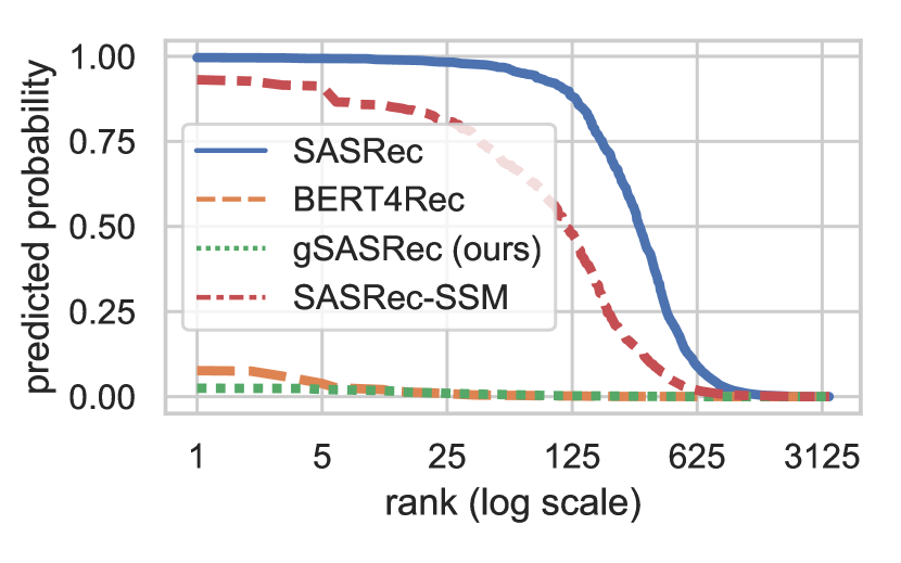
Figure 1. Predicted probability at different ranks for user 963 in MovieLens-1M. SASRec-SSM is a SASRec model trained with Sampled Softmax loss with 16 negatives.

We say that a model is overconfident in its predictions if its predicted probabilities $\hat{p}_{i}$ for highly-scored items are much larger compared to prior probabilities $P(i)$, i.e., $\hat{p}_{i}\gg P(i)$. In general, the magnitude of the relevance estimates are rank-invariant, i.e. do not affect the ordering of items, and hence they are rarely considered important when formulating a ranking model. In contrast, overconfidence is problematic only for the loss functions used to train the models, particularly when they directly model the interaction probability. Indeed, for some loss functions (such as pairwise BPR (Rendle et al., 2009) or listwise LambdaRank (Burges, 2010)), only the difference between the scores of paired items ($s_{i}-s_{j}$) is important, and therefore we cannot define overconfidence for these losses. However, these losses usually require algorithms that iteratively select “informative” negative samples, which are hard to apply with deep learning methods (see also Section 2.1). As discussed in Section 3.2, the prior probability distribution $P(i)$ cannot be directly observed, and therefore overconfidence may be hard to detect. However, in some cases, overconfidence may be obvious. For example, Figure 1 shows predicted probabilities by four different models for a sample user in the MovieLens-1M dataset. As can be seen from the figure, SASRec’s predicted probabilities for items at positions 1..25 are almost indistinguishable from 1. This is a clear sign of overconfidence: only one of these items can be the correct prediction, and therefore we expect the sum of probabilities to be approximately equal to 1, and not each individual probability. In fact, in this figure, the sum of all probabilities predicted by SASRec equals 338.03. In contrast, for BERT4Rec, the sum of probabilities equals exactly 1 (as the probabilities are computed using Softmax) and for our gSASRec (see Section 5.4) it is equal to 1.06. From the figure, we also see that a SASRec model trained with Sampled Softmax loss is also prone to overconfidence (sum of all probabilities equals 152.3).

Overconfidence for highly-ranked items is problematic: the model does not learn to distinguish these items from each other (all their predicted probabilities are approximately equal) and focuses on distinguishing top items from the bottom ones. The lack of focus on the top items contradicts our goal: we want the correct order of highly-ranked items and are not interested in score differences beyond a certain cutoff. Moreover, overconfidence is specifically problematic for BCE loss: if an item with high probability $\hat{p}_{i}\approx 1$ is selected as a negative (the chances of such an event are high when there are many high-scored items), $\log(1-{p}_{i})$ computed by the loss function tends to $-\infty$, causing numerical overflow problems and a training instability.

Next, we introduce gBCE loss, apply it for a theoretical analysis of BCE’s overconfidence, and show how gBCE mitigates the overconfidence problem.

5. Generalised Binary Cross Entropy and its properties

In this section we design gBCE and theoretically show that it can mitigate the overconfidence problem. In Section 5.1 we introduce gBCE and analyse its properties; in Section 5.2 we show that gBCE may be replaced with regular BCE loss with transformed positive scores, which may be more convenient in practice; in Section 5.3 we show how to reparametrise gBCE to make it independent from the chosen sampling rate; finally, in Section 5.4 we introduce gSASRec – an improved version of SASRec, which uses gBCE.

5.1. Generalised Binary Cross Entropy

We now introduce Generalised Binary Cross Entropy (gBCE) loss, which we use to analyse and mitigate overconfidence induced by negative sampling. We define gBCE, parameterised by $\beta$ as:

(8) $$\operatorname*{\mathcal{L}^{\beta}_{gBCE}}=-\frac{1}{|I_{k}^{-}|+1}\left(\log(\sigma^{\beta}(s_{i^{+}}))+\sum_{i\in I_{k}^{-}}\log(1-\sigma(s_{i}))\right).$$

gBCE differs from regular BCE loss in that it uses the generalised logistic sigmoid function (Richards, 1959; Pham et al., 2019) for the positive sample (sigmoid raised to the power of $\beta$). The power parameter $\beta\geq 0$ controls the shape of the generalised sigmoid. For example, when $\beta\approx 0$, the output of the generalised sigmoid becomes closer to 1 for all input scores. On the other hand, when $\beta=1$, BCE and gBCE are equal:

(9) $$\mathcal{L}^{1}_{gBCE}=\operatorname*{\mathcal{L}_{BCE}}$$

Similarly to BCE, gBCE is also a pointwise loss, and it considers the probability of interaction as a sigmoid transformation of the model score (Equation (1)). We now show the exact form of the relation between the prior probability $P(i)$ (which we desire to estimate, as we discuss in Section 3.2) and the modelled probabilities $\hat{p}_{i}=\sigma(s_{i})$, learned by a model trained with gBCE.

Theorem 5.1.

For every user in the dataset, let $P(i)$ be the prior probability distribution of the user interacting with item $i\in I$, $s=\{s_{1},...s_{|I|}\}$ are scores predicted by the model, $i^{+}$ is a positive sample selected by the user, $I_{k}^{-}=\{i^{-}_{1},i^{-}_{2},...,i^{-}_{k}\}$ - k randomly (uniformly, with replacement) sampled negatives, $\alpha=\frac{k}{|I^{-}|}$ - negative sampling rate. Then a recommender model, trained on a sufficiently large number of training samples using gradient descent and $\operatorname*{\mathcal{L}^{\beta}_{gBCE}}$ loss, will converge to predict score distribution $s$, so that

(10) $$\sigma(s_{i})=\frac{\beta P(i)}{\alpha-\alpha P(i)+\beta P(i)};\forall i\in I$$

Proof.

With a sufficiently large number of training samples, gradient descent converges to minimise the expectation of the loss function (Goodfellow et al., 2016, Ch. 4) (assuming the expectation has no local minima). Therefore, the predicted score distribution converges to the minimum of the expectation $\operatorname*{\mathbb{E}}\left[\operatorname*{\mathcal{L}^{\beta}_{gBCE}}\right]$:

(11) $$s=\operatorname*{arg\,min}_{s}\operatorname*{\mathbb{E}}\left[\operatorname*{\mathcal{L}^{\beta}_{gBCE}}\right]$$

Hence, our goal is to show that Theorem 5.1 is true if and only if the expectation $\operatorname*{\mathbb{E}}\left[\operatorname*{\mathcal{L}^{\beta}_{gBCE}}\right]$ is minimised.

To show that, we first rewrite the definition of $\operatorname*{\mathcal{L}^{\beta}_{gBCE}}$ (Equation (8)) as a sum of contributions for each individual item in $I$:

(12) $$\operatorname*{\mathcal{L}^{\beta}_{gBCE}}=\frac{1}{|I^{-}_{k}|+1}\sum_{i\in I}{\operatorname*{\mathcal{L}}}_{i}$$

where the contribution of each item, $\mathcal{L}_{i}$, is defined as follows:

(13) $${\operatorname*{\mathcal{L}}}_{i}=-(\operatorname*{\mathbb{I}}[i=i^{+}]\log(\sigma^{\beta}(s_{i}))+\sum_{j=1}^{k}\operatorname*{\mathbb{I}}[i=i^{-}_{j}]\log(1-\sigma{(s_{i})}))$$

The probability of an item being selected as a positive is defined by the prior distribution:

(14) $$P(\operatorname*{\mathbb{I}}[i=i^{+}])=P(i)$$

whereas the probability of an item being selected as $j^{th}$ negative is equal to the product of the probability of an item being negative and the negative sampling probability. If we apply a uniform sampling with a replacement for identifying negatives, then the sampling probability is always equal to $\frac{1}{|I^{-}|}$, so overall, the probability of selecting an item $i$ as the $j^{th}$ negative can be written as:

(15) $$P(\operatorname*{\mathbb{I}}[i=i^{-}_{j}])=\frac{1}{|I^{-}|}(1-P(i))$$

We can now calculate the expectations of each individual loss contribution $\operatorname*{\mathbb{E}}[{\operatorname*{\mathcal{L}}}_{i}]$:

$$\operatorname*{\mathbb{E}}[{\operatorname*{\mathcal{L}}}_{i}] =-(P(\operatorname*{\mathbb{I}}[i=i^{+}])\log(\sigma^{\beta}(s_{i}))+\sum_{j=1}^{k}P(\operatorname*{\mathbb{I}}[i=i^{-}_{j}])\log(1-\sigma{(s_{i})}))$$

         (By the definition of expectation)

$$=-(P(i)\log(\sigma^{\beta}(s_{i}))+\sum_{j=1}^{k}\frac{1}{|I^{-}|}(1-P(i))\log(1-\sigma{(s_{i})}))$$

         (Substituting Equations (14) and (15))

$$=-(P(i)\log(\sigma^{\beta}(s_{i}))+\frac{k}{|I^{-}|}(1-P(i))\log(1-\sigma{(s_{i})}))$$

         (The sum is just the same term repeated $$k$$ times)

$$=-(P(i)\log(\sigma^{\beta}(s_{i}))+\alpha(1-P(i))\log(1-\sigma{(s_{i})}))$$

(16)          (Substituting the sampling rate definition $$\alpha=\frac{k}{|I^{-}|}$$)

Differentiating Equation (16) on $\sigma(s_{i})$ we get:

(17) $$\frac{d\operatorname*{\mathbb{E}}[{\operatorname*{\mathcal{L}}}_{i}]}{d\sigma(s_{i})}=-\frac{\beta P(i)}{\sigma(s_{i})}+\frac{\alpha(1-P(i))}{1-\sigma(s_{i})}$$

Our goal is to minimise the expectation $\operatorname*{\mathbb{E}}[{\operatorname*{\mathcal{L}}}_{i}]$, so equating this derivative to zero and solving for $\sigma(s_{i})$ we obtain the value of $\sigma(s_{i})$, which minimises the expectation:

(18) $$\sigma(s_{i})=\frac{\beta P(i)}{\alpha-\alpha P(i)+\beta P(i)}$$

We now rewrite the expectation $\operatorname*{\mathbb{E}}\left[\operatorname*{\mathcal{L}^{\beta}_{gBCE}}\right]$ as the sum of its individual components:

(19) $$\operatorname*{\mathbb{E}}\left[\operatorname*{\mathcal{L}^{\beta}_{gBCE}}\right]=\operatorname*{\mathbb{E}}\left[\frac{1}{|I^{-}_{k}|+1}\sum_{i\in I}{\operatorname*{\mathcal{L}}}_{i}\right]=\frac{1}{|I^{-}_{k}|+1}\sum_{i\in I}\operatorname*{\mathbb{E}}\left[{\operatorname*{\mathcal{L}}}_{i}\right]$$

According to Equation (19), the expectation $\operatorname*{\mathbb{E}}\left[\operatorname*{\mathcal{L}^{\beta}_{gBCE}}\right]$ is minimised when, for each $i\in I$, the individual contributions $\operatorname*{\mathbb{E}}[{\operatorname*{\mathcal{L}}}_{i}]$ are minimised, i.e. when Equation (18) is true for each $i\in I$.  $\blacksquare$

We now use Theorem 5.1 to analyse properties of both regular and generalised Binary Cross-Entropy losses. First, we show that it is possible to train a model to estimate a prior distribution $P(i)$ exactly using gBCE loss.

Corollary 5.2.0.

If a model is trained using negative sampling with sampling rate $\alpha\leq 1$ and gBCE loss $\operatorname*{\mathcal{L}^{\beta}_{gBCE}}$ with $\beta=\alpha$, then the model converges to predict probabilities calibrated with the prior distribution:

(20) $$\sigma(s_{i})=P(i)$$

Proof.

We can obtain Equation (20) by substituting $\beta=\alpha$ in Equation (10).  $\blacksquare$

We now use Theorem 5.1 to analyse properties of regular Binary Cross-Entropy loss.

Corollary 5.3.0.

If a model is trained with BCE loss $\operatorname*{\mathcal{L}_{BCE}}$ and negative sampling, with sampling rate $\alpha$, then it converges to predict scores $s_{i}$ so that

(21) $$\sigma(s_{i})=\frac{P(i)}{\alpha-\alpha P(i)+P(i)}$$

Proof.

According to Equation (9), $\operatorname*{\mathcal{L}_{BCE}}$ is equal to $\operatorname*{\mathcal{L}^{\beta}_{gBCE}}$ with $\beta=1$. Substituting $\beta=1$ into Equation (10) we obtain Equation (21).  $\blacksquare$

We can now show that SASRec learns an overconfident score distribution:

Corollary 5.4.0.

The SASRec model with $\operatorname*{\mathcal{L}_{BCE}}$ and one negative per positive converges to yield scores $s_{i}$, such that:

(22) $$\sigma(s_{i})=\frac{P(i)|I|-P(i)}{P(i)|I|-2P(i)+1}$$

Proof.

SASRec uses one negative per positive, meaning that its sampling rate is equal to:

(23) $$\alpha=\frac{1}{|I|-1}$$

Substituting Equation (23) into Equation (21), we get Equation (22).  $\blacksquare$

Corollary 5.4 explains why SASRec tends to predict very high probabilities for top-ranked items: when an item has a higher-than-average probability of being selected ($P(i)\gg\frac{1}{|I|}$), the term $P(i)|I|$ dominates both the numerator and denominator of Equation (22), meaning that the predicted probability $\sigma(s_{i})$ will be very to close to 1.

5.2. Relation between BCE and gBCE

In Section 5.1 we showed that gBCE is equal to regular BCE loss when the power parameter $\beta$ is set to 1. We now show that these two loss functions have a deeper relation, which allows using well-optimised versions of BCE from deep learning frameworks instead of gBCE.

Theorem 5.5.

Let $s^{+}$ be the predicted score for a positive item and $s^{-}=\{s_{i^{-}_{1}},s_{i^{-}_{2}}..s_{i^{-}_{|I^{-}|}}\}$ be the predicted scores for the negative items. Then

(24) $$\operatorname*{\mathcal{L}^{\beta}_{gBCE}}(s^{+},s^{-})=\operatorname*{\mathcal{L}_{BCE}}(\gamma(s^{+}),s^{-})$$

where

(25) $$\gamma(s^{+})=\log\left(\frac{1}{\sigma^{-\beta}(s^{+})-1}\right)$$

Proof.

According to the definition of the logistic sigmoid function (Equation (1)),

$$\sigma(\gamma(s^{+})) =\frac{1}{e^{-\gamma(s^{+})}+1}$$

$$=\frac{1}{e^{-\log\left(\frac{1}{\sigma^{-\beta}(s^{+})-1}\right)}+1}$$

         (Substituting $$-\gamma(s^{+})$$ with its definition (Eq. (25)))

$$=\frac{1}{e^{\log\left(\sigma^{-\beta}(s^{+})-1\right)}+1}$$

         (Using properties of the $$\log(\cdot)$$ function)

$$=\frac{1}{\sigma^{-\beta}(s^{+})-1+1}$$

         (The exponent and the logarithm cancel each other out)

(26) $$=\frac{1}{\sigma^{-\beta}(s^{+})}=\sigma^{\beta}(s^{+})$$

Substituting $\sigma^{\beta}(s^{+})=\sigma(\gamma(s^{+}))$ into the definition of $\operatorname*{\mathcal{L}^{\beta}_{gBCE}}$ (Equation (8)) and taking into account the definition of $\operatorname*{\mathcal{L}_{BCE}}$ (Equation (7)) we get the desired equality:

$$\operatorname*{\mathcal{L}^{\beta}_{gBCE}}(s^{+},s^{-}) =-\frac{1}{|I^{-}_{k}|+1}\left(\log(\sigma^{\beta}(s_{i^{+}}))+\sum_{i\in I^{-}}\log(1-\sigma(s_{i}))\right)$$

$$=-\frac{1}{|I^{-}_{k}|+1}\left(\log(\sigma(\gamma(s^{+})))+\sum_{i\in I^{-}}\log(1-\sigma(s_{i}))\right)$$

$$=\operatorname*{\mathcal{L}_{BCE}}(\gamma(s^{+}),s^{-})$$

 $\blacksquare$

In practice, Theorem 5.2 allows us to transform the predicted positive scores by using Equation (25) and then train the model using the regular BCE loss, instead of using gBCE directly. This is actually preferable because many machine learning frameworks have efficient and numerically stable implementations for standard loss functions such as BCE loss. Indeed, in our implementation, we also rely on Equation (25) score transformation and regular BCE loss instead of using gBCE directly.

5.3. Calibration Parameter $t$

As shown in Section 5.1, setting the power parameter $\beta=1$ in gBCE resembles the regular BCE loss, whereas setting $\beta$ equal to the sampling rate $\alpha$ results in learning a fully calibrated distribution. This means that reasonable values of the $\beta$ parameter lie in the interval $[\alpha..1]$. In practice, we found working with this interval inconvenient: we usually do not control the $\alpha$ parameter directly and instead infer it from the number of negatives and size of the dataset. Similarly, the possible values of $\beta$ depend on these variables as well. To make the interval of possible values independent from $\alpha$, we control the power parameter $\beta$ indirectly with the help of a calibration parameter $t$, which adjusts $\beta$ as follows:

(27) $$\beta=\alpha\left(t\left(1-\frac{1}{\alpha}\right)+\frac{1}{\alpha}\right)$$

This substitution makes model configuration simpler: we select $t$ in the interval $[0..1]$, where $t=0$ ($\beta=1$) corresponds to regular BCE loss, and $t=1$ ($\beta=\alpha$) corresponds to the fully calibrated version of gBCE, which drives the model to estimate prior $P(i)$ exactly (according to Corollary 5.2).

5.4. gSASRec

gSASRec (generalised SASRec) is a version of the SASRec model with an increased number of negatives, trained with gBCE loss. Compared with SASRec, gSASRec has two extra hyperparameters: (i) number of negative samples per positive $k\in[1..|I^{-}|]$, and (ii) parameter $t\in[0..1]$, which indirectly controls the power parameter $\beta$ in gBCE using to Equation (27). In particular, when $k=1$ and $t=0$, gSASRec is the original SASRec model, as SASRec uses 1 negative per positive and gBCE becomes BCE when $t=0$. While our primary focus is on the SASRec model, it is possible to apply gBCE with other models; as an example, we use it also with BERT4Rec (see Section 6.2.4).

In the next section we empirically evaluate gSASRec and show that its generalisations over SASRec are indeed beneficial and allow it to match BERT4Rec’s performance, while retaining negative sampling.

6. Experiments

We design our experiments to answer the following research questions:

1. How does negative sampling affect BERT4Rec’s performance gains over SASRec?

2. What is the effect of gBCE on predicted item probabilities?

3. What is the effect of negative sampling rate and parameter $t$ on the performance of gSASRec?

4. How does gBCE loss affect the performance of SASRec and BERT4Rec models trained with negative sampling?

5. How does gSASRec perform in comparison to state-of-the-art sequential recommendation models?

6.1. Experimental Setup

6.1.1. Datasets

We experiment with three datasets: MovieLens-1M (Harper and Konstan, 2015), Steam (Pathak et al., 2017) and Gowalla (Cho et al., 2011). There are known limitations with MovieLens-1M (Petrov and Macdonald, 2022a, 2023a): it is a movies ratings dataset, and users may not rate items in the same order as they watch them, so the task, in this case, may be described as recommending movies to rate (and not to watch) next. However, it remains one of the most popular benchmarks for evaluating sequential recommender systems (Kang and McAuley, 2018; Sun et al., 2019; Petrov and Macdonald, 2022b; Qiu et al., 2022; Du et al., 2022), and more importantly, researchers use it consistently without additional preprocessing (the dataset is already preprocessed by its authors). This consistency allows us to compare results reported between different papers, and therefore we find experimenting with this dataset important. To stay consistent with previous research (Sun et al., 2019; Petrov and Macdonald, 2022b), we use preprocessed versions of the MovieLens-1M and Steam datasets provided in the BERT4Rec repository and do not apply any additional preprocessing. These datasets have relatively small numbers of items and therefore are suitable for training unsampled models such as BERT4Rec.

As a demonstration that gSASRec is suitable for larger datasets, we also use the Gowalla dataset, which is known to be problematic for BERT4Rec (Petrov and Macdonald, 2022a, 2023a). For this dataset, and following common practice (Kang and McAuley, 2018; Tang and Wang, 2018; Rendle et al., 2010; Sun et al., 2019; Petrov and Macdonald, 2022a, 2023a), we remove users with less than 5 interactions. Table 1 lists salient the characteristics of all three datasets. We split data using the standard leave-one-out approach, where we leave the last interaction for each user in the test dataset. Additionally, for each dataset, we randomly selected 512 users - for these users, we select their second last interaction and include them into a validation dataset, which we use for hyperparameter tuning as well as to control model early stopping.

Table 1. Experimental Datasets.

Dataset	Users	Items	Interactions
MovieLens-1M	6,040	3,416	999,611
Steam	281,428	13,044	3,488,885
Gowalla	86,168	1,271,638	6,397,903

6.1.2. Metrics

Until recently, a somewhat common approach in evaluating recommender systems on sampled metrics using only small number of items, but it has been shown that this leads to incorrect evaluation results in general (Krichene and Rendle, 2022; Cañamares and Castells, 2020), and specifically for sequential recommender systems (Dallmann et al., 2021; Petrov and Macdonald, 2022b). Hence, we always evaluate all item scores at the inference stage. Following (Petrov and Macdonald, 2022b), we evaluate our models using the popular Recall and NDCG metrics measured at cutoff 10. We also calculate Recall at cutoff 1, because according to Equation (22), we expect SASRec to be more overconfident on the highest-ranked metrics, and mitigating overconfidence should have a bigger effect on metrics measured at the highest cutoff.

6.1.3. Models

In our experiments, we compare gSASRec with the regular SASRec model, which serves as the backbone of our work. We also use BERT4Rec as a state-of-the-art baseline. For all models we set the sequence length to 200.

Additionally, we use two simple baselines: a non-personalised popularity model, which always recommends the most popular items; and the classic Matrix Factorisation model with BPR (Rendle et al., 2009) loss. Our implementation of SASRec (and gSASRec) are based on the original code, whereas our implementation of BERT4Rec is based on the more efficient implementation from our recent reproducibility paper (Petrov and Macdonald, 2022b). To ensure that the models are fully trained, we use an early stopping mechanism to stop training if NDCG@10 measured on the validation dataset has not improved for 200 epochs.

6.2. Results

6.2.1. RQ1. How does negative sampling affect BERT4Rec’s performance gains over SASRec

To answer our first research question, we train both BERT4Rec and SASRec on the Steam and MovieLens-1M datasets using the sampling strategies, which were originally used in these models: (i) one negative per positive and BCE loss (as in SASRec) and (ii) all negatives per positive and Softmax loss (as in BERT4Rec). We use the original training objectives for both architectures: item masking in BERT4Rec and sequence shifting in SASRec; we also retain the architecture differences in the models (i.e. we keep uni-directional attention in SASRec and bi-directional attention from BERT4rec). The results of our comparison are summarised in Table 2. The magnitude of SASRec and BERT4Rec results are aligned with those reported in (Petrov and Macdonald, 2022b). As can be seen from the table, in all four cases, changing of the sampling strategy from the one used by SASRec to the one used in BERT4Rec significantly improves effectiveness. For example, SASRec’s NDCG@10 on MovieLens-1M is improved from 0.131 to 0.169 (+29.0%) by removing negative sampling and applying Softmax loss. BERT4Rec achieves a larger improvement of NDCG@10 on Steam (0.0513 $\rightarrow$ 0.0746: +45.4%) when changing the sampling strategy from 1 negative to all negatives. In contrast, the effect of changing the architecture is moderate (e.g. statistically indistinguishable in 2 out of 4 cases), and frequently negative (3 cases out of four, 1 significant).

Table 2. Effects of model architecture and negative sampling on NDCG@10, for the MovieLens-1M (ML-1M) and Steam datasets. * denotes a significant change ($pvalue<0.05$) in NDCG@10 caused by negative sampling (comparing horizontally) or model architecture (comparing vertically).

Dataset	Negative sampling and loss function$\rightarrow$ Architecture$\downarrow$	1 negative per positive; BCE Loss (as SASRec)	No negative sampling; Softmax Loss (as BERT4Rec)	Negative sampling and loss effect
	SASRec	0.131	0.169	+29.0%*
	BERT4Rec	0.123	0.161	+30.8%*
ML-1M	Architecture effect	-6.1%	-4.7%
	SASRec	0.0581	0.0721	+24.1%*
	BERT4Rec	0.0513	0.0746	+45.4%*
Steam	Architecture effect	-11.7%*	+3.4%*

In the answer to RQ1, we conclude that the absence of negative sampling plays the key role in BERT4Rec’s success over SASRec, whereas any gain by applying BERT4Rec’s bi-directional attention architecture is only moderate and frequently negative. Therefore, the performance gains of BERT4Rec over SASRec can be attributed to the absence of negative sampling and Softmax loss and not to its architecture and training objective. This is contrary to the explanations of the original BERT4Rec authors in (Sun et al., 2019), who attributed its superiority to its bi-directional attention mechanism (on the same datasets). We now analyse how gBCE changes the distribution of predicted probabilities.

6.2.2. RQ2. Effect of gBCE on predicted interaction probabilities.

To analyse the effects of gBCE on predicted probabilities, we train three models: a regular SASRec model and two configurations of  gSASRec: a first with 64 negatives and $t=0.5$ and a second with 256 negatives and $t=1.0$. Our goal is to compare prior probabilities $P(i)$ with probabilities predicted by the model $\hat{p}_{i}$. As we discuss in Section 3.2, $P(i)$ is unknown, so direct measurement of such relation is hard. Hence, as a substitute for $P(i)$, we use the popular mean Precision@K metric, which according to Cormack et al. (Cormack et al., 1999) can be seen as a measurement of the conditional probability of an item being relevant, given its rank is less than K. We compare this metric with the average predicted probability of items retrieved at rank less than K. We perform this comparison for cutoffs K in the range [1..100]. Figure 2 displays the comparison results for MovieLens-1M and Steam datasets, illustrating the expected theoretical relationship between Precision@K and Predicted Probability@K based on Theorem 5.1.

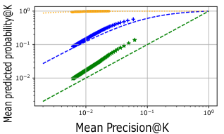
(a) MovieLens-1M

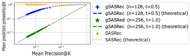
(b) Steam

Figure 2. Relation between Mean Precision@K metric and Mean predicted probability@K for cutoffs K in $[1..100]$ range. The figure also includes theoretical prediction for the relation according to Theorem 5.1.

Figure 2b shows that the theoretical prediction from Theorem 5.1 closely matches the observed relationship between Precision@K and Predicted Probability@K in the Steam dataset. In the MovieLens-1M dataset (Figure 2a), a slight discrepancy appears between the theoretical prediction and observed relationship, likely because the smaller number of users in the dataset doesn’t meet the requirement of Theorem 5.1 for an adequate amount of training samples.

Despite these small discrepancies, the relation follows the trends expected from our theoretical analysis. In particular, Figure 2 shows that as expected from Corollary 5.4, SASRec is indeed prone to overconfidence and on average predicts probabilities very close to 1 for all ranks less than 100. In contrast, the probabilities predicted by gSASRec are considerably less than 1. For example, for MovieLens-1M, gSASRec trained with 128 negatives and $t=0.5$, on average predicts probability 0.57 at K=1, while the version with 256 negatives and $t=1.0$ predicts probability 0.13 at the same cutoff. Together, this analysis shows that gSASRec trained with gBCE successfully mitigates the overconfidence problem of SASRec. Furthermore, from the figure we also see that when parameter $t$ is set to 1, the mean predicted probability is well-calibrated with mean precision at all rank cutoffs (particularly on the Steam dataset). This is well-aligned with Corollary 5.2, which states that when parameter $\beta$ in gBCE is set equal to the sampling rate (i.e. setting parameter $t=1$) results in learning in fully calibrated probabilities. Overall in answer to RQ2, we conclude that gBCE successfully mitigates the overconfidence problem, and in a manner that is well-aligned with our theoretical analysis. We next turn to the impact of gBCE on effectiveness.

6.2.3. RQ3. Effect of negative sampling rate and parameter $t$ on the performance of gSASRec

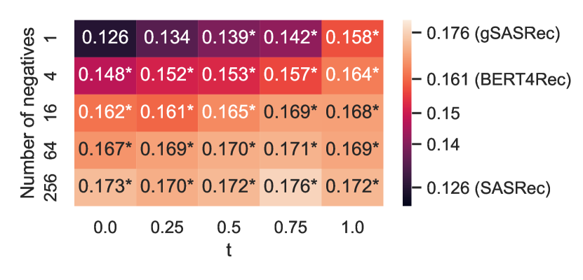
Figure 3. gSASRec: Effect of varying number of negatives and calibration parameter $t$ on NDCG@10, MovieLens-1M. * denotes a significant improvement over SASRec ($pvalue<0.05$, Bonferroni multiple test correction).

In comparison to SASRec, gSASRec has two additional hyperparameters: the number of negative samples and the parameter $t$, which adjusts probability calibration. To explore the impact of these parameters on performance, we conduct a grid search: selecting the negative sample count from [1, 4, 16, 64, 256] and the calibration parameter $t$ from [0, 0.25, 0.5, 0.75, 1.0].

Figure 3 portrays our grid search on MovieLens-1M (on others datasets we observed a similar pattern and omit their figures for brevity). From the figure, we observe that, as expected from the theoretical analysis, both $t$ and the number of negatives have a positive effect on model effectiveness. For example, when the number of negatives is set to 1, varying $t$ from 0 to 1 allows increasing NDCG@10 from 0.126 to 0.158 (+25%, significant, compared to SASRec, which is also gSASRec with 1 negative and calibration $t=0$). Interestingly, the result of gSASRec with 1 negative and $t=1$ is similar to what BERT4Rec achieves with all negatives (0.158 vs. 0.161: -1.86%, not significant). We also observe that when the number of negatives is higher, setting a high value of $t$ is less important. For example, when the model is trained with 256 negatives (7.49% sampling rate), the model achieves high effectiveness with all values of $t$. This is also not surprising – by design, more negative samples and higher values of $t$ should have a similar effect in gBCE. During our experiments, we also observed that setting parameter $t$ very close to 1 also increased the training time of the model. Keeping this in mind, in practical applications we recommend setting $t$ between 0.75 and 0.9, and the number of negatives between 128 and 256 – this combination works well on all datasets, converging to results that are close to the best observed without increasing training time. This answers RQ3.

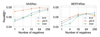
(a) Recall@1

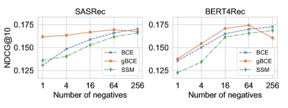
(b) NDCG@10

Figure 4. Performance of SASRec and BERT4Rec architectures, trained on the MovieLens-1M dataset with a variable number of negatives and various loss functions. BCE is a classic Binary Cross Entropy Loss, gBCE - Generalised Binary Cross-entropy (t=1.0), SSM - Sampled Softmax Loss with uniform sampling.

6.2.4. RQ4. Effect of gBCE loss on negatively sampled SASRec and BERT4Rec

To investigate the effect of gBCE on SASRec and BERT4Rec models with negative sampling , we train the models with the number of negative samples selected from [1, 4, 16, 64, 256] and the loss function selected from [BCE, gBCE, Sampled Softmax Loss (SSM)] on the MovieLens-1M dataset. In this experiment, we use a fully-calibrated version of gBCE ($t=1.0$). Figure 4 summarises the results of the experiment. As we can see from the figure, gBCE performs better than both BCE and Sampled Softmax loss when the number of negatives is small. For example, for BERT4Rec trained with 4 negatives, gBCE has a higher Recall@1 (0.059) than both BCE (0.055; -5.8% compared with gBCE) and Sampled Softmax (0.046, -20%) and has the highest NDCG@10 of 0.154, while BCE has NDCG@10 of 0.150 (-2.6% compared with gBCE) and Sampled Softmax has NDCG@10 of 0.134 (-12.9%). In the case of SASRec, the difference is even larger when the number of negatives is small (recall that SASRec trained with gBCE is also gSASRec). For example, with 16 negatives, gBCE achieves Recall@1 0.0769, BCE achieves 0.0673 (-12.5%), and Sampled Softmax achieves 0.0635 (-17.5%). We hypothesise that gBCE affects SASRec more than BERT4Rec due to their training objectives. SASRec predicts the next item in a sequence, while BERT4Rec predicts randomly masked items. Consequently, altering SASRec’s loss function directly impacts its performance in next-item prediction. In contrast, changing BERT4Rec’s loss function only affect the masking task which is less directly related to the next item prediction task (Petrov and Macdonald, 2022a, 2023a). On the other hand, when more negatives are sampled, gBCE becomes less beneficial. For example, with 256 negatives, all three loss functions achieve similar NDCG@10 (0.1674 gBCE; 0.1703 (+1.7%) BCE and 0.1660 (-0.08%) Sampled Softmax). This is an expected result because 256 negatives represent a significant proportion of all negatives (7.5%), and overconfidence becomes less of an issue for BCE and Sampled Softmax.

In conclusion, for RQ4, gBCE outperforms BCE and Sampled Softmax in SASRec and BERT4Rec with few negatives; improvement is larger in SASRec. However, with many negatives, traditional loss functions like BCE and Sampled Softmax work well unaltered, but high sampling rates are impractical due to memory and computational constraints.

6.2.5. RQ5. gSASRec performance in comparison to state-of the-art sequential recommendation models.

To answer our last research question, we compare gSASRec with the baseline models. We also add to comparison a version of SASRec trained with full Softmax (without sampling) because, as we discuss in RQ1, it exhibits SOTA performance; however, we omit non-standard versions of BERT4Rec and SASRec trained with BCE or Sampled Softmax, because as we report in RQ4 they are not beneficial compared to gBCE. We also exclude BERT4Rec with gBCE from our analysis because, as per RQ4, gSASRec achieves superior results when measured by Recall@1 and similar results when evaluated by NDCG@10. After tuning hyperparameters on the validation set, we report the results of gSASRec with 128 negatives and $t=0.9$ for Steam and Gowalla, and with 256 negatives and $t=0.75$ for MovieLens-1M. Table 3 summarises the results of our evaluation. The table shows that gSASRec achieved the best or the second best result on all datasets according to all metrics. Indeed, on the smaller datasets (MovieLens and Steam), where we were able to train BERT4Rec and SASRec without sampling, gSASRec performs similarly to the best unsampled model (e.g.  +4.1% NDCG@10 on MovieLens-1M compared to SASRec-Softmax (not significant) or -1.74% compared to BERT4Rec on Steam, significant). Interestingly, on MovieLens-1M, both SASRec-Softmax (our version of SASRec trained without negative sampling) and gSASRec significantly improve Recall@1, suggesting that at least in some cases SASRec’s unidirectional architecture may be beneficial. This also echoes our observations while analysing RQ1.

Table 3. Evaluation results. Bold denotes the best model on the dataset for that metric and underlined is the second-best model. * denotes a significant difference with the best-performing model ($pvalue<0.05$). SASRec-Softmax is a SASRec-based model trained without negative sampling and Softmax loss (as BERT4Rec).

Model

Datasets

MovieLens-1M

Steam

Gowalla

Category

Model

Negative Sampling

Loss

Recall @1

Recall @10

NDCG @10

Time (min)

Recall @1

Recall @10

NDCG @10

Time (min)

Recall @1

Recall @10

NDCG @10

Time (min)

Baselines

Popularity

N/A

N/A

0.005*

0.036*

0.017*

0.0

0.0077*

0.0529*

0.0268*

0.0

0.0011*

0.0081*

0.0041*

0.1

MF-BPR

Yes

BPR

0.010*

0.075*

0.037*

0.1

0.0071*

0.0393*

0.0206*

0.4

0.0083*

0.0282*

0.0170*

2.1

Unsampled

BERT4Rec

No

Softmax

0.058*

0.294

0.161*

86

0.0281

0.1379

0.0746

642

Infeasible (requires $>$100GB of GPU memory, see Section 1)

SASRec-Softmax

No

Softmax

0.073

0.293

0.169

9

0.0280

0.1323*

0.0721*

80

Sampled

SASRec

Yes

BCE

0.046*

0.247*

0.131*

13

0.0193*

0.1121*

0.0581*

32

0.0505*

0.1831*

0.1097*

145

gSASRec

Yes

gBCE

0.082

0.300

0.176

23

0.0283

0.1355

0.0735

58

0.0782

0.2590

0.1616

191

Crucially, gSASRec always significantly outperforms the regular SASRec model (+34% NDCG@10 on MovieLens-1M, +26% on Steam, +47% on Gowalla). The result on Gowalla is particularly important, as it demonstrates that gSASRec is suitable for datasets with more than 1 million items, and it improves SASRec’s results by a large margin on this large dataset. From Table 3 we also see that all versions of SASRec (including gSASRec) require less training time than BERT4Rec. For example, on MovieLens, gSASRec is 73.2% faster to train compared to BERT4Rec (23 minutes vs. 85 minutes) and, on Steam, gSASRec is 90.9% faster (58 minutes vs.  642 minutes). However, we also see that gSASRec requires more training time than SASRec (e.g. 58 vs. 32 minutes on Steam); we explain that by the fact that more accurate probabilities estimation with gBCE requires more training epochs to converge (238 epochs vs. 170 epochs in our experiment).

Finally, for MovieLens-1M, we compare the results achieved by gSASRec with those of the most recently proposed models in the literature, which report the best results, namely ALBERT4Rec (Petrov and Macdonald, 2022b) (an effective model similar to BERT4Rec, but based on ALBERT (Lan et al., 2020)), and two contrastive models: DuoRec (Qiu et al., 2022), and CBiT (Du et al., 2022). All papers from our selection the use the same data-splitting strategy and unsampled metrics, so the results are comparable. Table 4 summarises this comparison. As we can see from the table, all these publications report Recall@10 close to 0.3, which is similar to what we obtain with gSASRec. However, only gSASRec achieves an NDCG@10 above 0.17. Furthermore, as observed from Figure 3, this result is not a one-off occurrence but a consistent outcome when the model is trained with 256 negatives, making it unlikely to be a statistical fluctuation. This is likely due to its better focus on highly-ranked items, as gBCE is specifically designed for improving overconfidence in highly-scored items.

Overall, our experiments show that gSASRec performs on par with SOTA models, retaining the negative sampling required for use on big catalogues and converging faster than BERT4Rec.

7. Conclusions

Table 4. Comparison of gSASRec with recent reported results on MovieLens-1M. Bold indicates the best value.

	Recall@10	NDCG@10
DuoRec (Qiu et al., 2022)	0.294	0.168
ALBERT4Rec (Petrov and Macdonald, 2022b)	0.300	0.165
CBiT (Du et al., 2022)	0.301	0.169
gSASRec	0.300	0.176

In this paper, we studied the impact of negative sampling on sequential recommender systems. We showed (theoretically and empirically) that negative sampling coupled with Binary Cross-Entropy loss (a popular combination used by many sequential models) leads to a shifted score distribution, called overconfidence. We showed that overconfidence is the only reason why SASRec underperforms compared to the state-of-the-art BERT4Rec. Indeed, when we control for negative sampling, the two models perform similarly. We proposed a solution to the overconfidence problem in the form of gBCE and theoretically proved that it can mitigate overconfidence. We further proposed gSASRec, which uses gBCE, and experimentally showed that it can significantly outperform the best unsampled models (e.g. +9.47% NDCG@10 on the MovieLens-1M dataset compared to BERT4Rec) requiring less training time (e.g. -90.9% on the Steam dataset compared to BERT4Rec), while also being suitable for large-scale datasets. We also showed that gBCE may be beneficial for BERT4Rec if it is trained with negative sampling (e.g. +7.2% compared to BCE when trained with 4 negatives). The theory and methods presented in this paper could also be applied to not just sequential recommendation models but also to other types of recommendation as well as to NLP or search tasks – we leave these directions to future work.

References

- (1)
- Acquavia et al. (2023) Antonio Acquavia, Nicola Tonellotto, and Craig Macdonald. 2023. Static Pruning for Multi-Representation Dense Retrieval. In Proc. DocEng.
- Burges (2010) Christopher Burges. 2010. From RankNet to LambdaRank to LambdaMART: An Overview. Learning 11 (Jan. 2010).
- Cañamares and Castells (2020) Rocío Cañamares and Pablo Castells. 2020. On Target Item Sampling in Offline Recommender System Evaluation. In Proc. RecSys. 259–268.
- Chen et al. ([n. d.]) Yongjun Chen, Jia Li, Zhiwei Liu, Nitish Shirish Keskar, Huan Wang, Julian McAuley, and Caiming Xiong. [n. d.]. Generating Negative Samples for Sequential Recommendation. arXiv:2208.03645 [cs]
- Cho et al. (2011) Eunjoon Cho, Seth A. Myers, and Jure Leskovec. 2011. Friendship and Mobility: User Movement in Location-Based Social Networks. In Proc. KDD. 1082.
- Cormack et al. (1999) Gordon V. Cormack, Ondrej Lhotak, and Christopher R. Palmer. 1999. Estimating Precision by Random Sampling. In Proc. SIGIR. 273–274.
- Dallmann et al. (2021) Alexander Dallmann, Daniel Zoller, and Andreas Hotho. 2021. A Case Study on Sampling Strategies for Evaluating Neural Sequential Item Recommendation Models. In Proc. RecSys. 505–514.
- Devlin et al. (2019) Jacob Devlin, Ming-Wei Chang, Kenton Lee, and Kristina Toutanova. 2019. BERT: Pre-training of Deep Bidirectional Transformers for Language Understanding. In Proc. of NAACL-HLT. 4171–4186.
- Dodge et al. (2021) Jesse Dodge, Maarten Sap, Ana Marasović, William Agnew, Gabriel Ilharco, Dirk Groeneveld, Margaret Mitchell, and Matt Gardner. 2021. Documenting Large Webtext Corpora: A Case Study on the Colossal Clean Crawled Corpus. In Proc. EMNLP. 1286–1305.
- Du et al. (2022) Hanwen Du, Hui Shi, Pengpeng Zhao, Deqing Wang, Victor S. Sheng, Yanchi Liu, Guanfeng Liu, and Lei Zhao. 2022. Contrastive Learning with Bidirectional Transformers for Sequential Recommendation. In Proc. CIKM. 396–405.
- Goodfellow et al. (2016) Ian Goodfellow, Yoshua Bengio, and Aaron Courville. 2016. Deep Learning. MIT Press.
- Harper and Konstan (2015) F. Maxwell Harper and Joseph A. Konstan. 2015. The MovieLens Datasets: History and Context. ACM Transactions on Interactive Intelligent Systems (TiiS) 5, 4 (Dec. 2015), 19:1–19:19.
- Heaps (1978) H. S. Heaps. 1978. Information Retrieval: Computational and Theoretical Aspects. Academic Press, Inc., USA.
- Hidasi et al. (2016) Balázs Hidasi, Alexandros Karatzoglou, Linas Baltrunas, and Domonkos Tikk. 2016. Session-Based Recommendations with Recurrent Neural Networks. In Proc. ICLR.
- Jean et al. (2015) Sébastien Jean, Kyunghyun Cho, Roland Memisevic, and Yoshua Bengio. 2015. On Using Very Large Target Vocabulary for Neural Machine Translation. In Proc. ACL-IJCNLP. 1–10.
- Ji et al. (2020) Yitong Ji, Aixin Sun, Jie Zhang, and Chenliang Li. 2020. A Re-visit of the Popularity Baseline in Recommender Systems. In Proc. SIGIR. 1749–1752.
- Kang and McAuley (2018) Wang-Cheng Kang and Julian McAuley. 2018. Self-Attentive Sequential Recommendation. In Proc. ICDM. 197–206.
- Krichene and Rendle (2022) Walid Krichene and Steffen Rendle. 2022. On Sampled Metrics for Item Recommendation. Commun. ACM 65, 7 (June 2022), 75–83.
- Lan et al. (2020) Zhenzhong Lan, Mingda Chen, Sebastian Goodman, Kevin Gimpel, Piyush Sharma, and Radu Soricut. 2020. ALBERT: A Lite BERT for Self-supervised Learning of Language Representations. In Proc. ICLR.
- Lin et al. (2022) Jimmy Lin, Rodrigo Nogueira, and Andrew Yates. 2022. Pretrained Transformers for Text Ranking: BERT and Beyond. Springer International Publishing.
- Murphy (2022) Kevin P. Murphy. 2022. Probabilistic Machine Learning: An Introduction. The MIT Press, Cambridge, Massachusetts.
- Pathak et al. (2017) Apurva Pathak, Kshitiz Gupta, and Julian McAuley. 2017. Generating and Personalizing Bundle Recommendations on Steam. In Proc. SIGIR. 1073–1076.
- Pellegrini et al. (2022) Roberto Pellegrini, Wenjie Zhao, and Iain Murray. 2022. Don’t Recommend the Obvious: Estimate Probability Ratios. In Proc. RecSys. 188–197.
- Petrov and Macdonald (2022a) Aleksandr Petrov and Craig Macdonald. 2022a. Effective and Efficient Training for Sequential Recommendation Using Recency Sampling. In Proc. RecSys. 81–91.
- Petrov and Macdonald (2022b) Aleksandr Petrov and Craig Macdonald. 2022b. A Systematic Review and Replicability Study of BERT4Rec for Sequential Recommendation. In Proc. RecSys. 436–447.
- Petrov and Macdonald (2023a) Aleksandr Petrov and Craig Macdonald. 2023a. RSS: Effective and Efficient Training for Sequential Recommendation Using Recency Sampling. ACM Transactions on Recommender Systems (TORS) (2023).
- Petrov and Macdonald (2023b) Aleksandr V Petrov and Craig Macdonald. 2023b. Generative Sequential Recommendation with GPTRec. In Proc. GenIR@SIGIR.
- Pham et al. (2019) Luan Thanh Pham, Erdinc Oksum, Thanh Duc Do, Minh Le-Huy, Minh Duc Vu, and Vinh Duc Nguyen. 2019. LAS: A Combination of the Analytic Signal Amplitude and the Generalised Logistic Function as a Novel Edge Enhancement of Magnetic Data. Contributions to Geophysics & Geodesy 49, 4 (2019), 425–440.
- Qiu et al. (2022) Ruihong Qiu, Zi Huang, Hongzhi Yin, and Zijian Wang. 2022. Contrastive Learning for Representation Degeneration Problem in Sequential Recommendation. In Proc. WSDM. 813–823.
- Rendle (2022) Steffen Rendle. 2022. Item Recommendation from Implicit Feedback. In Recommender Systems Handbook. 143–171.
- Rendle and Freudenthaler (2014) Steffen Rendle and Christoph Freudenthaler. 2014. Improving Pairwise Learning for Item Recommendation from Implicit Feedback. In Proc. WSDM.
- Rendle et al. (2009) Steffen Rendle, Christoph Freudenthaler, Zeno Gantner, and Lars Schmidt-Thieme. 2009. BPR: Bayesian Personalized Ranking from Implicit Feedback. In Proc. UAI.
- Rendle et al. (2010) Steffen Rendle, Christoph Freudenthaler, and Lars Schmidt-Thieme. 2010. Factorizing Personalized Markov Chains for Next-Basket Recommendation. In Proc. WWW. 811.
- Richards (1959) F. J. Richards. 1959. A Flexible Growth Function for Empirical Use. Journal of Experimental Botany 10, 2 (1959), 290–301.
- Stolcke (1998) A. Stolcke. 1998. Entropy-Based Pruning of Backoff Language Models. In Proc. Broadcast News Tanscription and Understanding Workshop. 270–274.
- Sun et al. (2019) Fei Sun, Jun Liu, Jian Wu, Changhua Pei, Xiao Lin, Wenwu Ou, and Peng Jiang. 2019. BERT4Rec: Sequential Recommendation with Bidirectional Encoder Representations from Transformer. In Proc. CIKM. 1441–1450.
- Tang and Wang (2018) Jiaxi Tang and Ke Wang. 2018. Personalized Top-N Sequential Recommendation via Convolutional Sequence Embedding. In Proc. WSDM. 565–573.
- Vaswani et al. (2017) Ashish Vaswani, Noam Shazeer, Niki Parmar, Jakob Uszkoreit, Llion Jones, Aidan N Gomez, Łukasz Kaiser, and Illia Polosukhin. 2017. Attention Is All You Need. In Proc. NeurIPS.
- Wei et al. (2022) Hongxin Wei, Renchunzi Xie, Hao Cheng, Lei Feng, Bo An, and Yixuan Li. 2022. Mitigating Neural Network Overconfidence with Logit Normalization. In Proc. ICML.
- Weston et al. (2011) Jason Weston, Samy Bengio, and Nicolas Usunier. 2011. Wsabie: Scaling Up To Large Vocabulary Image Annotation. In Proc. IJCAI.
- Wu et al. (2022) Jiancan Wu, Xiang Wang, Xingyu Gao, Jiawei Chen, Hongcheng Fu, Tianyu Qiu, and Xiangnan He. 2022. On the Effectiveness of Sampled Softmax Loss for Item Recommendation. arXiv:2201.02327 [cs]
- Wu et al. (2016) Yonghui Wu, Mike Schuster, Zhifeng Chen, Quoc V. Le, Mohammad Norouzi, Wolfgang Macherey, Maxim Krikun, Yuan Cao, Qin Gao, Klaus Macherey, Jeff Klingner, Apurva Shah, Melvin Johnson, Xiaobing Liu, Łukasz Kaiser, Stephan Gouws, Yoshikiyo Kato, Taku Kudo, Hideto Kazawa, Keith Stevens, George Kurian, Nishant Patil, Wei Wang, Cliff Young, Jason Smith, Jason Riesa, Alex Rudnick, Oriol Vinyals, Greg Corrado, Macduff Hughes, and Jeffrey Dean. 2016. Google’s Neural Machine Translation System: Bridging the Gap between Human and Machine Translation. arXiv:1609.08144 [cs]
- Xie et al. (2022) Xu Xie, Fei Sun, Zhaoyang Liu, Shiwen Wu, Jinyang Gao, Jiandong Zhang, Bolin Ding, and Bin Cui. 2022. Contrastive Learning for Sequential Recommendation. In Proc. ICDE. 1259–1273.
- Yuan et al. (2016) Fajie Yuan, Guibing Guo, Joemon M. Jose, Long Chen, Haitao Yu, and Weinan Zhang. 2016. LambdaFM: Learning Optimal Ranking with Factorization Machines Using Lambda Surrogates. In Proc. CIKM. 227–236.
- Yuan et al. (2019) Fajie Yuan, Alexandros Karatzoglou, Ioannis Arapakis, Joemon M. Jose, and Xiangnan He. 2019. A Simple Convolutional Generative Network for Next Item Recommendation. In Proc. WSDM. 582–590.
- Zhou et al. (2020) Kun Zhou, Hui Wang, Wayne Xin Zhao, Yutao Zhu, Sirui Wang, Fuzheng Zhang, Zhongyuan Wang, and Ji-Rong Wen. 2020. S3-Rec: Self-Supervised Learning for Sequential Recommendation with Mutual Information Maximization. In Proc. CIKM. 1893–1902.