Cosmological electromagnetic hopfions

Abstract

It is shown that any mathematical solution for null electromagnetic field knots in flat spacetime is also a null field knotted solution for cosmological electromagnetic fields that may be obtained by replacing the time $t\rightarrow\tau=\int dt/a$, where $a=a(t)$ is the scale factor of the Universe described by the Friedman-Lemaître-Robertson-Walker (FLRW) cosmology, and by adequately rewriting the (empty flat spacetimes) electromagnetic fields solutions in a medium defined by the FLRW metric. We found that the dispersion (evolutoion) of electromagnetic hopfions is faster on cosmological scenarios. We discuss the implications of these results for different cosmological models.

I Introduction

Hopfions are knotted topological solitons which are solutions to different kinds of field equations in physics, which are best described in terms of the Hopf map hopf . Although the main purpose of this work is to deal with electromagnetic Hopfions on both empty flat spacetime and on cosmological backgrounds, it is only fair to say that Hopf map can be found in physics in many different subjects ranging from fluid dynamics to superconductivity to quantum computing to electromagnetism to skyrmions. Some of these topics are discussed in the article “The Hopf fibration–seven times in physics” by Urbantke urbantke . Furthermore, several hopfions structures have been successfully produced in laboratory Jung-Shen ; particle ; Ackerman ; BGg ; Reynolds .

To the best of our knowledge, the first electromagnetic Hopfions in empty flat spacetime were found by Rañada in 1989 rañada1 ; rañada2 ; rañada3 ; rañada4 ; rañada5 . Rañada started with by defining the initial ($t=0$) values of the electromagnetic fields ${\bf E}(x,y,z,0)$ and ${\bf B}(x,y,z,0)$ (which satisfy the initial value constraints) as solutions to the Hopf map. To get the time dependent fields ${\bf E}(x,y,z,t)$ and ${\bf B}(x,y,z,t)$ is sufficient to propagate the initial value fields using the Fourier transform to satisfy the full set of Maxwell equations. It is worth noting that hopfions electromagnetic fields are null, i.e., ${\bf E}({\bf r},t)\cdot{\bf B}({\bf r},t)=0$, and ${\bf E}({\bf r},t)\cdot{\bf E}({\bf r},t)={\bf B}({\bf r},t)\cdot{\bf B}({\bf r},t)$.

It is the porpuse of this work to show that a slightly modified form of (empty flat spacetime) Rañada’s Hopfion produces an electromagnetic cosmological Hopfion on a FLRW (empty curved spacetime) background. This cosmological electromagnetic hopfions have a dynamical evolution that depends on the cosmological model in which develop. This work is in the same spirit of the results found for electromagnetic hopfions in de Sitter spacetime Grzelaa . However, in here, we present a study of a more general span of different cosmological models, described by the Friedman-Lemaître-Robertson-Walker (FLRW) metric. This works can be done straightforwardly by taking advantage of the conformal flat nature of Maxwell equation under the FLRW metric. Thus, any hopfion solution of flat spacetime Maxwell equation will be also a solution of Maxwell equations in cosmology, evolving on a cosmological time, and with similar properties to the ones discussed here.

Below, we study a hopfion in an expanding Universe filled by a perfect fluid with positive equation of state. Also, we explore the form how a hopfion disperse in a accelerated expanding Universe filled by a cosmological constant that plays the role of dark energy. In all these cases, we show that electromagnetic hopfions evolve (and disperse) faster than in flat spacetime, as the cosmological time that determines the structure of the hopfion runs faster than the coordinate time of flat spacetime.

In Sec. II, we present the general formulation of Maxwell equations in FLRW cosmology. In Sec. III we present a simple hopfion solution for general cosmology, and we analyze its behavior under different cosmological scenarios. Finally, in Sec. IV we discuss these findings.

II Maxwell equations in FRW cosmology

In curved spacetime, Maxwell equations are written as

$$\nabla_{\mu}F^{\mu\nu}=0\,,\quad\nabla_{\mu}F^{*\mu\nu}=0\,,$$ (1)

in terms of covariant derivative operators for a spacetime metric $g_{\mu\nu}$, for the electromagnetic tensor $F_{\mu\nu}$ (and its dual $F_{\mu\nu}^{*}$). We now define the vectorial electric fields as $E_{i}=F_{i0}$, and $D^{i}=\sqrt{-g}F^{0i}$. Similarly, we define and magnetic fields as $B^{i}=\varepsilon^{0ijk}F_{jk}$ and $\varepsilon^{0ijk}H_{k}=\sqrt{-g}F^{ij}$. They fulfill the relations $D^{i}=-\sqrt{-g}({g^{ij}}/{g^{00}})E_{j}+\varepsilon^{0ijk}({g_{0j}}/{g_{00}})H_{k}$, and $B^{i}=-\sqrt{-g}({g^{ij}}/{g^{00}})H_{j}-\varepsilon^{0ijk}({g_{0j}}/{g_{00}})E_{k}$ Plebanksi ; Felice ; mass1 ; mass2 ; asenjohojman .

In the following we consider a cosmological model described by the FLRW metric $g_{\mu\nu}={\mbox{diag}}(-1,a^{2},a^{2},a^{2})$ (in Cartesian coordinates), where $a=a(t)$ is the scale factor of the Universe, in terms of the proper time $t$. In this case, we have that ${\bf D}=a{\bf E}$, and ${\bf B}=a{\bf H}$. In this way, the Maxwell equations (1) become

$$i\frac{\partial\textbf{\emph{F}}}{\partial\tau} = \nabla\times\textbf{\emph{F}}$$ (2)

where $\textbf{\emph{F}}={\bf D}+i{\bf B}=a{\bf E}+ia{\bf H}$ is Riemann–Silberstein vector for the FLRW system, written in terms of the conformal time

$$\tau=\int\frac{dt}{a}.$$ (3)

The previous calculation shows that, as the FLRW cosmology is conformally flat, any solution of the source-free Maxwell equations in Minkowski spacetime will remain a solution in FLRW spacetime. In this case, the energy $\int d^{3}r\,\textbf{\emph{F}}^{*}\cdot\textbf{\emph{F}}$ of any solution is conserved in the cosmological time.

III Cosmological hopfions

All flat spacetime hopfions solutions of Maxwell equation will be solution of the cosmological FLRW Maxwell equations (2), now for the cosmological time $\tau$. Several null solutions of Maxwell equations are known for flat spacetimes (see, for example, Refs. rañada1 ; rañada2 ; rañada3 ; rañada4 ; rañada5 ; iwoff3 ; besieris ; irvine ; particle ; array ; TRAUTMAN ; amy ; irvine2 ; hoyos ). Due to the conformally flat nature of FLRW cosmology, all these solutions are also cosmological electromagnetic hopfions solutions, with the corresponding change in time. This is not a trivial change, as the cosmological time $\tau$ depends on the cosmological Universe where electromagnetic fields develop. Thereby, electromagnetic hopfions evolve different in diverse cosmological settings compared to flat spacetime.

In here, we display this behavior by studying a simplest hopfion solution besieris ; irvine . The cosmological electrogmagnetic hopfion solution of Eqs. (2) is

$${\bf D}=\frac{\nabla\zeta\times\nabla{\bar{\zeta}}}{4\pi i(1+{\bar{\zeta}}\,\zeta)^{2}}\,,\quad{\bf B}=\frac{\nabla\eta\times\nabla{\bar{\eta}}}{4\pi i(1+{\bar{\eta}}\,\eta)^{2}}\,,$$ (4)

where (in Cartesian coordinates, and conformal time $\tau$)

$$\zeta(\tau,x,y,z) = \frac{Ax+y\,\tau+i\left(Az+(A-1)\tau\right)}{x\,\tau-Ay+i\left(A(A-1)-z\,\tau\right)}\,,$$

$$\eta(\tau,x,y,z) = \frac{Az+(A-1)\tau+i\left(x\,\tau-Ay\right)}{Ax+y\,\tau+i\left(A(A-1)-z\,\tau\right)}\,,$$

$$A(\tau,x,y,z) = \left(x^{2}+y^{2}+z^{2}+1-\tau^{2}\right)/2\,,$$ (5)

and ${\bar{\eta}}$, ${\bar{\zeta}}$ are the complex conjugated of such functions. This hopfion solution fulfills ${\bf B}\cdot{\bf D}=0={\bf H}\cdot{\bf E}$, and $|{\bf B}|^{2}=|{\bf D}|^{2}=a^{2}|{\bf H}|^{2}=a^{2}|{\bf E}|^{2}$.

The nonlinearity of the $t\rightarrow\ \tau$ transformation produces significant changes in the evolution of hopfions. A Universe filled with perfect fluid, with a proper energy to pressure ratio given by $w$, has a scale factor given by $a(t)=(t/t_{0})^{2/(3+3w)}$ ryden , with $0<t<t_{0}$, where $t_{0}$ is the current age of the Universe. Thus, for this case, the conformal time becomes

$$\tau=\frac{3(1+w)\,t}{1+3w}\left(\frac{t_{0}}{t}\right)^{\frac{2}{3+3w}}\,.$$ (6)

In here, we consider only normal fluids with $0<w<1$. Due to this, then $\tau>t$ always. Therefore, for these cases, the hopfions evolve faster in these cosmologies.

Furthermore, for dark energy cosmology owe to a cosmological constant $\Lambda$, the scale factor becomes $a(t)=\exp[H_{0}(t-t_{0})]$, where $H_{0}=\sqrt{\Lambda/3}$. The conformal time for this model is

$$\tau=\frac{1}{H_{0}}e^{H_{0}t_{0}}\left(1-e^{-H_{0}t}\right)\,,$$ (7)

which again runs faster than $t$.

In order to depict the evolution of hopfions in these different scenarios we plot their (5) for three different times in flat spacetime, and for the corresponding equivalent times for a radiation-dominated Universe (with $w=1/3$, and $\tau=2\sqrt{t_{0}t}$), a matter-dominated Universe (with $w=0$, and $\tau=(3t_{0}^{2}\,t)^{1/3}$), and a dark energy cosmology.

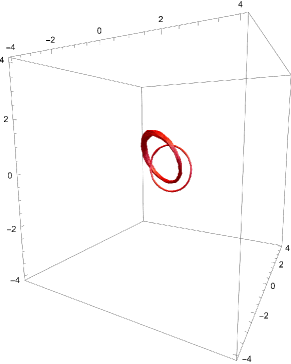
(a) $t=0$

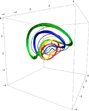
(b) $t/t_{0}=1/2$

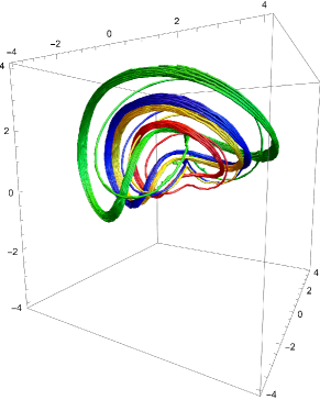
(c) $t/t_{0}=1$

Figure 1: Evolution of hopfion (5) of field lines ${\bf D}$ in different cosmological settings. (a) For $t=0$. (b) For $t/t_{0}=1/2$, flat spacetime hopfion (red), radiation-dominated hopfion (blue), matter-dominated hopfion (green), and dark-energy cosmological hopfion (yellow). (c) For $t/t_{0}=1$ (same colors).

In Fig. 1, we plot the field lines of the hopfion solution (5) for ${\bf D}$ for several cosmological models, in different coordinate times $t$ (all plot boxes have the same scales and orientations). The hopfion solution for $t=0$ (with $a=1$), Fig. 1(a), coincide for all cosmological models.

In Figs. 1(b), we plot the different evolution for different cosmological models for $t/t_{0}=1/2$. In red lines, we plot the flat spacetime solution for comparison. These coincide with known solutions besieris ; irvine . In blue lines is depicted the same hopfion solution for a radiation-dominated scenario, corresponding to $\tau/t_{0}=\sqrt{2}$. In green lines, the hopfion solution for a matter-dominated cosmological model, for $\tau/t_{0}=(27/2)^{1/3}$. Lastly, in yellow lines, we present the hopfion for dark energy cosmology, with $\tau/t_{0}=e-e^{1/2}$, where we have considered $H_{0}t_{0}=1$.

In Figs. 1(c), we plot the solution for coordinate time $t/t_{0}=1$. Red lines are the hopfion solution in flat spacetime. The hopfion solution in the radiation-dominated Universe, in blue lines, now is plotted for $\tau/t_{0}=2$. In green lines, the matter-dominated hopfion solution is obtained for $\tau/t_{0}=3$. Finally, the evolution in a dark-energy cosmology, in yellow lines, is shown for $\tau/t_{0}=e-1$, with $H_{0}t_{0}=1$.

Thereby, in Fig. 1, we can see how, for the same coordinate times, the hopfion evolves faster in a radiation-dominated Universe than in flat spacetime. Even faster evolution occurs for a matter-dominated Universe. also, in a dark-energy scenario, faster development occur for the hopfion solution, which depends on the value of $H_{0}$.

These different evolution (spreading) rates of the cosmological hopfions are related to the fact that any electromagnetic wavepacket spread with time. In the cosmological context, the spreading of the electromagnetic wavepacket can be calculated from iwoff ; iwoff2

$$\frac{d^{2}}{d\tau^{2}}\int d^{3}r\,\left(r-\langle r(\tau)\rangle\right)^{2}\textbf{\emph{F}}^{*}\cdot\textbf{\emph{F}}=2\int d^{3}r\,\textbf{\emph{F}}^{*}\cdot\textbf{\emph{F}}\,,$$ (8)

which can be proved directly from Eqs. (2) for the center of the momentum frame of the electromagnetic wavepacket iwoff ; lekner . This implies that the second conformal-time derivative of the spreading of an electromagnetic wavepacket is constant (proportional to its energy). Thus, the spreading of a cosmological electromagnetic hopfion is proportional to the square of conformal time, $\tau^{2}$. In terms of the coordinate time, this implies that hopfions spread at different rates depending on the cosmological setting in which they develops. This dependence is shown in Fig. 2, where we have plotted the square of the conformal time $\tau^{2}$ as a function of square of the proper time $t^{2}$. As expected, in flat spacetime $\tau^{2}=t^{2}$, which is shown as a straight red line. However, in any other cosmological scenario, the spreading is faster in terms of proper time. Besides, we show a shaded region that represents the different $\tau^{2}$ dependence in a perfect fluid cosmological setting, given by Eq. (6), for $0\leq w\leq 1$. For all these cases, the spreading is faster. In blue line, we present the spreading rate for a radiation-dominated scenario, and similarly, for a matter-dominated cosmology in green line. Lastly, in yellow line, we show the spreading time $\tau^{2}$ for a dark-energy cosmology for $H_{0}t_{0}=1$, and in yellow dashed-line for $H_{0}t_{0}=2$.

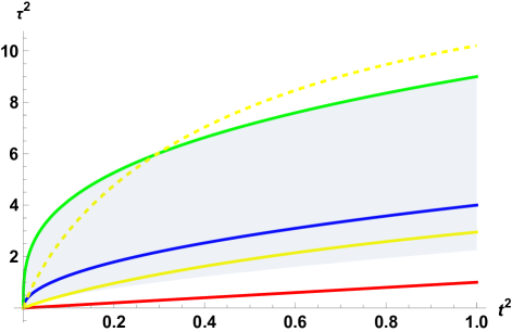
Figure 2: Cosmological time dependence of the electromagnetic wavepacket spreding with respect to its flat spacetime counterpart. Red line is for flat spacetime scenario. Blue and green lines are the faster spreading induced by the radiation-dominated and matter-dominated cosmologies, respectively. Yellow lines are for a Universe with dark energy content.

IV Remarks

All flat spacetime electromagnetic hopfions are also null electromagnetic solutions in FLRW cosmology. Although this is a simple consequence of the conformally flat nature of the FLRW metric, the evolution of the hopfion solution is different from the flat spacetime one, as the conformal time depends in a nonlinear way on the coordinate time.

In the above studied cosmological scenarios, hopfions disperse faster than their counterparts in flat spacetime. This can be seen in Fig. 1, where the hopfions disperse as they evolve and depart from its initial doughnut–like shape. However, a major general consequence of the cosmological evolution of any hopfion is the $\tau^{2}$-form of dispersion. This is valid for all cosmological electromagnetic solutions. Thus, any other solution for cosmological hopfions, it will have a faster dispersion $\tau^{2}>t^{2}$ (compared to flat spacetime ones) as long as $\tau>t$.

Nevertheless, this behavior is not valid for exotic forms of matter. For fluid with negative pressure (forms of dark energy), it is possible to have slower dispersion, such that $\tau^{2}<t^{2}$. Indeed, from Eq. (6) we find that this occur for equations of state $-1<w\leq-2/3$. These $w$ define a broad class of dark energy cosmologies without cosmological constant. The study of this class of cosmological electromagnetic hopfions is left for the future.

Finally, the presented solutions show the features that can be observed/measured in any cosmological hopfion. Also, they establish how cosmological hopfions can be modelled in laboratory using their flat spacetime analogues Jung-Shen ; particle .

- (1) H. Hopf, Mathematische Annalen, Berlin: Springer, 104, 637, (1931).
- (2) H. K. Urbantke, Journal of Geometry and Physics, 46, 125 (2003).
- (3) J.-S. B. Tai, P. J. Ackerman and I. I. Smalyukh, PNAS 115, 921 (2018).
- (4) D. Sugic, R. Droop, E. Otte et al., Nat. Commun. 12, 6785 (2021).
- (5) P. Ackerman, I. I. Smalyukh, Nature Mater. 16, 426 (2017)
- (6) B. G.-g. Chen et al., Phys. Rev. Lett. 110, 237801 (2013)
- (7) N. Kent, N. Reynolds, D. Raftrey et al., Nat. Commun. 12, 1562 (2021)
- (8) A. F. Rañada, Lett. Math. Phys., 18, 97 (1989).
- (9) A. F. Rañada, J. Phys. A: Math. Gen. 23 L815 (1990).
- (10) A. F. Rañada, J. Phys. A: Math. Gen. 25, 1621 (1992).
- (11) A. F. Rañada, and J. L. Trueba, Phys. Lett. A 202, 337 (1995).
- (12) A. F. Rañada, and J. L. Trueba, Phys. Lett. A 232, 25 (1997).
- (13) A. Grzela, J. Jezierski and T. Smołka, Acta Physica Polonica B Proceedings Supplement 16, 6-A17 (2023).
- (14) J. Plebanksi, Phys. Rev. 118, 1396 (1960).
- (15) F. de Felice, Gen. Relativ. Gravit. 2, 374 (1971).
- (16) B. Mashhoon, Phys. Rev. D 8, 4297 (1973).
- (17) B. Mashhoon, Phys. Rev. D 11, 2679 (1975).
- (18) F. A. Asenjo and S. A. Hojman, Phys. Rev. D 96, 044021 (2017).
- (19) I. M. Besieris and A. M. Shaarawi, Opt. Lett. 34, 3887 (2009).
- (20) W. Irvine and D. Bouwmeester, Nature Phys. 4, 716 (2008).
- (21) I. Bialynicki-Birula and Z. Bialynicka-Birula, Phys. Scr. 93, 104005 (2018).
- (22) M. Arrayás and J. L. Trueba, J. Phys. A: Math. Theor. 48, 025203 (2015).
- (23) A. Trautman, Int. J. Theo. Phys. 16, 561 (1977).
- (24) A. Thompson, A. Wickes, J. Swearngin and D. Bouwmeester, J. Phys. A: Math. Theor. 48, 205202 (2015).
- (25) W. T. M. Irvine, J. Phys. A: Math. Theor. 43, 385203 (2010).
- (26) C. Hoyos, N. Sircar and J. Sonnenschein, J. Phys. A: Math. Theor. 48, 255204 (2015).
- (27) B. Ryden, Introduction to Cosmology (Addison Wesley, San Francisco, 2003).
- (28) I. Bialynicki-Birula and Z. Bialynicka-Birula, J. Phys. A: Math. Theor. 46, 053001 (2013); 46 159501 (2013).
- (29) I. Bialynicki-Birula and Z. Bialynicka-Birula, Phys. Rev. A 100, 012108 (2019).
- (30) J. Lekner, J. Opt. A: Pure Appl. Opt. 6, 146 (2004).