Handbook of the analytic and expansion formulae for the muon $g-2$ anomaly

Abstract

Since announcement of the muon $g-2$ anomaly, plenty of papers have devoted to this anomaly. The approximate formulae are always adopted when determining the new physics contributions to $(g-2)_{\mu}$, while clear scope of applications are always absent. This manuscript is dedicated to the comprehensive analytical results and approximations for the canonical interactions at one-loop level, which can be a useful handbook for the model builders. Here, we only collect the analytic and approximate expressions for the scalar mediator case. For the expressions of vector mediator case, they will appear in the future.

I The introduction

The muon anomalous magnetic dipole moment (aMDM) is one of the crucial low energy observables sensitive to the new physics. It is marked as $a_{\mu}\equiv(g-2)/2$, where $g$ is the Lande factor. More introductions are reviewed in the articles [Miller:2007kk, Jegerlehner:2009ry, Jegerlehner:2017gek]. From the viewpoint of effective field theory, it corresponds to the dipole interaction $-\frac{ea_{\mu}}{4m_{\mu}}\bar{\mu}\sigma^{\mu\nu}\mu F_{\mu\nu}$. Here, $F_{\mu\nu}$ is the electromagnetic field tensor. In standard model (SM), the most precise prediction is calculated as $a_{\mu}^{\mathrm{SM}}=116591810(43)\times 10^{-11}$ from the 2020 white paper [Aoyama:2020ynm]. Its deviation from the standard model prediction can be the signal of new physics.

The muon $g-2$ anomaly was first reported by the E821 experiment at BNL [Muong-2:2006rrc]. In 2021, the FNAL muon $g-2$ experiment increased the tension between the SM prediction and experiment [Muong-2:2021ojo]. The average result is $a_{\mu}^{\mathrm{Exp}}=116592061(41)\times 10^{-11}$ after combining the BNL and FNAL Run-1 data, which shows the $4.2\sigma$ discrepancy between this average and the 2020 white paper prediction, namely $\Delta a_{\mu}\equiv a_{\mu}^{\mathrm{Exp}}-a_{\mu}^{\mathrm{SM}}=(251\pm 59)\times 10^{-11}$. Recently, the FNAL muon $g-2$ experiment has released the Run-2 and Run-3 data and it is consistent with the BNL and FNAL Run-1 data. The updated new world average is $a_{\mu}^{\mathrm{Exp}}=116592059(22)\times 10^{-11}$, which shows the $5.1\sigma$ deviation from the 2020 white paper prediction [Muong-2:2023cdq]. Although this anomaly can be caused by the experimental and theoretical uncertainties, we are interested in the contributions from new physics. There are many new physics models motivated to explain this anomaly [Jegerlehner:2009ry, Queiroz:2014zfa, Lindner:2016bgg], while the approximate formulae involved are not systematically investigated. In Ref.[Yu:2021suw], the authors studied several approximations. Hence, a comprehensive investigation of the relevant formulae is necessary, which is useful and convenient for the model builders. Here, we collect the analytic and approximate expressions for the scalar mediator case. The vector mediator case will appear in the updated version.

II The $(g-2)_{\mu}$ in simplified models

II.1 The simplified model

II.1.1 Canonical interactions

First, let us consider the muon interactions with a fermion and a scalar (vector) mediator. In special case, the fermion can also be muon. Then, the most general renormalizable Lagrangian can be written as

$$\mathcal{L}\supset\bar{\mu}(y_{S}+i\gamma^{5}y_{P})fS+\bar{\mu}\gamma^{\mu}(g_{V}+\gamma^{5}g_{A})fV_{\mu}+\mathrm{h.c.}~{}$$

$$=\bar{\mu}(y_{L}\omega_{-}+y_{R}\omega_{+})fS+\bar{\mu}\gamma^{\mu}(g_{L}\omega_{-}+g_{R}\omega_{+})fV_{\mu}+\mathrm{h.c.}~{},$$ (1)

where $\omega_{\pm}$ are the chirality projection operators $(1\pm\gamma^{5})/2$. The charge conservation requires $Q_{f}+Q_{S(V)}=-1$. Especially, $f$ is neutral for $Q_{S(V)}=-1$. On the contrary, $S(V)$ is neutral for $Q_{f}=-1$. Hereafter, the first line is named as $CP$ basis because of $CP$ even and odd interactions, and the second line is called as chiral basis because of the left-handed and right-handed interactions. The parameters in the two basis can be correlated through the relation

$$y_{S}=\frac{y_{L}+y_{R}}{2},y_{P}=\frac{y_{R}-y_{L}}{2i},g_{V}=\frac{g_{L}+g_{R}}{2},g_{A}=\frac{g_{R}-g_{L}}{2},$$ (2)

or equivalently,

$$y_{L}=y_{S}-iy_{P},y_{R}=y_{S}+iy_{P},g_{L}=g_{V}-g_{A},g_{R}=g_{V}+g_{A}.$$ (3)

Each basis has its own advantages and disadvantages. In the $CP$ basis, $CP$ even and odd contributions are separated, and there is no mixed contributions . Typically, $CP$ even and odd contributions have different sign. In the chiral basis, the chiral enhancement is explicitly isolated.

In the following, we present the corresponding quantum electrodynamics (QED) interactions

$$eQ_{f}\bar{f}\gamma^{\mu}fA_{\mu}+ieQ_{S}[S^{{\dagger}}(\partial^{\mu}S)-(\partial^{\mu}S)^{{\dagger}}S]A_{\mu}+ieQ_{V}\big{\{}[V_{\mu\nu}(V^{\mu})^{{\dagger}}-(V_{\mu\nu})^{{\dagger}}V^{\mu}]A^{\nu}+V_{\mu}(V_{\nu})^{{\dagger}}A^{\mu\nu}\big{\}},$$ (4)

where the $A_{\mu}$ labels the photon $\gamma$ and the $V_{\mu\nu}$ is defined as $(\partial_{\mu}V_{\nu}-\partial_{\nu}V_{\mu})$.

II.1.2 Comments on non-canonical interactions

In Eq. (II.1.1) and Eq. (4), the canonical interactions always appear in the renormalizable models, which are mainly investigated in this manuscript. Here are some comments on the more complex interactions:

1. The dimension six four-fermion (two muons and two fermions) interactions can also contribute to the $(g-2)_{\mu}$ if $f$ is charged. The results in the effective field theory framework are presented in Refs. [Jenkins:2013zja, Jenkins:2013wua, Alonso:2013hga, Jenkins:2017dyc, Aebischer:2021uvt].

2. The high dimensional operator can induce new $\mu fM$ interactions, for example, derivative interactions $\bar{\mu}\gamma^{\mu}f\partial_{\mu}S,\bar{\mu}\gamma^{\mu}\gamma^{5}f\partial_{\mu}S$ and dipole interactions $\bar{\mu}\sigma^{\mu\nu}fV_{\mu\nu},\bar{\mu}\sigma^{\mu\nu}\gamma^{5}fV_{\mu\nu}$ [Darme:2021qzw].

3. There can be non standard QED interactions.

   • $ff\gamma$ interaction: $\bar{f}\sigma^{\mu\nu}fA_{\mu\nu},\bar{f}\sigma^{\mu\nu}\gamma^{5}fA_{\mu\nu}$.

   • $SS\gamma$ interaction: $i[(\partial^{\mu}S)^{{\dagger}}(\partial^{\nu}S)-(\partial^{\nu}S)^{{\dagger}}(\partial^{\mu}S)]A_{\mu\nu}$.

   • $VV\gamma$ interaction:

     In general, the $WW\gamma$ interactions can be written as [Hagiwara:1993ck]

     $$ieQ_{W^{+}}[g_{\gamma}(W_{\mu\nu}^{+}W^{-,\mu}-W_{\mu\nu}^{-}W^{+,\mu})A^{\nu}+\kappa_{\gamma}W_{\mu}^{+}W_{\nu}^{-}A^{\mu\nu}+\frac{\lambda_{\gamma}}{m_{W}^{2}}W_{\mu\nu}^{+}W^{-,\nu\rho}A_{\rho}^{~{}\mu}].$$ (5)

     In the above, it returns to the SM for $g_{\gamma}=\kappa_{\gamma}=1$ and $\lambda_{\gamma}=0$. Similarly, the $VV\gamma$ interactions can also be modified when $W^{+}(W^{-})$ is replaced by $V(V^{{\dagger}})$. Their effects to $(g-2)_{\mu}$ are discussed in Ref. [Choudhury:2022iqz].

4. The fermion $f$ is usually spin half, while it can also be spin 3/2.

5. In addition to the scalar and vector mediators, the mediator can also be a graviton [Huang:2022zet].

6. exotic interactions: $SA_{\mu\nu}A^{\mu\nu},SA_{\mu\nu}Z^{\mu\nu}$.

II.2 The contributions

II.2.1 General structure of the one-loop contributions

The one-loop electro-weak corrections in the SM has been calculated in Ref. [Leveille:1977rc]. There are $W,Z,h$ contributions, of which the Higgs contribution is negligible because of the light muon Yukawa coupling.

In new physics models, there are two types of contributions. The first type originates from the modification of SM gauge interactions $Z\mu\mu,W\mu\nu_{\mu}$ and Yukawa interactions $h\mu\mu$. However, $Z\mu\mu,W\mu\nu_{\mu}$ couplings have been constrained strictly [Workman:2022ynf]. Although the deviation of SM $h\mu\mu$ coupling can be large [ATLAS:2020fzp, CMS:2020xwi], its contribution is suppressed by the small Yukawa coupling. The second type originates from the new scalar and vector mediated interactions. In fact, there are typically two types of Feynman diagrams at one-loop (see Fig. 1).

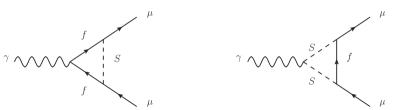
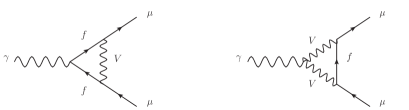
Figure 1: Typical scalar (upper) and vector (lower) mediator Feynman diagrams which contribute to the $(g-2)_{\mu}$.

Starting from the canonical interactions in Eq. (II.1.1) and Eq. (4), the new physics contributions to $(g-2)_{\mu}$ can be summed as [Leveille:1977rc]

$$\Delta a_{\mu}\equiv\Delta a_{\mu}^{S}+\Delta a_{\mu}^{V}=\frac{N_{C}m_{\mu}^{2}}{8\pi^{2}}\Bigg{[}\sum_{S}\frac{|y_{S}|^{2}(-Q_{f}I_{S}^{f}-Q_{S}I_{S}^{S})+|y_{P}|^{2}(-Q_{f}I_{P}^{f}-Q_{S}I_{P}^{S})}{m_{S}^{2}}$$

$$+\sum_{V}\frac{|g_{V}|^{2}(-Q_{f}L_{V}^{f}-Q_{V}L_{A}^{V})+|g_{A}|^{2}(-Q_{f}L_{V}^{f}-Q_{V}L_{A}^{V})}{m_{V}^{2}}\Bigg{]},$$ (6)

where the $\Delta a_{\mu}^{S}$ and $\Delta a_{\mu}^{V}$ label the contributions from the scalar and vector mediators. $N_{C}$ is the color factor. Hereafter, $I_{\times}^{f}$ and $L_{\times}^{f}$ mark the $ff\gamma$ vertex mediated loop functions. $I_{\times}^{S}$ and $L_{\times}^{V}$ mark the $SS\gamma$ and $VV\gamma$ vertex mediated loop functions. As we can see, contributions to $(g-2)_{\mu}$ are determined by the Yukawa (gauge) coupling, the scalar (vector) mediator mass, and the fermion mass.

In the chiral basis, it can also be expressed as

$$\Delta a_{\mu}=\frac{N_{C}m_{\mu}^{2}}{8\pi^{2}}\Bigg{\{}\sum_{S}\frac{(|y_{L}|^{2}+|y_{R}|^{2})(-Q_{f}I_{LL}^{f}-Q_{S}I_{LL}^{S})+\left[y_{L}(y_{R})^{\ast}+y_{R}(y_{L})^{\ast}\right](-Q_{f}I_{LR}^{f}-Q_{S}I_{LR}^{S})}{m_{S}^{2}}$$

$$+\sum_{V}\frac{(|g_{L}|^{2}+|g_{R}|^{2})(-Q_{f}L_{LL}^{f}-Q_{V}L_{LL}^{V})+\left[g_{L}(g_{R})^{\ast}+g_{R}(g_{L})^{\ast}\right](-Q_{f}L_{LR}^{f}-Q_{V}L_{LR}^{V})}{m_{V}^{2}}\Bigg{\}},$$ (7)

Using the relations in Eq. (2) and Eq. (3), we can derive the identities between the $CP$ and chiral basis integrals.

$$I_{S}^{f(S)}=2(I_{LL}^{f(S)}+I_{LR}^{f(S)}),I_{P}^{f(S)}=2(I_{LL}^{f(S)}-I_{LR}^{f(S)}),$$

$$L_{V}^{f(V)}=2(L_{LL}^{f(V)}+L_{LR}^{f(V)}),L_{A}^{f(V)}=2(L_{LL}^{f(V)}-L_{LR}^{f(V)}),$$ (8)

or equivalently,

$$I_{LL}^{f(S)}=\frac{I_{S}^{f(S)}+I_{P}^{f(S)}}{4},I_{LR}^{f(S)}=\frac{I_{S}^{f(S)}-I_{P}^{f(S)}}{4},$$

$$L_{LL}^{f(V)}=\frac{L_{V}^{f(V)}+L_{A}^{f(V)}}{4},L_{LR}^{f(V)}=\frac{L_{V}^{f(V)}-L_{A}^{f(V)}}{4},$$ (9)

II.2.2 Representations of loop functions

After integrating out the loop particles, we can obtain the results of loop functions $I_{\times}^{f(S)}$ and $L_{\times}^{f(V)}$, which can exhibit in different forms. Here, we impose three definitions of the loop function representations.

• PaVe representation
  The loop functions are expressed in terms of the Passarino-Veltman integrals, namely, the $\mathbf{A},\mathbf{B},\mathbf{C},\mathbf{D}$ functions.

• Integral representation
  The loop functions are expressed in terms of the integrals.

• Special function representation
  The loop functions are expressed in terms of pre-defined functions. Although the $C_{0}$ function will be expressed in di-logarithm forms under nomal circumstances, it can be simplified because of the zero momentum square of the photon and two same internal propagator masses. Now, let us define the following function:

  $$f(k^{2},m_{0}^{2},m_{1}^{2})\equiv\lim_{\epsilon\rightarrow 0^{+}}\int_{0}^{1}dx\frac{1}{xm_{0}^{2}+(1-x)m_{1}^{2}-x(1-x)k^{2}-i\epsilon}$$

  $$=\left\{\begin{array}[]{ll}\frac{1}{\sqrt{\Delta}}(\log\frac{m_{0}^{2}+m_{1}^{2}-k^{2}+\sqrt{\Delta}}{m_{0}^{2}+m_{1}^{2}-k^{2}-\sqrt{\Delta}}+2i\pi)&,\quad\textrm{for}\quad k^{2}>(m_{0}+m_{1})^{2}\\ \frac{1}{\sqrt{\Delta}}\log\frac{m_{0}^{2}+m_{1}^{2}-k^{2}+\sqrt{\Delta}}{m_{0}^{2}+m_{1}^{2}-k^{2}-\sqrt{\Delta}}&,\quad\textrm{for}\quad 0<k^{2}<(m_{0}-m_{1})^{2}\\ \frac{2}{\sqrt{-\Delta}}\arctan\frac{\sqrt{-\Delta}}{m_{0}^{2}+m_{1}^{2}-k^{2}}&,\quad\textrm{for}\quad(m_{0}-m_{1})^{2}<k^{2}<(m_{0}+m_{1})^{2}\\ \frac{1}{m_{0}m_{1}}&,\quad\textrm{for}\quad k^{2}=(m_{0}-m_{1})^{2}\\ -\frac{1}{m_{0}m_{1}}&,\quad\textrm{for}\quad k^{2}=(m_{0}+m_{1})^{2}\\ \frac{1}{m_{0}^{2}-m_{1}^{2}}\log\frac{m_{0}^{2}}{m_{1}^{2}}&,\quad\textrm{for}\quad k^{2}=0\end{array}\right..$$ (16)

  Here, $\Delta=k^{4}+m_{0}^{4}+m_{1}^{4}-2(k^{2}m_{0}^{2}+k^{2}m_{1}^{2}+m_{0}^{2}m_{1}^{2})$. This function agrees with the function defined in Ref. [Albergaria:2022jne]. According to the definition, we have the property $f(k^{2},m_{0}^{2},m_{1}^{2})=f(k^{2},m_{1}^{2},m_{0}^{2})$.

II.2.3 Explicit form of the loop functions in different representations: scalar mediator case

In this section, we show the explicit form of the loop functions in the PaVe representation, Integral representation, and Special function representation. For simplicity, we drop the $-i\epsilon$ in the Integral representation, which should be remembered when encountering the branch cut. Let us introduce two dimensionless parameters $\lambda_{i}\equiv\frac{m_{\mu}}{m_{i}}$ and $\epsilon_{f}\equiv\frac{m_{f}}{m_{\mu}}$. Here, $m_{i}$ labels the scalar or vector mediator mass and $m_{f}$ labels the fermion $f$ mass. Then, the $I_{LL}^{f}$ is computed as

$$I_{LL}^{f}(m_{f},m_{S})=m_{S}^{2}[C_{11}(m_{\mu}^{2},0,m_{\mu}^{2},m_{S}^{2},m_{f}^{2},m_{f}^{2})+C_{12}(m_{\mu}^{2},0,m_{\mu}^{2},m_{S}^{2},m_{f}^{2},m_{f}^{2})+C_{1}(m_{\mu}^{2},0,m_{\mu}^{2},m_{S}^{2},m_{f}^{2},m_{f}^{2})]$$

$$=\frac{m_{S}^{2}}{16m_{\mu}^{4}}[(3m_{S}^{2}+m_{\mu}^{2}-5m_{f}^{2})B_{0}(0,m_{f}^{2},m_{f}^{2})+2m_{S}^{2}B_{0}(0,m_{S}^{2},m_{S}^{2})+(5m_{f}^{2}-m_{\mu}^{2}-5m_{S}^{2})B_{0}(m_{\mu}^{2},m_{f}^{2},m_{S}^{2})$$

$$+(3m_{S}^{4}-2m_{S}^{2}m_{\mu}^{2}-6m_{S}^{2}m_{f}^{2}+3m_{f}^{4}-2m_{f}^{2}m_{\mu}^{2}-m_{\mu}^{4})C_{0}(m_{\mu}^{2},0,m_{\mu}^{2},m_{S}^{2},m_{f}^{2},m_{f}^{2})+2(m_{S}^{2}-m_{\mu}^{2}-m_{f}^{2})]$$

$$=\frac{1}{2}\int_{0}^{1}dx\frac{x^{2}(1-x)m_{S}^{2}}{(1-x)m_{S}^{2}-x(1-x)m_{\mu}^{2}+xm_{f}^{2}}=\frac{1}{2}\int_{0}^{1}dx\frac{x^{2}(1-x)}{(1-x)(1-\lambda_{S}^{2}x)+\epsilon_{f}^{2}\lambda_{S}^{2}x}$$

$$=\frac{m_{S}^{2}}{4m_{\mu}^{6}}\Big{\{}[m_{f}^{6}-(3m_{S}^{2}+2m_{\mu}^{2})m_{f}^{4}+(3m_{S}^{4}+m_{S}^{2}m_{\mu}^{2}+m_{\mu}^{4})m_{f}^{2}+m_{S}^{4}m_{\mu}^{2}-m_{S}^{6}]f(m_{\mu}^{2},m_{f}^{2},m_{S}^{2})$$

$$+[-m_{f}^{4}+(2m_{S}^{2}+m_{\mu}^{2})m_{f}^{2}-m_{S}^{4}]\log\frac{m_{f}^{2}}{m_{S}^{2}}+m_{\mu}^{2}(2m_{f}^{2}-2m_{S}^{2}-m_{\mu}^{2})\Big{\}}.$$ (17)

The $I_{LR}^{f}$ is computed as

$$I_{LR}^{f}(m_{f},m_{S})=\epsilon_{f}m_{S}^{2}C_{1}(m_{\mu}^{2},0,m_{\mu}^{2},m_{S}^{2},m_{f}^{2},m_{f}^{2})$$

$$=\frac{m_{f}m_{S}^{2}}{4m_{\mu}^{3}}[B_{0}(m_{\mu}^{2},m_{f}^{2},m_{S}^{2})-B_{0}(0,m_{f}^{2},m_{f}^{2})+(m_{f}^{2}-m_{S}^{2}-m_{\mu}^{2})C_{0}(m_{\mu}^{2},0,m_{\mu}^{2},m_{S}^{2},m_{f}^{2},m_{f}^{2})]$$

$$=\frac{m_{f}}{2m_{\mu}}\int_{0}^{1}dx\frac{x^{2}m_{S}^{2}}{(1-x)m_{S}^{2}-x(1-x)m_{\mu}^{2}+xm_{f}^{2}}=\frac{\epsilon_{f}}{2}\int_{0}^{1}dx\frac{x^{2}}{(1-x)(1-\lambda_{S}^{2}x)+\epsilon_{f}^{2}\lambda_{S}^{2}x}$$

$$=\frac{m_{f}m_{S}^{2}}{4m_{\mu}^{5}}\Big{\{}[m_{f}^{4}-2m_{f}^{2}(m_{S}^{2}+m_{\mu}^{2})+m_{S}^{4}+m_{\mu}^{4}]f(m_{\mu}^{2},m_{f}^{2},m_{S}^{2})$$

$$+(m_{S}^{2}+m_{\mu}^{2}-m_{f}^{2})\log\frac{m_{f}^{2}}{m_{S}^{2}}+2m_{\mu}^{2}\Big{\}}.$$ (18)

The $I_{LL}^{S}$ is computed as

$$I_{LL}^{S}(m_{f},m_{S})=-\frac{1}{2}m_{S}^{2}[C_{11}(m_{\mu}^{2},m_{\mu}^{2},0,m_{S}^{2},m_{f}^{2},m_{S}^{2})+C_{1}(m_{\mu}^{2},m_{\mu}^{2},0,m_{S}^{2},m_{f}^{2},m_{S}^{2})]$$

$$=\frac{m_{S}^{2}}{16m_{\mu}^{4}}[(5m_{S}^{2}-m_{\mu}^{2}-3m_{f}^{2})B_{0}(0,m_{S}^{2},m_{S}^{2})-2m_{f}^{2}B_{0}(0,m_{f}^{2},m_{f}^{2})+(5m_{f}^{2}+m_{\mu}^{2}-5m_{S}^{2})B_{0}(m_{\mu}^{2},m_{f}^{2},m_{S}^{2})$$

$$+(-3m_{S}^{4}+2m_{S}^{2}m_{\mu}^{2}+6m_{S}^{2}m_{f}^{2}-3m_{f}^{4}+2m_{f}^{2}m_{\mu}^{2}+m_{\mu}^{4})C_{0}(m_{\mu}^{2},0,m_{\mu}^{2},m_{f}^{2},m_{S}^{2},m_{S}^{2})+2(m_{S}^{2}+m_{\mu}^{2}-m_{f}^{2})]$$

$$=-\frac{1}{2}\int_{0}^{1}dx\frac{x(1-x)^{2}m_{S}^{2}}{(1-x)m_{S}^{2}-x(1-x)m_{\mu}^{2}+xm_{f}^{2}}=-\frac{1}{2}\int_{0}^{1}dx\frac{x(1-x)^{2}}{(1-x)(1-\lambda_{S}^{2}x)+\epsilon_{f}^{2}\lambda_{S}^{2}x}$$

$$=\frac{m_{S}^{2}}{4m_{\mu}^{6}}\Big{\{}[m_{f}^{6}-(3m_{S}^{2}+m_{\mu}^{2})m_{f}^{4}+(3m_{S}^{2}-m_{\mu}^{2})m_{S}^{2}m_{f}^{2}-m_{S}^{2}(m_{\mu}^{2}-m_{S}^{2})^{2}]f(m_{\mu}^{2},m_{f}^{2},m_{S}^{2})$$

$$+[-m_{f}^{4}+2m_{S}^{2}m_{f}^{2}+m_{S}^{2}m_{\mu}^{2}-m_{S}^{4}]\log\frac{m_{f}^{2}}{m_{S}^{2}}+m_{\mu}^{2}(2m_{f}^{2}-2m_{S}^{2}+m_{\mu}^{2})\Big{\}}.$$ (19)

The $I_{LR}^{S}$ is computed as

$$I_{LR}^{S}(m_{f},m_{S})=-\frac{m_{f}}{2m_{\mu}}m_{S}^{2}C_{1}(m_{\mu}^{2},m_{\mu}^{2},0,m_{S}^{2},m_{f}^{2},m_{S}^{2})$$

$$=\frac{m_{f}m_{S}^{2}}{4m_{\mu}^{3}}[B_{0}(m_{\mu}^{2},m_{f}^{2},m_{S}^{2})-B_{0}(0,m_{S}^{2},m_{S}^{2})+(m_{S}^{2}+m_{\mu}^{2}-m_{f}^{2})C_{0}(m_{\mu}^{2},m_{\mu}^{2},0,m_{S}^{2},m_{f}^{2},m_{S}^{2})]$$

$$=-\frac{m_{f}}{2m_{\mu}}\int_{0}^{1}dx\frac{x(1-x)m_{S}^{2}}{(1-x)m_{S}^{2}-x(1-x)m_{\mu}^{2}+xm_{f}^{2}}=-\frac{\epsilon_{f}}{2}\int_{0}^{1}dx\frac{x(1-x)}{(1-x)(1-\lambda_{S}^{2}x)+\epsilon_{f}^{2}\lambda_{S}^{2}x}$$

$$=\frac{m_{f}m_{S}^{2}}{4m_{\mu}^{5}}\Big{\{}[m_{f}^{4}-m_{f}^{2}(2m_{S}^{2}+m_{\mu}^{2})+m_{S}^{4}-m_{S}^{2}m_{\mu}^{2}]f(m_{\mu}^{2},m_{f}^{2},m_{S}^{2})$$

$$+(m_{S}^{2}-m_{f}^{2})\log\frac{m_{f}^{2}}{m_{S}^{2}}+2m_{\mu}^{2}\Big{\}}.$$ (20)

In fact, the $I_{LR}^{f}$ can be correlated with $I_{LL}^{f}$ through the following relation:

$$I_{LR}^{f}(m_{f},m_{S})=\frac{m_{f}}{4m_{\mu}}\cdot$$

$$\frac{4m_{\mu}^{2}[(m_{f}^{2}-m_{S}^{2}-m_{\mu}^{2})^{2}-2m_{S}^{2}m_{\mu}^{2}]I_{LL}^{f}(m_{f},m_{S})+m_{S}^{2}[m_{f}^{4}-2m_{f}^{2}(2m_{S}^{2}+m_{\mu}^{2})+3m_{S}^{4}+2m_{S}^{2}m_{\mu}^{2}+m_{\mu}^{4}+2m_{S}^{4}\log\frac{m_{f}^{2}}{m_{S}^{2}}]}{m_{f}^{6}-m_{f}^{4}(3m_{S}^{2}+2m_{\mu}^{2})+m_{f}^{2}(3m_{S}^{4}+m_{S}^{2}m_{\mu}^{2}+m_{\mu}^{4})+m_{S}^{4}m_{\mu}^{2}-m_{S}^{6}}.$$

Moreover, the $I_{LL}^{S}$ and $I_{LR}^{S}$ can be obtained via the following replacements:

$$I_{LL}^{S}(m_{f},m_{S})=-\frac{m_{S}^{2}}{m_{f}^{2}}\cdot I_{LL}^{f}(m_{S},m_{f}),$$

$$I_{LR}^{S}(m_{f},m_{S})=-\frac{m_{S}^{2}}{m_{f}m_{\mu}}\cdot I_{LL}^{f}(m_{S},m_{f})-\frac{m_{f}}{m_{\mu}}\cdot I_{LL}^{f}(m_{f},m_{S}).$$ (22)

II.2.4 Explicit form of the loop functions in different representations: vector mediator case

This section will be finished in the updated version.

II.2.5 Properties of the $f(k^{2},m_{0}^{2},m_{1}^{2})$ function

As we have shown in Sec. II.2.3, all the loop functions can be expressed as $f$ function in the Special function representation. Hence, it is of great importance to study the analytic and asymptotic behaviours of the function $f$, which is the task of this section.

1. Analytic Properties
   In general, we can treat $f$ as a complex function with three complex variables. In the three dimensional complex space, there is a branch cut for $k^{2}=(m_{0}+m_{1})^{2}$. This is consistent with the facts that the imaginary (absorptive) parts of $I_{LL(LR)}^{f(S)}$ and $L_{LL(LR)}^{f(V)}$ can appear in the case of $m_{\mu}>m_{f}+m_{S}$ (The loop particles can be on-shell.).

   Furthermore, $m_{0}=0$ and $m_{1}=0$ are the singular points, because we have the following identity:

   $$\frac{1}{\sqrt{\Delta}}\log\frac{m_{0}^{2}+m_{1}^{2}-k^{2}+\sqrt{\Delta}}{m_{0}^{2}+m_{1}^{2}-k^{2}-\sqrt{\Delta}}=\frac{1}{\sqrt{\Delta}}\log\frac{(m_{0}^{2}+m_{1}^{2}-k^{2}+\sqrt{\Delta})^{2}}{4m_{0}^{2}m_{1}^{2}}$$ (23)

2. Symmetric Properties $f(k^{2},m_{0}^{2},m_{1}^{2})=f(k^{2},m_{1}^{2},m_{0}^{2})$.

3. Asymptotic Properties

   • Expansion at $k^{2}=0$:

     $$f(k^{2},m_{0}^{2},m_{1}^{2})=\left\{\begin{array}[]{ll}\frac{1}{m_{0}^{2}-m_{1}^{2}}\log\frac{m_{0}^{2}}{m_{1}^{2}}+\frac{(m_{0}^{2}+m_{1}^{2})\log\frac{m_{0}^{2}}{m_{1}^{2}}-2(m_{0}^{2}-m_{1}^{2})}{(m_{0}^{2}-m_{1}^{2})^{3}}k^{2}\\ +\frac{(m_{0}^{4}+4m_{0}^{2}m_{1}^{2}+m_{1}^{4})\log\frac{m_{0}^{2}}{m_{1}^{2}}-3(m_{0}^{4}-m_{1}^{4})}{(m_{0}^{2}-m_{1}^{2})^{5}}k^{4}+\mathcal{O}(k^{6})&,\quad\textrm{for}\quad m_{0}\neq m_{1}\\ \\ \frac{1}{m_{0}^{2}}(1+\frac{k^{2}}{6m_{0}^{2}}+\frac{k^{4}}{30m_{0}^{4}})+\mathcal{O}(k^{6})&,\quad\textrm{for}\quad m_{0}=m_{1}\end{array}\right..$$ (28)

   • Expansion at $k^{2}\rightarrow\infty$:

     $$f(k^{2},m_{0}^{2},m_{1}^{2})=\frac{2}{k^{2}}\big{[}1+\frac{m_{0}^{2}+m_{1}^{2}}{k^{2}}+\frac{m_{0}^{4}+4m_{0}^{2}m_{1}^{2}+m_{1}^{4}}{k^{4}}\big{]}(-\log\frac{k^{2}}{m_{0}m_{1}}+i\pi)$$

     $$+\frac{2(m_{0}^{2}+m_{1}^{2})}{k^{4}}+\frac{3m_{0}^{4}+8m_{0}^{2}m_{1}^{2}+3m_{1}^{4}}{k^{6}}+\mathcal{O}(\frac{1}{k^{8}}).$$ (29)

   • Expansion at $m_{0}=0$:

     $$f(k^{2},m_{0}^{2},m_{1}^{2})$$

     $$=\left\{\begin{array}[]{ll}\frac{1}{m_{1}^{2}-k^{2}}\big{[}1+\frac{k^{2}+m_{1}^{2}}{(k^{2}-m_{1}^{2})^{2}}m_{0}^{2}+\frac{k^{4}+4k^{2}m_{1}^{2}+m_{1}^{4}}{(k^{2}-m_{1}^{2})^{4}}m_{0}^{4}\big{]}\cdot\big{[}\log\frac{(m_{1}^{2}-k^{2})^{2}}{m_{0}^{2}m_{1}^{2}}-2i\pi\theta(k^{2}-m_{1}^{2})\big{]}\\ +\frac{2k^{2}}{(k^{2}-m_{1}^{2})^{3}}m_{0}^{2}+\frac{k^{2}(3k^{2}+4m_{1}^{2})}{(k^{2}-m_{1}^{2})^{5}}m_{0}^{4}+\mathcal{O}(m_{0}^{6})\qquad\qquad\qquad\qquad\qquad\qquad,\textrm{for}\quad k^{2}\neq m_{1}^{2}\\ \\ \frac{\pi}{2\sqrt{m_{0}^{2}k^{2}}}(1+\frac{m_{0}^{2}}{8k^{2}}+\frac{3m_{0}^{4}}{128k^{4}}+\frac{5m_{0}^{6}}{1024k^{6}})-\frac{1}{2k^{2}}(1+\frac{m_{0}^{2}}{6k^{2}}+\frac{m_{0}^{4}}{30k^{4}})+\mathcal{O}(m_{0}^{6})\quad,\textrm{for}\quad k^{2}=m_{1}^{2}\end{array}\right..$$ (34)

     In the above, $\theta(x)$ is the Heaviside step function, which is defined as $\theta(x)=1$ for $x>0$ and $\theta(x)=0$ for $x<0$. We can find that $f(k^{2},m_{0}^{2},m_{1}^{2})$ diverges for $m_{0}\rightarrow 0$, which can lead to the infrared divergence.

   • Expansion at $m_{0}\rightarrow\infty$:

     $$f(k^{2},m_{0}^{2},m_{1}^{2})=\frac{1}{m_{0}^{2}}\log\frac{m_{0}^{2}}{m_{1}^{2}}+\big{[}(k^{2}+m_{1}^{2})\log\frac{m_{0}^{2}}{m_{1}^{2}}-2k^{2}\big{]}\frac{1}{m_{0}^{4}}$$

     $$+\big{[}(k^{4}+4k^{2}m_{1}^{2}+m_{1}^{4})\log\frac{m_{0}^{2}}{m_{1}^{2}}-k^{2}(3k^{2}+4m_{1}^{2})\big{]}\frac{1}{m_{0}^{6}}+\mathcal{O}(\frac{1}{m_{0}^{8}}).$$ (35)

   • For expansion at $m_{1}=0$ and $m_{1}\rightarrow\infty$, the results can be obtained through the replacement of $m_{0}\leftrightarrow m_{1}$ in Eq. (• ‣ \arabicenumi⃝) and Eq. (• ‣ \arabicenumi⃝).

4. Degenerate mass Properties
   

   • Case of $m_{0}^{2}=m_{1}^{2}\equiv m^{2}$:
     $f(k^{2},m^{2},m^{2})$ can be reduced as

     $$f(k^{2},m^{2},m^{2})=\left\{\begin{array}[]{ll}\frac{1}{\sqrt{k^{4}-4m^{2}k^{2}}}(\log\frac{2m^{2}-k^{2}+\sqrt{k^{4}-4m^{2}k^{2}}}{2m^{2}-k^{2}-\sqrt{k^{4}-4m^{2}k^{2}}}+2i\pi)&,\quad\textrm{for}\quad k^{2}>4m^{2}\\ \frac{2}{\sqrt{4m^{2}k^{2}-k^{4}}}\arctan\frac{\sqrt{4m^{2}k^{2}-k^{4}}}{2m^{2}-k^{2}}&,\quad\textrm{for}\quad 0<k^{2}<4m^{2}\\ \frac{1}{m^{2}}&,\quad\textrm{for}\quad k^{2}=0\\ -\frac{1}{m^{2}}&,\quad\textrm{for}\quad k^{2}=4m^{2}\end{array}\right..$$ (40)

     Then, they can be expanded as

     $$f(k^{2},m^{2},m^{2})=\left\{\begin{array}[]{ll}\frac{2}{k^{2}}\big{[}(1+\frac{2m^{2}}{k^{2}}+\frac{6m^{4}}{k^{4}})(-\log\frac{k^{2}}{m^{2}}+i\pi)+\frac{2m^{2}}{k^{2}}+\frac{7m^{4}}{k^{4}}+\mathcal{O}(\frac{m^{6}}{k^{6}})\big{]}&,\;\textrm{for}\;k^{2}\gg m^{2}\\ \\ \frac{1}{m^{2}}\big{[}1+\frac{k^{2}}{6m^{2}}+\frac{k^{4}}{30m^{4}}+\mathcal{O}(\frac{k^{6}}{m^{6}})\big{]}&,\;\textrm{for}\;k^{2}\ll m^{2}\end{array}\right..$$ (44)

   • Case of $k^{2}=m_{0}^{2}$:
     $f(m_{0}^{2},m_{0}^{2},m_{1}^{2})$ can be reduced as

     $$f(m_{0}^{2},m_{0}^{2},m_{1}^{2})=\left\{\begin{array}[]{ll}\frac{1}{m_{1}\sqrt{m_{1}^{2}-4m_{0}^{2}}}\log\frac{m_{1}+\sqrt{m_{1}^{2}-4m_{0}^{2}}}{m_{1}-\sqrt{m_{1}^{2}-4m_{0}^{2}}}&,\quad\textrm{for}\quad m_{1}>2m_{0}\\ \frac{2}{m_{1}\sqrt{4m_{0}^{2}-m_{1}^{2}}}\arctan\frac{\sqrt{4m_{0}^{2}-m_{1}^{2}}}{m_{1}}&,\quad\textrm{for}\quad m_{1}<2m_{0}\\ \frac{1}{m_{0}m_{1}}&,\quad\textrm{for}\quad m_{1}=2m_{0}\end{array}\right..$$ (48)

     Then, they can be expanded as

     $$f(m_{0}^{2},m_{0}^{2},m_{1}^{2})$$

     $$=\left\{\begin{array}[]{ll}\frac{2}{m_{1}^{2}}\big{[}(1+\frac{2m_{0}^{2}}{m_{1}^{2}}+\frac{6m_{0}^{4}}{m_{1}^{4}})\log\frac{m_{1}}{m_{0}}-\frac{m_{0}^{2}}{m_{1}^{2}}-\frac{7m_{0}^{4}}{2m_{1}^{4}}+\mathcal{O}(\frac{m_{0}^{6}}{m_{1}^{6}})\big{]}&,\;\textrm{for}\;m_{1}\gg m_{0}\\ \\ -\frac{1}{2m_{0}^{2}}\big{[}1+\frac{m_{1}^{2}}{6m_{0}^{2}}+\frac{m_{1}^{4}}{30m_{0}^{4}}+\mathcal{O}(\frac{m_{1}^{6}}{m_{0}^{6}})\big{]}+\frac{\pi}{2m_{0}m_{1}}\big{[}1+\frac{m_{1}^{2}}{8m_{0}^{2}}+\frac{3m_{1}^{4}}{128m_{0}^{4}}+\mathcal{O}(\frac{m_{1}^{6}}{m_{0}^{6}})\big{]}&,\;\textrm{for}\;m_{1}\ll m_{0}\end{array}\right..$$ (52)

   • Case of $k^{2}=m_{1}^{2}$:
     This case can be reduced into the case of $k^{2}=m_{0}^{2}$ owing to the symmetric properties, namely, $f(m_{1}^{2},m_{0}^{2},m_{1}^{2})=f(m_{1}^{2},m_{1}^{2},m_{0}^{2})$.

   • Case of $k^{2}=m_{0}^{2}=m_{1}^{2}$:
     In this case, we have $f(k^{2},k^{2},k^{2})=\frac{2\pi}{3\sqrt{3}k^{2}}$.

III Expansion of the loop functions

There are two methods to obtain the expansion results of the loop functions. One method is to start from the Integral representation in Sec. II.2.3 and Sec. II.2.4. The other method is to start from the Special function representation in Sec. II.2.3 and Sec. II.2.4, in which the expansions of $f$ function have been given in Sec. II.2.5.

III.1 Hierarchical mass expansion for the $I_{LL}^{f}$ and $I_{LR}^{f}$

III.1.1 Scenario of $m_{\mu}\ll m_{f},m_{S}$

The integrals $I_{LL}^{f}$ and $I_{LR}^{f}$ can be expanded as

$$I_{LL}^{f}=\frac{m_{S}^{2}(2m_{S}^{6}+3m_{S}^{4}m_{f}^{2}-6m_{S}^{2}m_{f}^{4}+m_{f}^{6}+12m_{S}^{4}m_{f}^{2}\log\frac{m_{f}}{m_{S}})}{12(m_{S}^{2}-m_{f}^{2})^{4}}+\mathcal{O}(m_{\mu}^{2})$$ (53)

and

$$I_{LR}^{f}=\frac{m_{f}m_{S}^{2}(-3m_{S}^{4}+4m_{S}^{2}m_{f}^{2}-m_{f}^{4}-4m_{S}^{4}\log\frac{m_{f}}{m_{S}})}{4m_{\mu}(m_{S}^{2}-m_{f}^{2})^{3}}+\mathcal{O}(m_{\mu}).$$ (54)

This coincides with those results in the supersymmetry models [Moroi:1995yh, Martin:2001st, Stockinger:2006zn] .

Especially, we have the following approximations:

$$I_{LL}^{f}\approx\left\{\begin{array}[]{ll}\frac{1}{6}(1+\frac{11m_{f}^{2}}{2m_{S}^{2}}-\frac{6m_{f}^{2}}{m_{S}^{2}}\log\frac{m_{S}}{m_{f}}),&\mathrm{for}~{}m_{\mu}\ll m_{f}\ll m_{S}\\ \frac{m_{S}^{2}}{12m_{f}^{2}}(1-\frac{2m_{S}^{2}}{m_{f}^{2}}),&\mathrm{for}~{}m_{\mu}\ll m_{S}\ll m_{f}\\ \frac{1}{24},&\mathrm{for}~{}m_{\mu}\ll m_{f}=m_{S}\end{array}\right.$$ (58)

and

$$I_{LR}^{f}\approx\left\{\begin{array}[]{ll}\frac{m_{f}}{m_{\mu}}\Big{[}\log\frac{m_{S}}{m_{f}}-\frac{3}{4}+\frac{m_{f}^{2}}{m_{S}^{2}}(3\log\frac{m_{S}}{m_{f}}-\frac{5}{4})\Big{]},&\mathrm{for}~{}m_{\mu}\ll m_{f}\ll m_{S}\\ \frac{m_{S}^{2}}{4m_{f}m_{\mu}}(1-\frac{m_{S}^{2}}{m_{f}^{2}}),&\mathrm{for}~{}m_{\mu}\ll m_{S}\ll m_{f}\\ \frac{m_{f}}{6m_{\mu}},&\mathrm{for}~{}m_{\mu}\ll m_{f}=m_{S}\end{array}\right..$$ (62)

III.1.2 Scenario of $m_{S}\ll m_{f},m_{\mu}$

The integrals $I_{LL}^{f}$ and $I_{LR}^{f}$ can be expanded as

$$I_{LL}^{f}=\left\{\begin{array}[]{ll}\frac{m_{S}^{2}}{4m_{\mu}^{6}}(1+\frac{2m_{S}^{2}}{m_{\mu}^{2}-m_{f}^{2}})\big{[}2m_{f}^{2}m_{\mu}^{2}-m_{\mu}^{4}+2m_{f}^{2}(m_{f}^{2}-m_{\mu}^{2})\log(1-\frac{m_{\mu}^{2}}{m_{f}^{2}})\big{]}+\mathcal{O}(m_{S}^{6}),&\mathrm{for}~{}m_{\mu}<m_{f}\\ \frac{m_{S}^{2}}{4m_{\mu}^{6}}(1+\frac{2m_{S}^{2}}{m_{\mu}^{2}-m_{f}^{2}})\big{[}2m_{f}^{2}m_{\mu}^{2}-m_{\mu}^{4}+2m_{f}^{2}(m_{f}^{2}-m_{\mu}^{2})(\log\frac{m_{\mu}^{2}-m_{f}^{2}}{m_{f}^{2}}-i\pi)\big{]}+\mathcal{O}(m_{S}^{6}),&\mathrm{for}~{}m_{\mu}>m_{f}\end{array}\right.$$ (65)

and

$$I_{LR}^{f}=\left\{\begin{array}[]{ll}\frac{m_{S}^{2}m_{f}}{2m_{\mu}^{3}}(1+\frac{m_{S}^{2}}{m_{\mu}^{2}-m_{f}^{2}})\big{[}1+(\frac{m_{f}^{2}}{m_{\mu}^{2}}-1)\log(1-\frac{m_{\mu}^{2}}{m_{f}^{2}})\big{]}+\mathcal{O}(m_{S}^{6}),&\mathrm{for}~{}m_{\mu}<m_{f}\\ \frac{m_{S}^{2}m_{f}}{2m_{\mu}^{3}}(1+\frac{m_{S}^{2}}{m_{\mu}^{2}-m_{f}^{2}})\big{[}1+(\frac{m_{f}^{2}}{m_{\mu}^{2}}-1)(\log\frac{m_{\mu}^{2}-m_{f}^{2}}{m_{f}^{2}}-i\pi)\big{]}+\mathcal{O}(m_{S}^{6}),&\mathrm{for}~{}m_{\mu}>m_{f}\\ \end{array}\right..$$ (68)

Especially, we have the following approximations:

$$I_{LL}^{f}\approx\left\{\begin{array}[]{ll}-\frac{m_{S}^{2}}{4m_{\mu}^{2}}\big{[}1-\frac{2m_{f}^{2}}{m_{\mu}^{2}}(1-\log\frac{m_{\mu}^{2}}{m_{f}^{2}}+i\pi)\big{]},&\mathrm{for}~{}m_{S}\ll m_{f}\ll m_{\mu}\\ \frac{m_{S}^{2}}{12m_{f}^{2}}(1+\frac{m_{\mu}^{2}}{2m_{f}^{2}}),&\mathrm{for}~{}m_{S}\ll m_{\mu}\ll m_{f}\\ \frac{m_{S}^{2}}{4m_{\mu}^{2}},&\mathrm{for}~{}m_{S}\ll m_{f}=m_{\mu}\end{array}\right.$$ (72)

and

$$I_{LR}^{f}\approx\left\{\begin{array}[]{ll}\frac{m_{S}^{2}m_{f}}{2m_{\mu}^{3}}\big{[}1-\log\frac{m_{\mu}^{2}}{m_{f}^{2}}+i\pi+\frac{m_{f}^{2}}{m_{\mu}^{2}}(1+\log\frac{m_{\mu}^{2}}{m_{f}^{2}}-i\pi)\big{]},&\mathrm{for}~{}m_{S}\ll m_{f}\ll m_{\mu}\\ \frac{m_{S}^{2}}{4m_{f}m_{\mu}}(1+\frac{m_{\mu}^{2}}{3m_{f}^{2}}),&\mathrm{for}~{}m_{S}\ll m_{\mu}\ll m_{f}\\ \frac{m_{S}^{2}}{2m_{\mu}^{2}},&\mathrm{for}~{}m_{S}\ll m_{f}=m_{\mu}\end{array}\right..$$ (76)

III.1.3 Scenario of $m_{f}\ll m_{\mu},m_{S}$

For $m_{\mu}\neq m_{S}$, the integrals $I_{LL}^{f}$ and $I_{LR}^{f}$ can be expanded as

$$I_{LL}^{f}=\left\{\begin{array}[]{ll}-\frac{m_{S}^{2}}{4m_{\mu}^{6}}\big{[}m_{\mu}^{4}+2m_{S}^{2}m_{\mu}^{2}+2m_{S}^{4}\log(1-\frac{m_{\mu}^{2}}{m_{S}^{2}})\big{]}+\mathcal{O}(m_{f}^{2}),&\mathrm{for}~{}m_{\mu}<m_{S}\\ -\frac{m_{S}^{2}}{4m_{\mu}^{6}}\big{[}m_{\mu}^{4}+2m_{S}^{2}m_{\mu}^{2}+2m_{S}^{4}(\log\frac{m_{\mu}^{2}-m_{S}^{2}}{m_{S}^{2}}-i\pi)\big{]}+\mathcal{O}(m_{f}^{2}),&\mathrm{for}~{}m_{\mu}>m_{S}\end{array}\right.$$ (79)

and

$$I_{LR}^{f}=\left\{\begin{array}[]{ll}\frac{m_{S}^{2}m_{f}}{2m_{\mu}^{5}}[m_{\mu}^{2}+\frac{m_{S}^{4}}{m_{S}^{2}-m_{\mu}^{2}}\log\frac{m_{S}^{2}-m_{\mu}^{2}}{m_{S}^{2}}+\frac{m_{\mu}^{4}}{m_{S}^{2}-m_{\mu}^{2}}\log\frac{m_{S}^{2}-m_{\mu}^{2}}{m_{f}^{2}}]+\mathcal{O}(m_{f}^{3}),&\mathrm{for}~{}m_{\mu}<m_{S}\\ \frac{m_{S}^{2}m_{f}}{2m_{\mu}^{5}}[m_{\mu}^{2}+\frac{m_{S}^{4}}{m_{S}^{2}-m_{\mu}^{2}}(\log\frac{m_{\mu}^{2}-m_{S}^{2}}{m_{S}^{2}}-i\pi)+\frac{m_{\mu}^{4}}{m_{S}^{2}-m_{\mu}^{2}}(\log\frac{m_{\mu}^{2}-m_{S}^{2}}{m_{f}^{2}}-i\pi)]+\mathcal{O}(m_{f}^{3}),&\mathrm{for}~{}m_{\mu}>m_{S}\end{array}\right..$$ (82)

Especially, we have the following approximations:

$$I_{LL}^{f}\approx\left\{\begin{array}[]{ll}\frac{1}{6}(1+\frac{3m_{\mu}^{2}}{4m_{S}^{2}}),&\mathrm{for}~{}m_{f}\ll m_{\mu}\ll m_{S}\\ -\frac{m_{S}^{2}}{4m_{\mu}^{2}}(1+\frac{2m_{S}^{2}}{m_{\mu}^{2}}),&\mathrm{for}~{}m_{f}\ll m_{S}\ll m_{\mu}\end{array}\right.$$ (85)

and

$$I_{LR}^{f}\approx\left\{\begin{array}[]{ll}\frac{m_{f}}{4m_{\mu}}\big{[}-3+2\log\frac{m_{S}^{2}}{m_{f}^{2}}+\frac{m_{\mu}^{2}}{m_{S}^{2}}(2\log\frac{m_{S}^{2}}{m_{f}^{2}}-\frac{17}{3})\big{]},&\mathrm{for}~{}m_{f}\ll m_{\mu}\ll m_{S}\\ \frac{m_{S}^{2}m_{f}}{2m_{\mu}^{3}}(1+\frac{m_{S}^{2}}{m_{\mu}^{2}})(1-\log\frac{m_{\mu}^{2}}{m_{f}^{2}}+i\pi),&\mathrm{for}~{}m_{f}\ll m_{S}\ll m_{\mu}\end{array}\right..$$ (88)

For the scenario of $m_{f}\ll m_{\mu}=m_{S}$, please refer to Eqs. (119) and (122).

III.1.4 Scenario of $m_{f},m_{S}\ll m_{\mu}$

The integrals $I_{LL}^{f}$ and $I_{LR}^{f}$ can be expanded as

$$I_{LL}^{f}=-\frac{m_{S}^{2}}{4m_{\mu}^{2}}-\frac{m_{S}^{2}}{2m_{\mu}^{4}}(m_{S}^{2}-m_{f}^{2}-i\pi m_{f}^{2}+m_{f}^{2}\log\frac{m_{\mu}^{2}}{m_{f}^{2}})+\mathcal{O}(\frac{1}{m_{\mu}^{6}})$$ (89)

and

$$I_{LR}^{f}=\frac{m_{f}m_{S}^{2}}{2m_{\mu}^{3}}(1-\log\frac{m_{\mu}^{2}}{m_{f}^{2}}+i\pi)+\frac{m_{f}m_{S}^{2}}{2m_{\mu}^{5}}[m_{f}^{2}+m_{S}^{2}+(m_{f}^{2}-m_{S}^{2})(\log\frac{m_{\mu}^{2}}{m_{f}^{2}}-i\pi)]+\mathcal{O}(\frac{1}{m_{\mu}^{7}}).$$ (90)

For the scenario of $m_{f}\ll m_{S}\ll m_{\mu}$, the approximations have been given in Eqs. (85) and (88). For the scenario of $m_{S}\ll m_{f}\ll m_{\mu}$, the approximations have been given in Eqs. (72) and (76). For the scenario of $m_{f}=m_{S}\ll m_{\mu}$, please refer to Eqs. (133) and (136).

III.1.5 Scenario of $m_{f},m_{\mu}\ll m_{S}$

The integrals $I_{LL}^{f}$ and $I_{LR}^{f}$ can be expanded as

$$I_{LL}^{f}=\frac{1}{6}+\frac{1}{24m_{S}^{2}}(3m_{\mu}^{2}+22m_{f}^{2}+12m_{f}^{2}\log\frac{m_{f}^{2}}{m_{S}^{2}})+\mathcal{O}(\frac{1}{m_{S}^{4}})$$ (91)

and

$$I_{LR}^{f}=\frac{m_{f}}{4m_{\mu}}(2\log\frac{m_{S}^{2}}{m_{f}^{2}}-3)+\frac{m_{f}}{12m_{\mu}m_{S}^{2}}[6(m_{\mu}^{2}+3m_{f}^{2})\log\frac{m_{S}^{2}}{m_{f}^{2}}-17m_{\mu}^{2}-15m_{f}^{2}]+\mathcal{O}(\frac{1}{m_{S}^{4}}).$$ (92)

For the scenario of $m_{f}\ll m_{\mu}\ll m_{S}$, the approximations have been given in Eqs. (85) and (88). For the scenario of $m_{\mu}\ll m_{f}\ll m_{S}$, the approximations have been given in Eqs. (58) and (62). For the scenario of $m_{f}=m_{\mu}\ll m_{S}$, please refer to Eqs. (105) and (108).

III.1.6 Scenario of $m_{\mu},m_{S}\ll m_{f}$

The integrals $I_{LL}^{f}$ and $I_{LR}^{f}$ can be expanded as

$$I_{LL}^{f}=\frac{m_{S}^{2}}{12m_{f}^{2}}(1+\frac{m_{\mu}^{2}-4m_{S}^{2}}{2m_{f}^{2}})+\mathcal{O}(\frac{1}{m_{f}^{6}})$$ (93)

and

$$I_{LR}^{f}=\frac{m_{S}^{2}}{4m_{\mu}m_{f}}(1+\frac{m_{\mu}^{2}-3m_{S}^{2}}{3m_{f}^{2}})+\mathcal{O}(\frac{1}{m_{f}^{5}}).$$ (94)

For the scenario of $m_{\mu}\ll m_{S}\ll m_{f}$, the approximations have been given in Eqs. (58) and (62). For the scenario of $m_{S}\ll m_{\mu}\ll m_{f}$, the approximations have been given in Eqs. (72) and (76). For the scenario of $m_{\mu}=m_{S}\ll m_{f}$, please refer to Eqs. (119) and (122).

III.2 Degenerate mass case for the $I_{LL}^{f}$ and $I_{LR}^{f}$

III.2.1 Scenario of $m_{f}=m_{\mu}$

For $m_{f}=m_{\mu}$, there will be no chiral enhancement and the integrals $I_{LL}^{f}$ and $I_{LR}^{f}$ can be calculated as

$$I_{LL}^{f}=$$

$$\left\{\begin{array}[]{ll}\frac{m_{S}^{2}}{4m_{\mu}^{2}}\Big{[}1-\frac{2m_{S}^{2}}{m_{\mu}^{2}}+2(-\frac{2m_{S}^{2}}{m_{\mu}^{2}}+\frac{m_{S}^{4}}{m_{\mu}^{4}})\log\frac{m_{S}}{m_{\mu}}-\frac{2m_{S}}{\sqrt{m_{S}^{2}-4m_{\mu}^{2}}}(2-\frac{4m_{S}^{2}}{m_{\mu}^{2}}+\frac{m_{S}^{4}}{m_{\mu}^{4}})\log\frac{m_{S}+\sqrt{m_{S}^{2}-4m_{\mu}^{2}}}{2m_{\mu}}\Big{]},&\mathrm{for}~{}2m_{\mu}<m_{S}\\ \frac{m_{S}^{2}}{4m_{\mu}^{2}}\Big{[}1-\frac{2m_{S}^{2}}{m_{\mu}^{2}}+2(-\frac{2m_{S}^{2}}{m_{\mu}^{2}}+\frac{m_{S}^{4}}{m_{\mu}^{4}})\log\frac{m_{S}}{m_{\mu}}-\frac{2m_{S}}{\sqrt{4m_{\mu}^{2}-m_{S}^{2}}}(2-\frac{4m_{S}^{2}}{m_{\mu}^{2}}+\frac{m_{S}^{4}}{m_{\mu}^{4}})\arctan\sqrt{\frac{4m_{\mu}^{2}}{m_{S}^{2}}-1}\Big{]},&\mathrm{for}~{}2m_{\mu}>m_{S}\\ 16\log 2-11,&\mathrm{for}~{}2m_{\mu}=m_{S}\end{array}\right.$$ (98)

and

$$I_{LR}^{f}=$$

$$\left\{\begin{array}[]{ll}\frac{m_{S}^{2}}{4m_{\mu}^{2}}\Big{[}2-\frac{2m_{S}^{2}}{m_{\mu}^{2}}\log\frac{m_{S}}{m_{\mu}}-\frac{4m_{S}}{\sqrt{m_{S}^{2}-4m_{\mu}^{2}}}(1-\frac{m_{S}^{2}}{2m_{\mu}^{2}})\log\frac{m_{S}+\sqrt{m_{S}^{2}-4m_{\mu}^{2}}}{2m_{\mu}}\Big{]},&\mathrm{for}~{}2m_{\mu}<m_{S}\\ \frac{m_{S}^{2}}{4m_{\mu}^{2}}\Big{[}2-\frac{2m_{S}^{2}}{m_{\mu}^{2}}\log\frac{m_{S}}{m_{\mu}}-\frac{4m_{S}}{\sqrt{4m_{\mu}^{2}-m_{S}^{2}}}(1-\frac{m_{S}^{2}}{2m_{\mu}^{2}})\arctan\sqrt{\frac{4m_{\mu}^{2}}{m_{S}^{2}}-1}\Big{]},&\mathrm{for}~{}2m_{\mu}>m_{S}\\ 6-8\log 2,&\mathrm{for}~{}2m_{\mu}=m_{S}\end{array}\right..$$ (102)

Then, they can be expanded as

$$I_{LL}^{f}\approx\left\{\begin{array}[]{ll}\frac{1}{6}+\frac{m_{\mu}^{2}}{m_{S}^{2}}(\frac{25}{24}-\log\frac{m_{S}}{m_{\mu}}),&\mathrm{for}~{}m_{\mu}\ll m_{S}\\ \frac{m_{S}^{2}}{4m_{\mu}^{2}},&\mathrm{for}~{}m_{S}\ll m_{\mu}\end{array}\right.$$ (105)

and

$$I_{LR}^{f}\approx\left\{\begin{array}[]{ll}\log\frac{m_{S}}{m_{\mu}}-\frac{3}{4}+\frac{m_{\mu}^{2}}{m_{S}^{2}}(4\log\frac{m_{S}}{m_{\mu}}-\frac{8}{3}),&\mathrm{for}~{}m_{\mu}\ll m_{S}\\ \frac{m_{S}^{2}}{2m_{\mu}^{2}},&\mathrm{for}~{}m_{S}\ll m_{\mu}\end{array}\right..$$ (108)

III.2.2 Scenario of $m_{\mu}=m_{S}$

For $m_{\mu}=m_{S}$, the integrals $I_{LL}^{f}$ and $I_{LR}^{f}$ can be calculated as

$$I_{LL}^{f}=\left\{\begin{array}[]{ll}-\frac{3}{4}+\frac{m_{f}^{2}}{2m_{\mu}^{2}}-\frac{1}{2}(1-\frac{3m_{f}^{2}}{m_{\mu}^{2}}+\frac{m_{f}^{4}}{m_{\mu}^{4}})\log\frac{m_{f}}{m_{\mu}}+\frac{m_{f}}{2\sqrt{m_{f}^{2}-4m_{\mu}^{2}}}(5-\frac{5m_{f}^{2}}{m_{\mu}^{2}}+\frac{m_{f}^{4}}{m_{\mu}^{4}})\log\frac{m_{f}+\sqrt{m_{f}^{2}-4m_{\mu}^{2}}}{2m_{\mu}},&\mathrm{for}~{}m_{f}>2m_{\mu}\\ -\frac{3}{4}+\frac{m_{f}^{2}}{2m_{\mu}^{2}}-\frac{1}{2}(1-\frac{3m_{f}^{2}}{m_{\mu}^{2}}+\frac{m_{f}^{4}}{m_{\mu}^{4}})\log\frac{m_{f}}{m_{\mu}}+\frac{m_{f}}{2\sqrt{4m_{\mu}^{2}-m_{f}^{2}}}(5-\frac{5m_{f}^{2}}{m_{\mu}^{2}}+\frac{m_{f}^{4}}{m_{\mu}^{4}})\arctan\sqrt{\frac{4m_{\mu}^{2}}{m_{f}^{2}}-1},&\mathrm{for}~{}m_{f}<2m_{\mu}\\ \frac{1}{4}(7-10\log 2),&\mathrm{for}~{}m_{f}=2m_{\mu}\end{array}\right.$$ (112)

and

$$I_{LR}^{f}=\left\{\begin{array}[]{ll}\frac{m_{f}}{2m_{\mu}}[1+(2-\frac{m_{f}^{2}}{m_{\mu}^{2}})\log\frac{m_{f}}{m_{\mu}}]+\frac{m_{\mu}}{2\sqrt{m_{f}^{2}-4m_{\mu}^{2}}}(2-\frac{4m_{f}^{2}}{m_{\mu}^{2}}+\frac{m_{f}^{4}}{m_{\mu}^{4}})\log\frac{m_{f}+\sqrt{m_{f}^{2}-4m_{\mu}^{2}}}{2m_{\mu}},&\mathrm{for}~{}m_{f}>2m_{\mu}\\ \frac{m_{f}}{2m_{\mu}}[1+(2-\frac{m_{f}^{2}}{m_{\mu}^{2}})\log\frac{m_{f}}{m_{\mu}}]+\frac{m_{\mu}}{2\sqrt{4m_{\mu}^{2}-m_{f}^{2}}}(2-\frac{4m_{f}^{2}}{m_{\mu}^{2}}+\frac{m_{f}^{4}}{m_{\mu}^{4}})\arctan\sqrt{\frac{4m_{\mu}^{2}}{m_{f}^{2}}-1},&\mathrm{for}~{}m_{f}<2m_{\mu}\\ \frac{3}{2}-2\log 2,&\mathrm{for}~{}m_{f}=2m_{\mu}\end{array}\right..$$ (116)

Then, they can be expanded as

$$I_{LL}^{f}\approx\left\{\begin{array}[]{ll}\frac{m_{\mu}^{2}}{12m_{f}^{2}}(1-\frac{3m_{\mu}^{2}}{2m_{f}^{2}}),&\mathrm{for}~{}m_{\mu}\ll m_{f}\\ -\frac{3}{4}-\frac{1}{2}\log\frac{m_{f}}{m_{\mu}},&\mathrm{for}~{}m_{f}\ll m_{\mu}\end{array}\right.$$ (119)

and

$$I_{LR}^{f}\approx\left\{\begin{array}[]{ll}\frac{m_{\mu}}{4m_{f}}(1-\frac{2m_{\mu}^{2}}{3m_{f}^{2}}),&\mathrm{for}~{}m_{\mu}\ll m_{f}\\ \frac{\pi}{4}+\frac{m_{f}}{4m_{\mu}}(1+4\log\frac{m_{f}}{m_{\mu}}),&\mathrm{for}~{}m_{f}\ll m_{\mu}\end{array}\right..$$ (122)

III.2.3 Scenario of $m_{f}=m_{S}$

For $m_{f}=m_{S}$, the integrals $I_{LL}^{f}$ and $I_{LR}^{f}$ can be calculated as

$$I_{LL}^{f}=\left\{\begin{array}[]{ll}-\frac{m_{S}^{2}}{4m_{\mu}^{2}}(1-\frac{4m_{S}^{2}}{m_{\mu}\sqrt{4m_{S}^{2}-m_{\mu}^{2}}}\arctan\frac{m_{\mu}}{\sqrt{4m_{S}^{2}-m_{\mu}^{2}}}),&\mathrm{for}~{}m_{\mu}<2m_{S}\\ -\frac{m_{S}^{2}}{4m_{\mu}^{2}}\big{[}1+\frac{4m_{S}^{2}}{m_{\mu}\sqrt{m_{\mu}^{2}-4m_{S}^{2}}}(\log\frac{m_{\mu}+\sqrt{m_{\mu}^{2}-4m_{S}^{2}}}{2m_{S}}-\frac{i\pi}{2})\big{]},&\mathrm{for}~{}m_{\mu}>2m_{S}\\ -\frac{1}{8},&\mathrm{for}~{}m_{\mu}=2m_{S}\end{array}\right.$$ (126)

and

$$I_{LR}^{f}=\left\{\begin{array}[]{ll}\frac{m_{S}^{3}}{2m_{\mu}^{3}}(1+\frac{2m_{\mu}^{2}-4m_{S}^{2}}{m_{\mu}\sqrt{4m_{S}^{2}-m_{\mu}^{2}}}\arctan\frac{m_{\mu}}{\sqrt{4m_{S}^{2}-m_{\mu}^{2}}}),&\mathrm{for}~{}m_{\mu}<2m_{S}\\ \frac{m_{S}^{3}}{2m_{\mu}^{3}}\big{[}1+\frac{4m_{S}^{2}-2m_{\mu}^{2}}{m_{\mu}\sqrt{m_{\mu}^{2}-4m_{S}^{2}}}(\log\frac{m_{\mu}+\sqrt{m_{\mu}^{2}-4m_{S}^{2}}}{2m_{S}}-\frac{i\pi}{2})\big{]},&\mathrm{for}~{}m_{\mu}>2m_{S}\\ 0,&\mathrm{for}~{}m_{\mu}=2m_{S}\end{array}\right..$$ (130)

Then, they can be expanded as

$$I_{LL}^{f}\approx\left\{\begin{array}[]{ll}\frac{1}{24}(1+\frac{m_{\mu}^{2}}{5m_{S}^{2}}),&\mathrm{for}~{}m_{\mu}\ll m_{S}\\ -\frac{m_{S}^{2}}{4m_{\mu}^{2}}\big{[}1+\frac{2m_{S}^{2}}{m_{\mu}^{2}}(2\log\frac{m_{\mu}}{m_{S}}-i\pi)\big{]},&\mathrm{for}~{}m_{S}\ll m_{\mu}\end{array}\right.$$ (133)

and

$$I_{LR}^{f}\approx\left\{\begin{array}[]{ll}\frac{m_{S}}{6m_{\mu}}(1+\frac{3m_{\mu}^{2}}{20m_{S}^{2}}),&\mathrm{for}~{}m_{\mu}\ll m_{S}\\ \frac{m_{S}^{3}}{2m_{\mu}^{3}}(1-2\log\frac{m_{\mu}}{m_{S}}+i\pi),&\mathrm{for}~{}m_{S}\ll m_{\mu}\end{array}\right..$$ (136)

III.2.4 Scenario of $m_{f}=m_{\mu}=m_{S}$

In this case, we have $I_{LL}^{f}=\frac{2\sqrt{3}\pi-9}{36}$ and $I_{LR}^{f}=\frac{9-\sqrt{3}\pi}{18}$.

III.3 Hierarchical mass expansion for the $I_{LL}^{S}$ and $I_{LR}^{S}$

III.3.1 Scenario of $m_{\mu}\ll m_{f},m_{S}$

The integrals $I_{LL}^{S}$ and $I_{LR}^{S}$ can be expanded as

$$I_{LL}^{S}=-\frac{m_{S}^{2}(m_{S}^{6}-6m_{S}^{4}m_{f}^{2}+3m_{S}^{2}m_{f}^{4}+2m_{f}^{6}+12m_{S}^{2}m_{f}^{4}\log\frac{m_{S}}{m_{f}})}{12(m_{S}^{2}-m_{f}^{2})^{4}}+\mathcal{O}(m_{\mu}^{2})$$ (137)

and

$$I_{LR}^{S}=\frac{m_{f}m_{S}^{2}(-m_{S}^{4}+m_{f}^{4}-4m_{S}^{2}m_{f}^{2}\log\frac{m_{f}}{m_{S}})}{4m_{\mu}(m_{S}^{2}-m_{f}^{2})^{3}}+\mathcal{O}(m_{\mu}).$$ (138)

Especially, we have the following approximations:

$$I_{LL}^{S}\approx\left\{\begin{array}[]{ll}-\frac{1}{12}(1-\frac{2m_{f}^{2}}{m_{S}^{2}}),&\mathrm{for}~{}m_{\mu}\ll m_{f}\ll m_{S}\\ -\frac{m_{S}^{2}}{6m_{f}^{2}}\big{[}1+\frac{m_{S}^{2}}{2m_{f}^{2}}(11-12\log\frac{m_{f}}{m_{S}})\big{]},&\mathrm{for}~{}m_{\mu}\ll m_{S}\ll m_{f}\\ -\frac{1}{24},&\mathrm{for}~{}m_{\mu}\ll m_{f}=m_{S}\end{array}\right.$$ (142)

and

$$I_{LR}^{S}\approx\left\{\begin{array}[]{ll}-\frac{m_{f}}{4m_{\mu}}\Big{[}1+\frac{m_{f}^{2}}{m_{S}^{2}}(3-4\log\frac{m_{S}}{m_{f}})\Big{]},&\mathrm{for}~{}m_{\mu}\ll m_{f}\ll m_{S}\\ -\frac{m_{S}^{2}}{4m_{f}m_{\mu}}\Big{[}1+\frac{m_{S}^{2}}{m_{f}^{2}}(3-4\log\frac{m_{f}}{m_{S}})\Big{]},&\mathrm{for}~{}m_{\mu}\ll m_{S}\ll m_{f}\\ -\frac{m_{f}}{12m_{\mu}},&\mathrm{for}~{}m_{\mu}\ll m_{f}=m_{S}\end{array}\right..$$ (146)

III.3.2 Scenario of $m_{S}\ll m_{f},m_{\mu}$

For $m_{f}\neq m_{\mu}$, the integrals $I_{LL}^{S}$ and $I_{LR}^{S}$ can be expanded as

$$I_{LL}^{S}=\frac{m_{S}^{2}}{4m_{\mu}^{6}}\left[2m_{f}^{2}m_{\mu}^{2}+m_{\mu}^{4}+2m_{f}^{4}\log(1-\frac{m_{\mu}^{2}}{m_{f}^{2}})\right]+\mathcal{O}(m_{S}^{4})$$

and

$$I_{LR}^{S}=\frac{m_{f}m_{S}^{2}}{2m_{\mu}^{3}}\left[1+\frac{m_{f}^{2}}{m_{\mu}^{2}}\log(1-\frac{m_{\mu}^{2}}{m_{f}^{2}})\right]+\mathcal{O}(m_{S}^{4}).$$ (148)

Especially, we have the following approximations:

$$I_{LL}^{S}\approx\left\{\begin{array}[]{ll}\frac{m_{S}^{2}}{4m_{\mu}^{2}}(1+\frac{2m_{f}^{2}}{m_{\mu}^{2}}),&\mathrm{for}~{}m_{S}\ll m_{f}\ll m_{\mu}\\ -\frac{m_{S}^{2}}{6m_{f}^{2}}(1+\frac{3m_{\mu}^{2}}{4m_{f}^{2}}),&\mathrm{for}~{}m_{S}\ll m_{\mu}\ll m_{f}\end{array}\right.$$ (151)

and

$$I_{LR}^{S}\approx\left\{\begin{array}[]{ll}\frac{m_{S}^{2}m_{f}}{2m_{\mu}^{3}}\left[1+\frac{m_{f}^{2}}{m_{\mu}^{2}}(\log\frac{m_{\mu}^{2}}{m_{f}^{2}}-i\pi)\right],&\mathrm{for}~{}m_{S}\ll m_{f}\ll m_{\mu}\\ -\frac{m_{S}^{2}}{4m_{f}m_{\mu}}(1+\frac{2m_{\mu}^{2}}{3m_{f}^{2}}),&\mathrm{for}~{}m_{S}\ll m_{\mu}\ll m_{f}\end{array}\right..$$ (154)

For the scenario of $m_{S}\ll m_{f}=m_{\mu}$, please refer to Sec. III.4.1.

III.3.3 Scenario of $m_{f}\ll m_{\mu},m_{S}$

For $m_{\mu}\neq m_{S}$, the integrals $I_{LL}^{S}$ and $I_{LR}^{S}$ can be expanded as

$$I_{LL}^{S}=-\frac{m_{S}^{2}[-m_{\mu}^{4}+2m_{S}^{2}m_{\mu}^{2}+2m_{S}^{2}(m_{S}^{2}-m_{\mu}^{2})\log(1-\frac{m_{\mu}^{2}}{m_{S}^{2}})]}{4m_{\mu}^{6}}+\mathcal{O}(m_{f}^{2})$$ (155)

and

$$I_{LR}^{S}=\frac{m_{S}^{2}m_{f}}{2m_{\mu}^{3}}[1+\frac{m_{S}^{2}}{m_{\mu}^{2}}\log(1-\frac{m_{\mu}^{2}}{m_{S}^{2}})]+\mathcal{O}(m_{f}^{3}).$$ (156)

Especially, we have the following approximations:

$$I_{LL}^{S}\approx\left\{\begin{array}[]{ll}-\frac{1}{12}(1+\frac{m_{\mu}^{2}}{2m_{S}^{2}}),&\mathrm{for}~{}m_{f}\ll m_{\mu}\ll m_{S}\\ \frac{m_{S}^{2}}{4m_{\mu}^{2}}\left[1+\frac{2m_{S}^{2}}{m_{\mu}^{2}}(\log\frac{m_{\mu}^{2}}{m_{S}^{2}}-i\pi-1)\right],&\mathrm{for}~{}m_{f}\ll m_{S}\ll m_{\mu}\end{array}\right.$$ (159)

and

$$I_{LR}^{S}\approx\left\{\begin{array}[]{ll}-\frac{m_{f}}{4m_{\mu}}(1+\frac{2m_{\mu}^{2}}{3m_{S}^{2}}),&\mathrm{for}~{}m_{f}\ll m_{\mu}\ll m_{S}\\ \frac{m_{S}^{2}m_{f}}{2m_{\mu}^{3}}[1+\frac{m_{S}^{2}}{m_{\mu}^{2}}(\log\frac{m_{\mu}^{2}}{m_{S}^{2}}-i\pi)],&\mathrm{for}~{}m_{f}\ll m_{S}\ll m_{\mu}\end{array}\right..$$ (162)

For the scenario of $m_{f}\ll m_{\mu}=m_{S}$, please refer to Sec. III.4.2.

III.3.4 Scenario of $m_{f},m_{S}\ll m_{\mu}$

The integrals $I_{LL}^{S}$ and $I_{LR}^{S}$ can be expanded as

$$I_{LL}^{S}=\frac{m_{S}^{2}}{4m_{\mu}^{2}}+\frac{m_{S}^{2}}{2m_{\mu}^{4}}\big{[}m_{f}^{2}-m_{S}^{2}+m_{S}^{2}(\log\frac{m_{\mu}^{2}}{m_{S}^{2}}-i\pi)\big{]}+\mathcal{O}(\frac{1}{m_{\mu}^{6}})$$ (163)

and

$$I_{LR}^{S}=\frac{m_{f}m_{S}^{2}}{2m_{\mu}^{3}}+\frac{m_{f}m_{S}^{2}}{2m_{\mu}^{5}}[m_{S}^{2}(\log\frac{m_{\mu}^{2}}{m_{S}^{2}}-i\pi)+m_{f}^{2}(\log\frac{m_{\mu}^{2}}{m_{f}^{2}}-i\pi)]+\mathcal{O}(\frac{1}{m_{\mu}^{7}}).$$ (164)

For the scenario of $m_{f}\ll m_{S}\ll m_{\mu}$, the approximations have been given in Eqs. (159) and (162). For the scenario of $m_{S}\ll m_{f}\ll m_{\mu}$, the approximations have been given in Eqs. (151) and (154). For the scenario of $m_{f}=m_{S}\ll m_{\mu}$, please refer to Eqs. (207) and (210).

III.3.5 Scenario of $m_{f},m_{\mu}\ll m_{S}$

The integrals $I_{LL}^{S}$ and $I_{LR}^{S}$ can be expanded as

$$I_{LL}^{S}=-\frac{1}{12}(1+\frac{m_{\mu}^{2}-4m_{f}^{2}}{2m_{S}^{2}})+\mathcal{O}(\frac{1}{m_{S}^{4}})$$ (165)

and

$$I_{LR}^{S}=-\frac{m_{f}}{4m_{\mu}}+\frac{m_{f}}{12m_{\mu}m_{S}^{2}}(6m_{f}^{2}\log\frac{m_{S}^{2}}{m_{f}^{2}}-2m_{\mu}^{2}-9m_{f}^{2})+\mathcal{O}(\frac{1}{m_{S}^{4}}).$$ (166)

For the scenario of $m_{f}\ll m_{\mu}\ll m_{S}$, the approximations have been given in Eqs. (159) and (162). For the scenario of $m_{\mu}\ll m_{f}\ll m_{S}$, the approximations have been given in Eqs. (142) and (146). For the scenario of $m_{f}=m_{\mu}\ll m_{S}$, please refer to Eqs. (179) and (182).

III.3.6 Scenario of $m_{\mu},m_{S}\ll m_{f}$

The integrals $I_{LL}^{S}$ and $I_{LR}^{S}$ can be expanded as

$$I_{LL}^{S}=-\frac{m_{S}^{2}}{6m_{f}^{2}}+\frac{m_{S}^{2}}{24m_{f}^{4}}(12m_{S}^{2}\log\frac{m_{f}^{2}}{m_{S}^{2}}-3m_{\mu}^{2}-22m_{S}^{2})+\mathcal{O}(\frac{1}{m_{f}^{6}})$$ (167)

and

$$I_{LR}^{S}=-\frac{m_{S}^{2}}{4m_{\mu}m_{f}}+\frac{m_{S}^{2}}{12m_{\mu}m_{f}^{3}}(6m_{S}^{2}\log\frac{m_{f}^{2}}{m_{S}^{2}}-2m_{\mu}^{2}-9m_{S}^{2})+\mathcal{O}(\frac{1}{m_{f}^{5}}).$$ (168)

For the scenario of $m_{\mu}\ll m_{S}\ll m_{f}$, the approximations have been given in Eqs. (142) and (146). For the scenario of $m_{S}\ll m_{\mu}\ll m_{f}$, the approximations have been given in Eqs. (151) and (154). For the scenario of $m_{\mu}=m_{S}\ll m_{f}$, please refer to Eqs. (193) and (196).

III.4 Degenerate mass case for the $I_{LL}^{S}$ and $I_{LR}^{S}$

III.4.1 Scenario of $m_{f}=m_{\mu}$

For $m_{f}=m_{\mu}$, there will be no chiral enhancement and the integrals $I_{LL}^{S}$ and $I_{LR}^{S}$ can be calculated as

$$I_{LL}^{S}=$$

$$\left\{\begin{array}[]{ll}\frac{m_{S}^{2}}{4m_{\mu}^{2}}\Big{[}3-\frac{2m_{S}^{2}}{m_{\mu}^{2}}+2(1-\frac{3m_{S}^{2}}{m_{\mu}^{2}}+\frac{m_{S}^{4}}{m_{\mu}^{4}})\log\frac{m_{S}}{m_{\mu}}-\frac{2m_{S}}{\sqrt{m_{S}^{2}-4m_{\mu}^{2}}}(5-\frac{5m_{S}^{2}}{m_{\mu}^{2}}+\frac{m_{S}^{4}}{m_{\mu}^{4}})\log\frac{m_{S}+\sqrt{m_{S}^{2}-4m_{\mu}^{2}}}{2m_{\mu}}\Big{]},&\mathrm{for}~{}m_{\mu}<\frac{m_{S}}{2}\\ \frac{m_{S}^{2}}{4m_{\mu}^{2}}\Big{[}3-\frac{2m_{S}^{2}}{m_{\mu}^{2}}+2(1-\frac{3m_{S}^{2}}{m_{\mu}^{2}}+\frac{m_{S}^{4}}{m_{\mu}^{4}})\log\frac{m_{S}}{m_{\mu}}-\frac{2m_{S}}{\sqrt{4m_{\mu}^{2}-m_{S}^{2}}}(5-\frac{5m_{S}^{2}}{m_{\mu}^{2}}+\frac{m_{S}^{4}}{m_{\mu}^{4}})\arctan\sqrt{\frac{4m_{\mu}^{2}}{m_{S}^{2}}-1}\Big{]},&\mathrm{for}~{}m_{\mu}>\frac{m_{S}}{2}\\ 10\log 2-7,&\mathrm{for}~{}m_{\mu}=\frac{m_{S}}{2}\end{array}\right.$$ (172)

and

$$I_{LR}^{S}=$$

$$\left\{\begin{array}[]{ll}\frac{m_{S}^{2}}{4m_{\mu}^{2}}\Big{[}2+2(1-\frac{m_{S}^{2}}{m_{\mu}^{2}})\log\frac{m_{S}}{m_{\mu}}-\frac{2m_{S}}{\sqrt{m_{S}^{2}-4m_{\mu}^{2}}}(3-\frac{m_{S}^{2}}{m_{\mu}^{2}})\log\frac{m_{S}+\sqrt{m_{S}^{2}-4m_{\mu}^{2}}}{2m_{\mu}}\Big{]},&\mathrm{for}~{}m_{\mu}<\frac{m_{S}}{2}\\ \frac{m_{S}^{2}}{4m_{\mu}^{2}}\Big{[}2+2(1-\frac{m_{S}^{2}}{m_{\mu}^{2}})\log\frac{m_{S}}{m_{\mu}}-\frac{2m_{S}}{\sqrt{4m_{\mu}^{2}-m_{S}^{2}}}(3-\frac{m_{S}^{2}}{m_{\mu}^{2}})\arctan\sqrt{\frac{4m_{\mu}^{2}}{m_{S}^{2}}-1}\Big{]},&\mathrm{for}~{}m_{\mu}>\frac{m_{S}}{2}\\ 4-6\log 2,&\mathrm{for}~{}m_{\mu}=\frac{m_{S}}{2}\end{array}\right..$$ (176)

Then, they can be expanded as

$$I_{LL}^{S}\approx\left\{\begin{array}[]{ll}-\frac{1}{12}+\frac{m_{\mu}^{2}}{8m_{S}^{2}},&\mathrm{for}~{}m_{\mu}\ll m_{S}\\ \frac{m_{S}^{2}}{4m_{\mu}^{2}}(3+2\log\frac{m_{S}}{m_{\mu}}),&\mathrm{for}~{}m_{S}\ll m_{\mu}\end{array}\right.$$ (179)

and

$$I_{LR}^{S}\approx\left\{\begin{array}[]{ll}-\frac{1}{4}+\frac{m_{\mu}^{2}}{m_{S}^{2}}(\log\frac{m_{S}}{m_{\mu}}-\frac{11}{12}),&\mathrm{for}~{}m_{\mu}\ll m_{S}\\ \frac{m_{S}^{2}}{2m_{\mu}^{2}}(1+\log\frac{m_{S}}{m_{\mu}}),&\mathrm{for}~{}m_{S}\ll m_{\mu}\end{array}\right..$$ (182)

III.4.2 Scenario of $m_{\mu}=m_{S}$

For $m_{\mu}=m_{S}$, the integrals $I_{LL}^{S}$ and $I_{LR}^{S}$ can be calculated as

$$I_{LL}^{S}=$$

$$\left\{\begin{array}[]{ll}-\frac{1}{4}+\frac{m_{f}^{2}}{2m_{\mu}^{2}}+\frac{m_{f}^{2}}{2m_{\mu}^{2}}(2-\frac{m_{f}^{2}}{m_{\mu}^{2}})\log\frac{m_{f}}{m_{\mu}}+\frac{m_{f}}{2\sqrt{m_{f}^{2}-4m_{\mu}^{2}}}(2-\frac{4m_{f}^{2}}{m_{\mu}^{2}}+\frac{m_{f}^{4}}{m_{\mu}^{4}})\log\frac{m_{f}+\sqrt{m_{f}^{2}-4m_{\mu}^{2}}}{2m_{\mu}},&\mathrm{for}~{}m_{f}>2m_{\mu}\\ -\frac{1}{4}+\frac{m_{f}^{2}}{2m_{\mu}^{2}}+\frac{m_{f}^{2}}{2m_{\mu}^{2}}(2-\frac{m_{f}^{2}}{m_{\mu}^{2}})\log\frac{m_{f}}{m_{\mu}}+\frac{m_{f}}{2\sqrt{4m_{\mu}^{2}-m_{f}^{2}}}(2-\frac{4m_{f}^{2}}{m_{\mu}^{2}}+\frac{m_{f}^{4}}{m_{\mu}^{4}})\arctan\sqrt{\frac{4m_{\mu}^{2}}{m_{f}^{2}}-1},&\mathrm{for}~{}m_{f}<2m_{\mu}\\ \frac{11}{4}-4\log 2,&\mathrm{for}~{}m_{f}=2m_{\mu}\end{array}\right.$$ (186)

and

$$I_{LR}^{S}=\left\{\begin{array}[]{ll}\frac{m_{f}}{2m_{\mu}}[1+(1-\frac{m_{f}^{2}}{m_{\mu}^{2}})\log\frac{m_{f}}{m_{\mu}}]+\frac{m_{f}^{2}}{2m_{\mu}\sqrt{m_{f}^{2}-4m_{\mu}^{2}}}(\frac{m_{f}^{2}}{m_{\mu}^{2}}-3)\log\frac{m_{f}+\sqrt{m_{f}^{2}-4m_{\mu}^{2}}}{2m_{\mu}},&\mathrm{for}~{}m_{f}>2m_{\mu}\\ \frac{m_{f}}{2m_{\mu}}[1+(1-\frac{m_{f}^{2}}{m_{\mu}^{2}})\log\frac{m_{f}}{m_{\mu}}]+\frac{m_{f}^{2}}{2m_{\mu}\sqrt{4m_{\mu}^{2}-m_{f}^{2}}}(\frac{m_{f}^{2}}{m_{\mu}^{2}}-3)\arctan\sqrt{\frac{4m_{\mu}^{2}}{m_{f}^{2}}-1},&\mathrm{for}~{}m_{f}<2m_{\mu}\\ 2-3\log 2,&\mathrm{for}~{}m_{f}=2m_{\mu}\end{array}\right..$$ (190)

Then, they can be expanded as

$$I_{LL}^{S}\approx\left\{\begin{array}[]{ll}-\frac{m_{\mu}^{2}}{6m_{f}^{2}}[1+\frac{m_{\mu}^{2}}{m_{f}^{2}}(\frac{25}{4}-6\log\frac{m_{f}}{m_{\mu}})],&\mathrm{for}~{}m_{\mu}\ll m_{f}\\ -\frac{1}{4},&\mathrm{for}~{}m_{f}\ll m_{\mu}\end{array}\right.$$ (193)

and

$$I_{LR}^{S}\approx\left\{\begin{array}[]{ll}-\frac{m_{\mu}}{4m_{f}}[1+\frac{m_{\mu}^{2}}{m_{f}^{2}}(\frac{11}{3}-4\log\frac{m_{f}}{m_{\mu}})],&\mathrm{for}~{}m_{\mu}\ll m_{f}\\ \frac{m_{f}}{2m_{\mu}}(1+\log\frac{m_{f}}{m_{\mu}}),&\mathrm{for}~{}m_{f}\ll m_{\mu}\end{array}\right..$$ (196)

III.4.3 Scenario of $m_{f}=m_{S}$

For $m_{f}=m_{S}$, the integrals $I_{LL}^{S}$ and $I_{LR}^{S}$ can be calculated as

$$I_{LL}^{S}=\left\{\begin{array}[]{ll}\frac{m_{S}^{2}}{4m_{\mu}^{2}}(1-\frac{4m_{S}^{2}}{m_{\mu}\sqrt{4m_{S}^{2}-m_{\mu}^{2}}}\operatorname{arccsc}\frac{2m_{S}}{m_{\mu}}),&\mathrm{for}~{}m_{\mu}<2m_{S}\\ \frac{m_{S}^{2}}{4m_{\mu}^{2}}(1+\frac{4m_{S}^{2}}{m_{\mu}\sqrt{m_{\mu}^{2}-4m_{S}^{2}}}\log\frac{m_{\mu}+\sqrt{m_{\mu}^{2}-4m_{S}^{2}}}{2m_{S}}),&\mathrm{for}~{}m_{\mu}>2m_{S}\\ \frac{1}{8}-\frac{1}{2}i\pi,&\mathrm{for}~{}m_{\mu}=2m_{S}\end{array}\right.$$ (200)

and

$$I_{LR}^{S}=\left\{\begin{array}[]{ll}\frac{m_{S}^{3}}{2m_{\mu}^{3}}(1-\frac{4m_{S}^{2}}{m_{\mu}\sqrt{4m_{S}^{2}-m_{\mu}^{2}}}\operatorname{arccsc}\frac{2m_{S}}{m_{\mu}}),&\mathrm{for}~{}m_{\mu}<2m_{S}\\ \frac{m_{S}^{3}}{2m_{\mu}^{3}}(1+\frac{4m_{S}^{2}}{m_{\mu}\sqrt{m_{\mu}^{2}-4m_{S}^{2}}}\log\frac{m_{\mu}+\sqrt{m_{\mu}^{2}-4m_{S}^{2}}}{2m_{S}}),&\mathrm{for}~{}m_{\mu}>2m_{S}\\ \frac{1}{8}-\frac{1}{2}i\pi,&\mathrm{for}~{}m_{\mu}=2m_{S}\end{array}\right..$$ (204)

Then, they can be expanded as

$$I_{LL}^{S}\approx\left\{\begin{array}[]{ll}-\frac{1}{24}(1+\frac{m_{\mu}^{2}}{5m_{S}^{2}}),&\mathrm{for}~{}m_{\mu}\ll m_{S}\\ \frac{m_{S}^{2}}{4m_{\mu}^{2}},&\mathrm{for}~{}m_{S}\ll m_{\mu}\end{array}\right.$$ (207)

and

$$I_{LR}^{S}\approx\left\{\begin{array}[]{ll}-\frac{m_{S}}{12m_{\mu}}(1+\frac{m_{\mu}^{2}}{5m_{S}^{2}}),&\mathrm{for}~{}m_{\mu}\ll m_{S}\\ \frac{m_{S}^{3}}{2m_{\mu}^{3}},&\mathrm{for}~{}m_{S}\ll m_{\mu}\end{array}\right..$$ (210)

III.4.4 Scenario of $m_{f}=m_{\mu}=m_{S}$

In this case, we have $I_{LL}^{S}=\frac{9-2\sqrt{3}\pi}{36}$ and $I_{LR}^{S}=\frac{9-2\sqrt{3}\pi}{18}$.

III.5 Short summary of the partial expansion results

III.5.1 Asymptotic behaviour of loop functions

• Chiral limit of $m_{\mu}\rightarrow 0$
  As $m_{\mu}$ goes to zero, the $\frac{m_{\mu}^{2}}{m_{S}^{2}}I_{LL}^{f}$, $\frac{m_{\mu}^{2}}{m_{S}^{2}}L_{LR}^{f}$, $\frac{m_{\mu}^{2}}{m_{S}^{2}}I_{LL}^{S}$, and $\frac{m_{\mu}^{2}}{m_{S}^{2}}I_{LR}^{S}$ vanish, which is expected from chiral symmetry.

• Chiral limit of $m_{f}\rightarrow 0$
  As $m_{f}$ goes to zero, the $I_{LR}^{S}$ also vanishes. If $m_{f}$ goes to zero, the $I_{LR}^{f}$ also vanishes except for the $m_{\mu}=m_{S}$ case.

• Limit of $m_{S}\rightarrow 0$
  As $m_{S}$ goes to zero, there are non-zero contributions.

• Decoupling limit
  In the limit of $m_{f}\rightarrow\infty$ and $m_{S}\rightarrow\infty$, the $\frac{m_{\mu}^{2}}{m_{S}^{2}}I_{LL}^{f}$, $\frac{m_{\mu}^{2}}{m_{S}^{2}}L_{LR}^{f}$, $\frac{m_{\mu}^{2}}{m_{S}^{2}}I_{LL}^{S}$, and $\frac{m_{\mu}^{2}}{m_{S}^{2}}I_{LR}^{S}$ vanish, which is consistent with the spirit of decoupling theorem [Appelquist:1974tg].

In Tab. 1, we show the behaviour of $\frac{m_{\mu}^{2}}{m_{S}^{2}}I_{LL(LR)}^{f(S)}$ in the massless and heavy mass limits.

		$\frac{m_{\mu}^{2}}{m_{S}^{2}}I_{LL}^{f}$	$\frac{m_{\mu}^{2}}{m_{S}^{2}}I_{LR}^{f}$
Chiral limit $m_{\mu}\rightarrow 0$		0	0
Chiral limit $m_{f}\rightarrow 0$	$m_{\mu}\neq m_{S}$	$-\frac{1}{4}-\frac{m_{S}^{2}}{2m_{\mu}^{2}}-\frac{m_{S}^{4}}{2m_{\mu}^{4}}\log(1-\frac{m_{\mu}^{2}}{m_{S}^{2}})$	0
	$m_{\mu}=m_{S}$	$-\frac{3}{4}-\frac{1}{2}\log\frac{m_{f}}{m_{\mu}}$	$\frac{\pi}{4}$
Limit of $m_{S}\rightarrow 0$	$m_{\mu}\neq m_{f}$	$-\frac{1}{4}+\frac{m_{f}^{2}}{2m_{\mu}^{2}}+\frac{m_{f}^{2}(m_{f}^{2}-m_{\mu}^{2})}{2m_{\mu}^{4}}\log(1-\frac{m_{\mu}^{2}}{m_{f}^{2}})$	$\frac{m_{f}}{2m_{\mu}}\left[1+(\frac{m_{f}^{2}}{m_{\mu}^{2}}-1)\log(1-\frac{m_{\mu}^{2}}{m_{f}^{2}})\right]$
	$m_{\mu}=m_{f}$	$\frac{1}{4}$	$\frac{1}{2}$
Decoupling limit $m_{f}\rightarrow\infty$		0	0
Decoupling limit $m_{S}\rightarrow\infty$		0	0
		$\frac{m_{\mu}^{2}}{m_{S}^{2}}I_{LL}^{S}$	$\frac{m_{\mu}^{2}}{m_{S}^{2}}I_{LR}^{S}$
Chiral limit $m_{\mu}\rightarrow 0$		0	0
Chiral limit $m_{f}\rightarrow 0$	$m_{\mu}\neq m_{S}$	$\frac{1}{4}-\frac{m_{S}^{2}}{2m_{\mu}^{2}}+\frac{m_{S}^{2}(m_{\mu}^{2}-m_{S}^{2})}{2m_{\mu}^{4}}\log(1-\frac{m_{\mu}^{2}}{m_{S}^{2}})$	0
	$m_{\mu}=m_{S}$	$-\frac{1}{4}$	0
Limit of $m_{S}\rightarrow 0$	$m_{\mu}\neq m_{f}$	$\frac{1}{4}+\frac{m_{f}^{2}}{2m_{\mu}^{2}}+\frac{m_{f}^{4}}{2m_{\mu}^{4}}\log(1-\frac{m_{\mu}^{2}}{m_{f}^{2}})$	$\frac{m_{f}}{2m_{\mu}}\left[1+\frac{m_{f}^{2}}{m_{\mu}^{2}}\log(1-\frac{m_{\mu}^{2}}{m_{f}^{2}})\right]$
	$m_{\mu}=m_{f}$	$\frac{1}{4}(3+2\log\frac{m_{S}}{m_{\mu}})$	$\frac{1}{2}(1+\log\frac{m_{S}}{m_{\mu}})$
Decoupling limit $m_{f}\rightarrow\infty$		0	0
Decoupling limit $m_{S}\rightarrow\infty$		0	0

Table 1: The behaviour of $\frac{m_{\mu}^{2}}{m_{S}^{2}}I_{LL(LR)}^{f}$ (upper table) and $\frac{m_{\mu}^{2}}{m_{S}^{2}}I_{LL(LR)}^{S}$ (lower table) for the scalar mediator case under different mass limits.

III.5.2 Expansion of contributions to $(g-2)_{\mu}$ under special scenarios

In Tab. LABEL:tab:sum:exp:scalar, we list the leading order formulae of the $\Delta a_{\mu}$ for the scalar mediator cases in different scenarios. Here, we only collect the results for special scenarios. For complete expressions, please refer to Sec. II.2.3, Sec. III.1, Sec. III.2, Sec. III.3, and Sec. III.4.

	$\Delta a_{\mu}/(\frac{N_{C}m_{\mu}^{2}}{8\pi^{2}m_{S}^{2}})$
$m_{\mu}\ll m_{f}\ll m_{S}$
mμ≪mS≪mf	${\begin{array}[c]{@{}c@{}}(|y_{L}|^{2}+|y_{R}|^{2})\cdot\frac{m_{S}^{2}}{m_{f}^{2}}(-\frac{1}{12}Q_{f}+\frac{1}{6}Q_{S})\\ +\left[y_{L}(y_{R})^{\ast}+y_{R}(y_{L})^{\ast}\right]\cdot\frac{m_{S}^{2}}{4m_{f}m_{\mu}}(-Q_{f}+Q_{S})\end{array}$}$
mS