Projections of Discovery Potentials from Expected Background

Abstract

Background channels with their expected strength and uncertainty levels are usually known in the searches of novel phenomena prior to the experiments are conducted at their design stage. We quantitatively study the projected sensitivities in terms of discovery potentials. These are essential for the optimizations of the experimental specifications as well as of the cost-effectiveness in various investment. Sensitivities in counting analysis are derived with complete Poisson statistics and its continuous approximation, and are compared with those using maximum likelihood analysis in which additional measurables are included as signatures. The roles and effects due to uncertainties in the background estimates are studied. Two expected features to establish positive effects are verified and quantified: (i) In counting-only experiments, the required signal strength can be derived with complete Poisson analysis, and the continuous approximation would underestimate the results. (ii) Incorporating continuous variables as additional constraints would reduce the required signal strength relative to that of counting-only analysis. The formulations are applied to the case on the experimental searches of neutrinoless double beta decay in which both ambient and two-neutrino background are considered.

I Introduction

In experimental searches of new but rare phenomena, some knowledge of the background is usually known prior to the experiments. A universal issue is then to make projections of the sensitivities, either in terms of signal discovery potentials or as exclusion limits, under certain statistical criteria the experimenters set $-$ at the design stage before the experiments are performed.

The answers to these questions would define how much exposure (target size times data taking time) would be required to achieve certain specified sensitivities given the expected level of background. This translates directly to the investment in hardware and time and manpower, the precise knowledge of which is getting increasingly important with more and more elaborate experimental projects. The cost-effectiveness to deliver certain scientific goals should be known and compared at the proposal stage, which can be a decade or longer before the actual data taking.

A similar but non-identical problem was addressed in the classic paper of Ref. [1]. The “confidence interval” results from that work represent the knowledge of parameters after the measurements are performed when the expected background is known. The procedures were further refined [2] with the introduction of fluctuations to the actual background in one particular measurement. This work complements and expands these by considering the projected sensitivities prior to the measurements, such that the statistical fluctuations of both signals and backgrounds have to be taken into account.

This article serves to address key aspects of this problem. Counting analysis based on Poisson statistics are described in Section II.1. Results are compared with those from previous work in the literature using a continuous approximation [3, 4, 5, 6, 7, 8, 9, 10]. Additional measurable information such as energy are usually available. These are incorporated into the analysis with the Maximum Likelihood Ratio method [11, 12, 13]. The procedures and results are discussed in Section III. The consequences of having uncertainties in the background predictions are addressed in Section III.5.

While the methodology and results of this work are with general validity to many research subjects, they follow from our earlier “counting-only” analysis of the relation between background and exposure in future neutrinoless double beta decay ($0\nu\beta\beta$) projects [14]. Positive $0\nu\beta\beta$ signals manifest as peaks in the measurable energy spectra at known resolution, providing additional constraints which enhance the sensitivities beyond those from simple counting methods. Section IV illustrates how the statistical methods developed in this work can be applied to $0\nu\beta\beta$ experiments in practice. Detailed implications and comparison of the expected sensitivities to the various future double beta decay projects on different candidate isotopes under different experimental parameters are beyond the scope of this work. These will be the themes of our subsequent studies, based on the methodology developed in this work.

II Poisson Counting Analysis

II.1 Complete Poisson Distribution $-$ Formulation

In experimental measurements of rare events, Poisson statistics [15] quantifies the probability of observing $n_{obs}$-events in a certain trial given a known mean $\mu$:

$${\rm Poi}(n_{obs};\mu)~{}=~{}\frac{\mu^{n_{obs}}\cdot e^{\mbox{-}\mu}}{n_{obs}!}~{};~{}n_{obs}=0,1,2,3.....~{};~{}\mu>0~{}~{}.$$ (1)

The Cumulative Poisson Distribution

$${\rm CPoi}({\leq}C;\mu)=\sum_{i=0}^{C}{\rm Poi}(i;\mu)$$ (2)

describes the probability of making an observation of an integer $C$-counts or less. These offer a complete description, incorporating the discreteness of the problem and the inevitable fluctuations among individual trials.

We denote ${\rm B_{0}}$ as expected average background counts within certain Region of Interest (RoI), in which the signal efficiency is denoted by $\varepsilon_{\rm RoI}$. In a counting-only analysis, the only available information is $n_{obs}$, the observed number of events (“counts”). The selection of an RoI is not necessary, such that $\varepsilon_{\rm RoI}{\equiv}1$. The background ${\rm B_{0}}$ and its uncertainty can, in principle, be predicted with good accuracies prior to the experiments.

The sensitivity goals as discovery potentials for making positive observations in experiments are described by a set of criteria denoted by ${\rm P}_{g}^{k\sigma}$, under which there are two requirements to satisfy: (i) An experimental measurement would have certain statistical “$p$-value” of significance in the interval $[{+}k\sigma,{+}\infty]$ where $\sigma$ is the root-mean-square (RMS) of the background-only Gaussian distribution. (ii) This condition is satisfied by a fraction $g$ of repeated identical experiments. We note that a typical choice in the literature [4, 6, 7, 8, 9, 10] is with the two-sided ${\pm}3\sigma$ interval at $g{=}50\%$ probability. In our applications to experimental searches of rare signals in excess of certain background, the selection of having one-sided interval of ${>}{+}k\sigma$ is appropriate. The pre-defined discovery potential criteria of this study, denoted by ${\rm P_{50}^{3\sigma}}$, corresponds to the requirements of having $g{=}50\%$ cases with $``{>}{+}3\sigma$ excess” $-$ that is, $p{=}0.00135$, evaluated from the integration of the interval $[{+}3\sigma,{+}\infty]$ in a Gaussian distribution.

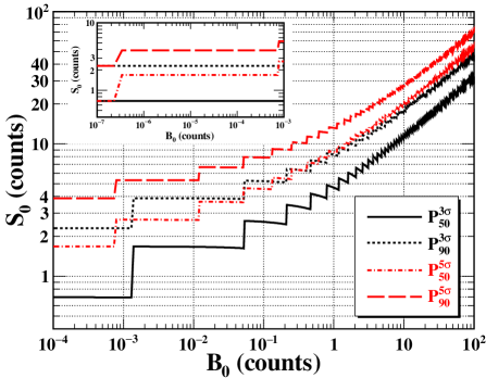
Figure 1: The variations of ${\rm S_{0}}$ versus ${\rm B_{0}}$ in discovery potential in counting experiments under the criteria ${\rm P}_{g}^{k\sigma}$, for $k{=}3,5$ and $g{=}50,90\%$. The inset displays contours at ${\rm B_{0}}{<}10^{\mbox{-}3}$. The first steps at lowest ${\rm B_{0}}$ correspond to the transition where an increase of $n_{obs}$ from 1 to 2 events is required to positively establish the signals.

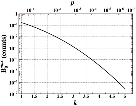
Figure 2: Variations of ${\rm B}_{0}^{max}$ which satisfies the zero-background condition as a function of $k$ and $p$. The contour is independent of $g$.

Poisson statistics is necessary in the complete formulation of the problem. For a given positive ${\rm B_{0}}$ as input and using ${\rm P_{50}^{3\sigma}}$ as illustration, the Poisson distribution ${\rm Poi}(i;\mu)$ is constructed with mean $\mu{=}{\rm B_{0}}$. Let $N_{obs}^{3\sigma}$ be the minimal integer number of observed events which provides ${\geq}3\sigma$ significance over a predicted average background ${\rm B_{0}}$. $N_{obs}^{3\sigma}$ satisfies the following equation:

$$\sum_{i=0}^{N_{obs}^{3\sigma}-1}{\rm Poi}(i;{\rm B_{0}})\geq(1-p)~{}.$$ (3)

from which the value of $N_{obs}^{3\sigma}$ can be determined. The output ${\rm S_{0}}$ is the minimal signal strength where a Poisson distribution with $\mu{=}({\rm B_{0}}{+}{\rm S_{0}})$ would give $N_{obs}^{3\sigma}$ or more events with $g{=}50\%$ probability:

$$\sum_{i=N_{obs}^{3\sigma}}^{\infty}{\rm Poi}(i;{{\rm B_{0}}{+}{\rm S_{0}}})=0.5~{}~{}.$$ (4)

The required ${\rm S_{0}}$ for criteria ${\rm P}_{g}^{k\sigma}$ due to different $k$ and $g$ are shown in Figure 1. The characteristic step-wise features are consequences of the discrete nature in Poisson statistics $-$ only integer $n_{obs}$ are observed in one measurement. The steps for ${\rm P_{50}^{3\sigma}}$ and ${\rm P_{90}^{3\sigma}}$ occur at the same ${\rm B_{0}}$. This corresponds to the same required $N_{obs}^{3\sigma}$ to meet the ${\geq}3\sigma$ ($p{\leq}0.00135$) criteria. More ${\rm S_{0}}$ events are necessary to establish a positive signal in ${\rm P_{90}^{3\sigma}}$ than ${\rm P_{50}^{3\sigma}}$ when $g$ increases from 50% to 90% in Eq. 4.

Signal and background events are indistinguishable experimentally. The ${\rm P}_{g}^{k\sigma}$ criteria and discreteness of Poisson statistics apply to $({\rm B_{0}}{+}{\rm S_{0}})$. However, the useful information to experiments is on the variation of ${\rm S_{0}}$ with ${\rm B_{0}}$. This explains the origin of the negative slopes between the steps in Figure 1.

A particular case of interest is the “zero-background condition” in which $n_{obs}{=}1$ event would qualify to be taken as a positive signal. The maximum ${\rm B_{0}}$ (denoted as ${\rm B}_{0}^{max}$) where such conditions apply correspond to the “first steps” in Figure 1. The dependence of ${\rm B}_{0}^{max}$ on $k$ and $p$ is depicted in Figure 2. The values of ${\rm B}_{0}^{max}$ and ${\rm S_{0}}$ under zero-background condition at different ${\rm P}_{g}^{k\sigma}$ are summarized in Table 1, which illustrates the effects of $k$ and $g$.

The values of ${\rm B}_{0}^{max}$ $-$ and in general the required $n_{obs}$ to establish positive signals at ${+}k\sigma$ excesses over background $-$ are described by Eq. 3 and are therefore independent of the choice of $g$. On the other hand, the required signal strength ${\rm S_{0}}$ at ${\rm B}_{0}^{max}$ is given by Eq. 4 and therefore has $g$-dependence.

Table 1: Summary of the ${\rm S_{0}}$ and ${\rm B}_{0}^{max}$ values in counting-only analysis with complete Poisson statistics at the zero-background condition where $n_{obs}{=}1$ event can establish a positive signal under the criteria ${\rm P}_{g}^{k\sigma}$.

		Excess over background
		$(~{}k\sigma~{})$
		${+}3\sigma$	${+}5\sigma$
${\rm B}_{0}^{max}$		0.00135	$2.85{\times}10^{\mbox{-}7}$
		${\rm S_{0}}$ at ${\rm B_{0}}{<}{\rm B}_{0}^{max}$
	50%	0.69
Sample Fraction
$(~{}g~{})$	90%	2.3

II.2 Continuous Approximation to Poisson Distribution

(a)

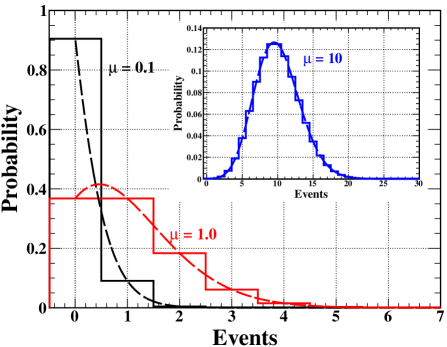
(b)

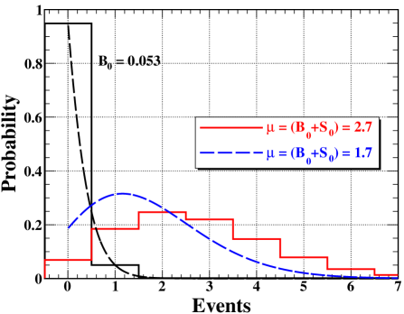
Figure 3: (a) Comparison of Poisson distribution in its complete formulation and continuous approximations in the cases of $\mu{=}{\rm B_{0}}{=}0.1,1,10$. (b) The $\mu{=}({\rm B_{0}}+{\rm S_{0}})$ distributions with ${\rm P_{50}^{3\sigma}}$ under both criteria at ${\rm B_{0}}{=}0.053$, showing their differences $-$ $\mu$=2.7(1.7) for complete Poisson (continuous approximation).

Continuous approximations to the Poisson distributions are derived by replacing Eq. 2 with the regularized incomplete gamma function:

$${\rm CPoi}({\leq}C;\mu)={\frac{\Gamma(C{+}1;\mu)}{\Gamma(C{+}1)}~{}~{},}$$ (5)

where $C$ is generalized to be a continuous variable. The summations of Eqs. 3&4 are replaced by Eq. 5, applicable for ${\rm B_{0}}{\geq}0$. This has been adopted to derive results to the sensitivity projection problem [3, 4, 5, 6, 7, 8, 9, 10].

The comparisons of the Poisson distribution ${\rm Poi}(n;\mu{=}{\rm B_{0}})$ and its continuous approximation is depicted in Figure 3a, showing cases of $\mu{=}0.1,1,10$ to illustrate behavior for different ranges. For large $\mu$, the continuous formulation approximates well to the discrete case, and approaches the Gaussian distribution.

Only integer results are possible in counting measurements, so that the criterion “${\geq}3\sigma$” is mostly satisfied as an inequality in the complete Poisson analysis. Illustrated in Figure 3b is an example of how ${\rm S_{0}}$ would differ with the two formulations, where the integration from zero of the histograms and dotted curves are different. The figure illustrates with the example of ${\rm B_{0}}$=0.053. Individual experiments would require $n_{obs}{\geq}3(2)$ to meet the “${\geq}3\sigma$” condition, while ${\rm P_{50}^{3\sigma}}$ would imply average ${\rm S_{0}}{=}2.64(1.64)$ under complete Poisson counting and continuous approximation, respectively.

Results on the dependence of ${\rm S_{0}}$ versus ${\rm B_{0}}$ from both formulations are depicted in Figure 4a. The ${\rm S_{0}}$ derived with complete Poisson statistics (${\rm S}_{0}^{Poi}$) is always larger than that from continuous approximation (${\rm S}_{0}^{cont}$), except at where equality (${=}3\sigma$) is met. The fractional decrease is depicted in Figure 4b by the black line, where $R_{0}^{Poi}{=}({{\rm S}_{0}^{cont}}{-}{{\rm S}_{0}^{Poi}})/{{\rm S}_{0}^{Poi}}$. It can be seen that the continuous approximation always underestimate the necessary strength to establish a signal. The deviation can be as much as 60% at low background (${\rm B_{0}}{\sim}10^{\mbox{-}3}$), but reduced to within 3% at large statistics of ${\rm B_{0}}{\gtrsim}100$.

(a)

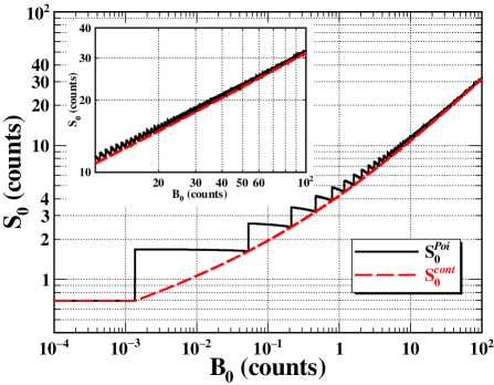
(b)

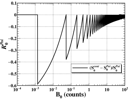
Figure 4: (a) Comparison between counting-only with complete Poisson (${\rm S}_{0}^{Poi}$) and continuous approximation (${\rm S}_{0}^{cont}$) in defining the ${\rm P_{50}^{3\sigma}}$ sensitivity. (b) Relative change ($R_{0}^{Poi}$) of ${\rm S}_{0}^{cont}$ relative to ${\rm S}_{0}^{Poi}$.

III Likelihood Analysis

In Section II, event count is used as “test statistic” [13, 15]. This is a straight forward choice for experiments that measure a single integer value as the only output. However, in experiments with measurements of multiple variables, the Poisson counting method is insufficient to extract complete information available in the signal and background. An alternative and more comprehensive formulation of test statistic is therefore necessary.

A test statistic is a mapping from an experimental outcome with multiple values to a single real number. The optimal test statistic is the likelihood ratio, following the Neyman–Pearson lemma [16].

In this analysis, we adopt log likelihood ratio (LLR) in Sections III.1&III.2 to be the test statistic where $S{=}{\rm S_{0}}$ is a free parameter and $B{=}{\rm B_{0}}$ is fixed. For cases where the uncertainties in $B$ are considered as in Sections III.5&IV, a variant of LLR with additional “nuisance parameter” (called log profile likelihood ratio) is used.

III.1 Formulation and Single Integer Counting

The counting-only likelihood function is given by:

$$\mathscr{L}_{C} ~{}\equiv~{} \mathscr{L}(S|N,B)$$

$$~{}=~{} \frac{e^{-(B+S)}(B+S)^{N}}{N!}.$$

Following conventional notations of Refs. [11, 15], the LLR, denoted by $q_{0}$, is defined as

$$q_{0}~{}~{}{\equiv}~{}~{}{t(S{=}0)}~{}=~{}-2~{}{\rm ln}\left[\frac{\mathscr{L}(S{=}0)}{\mathscr{L}(\hat{S})}\right]~{},$$ (7)

in which $\hat{S}$ is the value of $S{\in}(0,\infty)$ that $\mathscr{L}(S)$ is maximized for given $N$ and at a fixed $B{=}{\rm B_{0}}$ value. The $q_{0}$ is defined as a test statistic ($t$) which serves as the foundation of a statistical test under the special case where $S{=}0$.

We are interested in this work to quantitatively assess the significance of a measurement in supporting a discovery scenario. Accordingly, the data set has to be tested against the null hypothesis ($H_{0}$) case of $S{=}0$. Consistent data set of $H_{0}$ with $S{=}0$ will give $q_{0}{\rightarrow}0$ whereas large $q_{0}$-values imply deviation from $H_{0}$. The alternative hypothesis ($H_{1}$) characterizes the case with $S{=}{\rm S_{0}}{>}0$, where ${\rm S_{0}}$ is the mean signal strength. If a significant fraction of a data set generated by $H_{1}$ gives large $q_{0}$-values, $H_{0}$ would have to be rejected.

The probability distributions of $q_{0}$ for given ${\rm B_{0}}$ are evaluated from data sets simulated with $\mathscr{L}_{C}$ having $N{=}{\rm B_{0}}{+}{\rm S_{0}}$ events: (i) $P(q_{0}|H_{0})$ corresponding to $H_{0}$ with data at ${\rm S_{0}}{=}0$, and (ii) $P(q_{0}|H_{1})$ corresponding to $H_{1}$ with data at non-zero $S{=}{\rm S_{0}}{>}0$.

Standard statistics variables are adopted to quantify statistical consistency with hypotheses in $P(q_{0}|H_{0})$ and $P(q_{0}|H_{1})$. Data with $q_{0}{<}t_{\alpha}$ are considered to be within the “acceptance interval” consistent with $H_{0}$, where $t_{\alpha}$ is a boundary to the “size of test”[13] (also called the Type-1 error and denoted as $\alpha$), a pre-defined value corresponding to the probability that the data set which is inconsistent with $H_{0}$, or equivalently when $q_{0}$ is rejected to be $H_{0}$:

$$\alpha\equiv\int_{t_{\alpha}}^{\infty}~{}P(q_{0}|H_{0})~{}dq_{0}~{}.$$ (8)

The “power of test” [13] corresponds to ($1{-}\beta$), where $\beta$ (also called the Type-2 error) is the probability of $q_{0}$ within the acceptance region of $H_{0}$ in the scenario where the hypothesis $H_{1}$ is true. It can be expressed as:

$$\beta\equiv\int_{0}^{t_{\alpha}}~{}P(q_{0}|H_{1})~{}dq_{0}~{}~{}.$$ (9)

In counting experiments, integrations in Eqs. 8&9 should be replaced by summations, such that:

$$\alpha ~{}\geq~{} \sum_{q_{0}\geq t_{\alpha}}P(q_{0}|H_{0})~{},~{}{\rm and}$$

$$\beta ~{}=~{} \sum_{q_{0}\leq t_{\alpha}}P(q_{0}|H_{1})~{}.$$ (10)

As a result of discreteness relevant and crucial to low-statistics counting, $\alpha$ in general cannot be exactly equal to, and should instead over-cover, the “size of test”. Therefore, $\alpha$ should be defined instead as an inequality. On the contrary, the $\beta$-condition depends on the mean signal strength ${\rm S_{0}}$ which is a real number, so that it can be satisfied as an equality.

The criteria ${\rm P}_{g}^{k\sigma}$ defined in this work corresponds to the matching of $p{=}\alpha$ and $g{=}(1{-}\beta)$ to the standard statistical variables. Accordingly, ${\rm P_{50}^{3\sigma}}$ implies the choice of $t_{\alpha}$ which leads to $p{=}0.00135$ for $P(q_{0}|H_{0})$ with $q_{0}{\in}[0,t_{\alpha}]$. Experiments with $q_{0}{\in}[t_{\alpha},\infty]$ are inconsistent with $H_{0}$. In addition, there is $(1{-}\beta){=}50\%$ probability to have $q_{0}{\in}[t_{\alpha},\infty]$ in $P(q_{0}|H_{1})$ so that the experiment is recognized to have observed positive signals.

As a result of the discreteness of single-value integer counting, the count to $q_{0}$ mapping is always one to one at $\hat{S}{>}0$. Examples of $P(q_{0}|H_{0})$ and $P(q_{0}|H_{1})$ distributions for LLR counting analysis with $\mathscr{L}_{C}$ are shown in Figures 5a&b, which describe cases of low- and high-statistics, respectively.

In the absence of additional measurables, the LLR analysis on $\mathscr{L}_{C}$ results in ${\rm S_{0}}[{\mathscr{L}_{C}}]$ (signal strength of counting-only LLR analysis) which are identical to ${\rm S}_{0}^{Poi}$ derived by the complete Poisson counting analysis. The counting-only results of Figure 1 and Figures 4a&b can be derived by both formulations in Section II.1 and Section III.1.

(a)

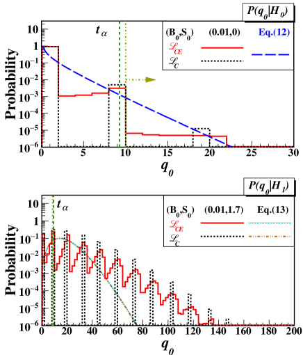
(b)

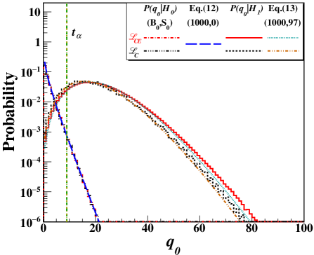
Figure 5: Distributions of test statistic $q_{0}$ for simulated data with null [$P(q_{0}|H_{0})$] and alternative [$P(q_{0}|H_{1})$] hypotheses for negligible ${\rm B_{0}}$ uncertainties: (a) depicts a low-${\rm B_{0}}$ case with $({\rm B_{0}},{\rm S_{0}}){=}(0.01,0)$ and $(0.01,1.7)$ while (b) is a large-${\rm B_{0}}$ case with $({\rm B_{0}},{\rm S_{0}}){=}(1000,0)$ and $(1000,97)$. The acceptance criteria specified by $t_{\alpha}$ are displayed. The approximations of Eqs. 12&III.3 are superimposed, verifying that they match $P(q_{0}|H_{0})$ and $P(q_{0}|H_{1})$ for large but fail for small $({\rm B_{0}},{\rm S_{0}})$.

III.2 Extended Likelihood with Additional Measurables

In realistic applications, such as $0\nu\beta\beta$ experiments to be discussed in Section IV, the observables typically include energy. Without loss of generality, we take energy of an event to be the additional available observable. The studied scenario is with signal events having known mono-energetic ${\rm E_{0}}$ smeared by experimental resolution characterized by Gaussian peaks with known width $-$ RMS and FWHM (full-width-half-maximum) denoted by $\sigma_{\rm E_{0}}$ and $\Delta_{\rm E_{0}}{(\equiv 2.355{\times}\sigma_{\rm E_{0}})}$, respectively. The background is known and is a constant independent with energy, characterized by ${\rm B_{0}}$ and $\sigma_{B}$ denoting, respectively, the expected background count and its RMS uncertainty. An RoI has to be specified in the analysis in such experiments, in which additional energy measurements are available. A natural choice would be $({\rm E_{0}}{\pm}\rm N_{\sigma}\sigma_{\rm E_{0}})$ where the variable $\rm N_{\sigma}$ would parametrize the interval width of the RoI. Background is then quantified as $({\rm B_{0}}/\sigma_{\rm E_{0}})$ in units of counts-per-RMS, as compared to the exclusive counting-only cases of ${\rm B_{0}}$(counts) in Section II.

In the limit of $\sigma_{B}{\ll}B$ where the background is accurately predicted, the likelihood function of a signal $S$ given a known background profile $B$ and a data set $\mathbb{E}$ with $N$ events with measured energy $E_{i}(i=1,N)$ can be described by the extended likelihood function:

$$\mathscr{L}_{CE} ~{}\equiv~{} \mathscr{L}(S|\mathbb{E},B)$$

$$~{}=~{} \frac{e^{-(B+S)}(B+S)^{N}}{N!}\times$$

$$\prod_{i=1}^{N}\left[\frac{B\cdot{f_{B}(E_{i})}+S\cdot f_{S}(E_{i})}{(B+S)}\right]~{},$$

where $f_{B}$ and $f_{S}$ are normalized probability density functions of, respectively, background and signal, such that $\int_{\rm RoI}{f_{B}(E)dE}{=}1$ and $\int_{\rm RoI}{f_{S}(E)dE}{=}1$.

In our adopted $0\nu\beta\beta$-inspired scenario, $B{=}{\rm B_{0}}$ and $f_{B}$ is a constant independent of energy, while $f_{S}$ is a Gaussian with known mean and width. Results on $\mathscr{L}_{CE}(S)$ from Eq. III.2 is independent on the choice of RoI, so long as it covers the entire signal region$-$ ${\rm RoI}(\mathscr{L}_{CE}){=}{\rm E_{0}}{\pm}4\sigma_{\rm E_{0}}$ is selected in this analysis, with which $\varepsilon_{\rm RoI}(\mathscr{L}_{CE}){=}0.9999$.

The LLR of Eq. 7 is selected [1] as the test statistic ($q_{0}$) [11, 12, 13, 15]. Unlike those from counting analysis of Eq. 7, probability distributions of $q_{0}$ do not have analytical form for both the $H_{0}$ and $H_{1}$ hypotheses, and have to be generated by simulation. Approximation methods can be used in the special cases of large samples, as discussed in Section III.3.

The case of $\sigma_{B}{\ll}B$ was first studied. A total of 50-million experiments are generated for each $\mathbb{E}$ with different input values of ${\rm S_{0}}$. The number of background ($N_{B}$) and signal ($N_{S}$) events for individual experiment follow Poisson statistics: ${\rm Poi}(N_{B}|{\rm B_{0}})$ and ${\rm Poi}(N_{S}|{\rm S_{0}})$, respectively, while their energy distributions follow $f_{B}(E)$ and $f_{S}(E)$ within the RoI. The total number of events, $N{=}N_{B}{+}N_{S}$, varies with each experiment. The $\hat{S}$-values which maximize $\mathscr{L}$ for individual experiments are derived, from which the $q_{0}$-values of Eq. 7 are evaluated. Their distributions over large number of experiments in $P(q_{0}|H_{0})$ and $P(q_{0}|H_{1})$ corresponds to the probability densities where $q_{0}$ is consistent with $H_{0}$ and $H_{1}$, respectively.

Displayed in Figure 5a are distributions of $P(q_{0}|H_{0})$ and $P(q_{0}|H_{1})$ as functions of $q_{0}$ in both $\mathscr{L}_{C}$ and $\mathscr{L}_{CE}$ for a low-statistics case, where $({\rm B_{0}},{\rm S_{0}}){=}(0.01,0)$ and $(0.01,1.7)$. The analogous high-statistics case at $({\rm B_{0}},{\rm S_{0}}){=}(1000,0)$ and $(1000,97)$ is shown in Figure 5b. As additional energy information is incorporated to the analysis, $P(q_{0}|H_{0})$ and $P(q_{0}|H_{1})$ are smeared out in low statistics, while changes are minor in high statistics.

The $t_{\alpha}$-values corresponding to ${\geq}3\sigma$ upward excesses from $H_{0}$ are marked in Figures 5a&b. In particular in the high statistics limit where ${\rm B_{0}}{=}1000$ in Figure 5b, $P(q_{0}|H_{0})$ approximates to $\chi^{2}$-distribution and $t_{\alpha}{\rightarrow}9$.

III.3 Approximate Distribution of $q_{0}$ for Large-Samples

Following the formulation by Wilks [17] and Wald [18], $P(q_{0}|H_{0})$ or $P(q_{0}|H_{1})$ can be simplified in the large-sample limit, where Poisson distributions can be approximated by Gaussian. Computing resources in simulations can therefore be saved by the use of analytic equations when results are evaluated from input spanning large parameter space.

When $S\geq 0$, $P(q_{0}|H_{0})$ is given by half $\chi^{2}$-distribution for one degree of freedom plus a half $\delta$-function:

$$P(q_{0}|H_{0})\approx\frac{1}{2}\delta(q_{0})+\frac{1}{2}\frac{1}{\sqrt{2\pi}}\frac{1}{\sqrt{q_{0}}}e^{-q_{0}/2}~{},$$ (12)

while $P(q_{0}|H_{1})$ is described by non-central $\chi^{2}$-distribution for one degree of freedom:

$$P(q_{0}|H_{1}) \approx (1-\Phi(\sqrt{\Lambda}))\delta(q_{0})$$

$$+\frac{1}{2}\frac{1}{\sqrt{2\pi}}\frac{1}{\sqrt{q_{0}}}e^{-(\sqrt{q_{0}}-\sqrt{\Lambda})^{2}/2}~{},$$

where $\Lambda$ is the non-centrality parameter, and $\Phi$ is cumulative Gaussian distribution. The $\Lambda$ is the $q_{0}$ value of most probable $-$ that is, Asimov $-$ data set [11].

Binned likelihood function is used in the evaluation of $\Lambda$:

$$\mathscr{L}(S|\{n_{i}\},B)\approx\prod_{i=1}^{n}{\rm Poi}(n_{i}|F(E_{i}|S,B))~{},$$ (14)

where

$$F(E_{i}|S,B)=\left[~{}B\cdot{f_{B}(E_{i})}+S\cdot f_{S}(E_{i})~{}\right]\cdot w(E_{i})$$ (15)

is the expected counts in the $i^{th}$-bin with bin size $w(E_{i})$, $n_{i}$ is the measured count and $E_{i}$ is the mean energy. We note that likelihood expression of Eq. 14 differs from Eq. III.2 by a scaling constant which is canceled out when taking likelihood ratio.

The Asimov data set is therefore the expected count in each bin:

$$n_{i}=F(E_{i}|{\rm S_{0}},{\rm B_{0}})~{},$$ (16)

where ${\rm S_{0}}$, ${\rm B_{0}}$ are the input values to generate the simulated data. Accordingly, the $\Lambda$-value is the likelihood ratio:

$$\Lambda\approx-2~{}{\rm ln}\left[\frac{\mathscr{L}(S{=}0|B,n_{i}{=}F(E_{i}|{\rm S_{0}},{\rm B_{0}}))}{\mathscr{L}(\hat{S}|B,n_{i}{=}F(E_{i}|{\rm S_{0}},{\rm B_{0}}))}\right]~{},$$ (17)

with the $n_{i}!$ factorial terms in denominator and numerator canceled out.

The approximations of $P(q_{0}|H_{0})$ and $P(q_{0}|H_{1})$ by Eqs. 12&III.3 in the low- and high-statistics regimes are superimposed in Figures 5a&b, respectively. It can be seen that for the high-statistics limit, the approximations match well with the simulation results of $P(q_{0}|H_{0})$ and $P(q_{0}|H_{1})$, but they deviate significantly in the low-statistics regimes.

(a)

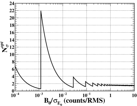
(b)

Figure 6: (a) Variation of ${\rm N}^{opt}_{\sigma}$ versus $({\rm B_{0}}/\sigma_{\rm E_{0}})$ in counting-only analysis for which the required ${\rm S_{0}}$ to satisfy ${\rm P_{50}^{3\sigma}}$ are at minimum. The RoIs are defined by intervals ${\rm E_{0}}{\pm}\rm N_{\sigma}\sigma_{\rm E_{0}}$. (b) Comparison of ${\rm S_{0}}$ versus $({\rm B_{0}}/\sigma_{\rm E_{0}})$ at ${\rm N}^{opt}_{\sigma}$ with those at fixed $\rm N_{\sigma}{=}1,2,3$.

(a)

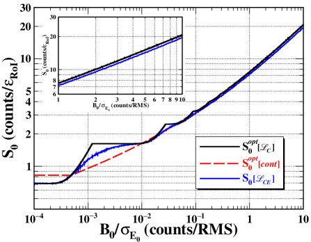
(b)

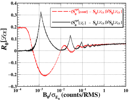
Figure 7: Sensitivities of $({\rm S_{0}}/\varepsilon_{\rm RoI})$ as a function of $({\rm B_{0}}/\sigma_{\rm E_{0}})$: (a) On $\mathscr{L}_{CE}$ by LLR analysis with complete information incorporated, choosing ${\rm RoI}(\mathscr{L}_{CE}){=}{\rm E_{0}}{\pm}4\sigma_{\rm E_{0}}$. These are compared with those counting-only analysis via $\mathscr{L}_{C}$ and continuously approximation for the optimal RoI of ${\rm E_{0}}{\pm}{\rm N}^{opt}_{\sigma}\sigma_{\rm E_{0}}$. (b) The deviations of ${\rm S}_{0}^{opt}[{\mathscr{L}_{C}}]$ and ${\rm S}_{0}^{opt}[cont]$ relative to ${\rm S_{0}}[{\mathscr{L}_{CE}}]$, denoted as $R_{0}[{\mathscr{L}_{CE}}]$.

III.4 Comparison between Counting and Extended Likelihood Analysis

Taking experiments where where both counts and energy are measured, the required ${\rm S_{0}}$-strength to achieve the ${\rm P_{50}^{3\sigma}}$ discovery potential criteria are derived. Several analysis schemes are compared: (i) with the LLR analysis using $\mathscr{L}_{CE}$ of Section III.2 exploiting both information, denoted ${\rm S_{0}}[\mathscr{L}_{CE}]$, (ii) with a counting-only analysis via $\mathscr{L}_{C}$ of Section III.1 discarding the available energy information, denoted ${\rm S_{0}}[\mathscr{L}_{C}]$ (this is equivalent to ${\rm S}_{0}^{Poi}$ of Section II.1 when the RoI intervals and $\varepsilon_{\rm RoI}$ are taken into account [14]), and (iii) with a counting-only analysis the continuous approximation of Section II.2 [3, 4, 5, 6, 7, 8, 9, 10], denoted ${\rm S_{0}}[cont]$.

As noted in Section III.2, the sensitivities on ${\rm S_{0}}[\mathscr{L}_{CE}]$ is independent on the choice of RoI, so long as $\varepsilon_{\rm RoI}{\simeq}1$, such as ${\rm RoI}(\mathscr{L}_{CE}){=}{\rm E_{0}}{\pm}4\sigma_{\rm E_{0}}$. On the contrary, the counting-only analysis of (ii) and (iii) depend on the choice of RoI as parametrized by $\rm N_{\sigma}$. The optimal $\rm N_{\sigma}$ (denoted ${\rm N}^{opt}_{\sigma}$) which gives minimal ${\rm S_{0}}[\mathscr{L}_{C}]({\equiv}{\rm S}_{0}^{opt}[\mathscr{L}_{C}]$) and ${\rm S_{0}}[cont]({\equiv}{\rm S}_{0}^{opt}[cont]$) can be evaluated.

The variation of ${\rm N}^{opt}_{\sigma}$ as a function of $({\rm B_{0}}/\sigma_{\rm E_{0}})$ is displayed in Figure 6a. As noted in Ref. [4] and verified in our results, the choice of ${\rm N}^{opt}_{\sigma}{=}1.4$ is optimal at large $({\rm B_{0}}/\sigma_{\rm E_{0}}){\gtrsim}1$. The ranges of optimal RoIs for low $({\rm B_{0}}/\sigma_{\rm E_{0}})$ vary broadly due to large fluctuations in low counts and the discreteness of Poisson statistics. Depicted in Figure 6b is ${\rm S}_{0}^{opt}[{\mathscr{L}_{C}}]$ superimposed with the cases of fixed RoI for intervals ${\rm E_{0}}{\pm}\rm N_{\sigma}\sigma_{\rm E_{0}}$ (where $\rm N_{\sigma}{=}1,2,3$) corresponding to $\varepsilon_{\rm RoI}{=}68.3\%,95.5\%,99.7\%$, respectively.

The results of the three analysis schemes are compared in Figure 7a. The deviations of ${\rm S}_{0}^{opt}[cont]$ and ${\rm S}_{0}^{opt}[\mathscr{L}_{C}]$ relative to ${\rm S_{0}}[\mathscr{L}_{CE}]$ are depicted in Figure 7b.

While the features can be expected, the results verify and quantify that in experiments incorporating additional energy information, the discovery potentials are enhanced due to ${\rm S}_{0}[{\mathscr{L}_{CE}}]{\leq}{\rm S}_{0}^{opt}[{\mathscr{L}_{C}}]$ which implies less events are required to establish positive signals.

At the low-statistics regime $[({\rm B_{0}}/\sigma_{\rm E_{0}}){\lesssim}0.01]$, this originates from that the ${\rm P_{50}^{3\sigma}}$ criteria can be satisfied for all ${\rm B_{0}}$ in $\mathscr{L}_{CE}$, which is not the case for counting-only analysis in $\mathscr{L}_{C}$ due to “over-coverage” (the $p{=}0.00135$ criteria cannot be met). At high statistics $[({\rm B_{0}}/\sigma_{\rm E_{0}}){\gtrsim}0.1]$, requirements for the energy values to match a pre-defined Gaussian peak provide the dominant constraints.

At low $({\rm B_{0}}/\sigma_{\rm E_{0}}){\sim}10^{\mbox{-}3}$, the ${\rm S}_{0}^{opt}[cont]$ can underestimate the required strength of ${\rm S_{0}}[\mathscr{L}_{CE}]$ by as much as 20%. The ${\rm S}_{0}^{opt}[\mathscr{L}_{C}]$, on the other hand, can be overestimated by as much as 30% and is larger than ${\rm S_{0}}[\mathscr{L}_{CE}]$ for all $({\rm B_{0}}/\sigma_{\rm E_{0}}){>}5{\times}10^{\mbox{-}4}$. At large $({\rm B_{0}}/\sigma_{\rm E_{0}}){>}1$, both derivations with counting-only analysis give consistent results which overestimate ${\rm S_{0}}[\mathscr{L}_{CE}]$ by $\sim$6%.

III.5 Effects of Background Uncertainties

(a)

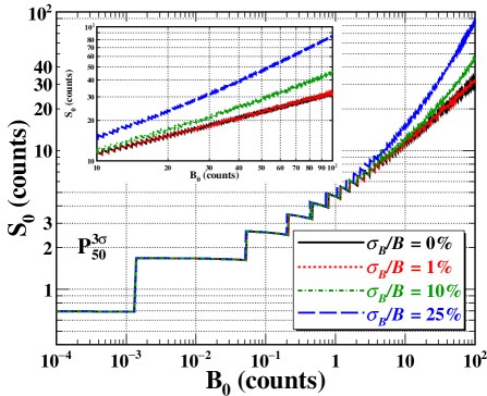
(b)

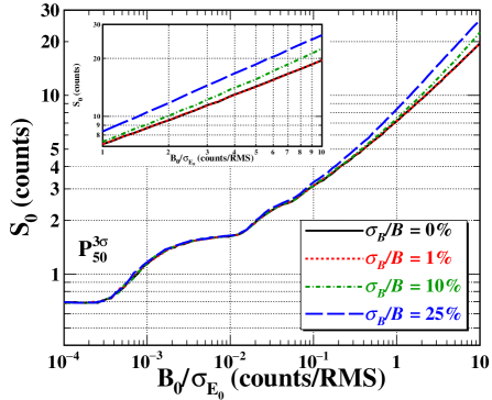
(c)

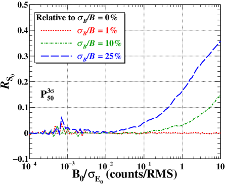
Figure 8: The effects on the sensitivities on ${\rm S_{0}}$ defined by ${\rm P_{50}^{3\sigma}}$ due to background uncertainties ($\sigma_{B}/B$) (a) in counting-only analysis with $\mathscr{L}_{C}$, and (b) in LLR analysis with energy information $(\mathscr{L}_{CE})$ when the signal is an energy peak with Gaussian distribution, and the selected ${\rm RoI}(\mathscr{L}_{CE}){=}{\rm E_{0}}{\pm}4\sigma_{\rm E_{0}}$. (c) The fractional increase of ${\rm S_{0}}$ in $\mathscr{L}_{CE}$ (denoted as $R_{{\rm S_{0}}}$) due to non-zero $(\sigma_{B}/B)$ relative to the case of zero uncertainty.

In realistic experiments, the background $B$ is usually not precisely known and can be characterized with an uncertainty $\sigma_{B}$. That background knowledge can be described as auxiliary measurement channels (for instance, from simulations, prototype measurements, extrapolations from non-RoI regions) in the likelihood analysis.

The likelihood with an additional auxiliary channel can be described by another Poisson distribution ${\rm Poi}(n_{0}|{\tau}B)$, and expressed as [11, 12, 13]

$$\mathscr{L}_{CEB} ~{}\equiv~{} \mathscr{L}(S,B|\mathbb{E})$$

$$= \frac{e^{-(B+S)}(B+S)^{N}}{N!}\frac{e^{-{\tau}B}({\tau}B)^{n_{0}}}{n_{0}!}$$

$$\times\prod_{i=1}^{N}\left[\frac{B\cdot{f_{B}(E_{i})}+S\cdot f_{S}(E_{i})}{(B+S)}\right]~{},$$

where $\tau$ is the ratio of data size of auxiliary measurement channel relative to the main measurement channel, such that the RMS uncertainty in $B$ is $\sigma_{B}{=}\sqrt{{\tau}B}/\tau$.

For non-zero $\sigma_{B}$, additional values of $n_{0}$ for this auxiliary measurement are generated alongside ${\rm Poi}(N_{B}|{\rm B_{0}})$, ${\rm Poi}(N_{S}|{\rm S_{0}})$ as well as data sets $\mathbb{E}(H_{0})$ and $\mathbb{E}(H_{1})$ for Eq. III.5. The LLR for test statistic of Eq. 7 is extended to:

$$q_{0}\equiv t(S=0){=}{\rm-2~{}ln}\left[\frac{\mathscr{L}_{CEB}(S=0,\hat{\hat{B}})}{\mathscr{L}_{CEB}(\hat{S},\hat{B})}\right],$$ (19)

in which $\hat{\hat{B}}$ is, for given $\mathbb{E}$, the value of $B$ that maximizes $\mathscr{L}_{CEB}(S,B)$ in $B{\in}(0,\infty)$ at $S{=}0$ and $(\hat{S},\hat{B})$ is the $(S,B)$ that maximizes $\mathscr{L}_{CEB}(S,B)$ in $S{\in}(0,\infty)$ and $B{\in}(0,\infty)$.

The Asimov data set includes $n_{0}{=}{\tau}{\rm B_{0}}$ in addition to the conditions of Eq. 16. The binned likelihood function can be expressed as:

$$\begin{split}\mathscr{L}(S|\{n_{i}\},B)\approx\hskip 142.26378pt\\ \left[~{}\prod_{i=1}^{n}{\rm Poi}(n_{i}|F(E_{i}|S,B))~{}\right]\cdot{\rm Poi}(n_{0}|{\tau}B)~{}~{}.\end{split}$$ (20)

An LLR analysis is performed on likelihood functions of $\mathscr{L}_{C}$ in Eq. III.1 and $\mathscr{L}_{CE}$ in Eq. III.2 with uncertainty term incorporated in $\mathscr{L}_{CEB}$ in Eq. III.5. Effects of a non-zero $(\sigma_{B}/B)$ are studied through the $q_{0}$ distributions for $P(q_{0}|H_{0})$ and $P(q_{0}|H_{1})$ in both low and high statistics, analogous to Figures 5a&b. The expected signal counts that meet the ${\rm P_{50}^{3\sigma}}$ criteria for different $(\sigma_{B}/B)$ values to the count-only and count-plus-energy cases, respectively, are depicted in Figures 8a&b. The fractional increase of ${\rm S_{0}}$ in $\mathscr{L}_{CE}$ due to non-zero $(\sigma_{B}/B)$ relative to the case of zero uncertainty is given in Figure 8c.

It can be seen that at the low-statistics regime (${\rm B_{0}}{<}1$ within RoI=${\rm E_{0}}{\pm}4\sigma_{\rm E_{0}}$) the effects of $\sigma_{B}$ are negligible. The reason is that statistical fluctuations of small numbers in a single measurement dominate over the inadequate knowledge of the background. There are notable increases to the required ${\rm S_{0}}$ in high statistics due to $\sigma_{B}$ uncertainties, and the impact is larger in $\mathscr{L}_{C}$ than in $\mathscr{L}_{CE}$. A $(\sigma_{B}/B){{=}}10\%$ uncertainty will give rise to increase in ${\rm S_{0}}$ by 45% and 17% at ${\rm B_{0}}{{=}}100$ within RoI for counting-only and counting-plus-energy analysis, respectively. The availability of the additional energy measurements makes the evaluation of ${\rm S_{0}}$ more robust and less vulnerable to background uncertainties.

We note that $\sigma_{B}$ depends on the knowledge on $B$ from the auxiliary data prior to the experiments. In practice, with improving data quality and increasing data size during the experiments, $\sigma_{B}$ can be expected to be further reduced.

IV Case Study: Neutrinoless Double Beta Decay

(a)                                                                       (b)

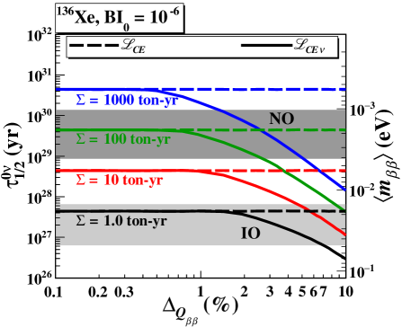
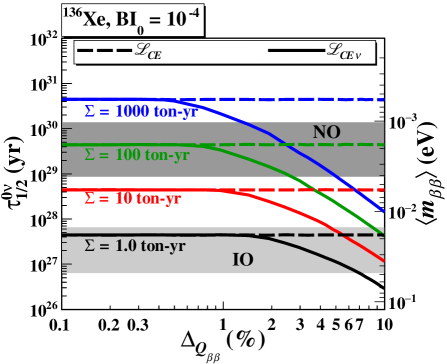
(c)                                                                       (d)

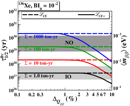
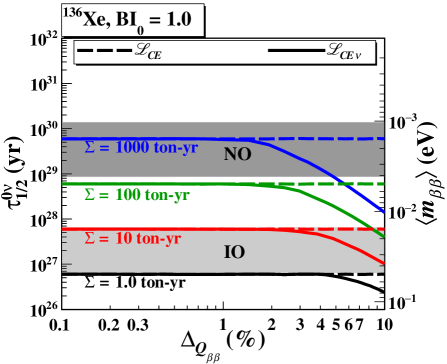
Figure 9: Combined background LLR analysis for $\rm{}^{136}Xe$ in $(\Delta_{Q_{\beta\beta}},\uptau^{0\nu}_{\scaleto{1/2}{5pt}})$ space at different contours $\Sigma{=}1,10,100,1000{~{}}{\rm ton\mbox{-}yr}$ taking ${\rm BI_{0}}$= (a) $10^{-6}$, (b) $10^{-4}$, (c) $10^{-2}$, and (d) 1 ${\rm counts}/(\rm FHWM\mbox{-}{\rm ton\mbox{-}yr})$ under the specific case where uncertainties in the expected ambient background are negligible, or $(\sigma_{B}/B){=}0\%$. Case (a) is, in particular, effectively the zero ambient background condition. Predicted $\langle m_{\beta\beta}\rangle$ ranges for neutrino mass IO and NO [19, 20], following the matrix elements models prescribed in Ref. [14] are superimposed. Scenarios with $2\nu\beta\beta$ background switched off are displayed as dotted lines to illustrate individual contributions from both background components. The $2\nu\beta\beta$ process is the leading background for increasing $\Delta_{Q_{\beta\beta}}$ beyond the divergent points.

A case study was performed to make sensitivity projections on future $0\nu\beta\beta$ experiments with profile likelihood, similar to previous work in Ref. [21]. This study serves to illustrate how the formulation and algorithms developed in this work can be applied in practice. A particular isotope and theoretical model are selected as example. Detailed comparisons taken into account the variety of target isotopes, experimental design specifications, theoretical modeling and practical resource-effectiveness are issues beyond the theme and scope of this work.

The process $0\nu\beta\beta$ [22, 9] is a lepton-number violating process involving the decays of isotope $A_{\beta\beta}(N,Z)$ to two electrons:

$${}^{N}_{Z}A_{\beta\beta}~{}\rightarrow~{}_{Z+2}^{N-2}A~{}+~{}2e^{-}~{}~{}.$$ (21)

Experimental signature is a monoenergetic energy peak at the decay Q-value ($Q_{\beta\beta}$). The FWHM of the $0\nu\beta\beta$-peak is denoted by $\Delta_{Q_{\beta\beta}}$ in %.

The decay half-life $\uptau^{0\nu}_{\scaleto{1/2}{5pt}}$ can be derived from measurements via:

$${\uptau^{0\nu}_{\scaleto{1/2}{5pt}}}~{}=~{}{{\rm ln~{}2}}\cdot\left[\frac{N_{A}}{(N+Z)}\right]\cdot\left[\frac{\Sigma}{S_{obs}/\varepsilon_{\rm RoI}}\right]~{},$$ (22)

where $N_{A}$ is the Avogadro Number, $\Sigma$ denotes the combined exposure typically expressed in units of ton-year (${\rm ton\mbox{-}yr}$), and $S_{obs}$ is the observed strength of the $0\nu\beta\beta$ peak. For simplicity, we take the ideal case where both isotopic abundance and experimental signal efficiency are 100%. The realistic exposure relative to the ideal one can be evaluated by corrections on these two parameters [14].

The measurable is related to neutrino masses via:

$$\left[\frac{1}{\uptau^{0\nu}_{\scaleto{1/2}{5pt}}}\right]~{}=~{}G^{0\nu}~{}g_{A}^{4}~{}|M^{0\nu}|^{2}~{}\left|\frac{\langle m_{\beta\beta}\rangle}{m_{e}}\right|^{2}~{},$$ (23)

where $m_{e}$ is the electron mass, $g_{A}$ is the effective axial vector coupling [23, 24], $G^{0\nu}$ is a known phase space factor [25] due to kinematics, $|M^{0\nu}|$ is the nuclear physics matrix element [26], while $\langle m_{\beta\beta}\rangle$ is the effective Majorana neutrino mass. To connect $|M^{0\nu}|$ with $\langle m_{\beta\beta}\rangle$, we adopt the model of Ref. [27] which observed that $\left[|M^{0\nu}|^{2}\cdot G^{0\nu}\right]$ can be approximated by a constant at fixed $\langle m_{\beta\beta}\rangle$ independent of the $0\nu\beta\beta$ candidate isotopes. Measurements in $\uptau^{0\nu}_{\scaleto{1/2}{5pt}}$ can then be translated to sensitivities in $\langle m_{\beta\beta}\rangle$ and be compared to the predicted ranges of neutrino mass Inverted and Normal Ordering (IO and NO) [19, 20].

Two background channels are considered: (i) ambient background which is assumed to be constant at $Q_{\beta\beta}$, and (ii) background due to two-neutrino double beta decay ($2\nu\beta\beta$) which leaks into the $0\nu\beta\beta$ peaks due to non-zero energy resolution of $\Delta_{Q_{\beta\beta}}$. Other background such as cosmogenic-induced events and solar neutrino interactions can be incorporated in future research, by expanding the constant ambient background conditions to include additional spectral components with energy dependence.

Following conventions [4, 28, 29], the ambient background is parametrized by the “Background Index” (${\rm BI_{0}}$) defined as:

$${\rm BI_{0}}~{}\equiv~{}\frac{{\rm B_{0}}(\Delta_{Q_{\beta\beta}})}{\Sigma}$$ (24)

which is the background in the FWHM energy range $\Delta_{Q_{\beta\beta}}$ around $Q_{\beta\beta}$ per ton-year of exposure, with dimension [${\rm counts}/(\rm FHWM\mbox{-}{\rm ton\mbox{-}yr})$]. Background levels expressed in ${\rm BI_{0}}$ are universally applicable to comparing sensitivities of different $0\nu\beta\beta$-experiments on a variety of the 0$\nu\beta\beta$ candidate isotope.

(a)                                                                       (b)

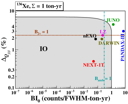
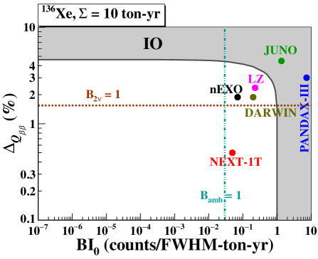
(c)                                                                       (d)

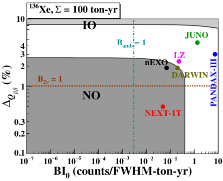
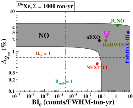
Figure 10: Requirements in $({\rm BI_{0}},\Delta_{Q_{\beta\beta}})$ space for $0\nu\beta\beta$ experiments with $\rm{}^{136}Xe$ to achieve ${\rm P_{50}^{3\sigma}}$, for $\Sigma$ at (a) 1, (b) 10, (c) 100 and (d) 1000 ton-yr, under the specific case where uncertainties in the expected ambient background are negligible, or $(\sigma_{B}/B){=}0\%$. Detector performance parameters in $({\rm BI_{0}},\Delta_{Q_{\beta\beta}})$ for the coming generation of $\rm{}^{136}Xe$-projects [21, 30, 31, 32, 33] are superimposed. The ${\rm B}_{2\nu}{=}1$ and ${\rm B}_{\rm amb}{=}1$ contours correspond to, respectively, where the first $2\nu\beta\beta$ and ambient background event would appear within ${\rm RoI}{=}Q_{\beta\beta}{\pm}4\sigma_{\rm E_{0}}$.

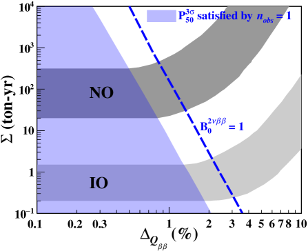
Figure 11: The conditions, represented by the white region, under which the irreducible $2\nu\beta\beta$ background for $\rm{}^{136}Xe$ limits the $0\nu\beta\beta$ sensitivities in the zero ambient background scenario. The blue shaded region corresponds to parameter space where one observed event can constitute a positive signal under ${\rm P_{50}^{3\sigma}}$. The blue dotted line depicts the case where one $2\nu\beta\beta$ event can be observed on average. The bands for IO and NO are superimposed.

The input parameters specific to the $0\nu\beta\beta$ candidate isotope chosen for this study, $\rm{}^{136}Xe$, are $Q_{\beta\beta}{=}2.458~{}{\rm MeV}$ and $\uptau^{2\nu}_{\scaleto{1/2}{5pt}}{=}2.2{\times}10^{21}~{}{\rm yr}$ [34, 35, 36]. Signal events with strength ${\rm S_{0}}$ with Gaussian energy distribution at mean $Q_{\beta\beta}$ and FWHM $\Delta_{Q_{\beta\beta}}$ are simulated, superimposed by both background channels. Multiple simulated data sets for different $({\rm B_{0}},{\rm S_{0}})$ are produced.

The ambient background is assumed to be energy-independent. The $2\nu\beta\beta$ background spectrum with the parametrization of Ref. [37] is adopted. The measured spectrum is derived via Gaussian smearing with width characterized by detector resolution $\Delta_{Q_{\beta\beta}}$. The likelihood with expected $2\nu\beta\beta$ background and uncertainties of $\sigma_{B}$ (${=}\sqrt{{\tau}B}/\tau$) can be written as

$$\mathscr{L}_{CEB\nu} ~{}\equiv~{} \mathscr{L}(S,B|\mathbb{E})$$

$$= \frac{e^{-(B+\nu+S)}(B{+}\nu{+}S)^{N}}{N!}\frac{e^{-{\tau}B}({\tau}B)^{n_{0}}}{n_{0}!}~{}~{}~{}~{}$$

$$\times \prod_{i=1}^{N}\left[\frac{B\cdot{f_{B}(E_{i})}{+}{\nu}\cdot f_{2\nu}(E_{i}){+}S\cdot f_{S}(E_{i})}{(B{+}\nu{+}S)}\right]~{},~{}~{}~{}~{}$$

where $\nu$ is the expected count of $2\nu\beta\beta$ in RoI, and $f_{2\nu}(E)$ is the $2\nu\beta\beta$ spectrum normalized with $\int_{\rm{RoI}}{f_{2\nu}(E)dE}{=}1$. We first take the asymptotic case of $(\sigma_{B}/B){\simeq}0\%$ with the $\tau B$-term suppressed. The likelihood of Eq. IV is simplified to

$$\mathscr{L}_{CE\nu} ~{}=~{} \frac{e^{-(B+\nu+S)}(B{+}\nu{+}S)^{N}}{N!}$$

$$\times \prod_{i=1}^{N}\left[\frac{B\cdot f_{B}(E_{i}){+}{\nu}\cdot f_{2\nu}(E_{i}){+}S\cdot f_{S}(E_{i})}{(B{+}\nu{+}S)}\right]~{}.~{}~{}~{}~{}$$

Uncertainties of $2\nu\beta\beta$ background rates and spectra are also negligible in this analysis.

The LLR analyses are applied to cases with and without $2\nu\beta\beta$ background described by likelihood functions of, respectively, $\mathscr{L}_{CEB\nu}$ in Eq. IV and $\mathscr{L}_{CE}$ in Eq. III.2. Distributions of $q_{0}$ following Eq. 7 for $P(q_{0}|H_{0})$ and $P(q_{0}|H_{1})$ in low and high statistics scenario, similar to those of Figures 5a&b, are derived. The $F(E_{i}|S,B)$ in Asimov data set of Eq. 14 is expanded to

$$F(E_{i}|S,B){=}\left[B\cdot{f_{B}(E_{i})}{+}\nu\cdot f_{2\nu}(E_{i}){+}S\cdot f_{S}(E_{i})\right]w(E_{i})$$ (27)

with an additional $[\nu\cdot f_{2\nu}(E_{i})]$ factor.

The $\uptau^{0\nu}_{\scaleto{1/2}{5pt}}$ versus $\Delta_{Q_{\beta\beta}}$ at different contours of $\Sigma{=}1,10,100,1000{~{}}{\rm ton\mbox{-}yr}$ scanning over ${\rm BI_{0}}{=}{10^{-6},10^{-4},10^{-2},1}{~{}}{\rm counts}/(\rm FHWM\mbox{-}{\rm ton\mbox{-}yr})$ are depicted in Figures 9a,b,c&d, superimposed on the predicted ranges of IO and NO [19, 20]. The divergent points between the solid and dotted lines depend on $\Sigma$ and ${\rm BI_{0}}$. They denote the $\Delta$-values above which the irreducible $2\nu\beta\beta$ background would dominate. In particular, the low ${\rm BI_{0}}{=}10^{\mbox{-}6}$ scenario of Figure 9a corresponds to where the ambient background can be neglected.

The allowed regions to achieve ${\rm P_{50}^{3\sigma}}$ in $(\Delta_{Q_{\beta\beta}},{\rm BI_{0}})$ space for $\Sigma{=}1,10,100,1000~{}{\rm{\rm ton\mbox{-}yr}}$ are depicted in Figures 10a,b,c&d, in which the performance specifications in $({\rm BI_{0}},\Delta_{Q_{\beta\beta}})$ for the coming generation of $\rm{}^{136}Xe$-projects [21, 30, 31, 32, 33] are superimposed. For fixed $\Sigma$, ambient and $2\nu\beta\beta$ background depend only on ${\rm BI_{0}}$ and $\Delta_{Q_{\beta\beta}}$, respectively. The contours of ${\rm B}_{2\nu}{=}1$ and ${\rm B}_{\rm amb}{=}1$ within ${\rm RoI}{=}Q_{\beta\beta}{\pm}4\sigma_{\rm E_{0}}$ are marked.

While the numerical results are derived from $\rm{}^{136}Xe$ under the assumptions stated, some general and notable features related to the sensitivity projections for future $0\nu\beta\beta$ projects can be observed:

1. Following Figure 7, counting-only analysis can lead to sensitivity projections which deviate by ${>}6\%$ from those of complete LLR analysis with energy information included. The discrepancies can be as large as 20-30% for ${\rm BI_{0}}\Sigma{<}10^{\mbox{-}2}$.

2. The point at which the solid and dotted lines converge signifies the transition on which of the two background modes are dominant $-$ the ambient and $2\nu\beta\beta$ background dominate the sensitivities at $\Delta_{Q_{\beta\beta}}$ values lower and higher than the transition point, respectively.

3. Effects of non-zero $(\sigma_{B}/B)$: At parameter space in Figure 9 where $2\nu\beta\beta$ background dominates, there are no effects to the sensitivities. When ambient background is the leading channel, the relative drop of sensitivities (equivalently, increase in required $\Sigma$) can be read off directly from Figure 8c.

4. The low-$\Delta_{Q_{\beta\beta}}$ regime in Figure 9a for ${\rm BI_{0}}{=}10^{\mbox{-}6}$ is effectively the zero ambient background condition. The blue shaded region in Figure 11 is where background due to $2\nu\beta\beta$ is also negligible such that one observed event within RoI will constitute a positive signature under ${\rm P_{50}^{3\sigma}}$. The required experimental specifications are $\Delta_{Q_{\beta\beta}}{<}1.3\%$ and $\Sigma{>}1.5$ ton-year for IO, and $\Delta_{Q_{\beta\beta}}{<}0.5\%$ and $\Sigma{>}315$ ton-year for NO. The white region is where the irreducible $2\nu\beta\beta$ background limits the $0\nu\beta\beta$ sensitivities. The blue dotted line depicts the case where one $2\nu\beta\beta$ background event can be observed on average.

5. The relatively high background levels of ${\rm BI_{0}}{=}1$ in Figure 9d corresponds to those achieved in the current generation of experiments [38]. The $2\nu\beta\beta$ background is only of minor impact except for $\Delta_{Q_{\beta\beta}}$ larger than a few% where the solid and dotted lines diverge. Exposures of $\Sigma{{=}}10~{}{\rm ton\mbox{-}yr}$ and 100 ${\rm ton\mbox{-}yr}$ are required to cover IO from experiments with $\Delta_{Q_{\beta\beta}}{<}$1.4% and 8.0%, respectively. In addition, probing the entire NO region is not possible even with $\Sigma{\sim}1000~{}{\rm ton\mbox{-}yr}$ for experiments with $\Delta_{Q_{\beta\beta}}{=}0.12\%$ [39], the best resolution achieved to-date with $\rm{}^{76}Ge$.

6. It can be inferred from Figure 10b that the experimental specifications for the coming generation of projects could cover IO at $\Sigma{>}10~{}{\rm{\rm ton\mbox{-}yr}}$. However, following Figure 10d, this would be insufficient to probe NO. Covering NO entirely would require $\Sigma{\simeq}1000~{}{\rm ton\mbox{-}yr}$ at $\Delta_{Q_{\beta\beta}}{\lesssim}1\%$ together with ${\rm BI_{0}}$ at ${\lesssim}0.1$.

7. Future $0\nu\beta\beta$ projects to probe IO and NO would necessarily have $({\rm BI_{0}}\cdot\Sigma){<}1$ with multiple ton-year exposure of enriched isotopes. A mis-estimation of the sensitivity reach by a few-% already implies non-optimal use of substantial resources. It follows from Figure 7b that counting-only analysis with complete Poisson or continuous approximations are no longer adequate. Energy information has to be incorporated in the evaluation of the sensitivity projections to provide the best input for the assessment of cost-effectiveness.

V Summary and Prospects

We develop in this work the statistical methods to define required signal strength to establish a positive effect in an experiment with known background and uncertainties $-$ before it is performed. It expands from our earlier counting-only analysis [14] to incorporate constraints from additional measurements.

Two expected features are quantified on the required signal strength to establish positive effects. Firstly, in counting-only experiments, the strength can be derived correctly with complete Poisson analysis, and the continuous approximation would underestimate the values. Furthermore, incorporating continuous variables as additional constraints would reduce the required signal strength relative to that derived with counting-only analysis.

The procedures are applied to $0\nu\beta\beta$ experiments on one isotope $\rm{}^{136}Xe$ under realistic parameters as illustrations on how they are used in practice. The theme of our future research would be to adapt these tools to perform systematic studies on the sensitivity dependence of $0\nu\beta\beta$ projects to experimental choice of target isotopes, detector resolution and planned exposure.

VI Acknowledgment

This work is supported by the Academia Sinica Principal Investigator Award AS-IA-106-M02, contracts 106-2923-M-001-006-MY5, 107-2119-M-001-028-MY3 and 110-2112-M-001-029-MY3, from the Ministry of Science and Technology, Taiwan, and 2021/TG2.1 from the National Center of Theoretical Sciences, Taiwan. M.K. Singh and H.B. Li make equal contributions to this work.

References

- Feldman and Cousins [1998] G. J. Feldman and R. D. Cousins, Unified approach to the classical statistical analysis of small signals, Phys. Rev. D 57, 3873 (1998).
- Gómez-Cadenas et al. [2011] J. Gómez-Cadenas, J. Martín-Albo, M. Sorel, P. Ferrario, F. Monrabal, J. Muñoz, P. Novella, and A. Poves, Sense and sensitivity of double beta decay experiments, Journal of Cosmology and Astroparticle Physics 2011 (06), 007.
- Abid and Mohammed [2016] S. H. Abid and S. H. Mohammed, On the continuous poisson distribution, International Journal of Data Envelopment Analysis and *Operations Research* 2, 7 (2016).
- Agostini et al. [2017] M. Agostini, G. Benato, and J. A. Detwiler, Discovery probability of next-generation neutrinoless double- decay experiments, Phys. Rev. D 96, 053001 (2017).
- Singh et al. [2019] M. K. Singh, V. Sharma, M. K. Singh, A. Kumar, L. Singh, A. Pandey, V. Singh, and H. T. Wong, Required sensitivity to search the neutrinoless double beta decay in 124Sn, Indian J. Phys. 94, 1263 (2019).
- K. N. et al. [2019] V. K. N., S. Choubey, and S. Goswami, New sensitivity goal for neutrinoless double beta decay experiments, Phys. Rev. D 99, 095038 (2019).
- Deepthi et al. [2020] K. N. Deepthi, S. Goswami, V. K. N., and T. K. Poddar, Implications of the dark large mixing angle solution and a fourth sterile neutrino for neutrinoless double beta decay, Phys. Rev. D 102, 015020 (2020).
- Majhi et al. [2020] R. Majhi, C. Soumya, and R. Mohanta, Light sterile neutrinos and their implications on currently running long-baseline and neutrinoless double-beta decay experiments, Journal of Physics G: Nuclear and Particle Physics 47, 095002 (2020).
- Agostini et al. [2023] M. Agostini, G. Benato, J. A. Detwiler, J. Menéndez, and F. Vissani, Toward the discovery of matter creation with neutrinoless decay, Rev. Mod. Phys. 95, 025002 (2023).
- Dai et al. [2022] W. H. Dai et al. (CDEX Collaboration), Search for neutrinoless double-beta decay of with a natural broad energy germanium detector, Phys. Rev. D 106, 032012 (2022).
- Cowan et al. [2011] G. Cowan et al., Asymptotic formulae for likelihood-based tests of new physics, Eur. Phys. J. C. 71, 1554 (2011).
- Cousins et al. [2008] R. D. Cousins et al., Evaluation of three methods for calculating statistical significance when incorporating a systematic uncertainty into a test of the background-only hypothesis for a poisson process, Nucl. Instrum. Methods Phys. Res. A 595, 480 (2008).
- Cranmer [2011] K. Cranmer, Practical Statistics for the LHC, CERN-2014-003 , 267 (2011).
- Singh et al. [2020] M. K. Singh, H. T. Wong, L. Singh, V. Sharma, V. Singh, and Q. Yue, Exposure-background duality in the searches of neutrinoless double beta decay, Phys. Rev. D 101, 013006 (2020).
- Workman et al. [2022] R. L. Workman et al. (Particle Data Group), Review of Particle Physics, PTEP 2022, 083C01 (2022), reviews 39 and 40 by G. Cowan, and references therein.
- Neyman and Pearson [1933] J. Neyman and E. S. Pearson, IX. On the problem of the most efficient tests of statistical hypotheses, Phil. Trans. R. Soc. Lond. A. 231, 289 (1933).
- Wilks [1938] S. S. Wilks, The large-sample distribution of the likelihood ratio for testing composite hypotheses, Ann. Math. Stat. 9, 60 (1938).
- Wald [1943] A. Wald, Tests of statistical hypotheses concerning several parameters when the number of observations is large, Trans. Am. Math. Soc. 54, 426 (1943).
- Esteban et al. [2020] I. Esteban, M. C. Gonzalez-Garcia, M. Maltoni, T. Schwetz, and A. Zhou, The fate of hints: updated global analysis of three-flavor neutrino oscillations, JHEP 2020 (09), 178.
- Huang and Nath [2022] G.-y. Huang and N. Nath, Inference of neutrino nature and Majorana CP phases from decays with inverted mass ordering, Eur. Phys. J. C 82, 838 (2022).
- Adhikari et al. [2021] G. Adhikari et al., nEXO: neutrinoless double beta decay search beyond 1028 year half-life sensitivity, Journal of Physics G: Nuclear and Particle Physics 49, 015104 (2021).
- Dolinski et al. [2019] M. J. Dolinski, A. W. P. Poon, and W. Rodejohann, Neutrinoless Double-Beta Decay: Status and Prospects, Ann. Rev. Nucl. Part. Sci. 69, 219 (2019), and references therein.
- Barea et al. [2013] J. Barea, J. Kotila, and F. Iachello, Nuclear matrix elements for double- decay, Phys. Rev. C 87, 014315 (2013).
- Dell’Oro et al. [2014] S. Dell’Oro, S. Marcocci, and F. Vissani, New expectations and uncertainties on neutrinoless double beta decay, Phys. Rev. D 90, 033005 (2014).
- Kotila and Iachello [2012] J. Kotila and F. Iachello, Phase-space factors for double- decay, Phys. Rev. C 85, 034316 (2012).
- Engel and Menéndez [2017] J. Engel and J. Menéndez, Status and future of nuclear matrix elements for neutrinoless double-beta decay: a review, Reports on Progress in Physics 80, 046301 (2017).
- Robertson [2013] R. G. H. Robertson, Empirical survey of neutrinoless double beta decay matrix elements, Modern Physics Letters A 28, 1350021 (2013).
- Abgrall et al. [2021] N. Abgrall et al. (LEGEND), The Large Enriched Germanium Experiment for Neutrinoless Decay: LEGEND-1000 Preconceptual Design Report, (2021), arXiv:2107.11462 [physics.ins-det] .
- Zhao et al. [2017] J. Zhao, L.-J. Wen, Y.-F. Wang, and J. Cao, Physics potential of searching for decays in JUNO*, Chinese Physics C 41, 053001 (2017).
- Adams et al. [2021] C. Adams et al. (NEXT), Sensitivity of a tonne-scale NEXT detector for neutrinoless double beta decay searches, JHEP 2021 (08), 164.
- Han and for the PandaX-III Collaboration [2020] K. Han and for the PandaX-III Collaboration, PandaX-III: Searching for Neutrinoless Double Beta Decay with High Pressure Gaseous Time Projection Chambers, Journal of Physics: Conference Series 1342, 012095 (2020).
- Akerib et al. [2020] D. S. Akerib et al. (LUX-ZEPLIN (LZ) Collaboration), Projected sensitivity of the LUX-ZEPLIN experiment to the decay of , Phys. Rev. C 102, 014602 (2020).
- Agostini et al. [2020a] F. Agostini et al. (DARWIN), Sensitivity of the DARWIN observatory to the neutrinoless double beta decay of 136Xe, Eur. Phys. J. C 80, 808 (2020a).
- Albert et al. [2014] J. B. Albert et al. (EXO Collaboration), Improved measurement of the half-life of 136Xe with the EXO-200 detector, Phys. Rev. C 89, 015502 (2014).
- Novella et al. [2022] P. Novella et al. (NEXT Collaboration), Measurement of the two-neutrino double--decay half-life via direct background subtraction in NEXT, Phys. Rev. C 105, 055501 (2022).
- Gando et al. [2012] A. Gando et al. (KamLAND-Zen Collaboration), Limits on Majoron-emitting double- decays of 136Xe in the KamLAND-Zen experiment, Phys. Rev. C 86, 021601 (2012).
- Saakyan [2013] R. Saakyan, Two-neutrino double-beta decay, Annu. Rev. Nucl. Part. Sci. 63, 503 (2013).
- Agostini et al. [2020b] M. Agostini et al. (GERDA Collaboration), Final Results of GERDA on the Search for Neutrinoless Double- Decay, Phys. Rev. Lett. 125, 252502 (2020b).
- Aalseth et al. [2018] C. E. Aalseth et al. (Majorana Collaboration), Search for Neutrinoless Double- Decay in with the Majorana Demonstrator, Phys. Rev. Lett. 120, 132502 (2018).