Expanding bipartite Bell inequalities for maximum multi-partite randomness

Abstract

Nonlocal tests on multipartite quantum correlations form the basis of protocols that certify randomness in a device-independent (DI) way. Such correlations admit a rich structure, making the task of choosing an appropriate test difficult. For example, extremal Bell inequalities are tight witnesses of nonlocality, however achieving their maximum violation places constraints on the underlying quantum system, which can reduce the rate of randomness generation. As a result there is often a trade-off between maximum randomness and the amount of violation of a given Bell inequality. Here, we explore this trade-off for more than two parties. More precisely, we study the maximum amount of randomness that can be certified by correlations exhibiting a violation of the Mermin-Ardehali-Belinskii-Klyshko (MABK) inequality. We find that maximum quantum violation and maximum randomness are incompatible for any even number of parties, with incompatibility diminishing as the number of parties grow, and conjecture the precise trade-off. We also show that maximum MABK violation is not necessary for maximum randomness for odd numbers of parties. To obtain our results, we derive new families of Bell inequalities certifying maximum randomness from a technique for randomness certification, which we call “expanding Bell inequalities”. Our technique allows one to take a bipartite Bell expression, known as the seed, and transform it into a multipartite Bell inequality tailored for randomness certification, showing how intuition learned in the bipartite case can find use in more complex scenarios.

I Introduction

Distant measurements on a shared quantum system can display correlations inaccessible to any locally realistic model Bell (1987); Brunner et al. (2014). Such correlations are termed nonlocal and provide a device-independent (DI) witness of useful quantum characteristics, opening up a new paradigm of information processing Barrett et al. (2005a). Tasks such as randomness expansion (DIRE) Colbeck (2007); Pironio et al. (2010); Colbeck and Kent (2011); Miller and Shi (2014, 2017), amplification Colbeck and Renner (2012) and key distribution Ekert (1991); Barrett et al. (2005b); Acin et al. (2007); Pironio et al. (2009); Vazirani and Vidick (2014); Arnon-Friedman et al. (2018) can all be achieved in the DI regime, where security is proven based on the observed correlations and without trusting the inner workings of the devices. Moreover, nonlocal correlations can be used to prove the presence of a particular state or sets of measurements, known as self-testing Mayers and Yao (2004); McKague et al. (2012); Yang and Navascués (2013); Coladangelo et al. (2017); Šupić et al. (2022); Šupić and Bowles (2020).

Certification of randomness typically uses a Bell inequality and different Bell inequalities give different amounts of certified randomness. Extremal Bell inequalities are a natural set constituting the minimal set separating local and non-local correlations. However, the set of correlations compatible with high violation is tightly constrained and it is natural to ask how these constraints affect the certification of randomness. For example, in the simplest bipartite scenario, correlations with higher violation of the only extremal Bell inequality, the Clauser-Horne-Shimony-Holt (CHSH) inequality, cannot certify maximal DI randomness , while those with a lower violation can Acín et al. (2012); Wooltorton et al. (2022). Further complications arise when scarios with more inputs, outputs or parties are considered because the number of different classes of extremal Bell inequalities grows and it becomes more difficult to navigate the trade-offs between extremal Bell violation and maximum certifiable randomness. Alongside foundational interest, this question is also motivated practically, in finding more robust DIRE protocols Wooltorton et al. (2022).

In this work we study the family of multipartite Bell inequalities due to Mermin, Ardehali, Belinskii, and Klyshko (MABK) Mermin (1990); Ardehali (1992); Belinskiĭ and Klyshko (1993) and their usefulness for DIRE. These all have two inputs and two outputs per party. The one and two sided randomness given a tripartite MABK violation was bounded in Woodhead et al. (2018); Grasselli et al. (2021), and compared to other tripartite inequalities in Grasselli et al. (2022). Considering global randomness, reference Bamps et al. (2018) gave a bipartite construction for certification of $N$ bits of randomness using $N$ copies of almost unentangled states.

Reference Dhara et al. (2013) showed how, for an odd number of parties $N$, maximum MABK violation can certify $N$ bits of DI randomness, whilst reference de la Torre et al. (2015) provided an alternative family of Bell inequalities certifying $N$ bits in the even case. This leaves the open the following questions: is MABK suitable for maximum randomness generation when $N$ is even, and if not, what is the compatibility trade-off between MABK violation and maximum randomness for arbitrary $N$? Are there correlations with lower MABK that achieve maximal randomness when $N$ is odd?

To analyse multipartite nonlocality, we require tools to construct multipartite Bell tests. To do so, one approach is to generalize intuition from the well understood CHSH scenario; this has been done to extend the number of measurements per party Braunstein and Caves (1990); Š upić et al. (2016), or the number of parties Curchod et al. (2019), where it was shown how to construct multipartite Bell inequalities from a bipartite seed. Self-testing results using projections onto bipartite subsystems Šupić et al. (2018); Zwerger et al. (2019); Li et al. (2018) suggest stronger capabilities of the technique presented in reference Curchod et al. (2019), prompting the question: can it be leveraged for multipartite randomness certification?

Our work seeks to answer these questions. We show maximum MABK violation certifies $N+1/2-\log_{2}(1+\sqrt{2})/\sqrt{2}\approx N-0.4$ bits of global randomness when $N$ is even, and find a new family of constructions, for arbitrary $N$, that certify $N$ bits. For the even case, our constructions simultaneously achieve any MABK violation up to a non-maximal value, beyond which, using a second construction, randomness necessarily trades off for higher violation. Our results lower bound the randomness versus MABK trade-off, and we provide a numerical upper bound which suggests tightness. Additionally, we show that in the asymptotic limit our constructions achieve arbitrarily close to the maximum quantum MABK value, whilst certifying maximal DI randomness. We also use our first construction to conjecture that maximum MABK violation is not necessary to achieve maximum randomness when $N$ is odd, confirming this for specific values of $N$.

Our constructions are formed from concatenation, following intuition derived from the bipartite case Wooltorton et al. (2022). Specifically, we extend the technique presented in reference Curchod et al. (2019), originally introduced to witness genuinely multipartite nonlocality. Our extension exploits self-testing properties of the seed to certify randomness. Specifically, our main technical contribution is a decoupling lemma (see Eq. 12), which shows under certain circumstances that the maximum violation of an expanded Bell expression implies a decoupling between the honest parties and Eve. Such decoupling occurs for extremal quantum correlations, and guarantees security Franz et al. (2011). We envisage this technique to be a useful tool in multipartite DI cryptography and of independent interest. For the seed inequality, we introduce a new family of versatile bipartite Bell expressions (Lemma 8) and prove that they are self-tests, which may also be of independent interest. This family generalises the families found in Wooltorton et al. (2022).

The paper is structured as followed. In Section II we provide the necessary background and notation. In Section III we detail our enhancement of the technique from Curchod et al. (2019), along with the decoupling lemma. In Section IV we describe our constructions, and apply this technique to certify $N$ bits of randomness across a broad range of MABK violations, which we conjecture to be optimal; this result is summarized in Lemma 6. We additionally show how the conjectured highest value of MABK at which maximum randomness remains possible tends to the maximum quantum value as the number of parties increases (see Proposition 4). In Section V we consider MABK values beyond the conjectured threshold for maximum randomness, up to the maximum quantum value. Here we give a candidate form for the exact trade-off, which is summarized in Lemma 9. We conclude with a discussion in Section VI. All technical proofs can be found in the appendices.

II Background

II.1 Multiparty DI-scenario

We consider an $N$ party, 2-input 2-output DI scenario, where $N$ isolated devices are given a random input, labeled $x_{k}\in\{0,1\}$, and produce an output $a_{k}\in\{0,1\}$ stored in a classical register $R_{k}$, where $k\in\{1,...,N\}$ indexes the party. We use bold to denote tuples; for example, $\bm{a}=(a_{1},...,a_{N})$ denotes an $N$ bit string of device outputs. The behaviour of the devices is then described by the joint conditional probability distribution $p(\bm{a}|\bm{x})$, which must be no-signalling following the isolation of the devices.

A behaviour $p(\bm{a}|\bm{x})$ is quantum if there exists (following Naimark’s dilation theorem Paulsen (2003)) a pure state and sets of orthonormal projectors that can reproduce the distribution via the Born rule. Specifically, we consider an adversary Eve, who wishes to guess the device outputs, and let $|\Psi\rangle_{\tilde{\bm{Q}}E}$ denote the global state in the Hilbert space $\mathcal{H}_{\tilde{\bm{Q}}}\otimes\mathcal{H}_{E}$, where $\mathcal{H}_{\tilde{\bm{Q}}}=\bigotimes_{k=1}^{N}\mathcal{H}_{\tilde{Q}_{k}}$. Throughout the text, tildes will denote elements pertaining to physical Hilbert spaces $\mathcal{H}_{\tilde{Q}_{k}}$ (whose dimension is unknown), whilst no tilde will describe qubit Hilbert spaces $\mathcal{H}_{Q_{k}}$. We let $\{\tilde{P}_{a_{k}|x_{k}}^{(k)}\}_{a_{k}}$ be binary-outcome projective measurements on $\mathcal{H}_{\tilde{Q}_{k}}$, and we denote the corresponding observables of each party by $\tilde{A}_{x_{k}}^{(k)}=\tilde{P}_{0|x_{k}}^{(k)}-\tilde{P}_{1|x_{k}}^{(k)}$; here bracketed superscripts will typically keep track of the party to which the object belongs. Following measurements $\bm{x}$ by the honest parties, we obtain the classical quantum state $\rho_{\bm{R}E|\bm{x}}=\sum_{\bm{a}}|\bm{a}\rangle\!\langle\bm{a}|_{\bm{R}}\otimes\rho_{E}^{\bm{a}|\bm{x}}$, where $\rho_{E}^{\bm{a}|\bm{x}}=\mathrm{Tr}_{\tilde{\bm{Q}}}\big{[}(\tilde{P}_{\bm{a}|\bm{x}}\otimes\mathbb{I}_{E})|\Psi\rangle\!\langle\Psi|_{\tilde{\bm{Q}}E}\big{]}$ and $\tilde{P}_{\bm{a}|\bm{x}}=\bigotimes_{k=1}^{N}\tilde{P}_{a_{k}|x_{k}}^{(k)}$. The behaviour is recovered by $p(\bm{a}|\bm{x})=\mathrm{Tr}\big{[}\rho_{E}^{\bm{a}|\bm{x}}\big{]}$.

II.2 Multiparty Nonlocality

Given an observed distribution $p(\bm{a}|\bm{x})$, what is a suitable way to quantify its distance from the local boundary? When $N=2$, the CHSH inequality, as the only non-trivial facet, is a natural choice. The multiparty scenario is more complex however, and the number of classes of Bell inequality increases rapidly with $N$ Werner and Wolf (2001). Instead a general way to quantify this distance for an arbitrary scenario can be used, which is related to how much the local polytope needs to be diluted to encompass a given non-local correlation. Computing this can be done using linear programming (see Section B.5).

In this work, we choose to study one such CHSH generalization and its relationship to DI randomness; the MABK family Mermin (1990); Ardehali (1992); Belinskiĭ and Klyshko (1993),

$$\langle M_{N}\rangle=\frac{1}{2}\Bigg{(}\frac{1-i}{2}\Bigg{)}^{N-1}\Big{\langle}\prod_{k=1}^{N}(\tilde{A}_{0}^{(k)}+i\tilde{A}_{1}^{(k)})\Big{\rangle}\\ +\frac{1}{2}\Bigg{(}\frac{1+i}{2}\Bigg{)}^{N-1}\Big{\langle}\prod_{k=1}^{N}(\tilde{A}_{0}^{(k)}-i\tilde{A}_{1}^{(k)})\Big{\rangle}\\ =2^{\frac{1-N}{2}}\sum_{\bm{x}}\cos\Big{[}\frac{\pi}{2}\Big{(}\frac{N-1}{2}-\sum_{k=1}^{N}x_{k}\Big{)}\Big{]}\langle\tilde{A}_{\bm{x}}\rangle,$$ (1)

where $\langle\tilde{A}_{\bm{x}}\rangle=\sum_{\bm{a}}(-1)^{\sum_{k=1}^{N}a_{k}}p(\bm{a}|\bm{x})=\langle\Psi|\tilde{A}_{x_{1}}^{(1)}\otimes\cdots\otimes\tilde{A}_{x_{N}}^{(N)}\otimes\mathbb{I}_{E}|\Psi\rangle$ when the behaviour is quantum. [In effect the prefactor $(-1)^{\sum_{k=1}^{N}a_{k}}$ corresponds to relabelling the outcomes $0\mapsto 1$ and $1\mapsto-1$ to match the usual formulation of observables with eigenvalues $\pm 1$.] The local bound is given by $\langle M_{N}\rangle\leq 1$, and the maximum quantum value is $2^{(N-1)/2}$.

II.3 Self-testing

It is known that maximum quantum violation of the MABK family is uniquely achieved, up to local isometries, by the GHZ state and pairs of maximally anticommuting observables Kaniewski (2016, 2017). This form of uniqueness arising from a Bell expression is known as self-testing. In this work, we take the choice $|\psi_{\mathrm{GHZ}}\rangle=(|0\rangle^{\otimes N}+i|1\rangle^{\otimes N})/\sqrt{2}$, $A_{0}^{(k)}=\cos\theta_{N}^{+}\,\sigma_{X}+\sin\theta_{N}^{+}\,\sigma_{Y}$, and $A_{1}^{(k)}=\cos\theta_{N}^{-}\,\sigma_{X}+\sin\theta_{N}^{-}\,\sigma_{Y}$, where $\theta_{N}^{\pm}=(\pi/4)(1/N\pm 1)$.

Whilst self-testing statements can be formally defined between $N$ parties (see, e.g. Šupić et al. (2018, 2022)), in our formulation it will only be necessary to use a bipartite definition of self-testing.

Definition 1 (Bipartite self-test).

Let $k,l\in\{1,...,N\}$ index two distinct parties. Define the sets of target qubit projectors $\{P_{a_{k}|x_{k}}^{(k)}\}_{a_{k}}$, $\{P_{a_{l}|x_{l}}^{(l)}\}_{a_{l}}$, and a target two qubit state $|\Phi\rangle_{Q_{k}Q_{l}}$. Let $I^{(k,l)}$ be a Bell operator between parties $k$ and $l$, with maximum quantum value $\eta^{\mathrm{Q}}$. The inequality $\langle I^{(k,l)}\rangle\leq\eta^{\text{Q}}$ self-tests the target state and measurements if, for all physical quantum strategies $(\tilde{\rho}_{\tilde{Q}_{k}\tilde{Q}_{l}},\tilde{P}_{a_{k}|x_{k}}^{(k)},\tilde{P}_{a_{l}|x_{l}}^{(l)})$ that satisfy $\langle I^{(k,l)}\rangle=\eta^{\mathrm{Q}}$, there exists a local isometery $V:\mathcal{H}_{\tilde{Q}_{k}}\otimes\mathcal{H}_{\tilde{Q}_{l}}\otimes\mathcal{H}_{E}\rightarrow\mathcal{H}_{Q_{k}}\otimes\mathcal{H}_{Q_{l}}\otimes\mathcal{H}_{\mathrm{Junk}}$ and ancillary state $|\xi\rangle_{\mathrm{Junk}}$, such that

$$V\Big{(}\tilde{P}_{a_{k}|x_{k}}^{(k)}\otimes\tilde{P}_{a_{l}|x_{l}}^{(l)}\otimes\mathbb{I}_{E}\Big{)}|\Psi\rangle_{\tilde{Q}_{k}\tilde{Q}_{l}E}\\ =\Big{(}P_{a_{k}|x_{k}}^{(k)}\otimes P_{a_{l}|x_{l}}^{(l)}\Big{)}|\Phi\rangle_{Q_{k}Q_{l}}\otimes|\xi\rangle_{\mathrm{Junk}}\,,$$ (2)

for all $a_{k}$, $a_{l}$, $x_{k}$, $x_{l}$, where $|\Psi\rangle$ is a purification of $\tilde{\rho}$.

We define the shifted Bell operator as $\bar{I}^{(k,l)}=\eta^{\mathrm{Q}}\mathbb{I}-I^{(k,l)}$, and we say $\bar{I}^{(k,l)}$ admits a sum-of-squares (SOS) decomposition if there exists a set of polynomials, $\{M^{(k,l)}_{i}\}_{i}$, of the operators $\tilde{P}_{a_{k}|x_{k}}^{(k)},\tilde{P}_{a_{l}|x_{l}}^{(l)}$, satisfying

$$\bar{I}^{(k,l)}=\sum_{i}M^{(k,l)\dagger}_{i}M^{(k,l)}_{i}.$$ (3)

SOS decompositions can be used to enforce algebraic constraints on any quantum state $\tilde{\rho}$, and measurements $\tilde{P}_{a_{k}|x_{k}}^{(k)},\tilde{P}_{a_{l}|x_{l}}^{(l)}$, satisfying $\langle\bar{I}^{(k,l)}\rangle=\eta^{\mathrm{Q}}$. For example, when $\tilde{\rho}=|\psi\rangle\!\langle\psi|$ is pure, it must satisfy

$$M_{i}^{(k,l)}|\psi\rangle=0,\ \forall i,$$ (4)

(or $\mathrm{Tr}[(M_{i}^{(k,l)})^{\dagger}M_{i}^{(k,l)}\tilde{\rho}]=0$ more generally). Typically, we find that constraints of the form in Eq. 4 are only satisfied by a unique state (up to local isometeries), and when that is the case we call Eq. 4 the self-testing criteria.

II.4 DI randomness certification

We use the conditional von Neumann entropy, $H(\bm{R}|\bm{X}=\bm{x}^{*},E)_{\rho_{\bm{R}E|\bm{x}^{*}}}$ to measure the DI randomness generation rate. This is the correct quantity for spot-checking DI random number generation, where $\bm{x}^{*}$ is a specified measurement choice used to generate randomness (see Bhavsar et al. (2021) for a discussion of this and other possibilities). The asymptotic rate of DI randomness generation is given by

$$r=\inf_{\begin{subarray}{c}|\Psi\rangle_{\tilde{\bm{Q}}E},\big{\{}\{\tilde{P}_{a_{k}|x_{k}}^{(k)}\}_{a_{k}}\big{\}}_{k}\\ \mathrm{compatible\ with}\ f_{i}(P_{\mathrm{obs}})\end{subarray}}H(\bm{R}|\bm{X}=\bm{x}^{*},E)_{\rho_{\bm{R}E|\bm{x}^{*}}}$$ (5)

and we require lower bounds on this quantity over states and measurements compatible with the observed statistics, $P_{\mathrm{obs}}$, or linear functions $f_{i}(P_{\mathrm{obs}})$ of them, such as the value of some Bell expression. We will typically only consider one functional, $f$, which will be a Bell inequality with observed value $f(P_{\mathrm{obs}})=\omega$; then we denote the infimum in Eq. 5 as the function $R_{f}(\omega)$. The asymptotic rate can be used as a basis for rates with finite statistics using tools such as the entropy accumulation theorem Dupuis et al. (2016); Dupuis and Fawzi (2019); Metger et al. (2022).

Because we study fundamental limits on certifiable DI randomness we work in the noiseless scenario, using self-testing statements to certify DI randomness. Here, $f(P_{\mathrm{obs}})$ is a Bell expression, and we show all states and measurements that achieve its maximum violation correspond to a post-measurement state in tensor product with Eve, $\rho_{\bm{R}E|\bm{x}^{*}}=\rho_{\bm{R}|\bm{x}^{*}}\otimes\rho_{E}$. This allows us to directly evaluate the conditional entropy $H(\bm{R}|\bm{X}=\bm{x}^{*},E)=H(\bm{R}|\bm{X}=\bm{x}^{*})$, and the infimum becomes trivial since all compatible strategies give rise to the same classical distribution (see Appendix A.3 for details). The Bell expressions we use are also applicable in the case of noise, following a method analogous to that used in Wooltorton et al. (2022).

III Expanding Bell inequalities

In this section we discuss and enhance the technique presented in Curchod et al. (2019), which allows us to derive the main results of this work. Ref. Curchod et al. (2019) introduced a method for building multipartite Bell inequalities by expanding a bipartite inequality, called the “seed”, which can be used to witness genuinely multipartite nonlocality. One constructs a new Bell expression by summing the seed over different subsets of parties, whilst the remaining parties perform some fixed measurement. The more multipartite nonlocal the correlations, the more bipartite terms are violated. This resembles other recent results that enable multipartite self-testing by projections onto bipartite subsystems Li et al. (2018); Šupić et al. (2018); Zwerger et al. (2019).

In this work we extend this technique to make it suitable for DI cryptographic purposes. More precisely, we consider cases where the seed is a bipartite self-test, and use the maximum quantum violation of the expanded Bell expression, constructed in an equivalent manner to Curchod et al. (2019), to draw conclusions about the post-measurement state held between the honest parties and Eve. These conclusions allow us to derive rates for randomness certification.

III.1 Definition

We begin by introducing a generic formulation for expanding Bell expressions Curchod et al. (2019), shortly followed by an example.

Definition 2 (Expanded Bell expressions).

Let $\bm{C}$ be an $N\times N$ nonzero matrix with entries $c_{k,l}$ satisfying $c_{k,l}\in\{0,1\}$ if $k<l$, and $c_{k,l}=0$ otherwise. For each pair $k,l$ for which $c_{k,l}\neq 0$ let $\{I^{(k,l)}_{\bm{\mu}}\}_{\bm{\mu}}$ denote a set of bipartite Bell expressions between parties $k$ and $l$ where $\bm{\mu}$ indexes over the $N-2$ measurement outcomes of all parties excluding $k,l$ and each Bell-inequality is equivalent up to output relabellings, with a local bound $\eta^{\mathrm{L}}$ strictly less than the maximum quantum value $\eta^{\mathrm{Q}}$. Then the expanded Bell operator $I$ from the seed $I^{(k,l)}_{\bm{\mu}}$ is defined as

$$I=\sum_{k,l}c_{k,l}\Bigg{(}\sum_{\bm{\mu}}\tilde{P}_{\bm{\mu}|\bm{0}}^{\overline{(k,l)}}I^{(k,l)}_{\bm{\mu}}\Bigg{)},$$ (6)

where $\tilde{P}_{\bm{\mu}|\bm{0}}^{\overline{(k,l)}}=\prod_{k^{\prime}=1,k^{\prime}\neq k,l}^{N}\tilde{P}_{\mu_{k^{\prime}}|0}^{(k^{\prime})}$ is the projector for all parties excluding $k$ and $l$, corresponding to the joint setting $\bm{0}$ and joint outcome $\bm{\mu}$.

Consider the following tripartite example. To ease notation we label the observables of the three parties $A_{x}=P^{A}_{0|x}-P^{A}_{1|x}$ and similarly for $B$ and $C$. From reference Wooltorton et al. (2022), observing saturation of the following Bell expression certifies 2 bits of global randomness,

$$-3\sqrt{3}\leq\langle I^{A,B}\rangle\leq 3\sqrt{3},$$ (7)

where $I^{A,B}=A_{0}B_{0}+2\big{(}A_{0}B_{1}+A_{1}B_{0}-A_{1}B_{1}\big{)}$. The bound $\langle I^{A,B}\rangle=\pm 3\sqrt{3}$ is uniquely achieved, up to local isometeries, by the bipartite strategy

$$\begin{gathered}\rho_{Q_{A}Q_{B}}=|\Phi_{\pm}\rangle\!\langle\Phi_{\pm}|,\ |\Phi_{\pm}\rangle=\frac{|00\rangle\pm i|11\rangle}{\sqrt{2}},\\ A_{0}=B_{0}=\sigma_{X},\ A_{1}=B_{1}=\frac{-\sigma_{X}+\sqrt{3}\sigma_{Y}}{2}.\end{gathered}$$ (8)

Now consider a tripartite extension of the above strategy,

$$\begin{gathered}\rho_{Q_{A}Q_{B}Q_{C}}=|\psi_{\mathrm{GHZ}}\rangle\!\langle\psi_{\mathrm{GHZ}}|,\\ A_{0}=B_{0}=C_{0}=\sigma_{X},\ A_{1}=B_{1}=C_{1}=\frac{-\sigma_{X}+\sqrt{3}\sigma_{Y}}{2}.\end{gathered}$$ (9)

One can verify that when all three parties measure $x=y=z=0$, their outcomes are uniformly distributed, resulting in 3 bits of raw randomness; how can we certify this device-independently? Notice $|\psi_{\mathrm{GHZ}}\rangle$ has the following property: when a single party, say $A$, measures $\sigma_{X}$, the leftover state held by $BC$ is $|\Phi_{\pm}\rangle$ where the sign depends on the parity of $A$’s measurement outcome $\mu\in\{0,1\}$. Party $B$ and $C$ can now saturate one of the bounds $\langle I^{B,C}\rangle=\pm 3\sqrt{3}$ conditioned on $A$’s measurement. By using $I^{A,B}_{\mu}=(-1)^{\mu}I^{A,B}$ as the seed, and choosing the matrix $\bm{C}$ with party indexes $k,l\in\{A,B,C\}$,

$$\bm{C}=\begin{bmatrix}0&0&1\\ 0&0&1\\ 0&0&0\end{bmatrix},$$ (10)

we can construct the expanded Bell expression according to Footnote 1:

$$I=\underbrace{P_{\mu=0|y=0}^{A}I^{B,C}-P_{\mu=1|y=0}^{A}I^{B,C}}_{k=A,l=C}\\ +\underbrace{P_{\mu=0|y=0}^{B}I^{A,C}-P_{\mu=1|y=0}^{B}I^{A,C}}_{k=B,l=C}\\ =A_{0}I^{B,C}+B_{0}I^{A,C}.$$ (11)

Due to the properties of $|\psi_{\mathrm{GHZ}}\rangle$ discussed above, we find $\langle I\rangle=2\cdot 3\sqrt{3}$ is achieved by the strategy in Eq. 9, and that $I$ is a nontrivial Bell inequality, i.e., one that can be violated by quantum theory. In Lemma 1 we prove this claim in full generality, and will later rigorously prove that this is a sufficient condition for certifying maximum randomness.

We call $I$ an expanded Bell expression, since it is built from combining a bipartite seed, $I_{\bm{\mu}}^{(k,l)}$, conditioned on fixed measurement settings $\bm{0}$ and outcomes $\bm{\mu}$ for the remaining $N-2$ parties. We then sum over all possible outcomes of this $N-2$ party measurement, changing the Bell expression accordingly, and over different combinations of parties $(k,l)$ chosen according to $\bm{C}$. There needs to be a gap between the local and quantum bounds of $\langle I\rangle$ for $I$ to define a nontrivial Bell inequality; typically, we find the following upper bound is achievable, which is strictly greater than the local bound:

Lemma 1.

Let $I$ be an expanded Bell expression according to Footnote 1. The maximum quantum value of $\langle I\rangle$ is upper bounded by $\eta^{\mathrm{Q}}_{N}:=\sum_{k,l}c_{k,l}\eta^{\mathrm{Q}}$.

Naturally, the only strategy that can achieve $\langle I\rangle=\eta^{\mathrm{Q}}_{N}$ is the one satisfying $\big{\langle}\sum_{\bm{\mu}}\tilde{P}_{\bm{\mu}|\bm{0}}^{\overline{(k,l)}}I^{(k,l)}_{\bm{\mu}}\big{\rangle}=\eta^{\mathrm{Q}}$ for all pairing combinations $k,l$ with $c_{k,l}>0$, i.e., the reduced state held between parties $k$ and $l$, following the projection $\tilde{P}_{\bm{\mu}|\bm{0}}^{\overline{(k,l)}}$ on the global state, must achieve the maximum quantum value of $\langle I^{(k,l)}_{\bm{\mu}}\rangle=\eta^{\mathrm{Q}}$. This explains why we must include a dependence on $\bm{\mu}$ for the Bell expression, since it should be tailored to the bipartite state following the outcome $\bm{\mu}$. For simplicity we assume each bipartite state is equivalent up to local unitaries, meaning we effectively use a single seed $I_{\bm{\mu}}^{(k,l)}$. In principle however, one could use different seeds depending on the value of $\bm{\mu}$, which tailors the construction to non-symmetric states Curchod et al. (2019). For our work we only consider the symmetric case. Additionally, one could further generalize by choosing specific measurement choices $\bm{y}$ dependent on the choice of non-projecting parties $k,l$, instead of fixing $\bm{y}=\bm{0}$ as we have done here. A proof of Lemma 1 is given in Section A.1.

III.2 Expanding Bell expressions and entropy evaluation

Next we present the characteristic of expanded Bell expressions that allows us to certify DI randomness from witnessing its maximum quantum value, forming the main technical contribution of our work.

Lemma 2 (Decoupling lemma).

Let $I$ be an expanded $N$-party Bell expression defined in Footnote 1 with binary inputs and outputs, and $c_{k,N}=1$ if $k<N$ and zero otherwise. Suppose for every $I_{\bm{\mu}}^{(k,N)}$, there exists an SOS decomposition that self-tests the same pure bipartite entangled state $|\Phi\rangle$ between parties $k$ and $N$, along with some ideal measurements $P^{(k)}_{a_{k}|x_{k}},P^{(N)}_{a_{N}|x_{N}}$, according to Eq. 2, satisfying $\langle\Phi|P^{(k)}_{a_{k}|0}\otimes P^{(N)}_{a_{N}|0}|\Phi\rangle>0$ for all $a_{k},a_{N}$. Then for any strategy $|\Psi\rangle_{\tilde{\bm{Q}}E},\big{\{}\{\tilde{P}_{a_{k}|x_{k}}^{(k)}\}_{x_{k}}\big{\}}_{k}$ that achieves $\langle I\rangle=\eta^{\mathrm{Q}}_{N}$, the post-measurement state $\rho_{\bm{R}E}$, for measurement settings $\bm{x}=\bm{0}$, admits the tensor product decomposition,

$$\rho_{\bm{R}E|\bm{0}}=\rho_{\bm{R}|\bm{0}}\otimes\rho_{E}.$$ (12)

Having established that Eve is decoupled it is then straightforward to evaluate the rate in Eq. 5 conditioned on observing the maximum quantum value of $I$.

Lemma 3.

Let $I,\eta_{N}^{\mathrm{Q}}$ be defined as in Eq. 12. Then

$$R_{I}(\eta_{N}^{\mathrm{Q}})=H(\{p(\bm{a}|\bm{0})\}),$$ (13)

where $H(\{p_{i}\})$ is the Shannon entropy of a distribution $\{p_{i}\}_{i}$.

The proof can be found in Section A.3. Eq. 12 allows one to relate observing the maximum quantum value of the expanded Bell expression $I$, to a condition on the post-measurement state held by the parties and Eve, namely that it must be in tensor product with the purifying system $E$. This allows one to directly evaluate the conditional entropy according to Lemma 3.

IV Certifying $N$ bits of DI randomness

We now consider constructions for generating $N$ bits of DI randomness. As previously mentioned, when $N$ is odd the MABK family can be used Dhara et al. (2013). For an arbitrary number of parties, we apply the previously outlined techniques to derive a suitable Bell expression for this task. This will involve generalizing a one parameter family of quantum strategies, symmetric under permutation of the parties.

IV.1 $N$ odd

Using symmetry arguments, the authors of Ref. Dhara et al. (2013) showed that maximum violation of the MABK inequality, for $N$ odd, implies maximum randomness.

Proposition 1 (Maximum randomness for $N$ odd Dhara et al. (2013)).

When $N$ is odd, maximum quantum violation of the MABK family of Bell inequalities, given by Eq. 1, certifies $N$ bits of global DI randomness, i.e.

$$R_{M_{N}}(2^{(N-1)/2})=N.$$ (14)

From a self-testing point of view, maximum violation of the MABK family can only be achieved with a GHZ state and maximally anticommuting observables Kaniewski (2016, 2017). For the form given in Eq. 1, the following strategy achieves maximum violation for $N$ odd:

$$\begin{gathered}\rho_{\bm{Q}}=|\psi_{\mathrm{GHZ}}\rangle\!\langle\psi_{\mathrm{GHZ}}|\\ A_{0}^{(k)}=\cos\theta_{N}^{+}\,\sigma_{X}+\sin\theta_{N}^{+}\,\sigma_{Y},\\ A_{1}^{(k)}=\cos\theta_{N}^{-}\,\sigma_{X}+\sin\theta_{N}^{-}\,\sigma_{Y},\\ k\in\{1,...,N\},\end{gathered}$$ (15)

where $\theta_{N}^{\pm}=\pi/(4N)\pm\pi/4$, and satisfies $A_{0}^{(k)}A_{1}^{(k)}+A_{1}^{(k)}A_{0}^{(k)}=0$ for each $k$. Following this self-testing property, the infimum in Eq. 14 reduces to a single point up to symmetries, and the pure state held by the parties implies Eve must be uncorrelated, i.e., $\rho_{\bm{R}E|\bm{x}^{*}}=\rho_{\bm{R}}^{\bm{x}^{*}}\otimes\rho_{\bm{E}}$. By direct calculation, one can verify for $N=4n-1$, $n=1,2,3,...$, $p(\bm{a}|\bm{0})=1/2^{N},\forall\bm{a}$, hence $H(\{p(\bm{a}|\bm{0})\})=N$. Similarly for $N=4n+1$, $n=1,2,3,...$, $p(\bm{a}|\bm{1})=1/2^{N},\forall\bm{a}$, implying $H(\{p(\bm{a}|\bm{1})\})=N$.

Taking $N=3$ in the above construction we have $M_{3}=\big{(}\langle\tilde{A}_{1}^{(0)}\tilde{A}_{0}^{(1)}\tilde{A}_{0}^{(2)}\rangle+\langle\tilde{A}_{0}^{(0)}\tilde{A}_{1}^{(1)}\tilde{A}_{0}^{(2)}\rangle+\langle\tilde{A}_{0}^{(0)}\tilde{A}_{0}^{(1)}\tilde{A}_{1}^{(2)}\rangle-\langle\tilde{A}_{1}^{(0)}\tilde{A}_{1}^{(1)}\tilde{A}_{1}^{(2)}\rangle\big{)}/2$, and the strategy in Eq. 15 reaches the algebraic bound of $2$. It turns out $M_{3}=0$ implies $3$ bits of randomness when all three parties measure $0$. On the other hand, the correlators in the inequality must take the values $\pm 1$ to reach the algebraic bound, so none of the input settings used in the inequality can generate more than 2 bits of global randomness (in fact they give exactly 2 bits when $M_{3}=0$).

IV.2 $N$ even

When $N$ is even, all full body correlators must have non-zero weight to achieve the largest possible quantum value of MABK. This is incompatible with maximum randomness from one input combination. Hence, achieving the quantum bound does not certify maximum randomness; we show in Section V that maximum MABK violation certifies $N+1/2-\log_{2}(1+\sqrt{2})/\sqrt{2}\approx N-0.4$ bits of global DI randomness.

To do so we find a new Bell expression which is tailored to a strategy of the form in Eq. 15. We use the techniques introduced in Section III to generalize the $N=2$ case, which was addressed in Wooltorton et al. (2022).

IV.2.1 Bipartite self-tests

To begin with, we summarize the results obtained for the $N=2$ case.

Lemma 4 ($I_{\theta}$ family of self-tests).

Define the set $\mathcal{G}=(\pi/4,\pi/2)\cup(\pi/2,3\pi/4)\cup(5\pi/4,3\pi/2)\cup(3\pi/2,7\pi/4)$. Let $\theta\in\mathcal{G}$, and define the family of Bell expressions parameterized by $\theta$, for parties $k,l\in\{1,...,N\}$,

$$\langle I_{\theta}^{(k,l)}\rangle=\cos\theta\cos 2\theta\langle A_{0}^{(k)}A_{0}^{(l)}\rangle-\\ \cos 2\theta\big{(}\langle A_{0}^{(k)}A_{1}^{(l)}\rangle+\langle A_{1}^{(k)}A_{0}^{(l)}\rangle\big{)}+\cos\theta\langle A_{1}^{(k)}A_{1}^{(l)}\rangle.$$ (16)

Then we have the following:

1. The local bounds are given by $\pm\eta_{\theta}^{\mathrm{L}}$, where

   $$\eta_{\theta}^{\mathrm{L}}=\mathrm{max}\Big{(}|\cos\theta(1-\cos 2\theta)|,\\ |\cos\theta\big{(}1+\cos 2\theta\big{)}|+|2\cos 2\theta|\Big{)}.$$ (17)

2. The quantum bounds are given by $\pm\eta_{\theta}^{\mathrm{Q}}$, where $\eta_{\theta}^{\mathrm{Q}}=2\sin^{3}\theta$.

3. Up to local isometries, there exists a unique strategy that achieves $\langle I_{\theta}\rangle=\eta_{\theta}^{\mathrm{Q}}$:

   $$\rho_{Q_{k}Q_{l}} =|\psi\rangle\!\langle\psi|,\ \mathrm{where}\ |\psi\rangle=\frac{1}{\sqrt{2}}\big{(}|00\rangle+i|11\rangle\big{)}$$ (18)

   $$A_{0}^{(k)} =A_{0}^{(l)}=\sigma_{X}$$

   $$A_{1}^{(k)} =A_{1}^{(l)}=\cos\theta\,\sigma_{X}+\sin\theta\,\sigma_{Y}.$$

The above lemma is a rewriting of Proposition 1 in Wooltorton et al. (2022), and its proof is deferred to Lemma 7 for which the above claim can be recovered as a special case. Importantly, the self-testing property implies both parties measure $\sigma_{X}$ on $|\psi\rangle$, which results in 2 bits of randomness, $H(\{p(ab|00)\})=2$. We also remark that the state $|\psi^{\prime}\rangle=(|00\rangle-|11\rangle)/\sqrt{2}$ with the same measurements achieves $\langle I_{\theta}\rangle=-\eta_{\theta}^{\mathrm{Q}}$. This is a symmetry of the case above, since relabeling the measurement outcomes of party $k$ yields the new Bell expression $I_{\theta}^{\prime}=-I_{\theta}$. Therefore $\langle I_{\theta}\rangle=-\eta_{\theta}^{\mathrm{Q}}$ implies $\langle I_{\theta}^{\prime}\rangle=\eta_{\theta}^{\mathrm{Q}}$, which self-tests $|\psi\rangle$ and the negated measurements, or equivalently $|\psi^{\prime}\rangle$ and the original measurements.

IV.2.2 Target strategy

For the $N$ partite case, we generalize the above bipartite strategy. The target $N$-partite strategy takes a form similar to that in Eq. 15, but with an added parameter $\theta$ to choose the second measurement:

$$\begin{gathered}\rho_{\bm{Q}}=|\psi_{\mathrm{GHZ}}\rangle\!\langle\psi_{\mathrm{GHZ}}|\\ A_{0}^{(k)}=\sigma_{X},\\ A_{1}^{(k)}=\cos\theta\,\sigma_{X}+\sin\theta\,\sigma_{Y},\ k\in\{1,...,N\}.\end{gathered}$$ (19)

As before, we find $p(\bm{a}|\bm{0})=1/2^{N},\forall\bm{a}$, hence this is a target strategy for certifying $N$ bits of global randomness. Our objective now will be to design a tailored Bell inequality that can certify $N$ bits by witnessing its maximum value, attained by the strategy in Eq. 19.

IV.2.3 Constructing an $N$-partite Bell inequality

We use the techniques introduced in Section III to construct the desired Bell expression by expanding the seed $I_{\theta}$. Studying the strategy in Eq. 19, we notice when $N-2$ parties perform their first measurement, $\sigma_{X}$, depending on the outcome parity the post-measurement state for the remaining parties is $(|00\rangle\pm i|11\rangle)/\sqrt{2}$. Now, performing the measurements in Eq. 19 on that post-measurement state achieves $\langle I_{\theta}\rangle=\pm\eta_{\theta}^{\mathrm{Q}}$, which, according to the self-testing properties of $I_{\theta}$, will certify 2 bits of randomness. Since the strategy is symmetric under party permutations, we can repeat this argument over different subsets of $N-2$ parties, and conclude that, when every bipartite self-test is satisfied, the output setting $\bm{X}=\bm{0}$ must generate uniform DI randomness. The corresponding Bell inequality is constructed according to the following lemma.

Lemma 5 (Bell inequality for maximum randomness).

Let $\bm{\mu}$ be a tuple of $N-2$ measurement outcomes for all parties excluding $k,l$, and $n_{\bm{\mu}}\in\{0,1\}$ be the parity of $\bm{\mu}$. Let $\theta\in\mathcal{G}$ and $\{I_{\bm{\mu}}^{(k,l)}\}_{\bm{\mu}}$ be a set of bipartite Bell expressions between parties $k,l$, where

$$I_{\bm{\mu}}^{(k,l)}=(-1)^{n_{\bm{\mu}}}I_{\theta}^{(k,l)}.$$ (20)

Then the expanded Bell expression given by

$$I_{\theta}=\sum_{k=1}^{N-1}\Bigg{(}\sum_{\bm{\mu}}\tilde{P}^{\overline{(k,N)}}_{\bm{\mu}|\bm{0}}I_{\bm{\mu}}^{(k,N)}\Bigg{)}$$ (21)

has quantum bounds $\pm\eta_{N,\theta}^{\mathrm{Q}}$ where $\eta_{N,\theta}^{\mathrm{Q}}=2(N-1)\sin^{3}\theta$, achieved up to relabelings by the strategy in Eq. 19, and defines a nontrivial Bell inequality.

The proof can be found in Section B.1.

We can now state our first main result:

Proposition 2 (Maximum randomness certification).

Achieving the maximum quantum value of the Bell inequality in Lemma 5 certifies $N$ bits of global randomness, i.e.

$$R_{I_{\theta}}(\eta_{N,\theta}^{\mathrm{Q}})=N.$$ (22)

The proof is obtained directly by relating maximimal Bell violation to decoupling Eve from the post-measurement state, proven in Eqs. 12 and 3.

IV.3 MABK value and maximum randomness

Above we gave a new one parameter construction for certifying $N$ bits of device-independent randomness in any $N$-party 2-input 2-output scenario. Now we will study some properties of the correlations used to certify maximum randomness. In particular we’re interested in how maximal randomness and nonlocality tradeoff against each other. For instance, how nonlocal can correlations be whilst certifying maximal randomness?

IV.3.1 Achievable MABK values with maximum randomness

When $N$ is odd, we have discussed that one can always certify $N$ bits of DI randomness from maximum MABK violation; for the even case, it is unclear how large the MABK value can be whilst certifying maximum randomness. Using the fact that, for the strategy in Eq. 19, $\langle A_{\bm{x}}\rangle=\sin n\theta$, where $n=\sum_{k=1}^{N}x_{k}$, its MABK value is given by

$$\langle M_{N}(\theta)\rangle=2^{\frac{N-1}{2}}\Big{(}\cos^{N}\big{(}\theta/2+\pi/4\big{)}\sin\big{(}N\theta/2+\pi/4\big{)}\\ +\cos^{N}\big{(}\theta/2-\pi/4\big{)}\sin\big{(}N\theta/2-\pi/4\big{)}\Big{)}.$$ (23)

We begin with the following proposition:

Proposition 3.

For $N$ even, let

$$\theta^{*}_{N}=\frac{2\pi t_{N}}{N+1},$$ (24)

where $t_{N}$ is the $(N/2)^{\mathrm{th}}$ element of the sequence $1,1,5,7,3,3,11,13,5,5,...$ given by

$$t_{N}=\begin{cases}N/4+1/2,\ \mathrm{if}\ N=8n+2,\\ N/4,\ \mathrm{if}\ N=8n+4,\\ 3N/4+1/2,\ \mathrm{if}\ N=8n+6,\\ 3N/4+1,\ \mathrm{if}\ N=8n+8,\ n\in\mathbb{N}_{0}.\end{cases}$$ (25)

Then $\theta^{*}_{N}\in\mathcal{G}$.

Proof can be found in Section B.2. This allows us to state the following technical conjecture, for which we have convincing evidence for:

Conjecture 1.

Let $\theta_{N}^{*}$ be defined in Eq. 25, and define the corresponding MABK violation

$$m_{N}^{*}=\langle M_{N}(\theta^{*}_{N})\rangle.$$ (26)

Then we have the following for $N$ even.

1. For every MABK value $s$ in the range $(1,m_{N}^{*}]$, there exists a $\theta_{s}\in\mathcal{G}$ that satisfies $s=\langle M_{N}(\theta_{s})\rangle$.

2. $m_{N}^{*}$ is the maximum MABK value achievable by quantum strategies which generate maximum randomness, i.e., strategies with $p(\bm{a}|\bm{0})=1/2^{N},\ \forall\bm{a}$.

For $N$ odd we have:

1. For every MABK value $s$ in the range $(1,2^{(N-1)/2})$, there exists a $\theta_{s}\in\mathcal{G}$ that satisfies $s=\langle M_{N}(\theta_{s})\rangle$.

Following 1, we can state the range of MABK violations for which maximum DI randomness can be certified.

Lemma 6 (MABK violations achievable with maximum DI randomness).

Suppose 1 holds. Then

1. for $N$ even the maximum amount of device-independent randomness that can be certified for the range of MABK values $(1,m_{N}^{*}]$ is $N$ bits;

2. for $N$ odd the maximum amount of device-independent randomness that can be certified for the range of MABK values $(1,2^{(N-1)/2}]$ is $N$ bits.

Should part $(i)$ of 1 hold, by varying $\theta\in\mathcal{G}$, the family of strategies in Eq. 19 achieves every MABK value in the interval $(1,m_{N}^{*}]$. Since $\theta\in\mathcal{G}$ for all these values, the corresponding bipartite strategy is self-testable according to Lemma 4; we can hence apply Lemma 5 to expand the Bell expression to $N$ parties, and it follows from Lemma 3 that this Bell expression certifies $N$ bits of DI randomness. We provide evidence for part $(i)$ in Fig. 1, by evaluating the Mermin value for a given $N$ as a function of $\theta\in\mathcal{G}$, and showing the full range of violations $(1,m_{N}^{*}]$ is accessible.

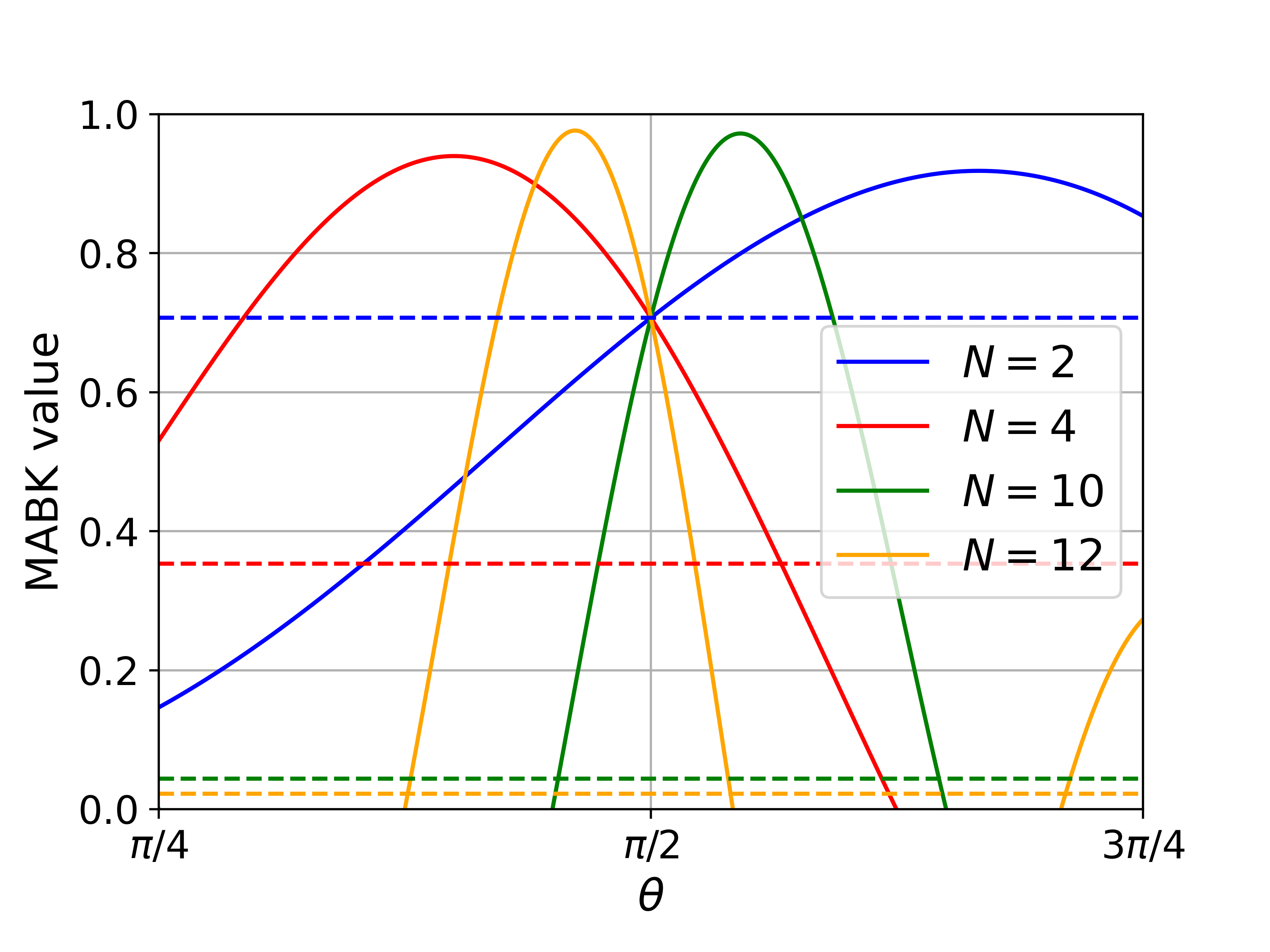
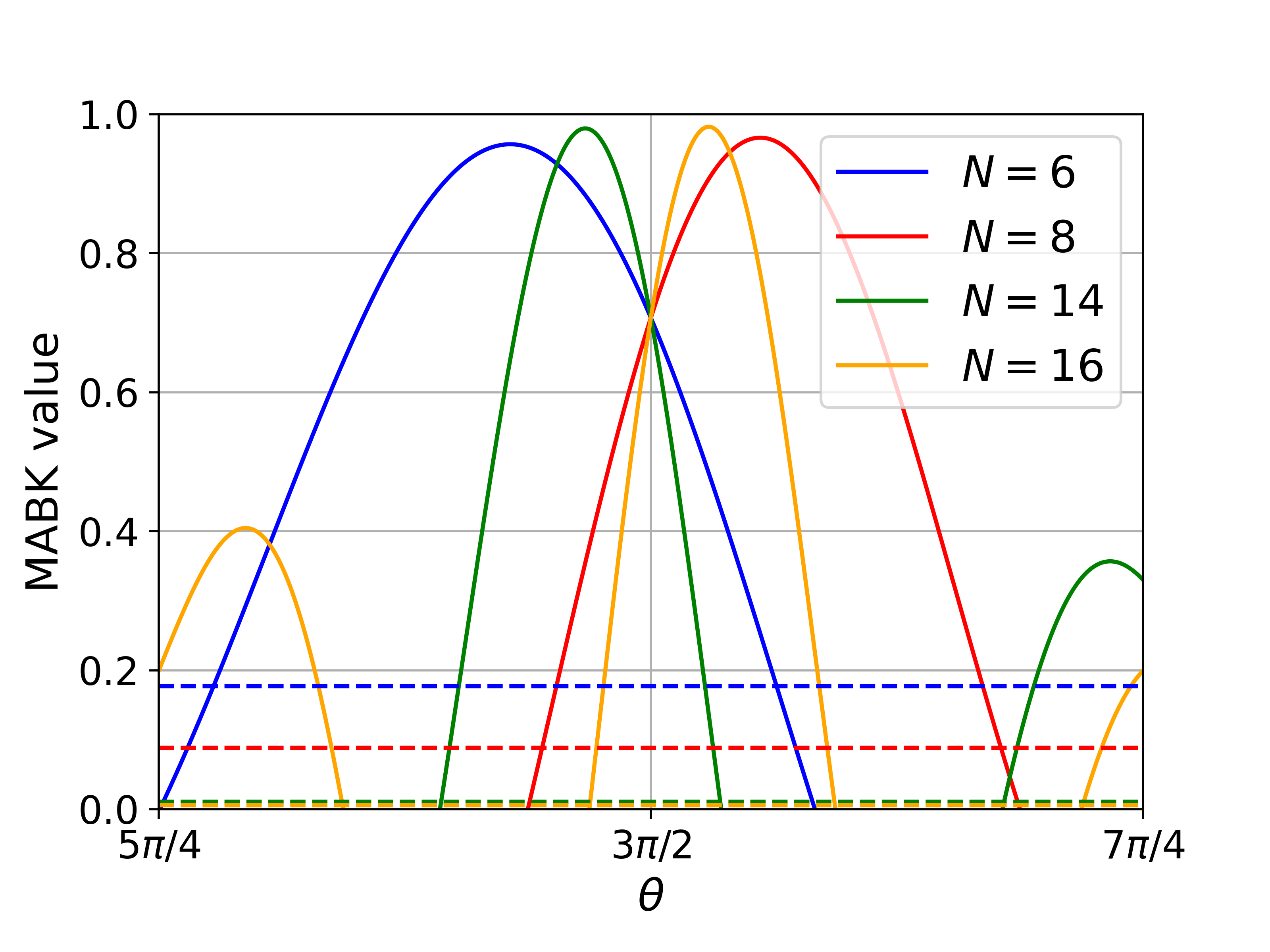
Figure 1: Using the family of strategies in (19) for even $N$ we plot the MABK value renormalized by the maximum quantum value over all strategies (i.e., $2^{(N-1)/2}$) in terms of $\theta\in[\pi/4,3\pi/4]$, and $\theta\in[5\pi/4,7\pi/4]$ respectively. The dashed lines indicate where the strategy becomes local. All points in this interval, excluding the boundaries and center point, correspond to strategies that certify $N$ bits of randomness device-independently using our expanded Bell expressions.

Due to Eq. 25, the MABK value $m_{N}^{*}$ becomes an achievable lower bound on the maximum MABK value for quantum correlations certifying maximum randomness. Part $(ii)$ of 1 says this is optimal, in the sense that one cannot achieve a larger MABK value whilst simultaneously certifying maximum randomness. As evidence we derive a numerical technique that can generate upper bounds on this question, and show these upper bounds match the lower bounds for some specific $N$. See Section B.3 for the details.

Finally, part $(iii)$ of 1 implies that when $N$ is odd, one can always achieve maximum randomness and any MABK value simultaneously. For the case of $\langle M_{N}\rangle=2^{(N-1)/2}$, i.e., the maximum quantum value, randomness can be certified according to Eq. 14. For all other MABK values, we conjecture maximum randomness can be certified by $I_{\theta}$ for some $\theta\in\mathcal{G}$. Evidence for this can be found in Fig. 2, where we plot the MABK value as a function of $\theta$ for different $N$, and see that maximal randomness is compatible with all nonlocal values of MABK that are achievable.

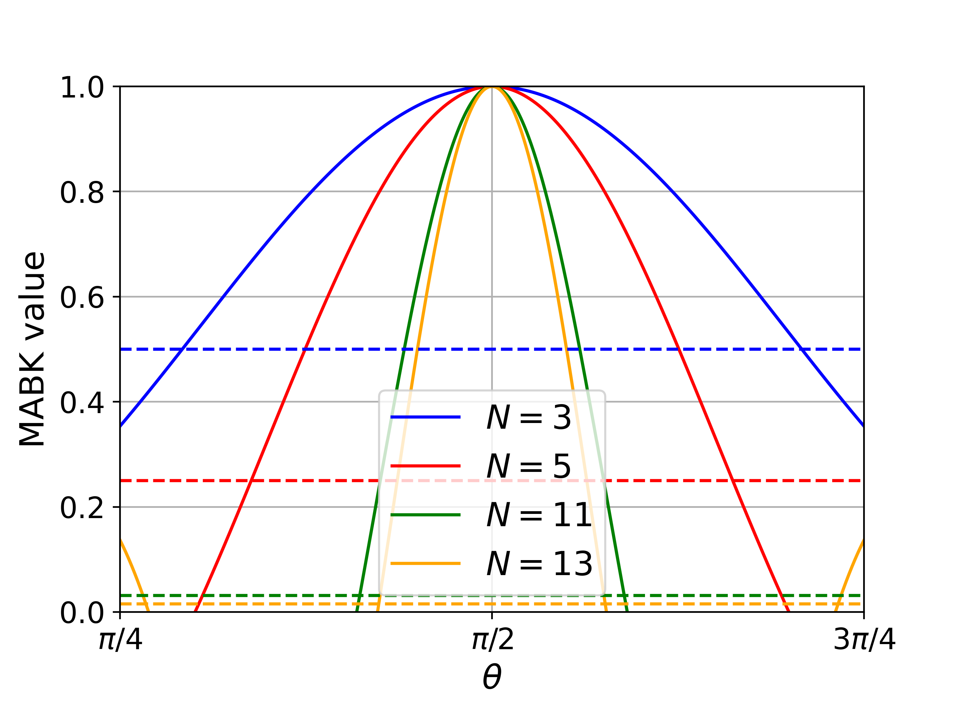
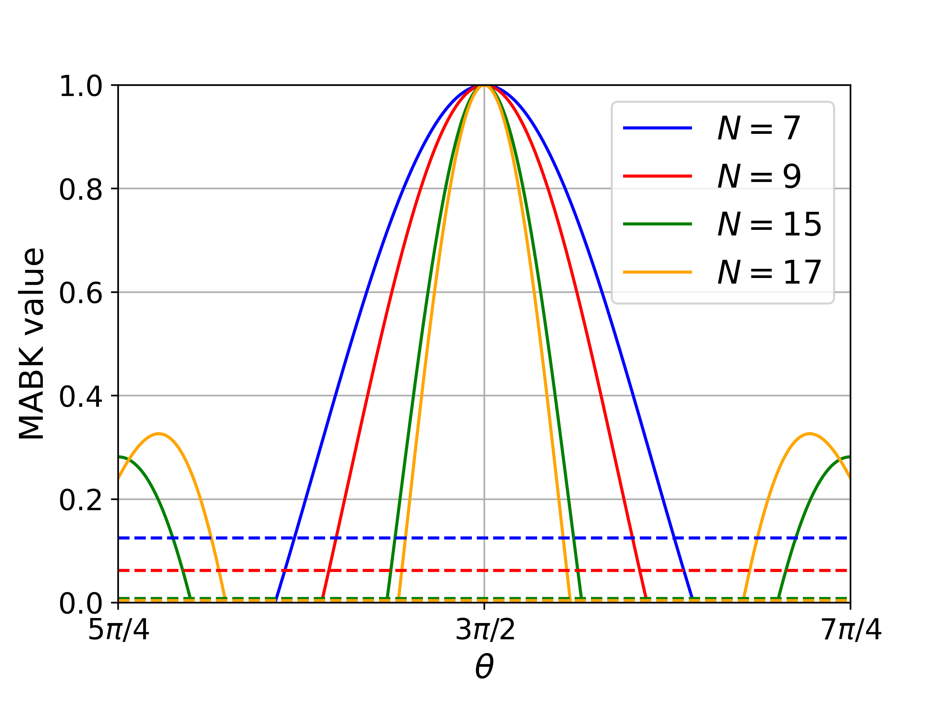
Figure 2: A similar plot to that of Fig. 1 for odd $N$ and second measurement angle of all parties $\theta\in[\pi/4,3\pi/4]$, and $\theta\in[5\pi/4,7\pi/4]$ respectively. All points in this interval, excluding the boundaries, correspond to strategies that can certify $N$ bits of randomness device-independently, using our expanded Bell expressions, or using the MABK inequality for the center points.

The discussion above leads to the further conjecture that, as was proven for the $N=2$ case Wooltorton et al. (2022); Acín et al. (2012), one can always achieve maximum randomness device-independently with correlations that lie arbitrarily close to the MABK facet of the local polytope. There is also a nontrivial maximal MABK violation for which this randomness is achievable when $N$ is even, unlike the odd case; as discussed in Section IV.1, this can be seen as a consequence of the $N$ even MABK expressions containing every $N$ party correlator. When maximum randomness is being certified, one of these correlators must be zero, which restricts the maximum MABK violation to be strictly less than the optimal quantum value.

IV.3.2 Asymptotic behaviour

We now consider the behaviour of the conjectured maximal MABK value achievable with maximum randomness, $m_{N}^{*}$ for increasingly large even $N$. We show that $m_{N}^{*}$ converges to the largest possible quantum value in this limit. Note this is not based on a conjecture; $m_{N}^{*}$ is an achievable lower bound, and in the following proposition we show this lower bound tends towards the global upper bound, namely the maximal quantum MABK value.

Proposition 4 (Maximum randomness in the asymptotic limit).

In the limit of large even $N$, one can achieve arbitrarily close to the maximum quantum violation of the $N$ party MABK inequality, $2^{(N-1)/2}$, whilst certifying maximum device-independent randomness.

This is proven in Section B.4.

IV.3.3 Nonlocality and maximum randomness

Whilst we have studied the MABK values achieved by the strategies in Eq. 19, we also consider how nonlocal they are, quantified by how much the local set needs to be “diluted” to contain them. We refer to this measure as the local dilution, which can be computed via a linear program (LP) for small $N$, and we give details in Section B.5. Our findings are presented in Fig. 3.

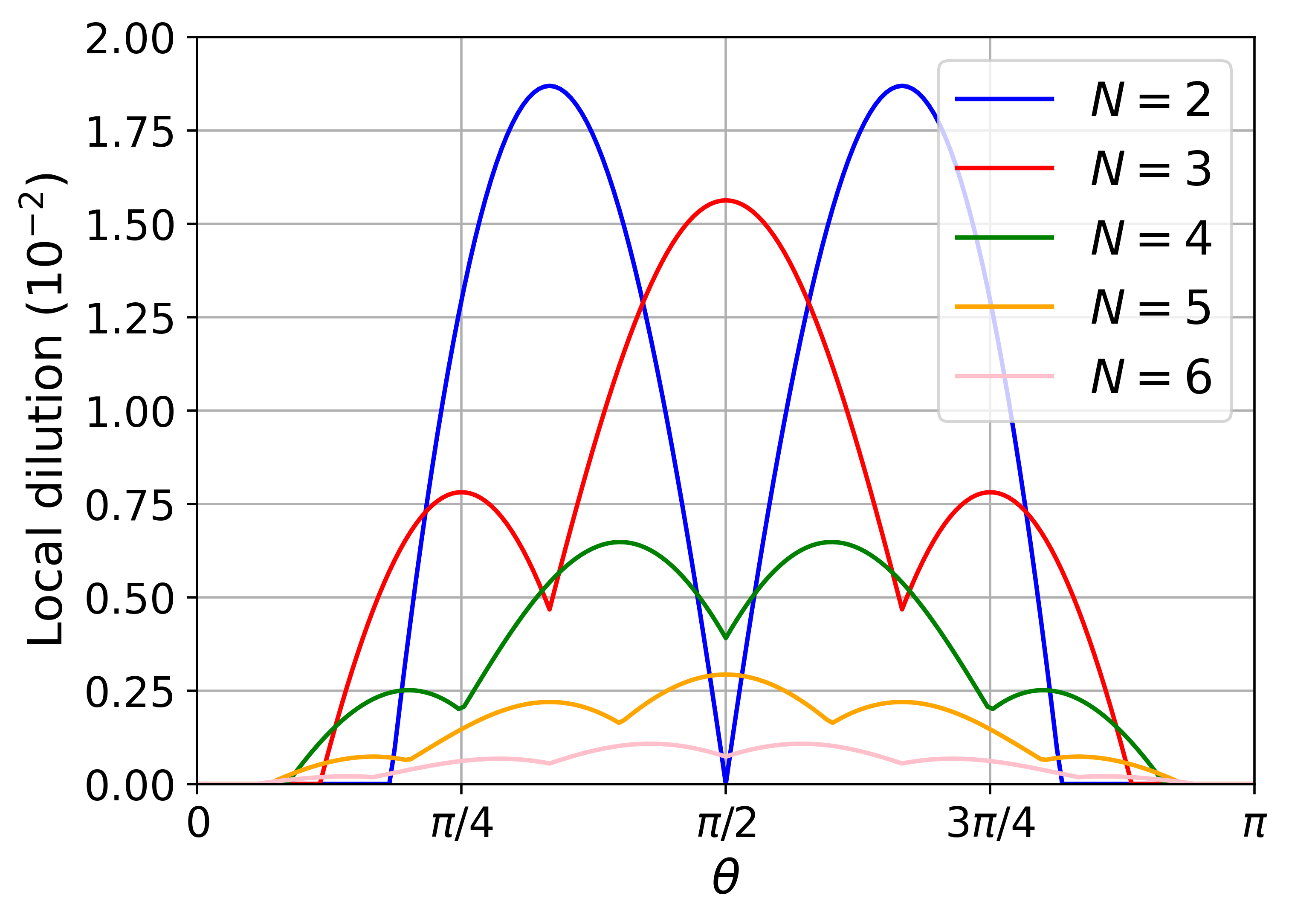
Figure 3: Nonlocality, as measured using local dilution, of the strategies in Eq. 19, for second measurement angle of all parties $\theta\in[0,\pi]$. All values of $\theta\in(\pi/4,\pi/2)\cup(\pi/2,3\pi/4)$ correspond to strategies which can certify $N$ bits of maximum randomness using our technique for expanding Bell expressions. $\theta=\pi/2$ can also correspond to maximum randomness when $N$ is odd by testing the MABK inequality.

Interestingly, for $N>2$ the correlations of the strategy in Eq. 19 are not close to the local boundary for any $\theta\in\mathcal{G}$, even for small MABK violation; whilst the violation of a given MABK inequality can be made arbitrarily small, the correlations are still distant from the local boundary. In fact, by comparing Fig. 3 with Fig. 1 and Fig. 2, one can see how correlations achieving at or below the maximum local MABK value, $\langle M_{N}\rangle\leq 1$, can still be nonlocal and certify maximum randomness. This is because the correlations violate some other Bell inequality, highlighting the complexity of randomness versus nonlocality in the multipartite scenario.

V Trade-off between DI randomness and MABK violation

In this section, we present an achievable lower bound on the maximum device-independent randomness that can be generated by correlations achieving any given MABK violation. Moreover, we conjecture this lower bound to be tight based on numerical evidence. This is achieved by introducing a new family of two parameter quantum strategies along with their self-testing Bell expressions. Using this as the seed, we construct a multipartite Bell expression which certifies their randomness.

V.1 Constructing the Bell expression

V.1.1 Bipartite self-tests

We begin by introducing a versatile family of bipartite self-tests which generalize the results in Wooltorton et al. (2022).

Lemma 7 ($J_{\phi,\theta}$ family of self-tests).

Let $(\phi,\theta)\in\mathbb{R}^{2}$ such that $\cos(2\theta)\cos(2\phi)<0$ and $\cos(\theta-\phi)\neq 0$. Define the family of Bell expressions parameterized by $\phi$ and $\theta$,

$$\langle J_{\phi,\theta}^{(k,l)}\rangle=\cos 2\theta\cos(\theta-\phi)\langle A_{0}^{(k)}A_{0}^{(l)}\rangle\\ -\cos 2\theta\cos 2\phi\big{(}\langle A_{0}^{(k)}A_{1}^{(l)}\rangle+\langle A_{1}^{(k)}A_{0}^{(l)}\rangle\big{)}\\ +\cos 2\phi\cos(\theta-\phi)\langle A_{1}^{(k)}A_{1}^{(l)}\rangle.$$ (27)

Then we have the following:

1. The local bounds are given by $\pm\eta_{\phi,\theta}^{\mathrm{L}}$, where

   $$\eta_{\phi,\theta}^{\mathrm{L}}=\max\big{\{}|\cos(\theta-\phi)(\cos 2\theta-\cos 2\phi)|,\\ |\cos(\theta-\phi)\big{(}\cos 2\theta+\cos 2\phi\big{)}|+|2\cos 2\phi\cos 2\theta|\big{\}}.$$ (28)

2. The quantum bounds are given by $\pm\eta_{\phi,\theta}^{\mathrm{Q}}$, where $\eta_{\phi,\theta}^{\mathrm{Q}}=2\sin^{2}(\theta+\phi)\sin(\theta-\phi)$.

3. Up to local isometries, there exists a unique strategy that achieves $\langle J_{\phi,\theta}^{(k,l)}\rangle=\eta_{\phi,\theta}^{\mathrm{Q}}$:

   $$\rho_{Q_{k}Q_{l}} =|\psi\rangle\!\langle\psi|,\ \mathrm{where}\ |\psi\rangle=\frac{1}{\sqrt{2}}\big{(}|00\rangle+i|11\rangle\big{)}$$ (29)

   $$A_{0}^{(k)} =A_{0}^{(l)}=\cos(\phi)\,\sigma_{X}-\sin(\phi)\,\sigma_{Y}$$

   $$A_{1}^{(k)} =A_{1}^{(l)}=\cos(\theta)\,\sigma_{X}+\sin(\theta)\,\sigma_{Y}.$$

Note that when $\phi=0$ Lemma 7 reduces to Lemma 4. Moreover, this Bell expression retains the same symmetry properties of the $I_{\theta}$ family, namely that $\langle J_{\phi,\theta}\rangle=-\eta^{\mathrm{Q}}_{\phi,\theta}$ for the state $|\psi^{\prime}\rangle$ and the same measurements, and is hence a self-test. We provide a full self-testing proof in Section B.6.

For future convenience, we define the set $\mathcal{F}=\Big{[}(-\pi/4,\pi/4)\times\mathcal{G}\Big{]}\cup\Big{[}(-\pi/4,\pi/4)\setminus\{0\}\times\{\pi/2,3\pi/2\}\Big{]}\subset\mathbb{R}^{2}$. One can verify that points $(\theta,\phi)\in\mathcal{F}$ satisfy $\sin^{2}(\theta+\phi)\geq\cos^{2}(\theta-\phi)$, and $\eta^{\mathrm{L}}_{\phi,\theta}<|\eta^{\mathrm{Q}}_{\phi,\theta}|$; i.e. they define a valid self-test according to Lemma 7.

V.1.2 Target strategy

For the $N$-partite case, we will consider the following strategy:

$$\begin{gathered}\rho_{\bm{Q}}=|\psi_{\mathrm{GHZ}}\rangle\!\langle\psi_{\mathrm{GHZ}}|\\ A_{0}^{(k)}=\cos\phi\,\sigma_{X}-\sin\phi\,\sigma_{Y},\\ A_{1}^{(k)}=\cos\theta\,\sigma_{X}+\sin\theta\,\sigma_{Y},\ k\in\{1,...,N\}.\end{gathered}$$ (30)

Using the fact that $\langle A_{\bm{x}}\rangle=\sin(n\theta-(N-n)\phi)$, where $n=\sum_{k}x_{k}$, the MABK value, defined in Eq. 1, of the above strategy is given by

$$\langle M_{N}(\phi,\theta)\rangle=2^{\frac{N-1}{2}}\Big{(}\cos^{N}\big{[}(\theta+\phi)/2+\pi/4\big{]}\\ \cdot\sin\big{[}N(\theta-\phi)/2+\pi/4\big{]}\\ +\cos^{N}\big{[}(\theta+\phi)/2-\pi/4\big{]}\sin\big{[}N(\theta-\phi)/2-\pi/4\big{]}\Big{)}.$$ (31)

V.1.3 Constructing an $N$-partite Bell inequality

Using the previous two building blocks, we construct the following Bell inequality using the $J_{\phi,\theta}$ expressions as the seed.

Lemma 8.

Let $\bm{\mu}$ be a tuple of $N-2$ measurement outcomes for all parties excluding $k,l$, and $n_{\bm{\mu}}\in\{0,1\}$ be the parity of $\bm{\mu}$. Let $(\phi^{\prime},\theta^{\prime})\in\mathcal{F}$ and $\{I_{\bm{\mu}}^{(k,l)}\}_{\bm{\mu}}$ be a set of bipartite Bell expressions between parties $k,l$, where

$$I_{\bm{\mu}}^{(k,l)}=(-1)^{n_{\bm{\mu}}}J_{\theta^{\prime},\phi^{\prime}}^{(k,l)}.$$ (32)

Then the expanded Bell expression given by

$$I_{\theta^{\prime},\phi^{\prime}}=\sum_{k=1}^{N-1}\Bigg{(}\sum_{\bm{\mu}}\tilde{P}^{\overline{(k,N)}}_{\bm{\mu}|\bm{0}}I_{\bm{\mu}}^{(k,N)}\Bigg{)}$$ (33)

has a quantum bound $\pm\eta_{N,\theta^{\prime},\phi^{\prime}}^{\mathrm{Q}}$ where $\eta_{N,\theta^{\prime},\phi^{\prime}}^{\mathrm{Q}}=2(N-1)\sin^{2}(\theta^{\prime}+\phi^{\prime})\sin(\theta^{\prime}-\phi^{\prime})$, achieved up to relabelings by the strategy in Eq. 30 by setting $\phi=-2\phi^{\prime}/(N-2)$ and $\theta=\theta^{\prime}+\phi^{\prime}$, and defines a nontrivial Bell inequality.

The proof is given in Section B.7. Note that the Bell expressions (33) are written in terms of the shifted parameters $(\phi^{\prime},\theta^{\prime})$, instead of the measurement angles $(\phi,\theta)$. This is because the $N-2$ parties performing the projection no longer use $\sigma_{X}$, but use $\cos(\phi)\,\sigma_{X}-\sin(\phi)\,\sigma_{Y}$. This accumulates a phase factor on the state of the remaining parties, $(|00\rangle+i(-1)^{n_{\bm{\mu}}}\exp\{i(N-2)\phi\}|11\rangle)/\sqrt{2}$, which is equivalent to the action of some local unitary $U$ on $(|00\rangle+i(-1)^{n_{\bm{\mu}}}|11\rangle)/\sqrt{2}$. To correct for this, we use the Bell expression $U^{\dagger}J_{\phi,\theta}^{(k,l)}U=J_{\phi^{\prime},\theta^{\prime}}^{(k,l)}$ as the seed. See Section B.7 for the exact calculation.

V.2 Randomness versus MABK value

Using the previously derived Bell inequality, we consider the trade-off between maximum device-independent randomness and MABK violation. Let us define

$$\theta(\phi)=\frac{N-1}{N+1}\phi+\theta^{*}_{N},$$ (34)

where $\theta_{N}^{*}$ is defined in Eq. 24 and also

$$\phi_{N}^{*}=\mathrm{sgn}[\sin(2\theta_{N}^{*})]\frac{\pi}{4N}.$$ (35)

For the strategy in Eq. 30, direct calculation yields

$$\langle M_{N}(\phi_{N}^{*},\theta(\phi_{N}^{*}))\rangle=2^{(N-1)/2},$$ (36)

and $\langle M_{N}(0,\theta(0))\rangle=m_{N}^{*}$. Hence by varying $\phi\in[0,\phi_{N}^{*}]$ and choosing $\theta=\theta(\phi)$ one can obtain the desired range of MABK values $[m_{N}^{*},2^{(N-1)/2}]$, from the conjectured maximum MABK value with maximum randomness to the maximum quantum value. Choosing this parameterization, the raw randomness, $H(\bm{R}|\bm{X}=\bm{x}^{*})=H(\{p_{\phi}(\bm{a}|\bm{0})\})$, of the strategy in Eq. 30, as a function of $\phi$, is given by

$$H(\{p_{\phi}(\bm{a}|\bm{0})\})\equiv r(\phi)=N-1+H_{\mathrm{bin}}\Big{[}\frac{1-\sin N\phi}{2}\Big{]},$$ (37)

where $H_{\mathrm{bin}}$ is the binary entropy function and $r(\phi)$ is a smooth, monotonically decreasing function of $\phi$ in the range $[0,\phi_{N}^{*}]$.

As shown in Section IV, when $\phi=0$ we can certify maximum DI randomness. It also follows from the self-testing properties of the MABK family that when $\phi=\phi^{*}_{N}$ we obtain $N-1+3/2-\log_{2}(1+\sqrt{2})/\sqrt{2}\approx N-0.4$ bits of global DI randomness. What remains then, is to apply the new Bell expression constructed in Lemma 8 to certify $r(\phi)$ bits of DI randomness for $\phi\in(0,\phi^{*}_{N})$. To do so, the following proposition shows that for every $\phi\in[0,\phi_{N}^{*}]$, there exists a valid Bell expression given by Lemma 8.

Proposition 5.

Let $\phi\in[0,\phi_{N}^{*}]$, and define $\phi^{\prime}=-(N-2)\phi/2$, $\theta^{\prime}=\theta(\phi)-\phi^{\prime}$. Then $(\phi^{\prime},\theta^{\prime})\in\mathcal{F}$, where $\mathcal{F}$ is defined in Lemma 7.

This is proven in Section B.8. Proposition 5 implies that, for every $\phi$ in the range we are interested in, the bipartite expression $(-1)^{n_{\bm{\mu}}}J_{\phi^{\prime},\theta^{\prime}}$ is a valid self-test of the strategy

$$\rho_{Q_{k}Q_{l}} =|\Phi_{\bm{\mu}}\rangle\!\langle\Phi_{\bm{\mu}}|,$$ (38)

$$A_{0}^{(k)} =A_{0}^{(l)}=\cos\phi^{\prime}\,\sigma_{X}-\sin\phi^{\prime}\,\sigma_{Y}$$

$$A_{1}^{(k)} =A_{1}^{(l)}=\cos\theta^{\prime}\,\sigma_{X}+\sin\theta\,\sigma_{Y}.$$

After applying the local unitary $U_{\phi}\otimes U_{\phi}$, where $U_{\phi}=|0\rangle\!\langle 0|+e^{-i(N-2)\phi/2}|1\rangle\!\langle 1|$, this is equivalent to

$$\rho_{Q_{k}Q_{l}} =|\Phi_{\bm{\mu},\phi}\rangle\!\langle\Phi_{\bm{\mu},\phi}|,$$ (39)

$$A_{0}^{(k)} =A_{0}^{(l)}=\cos\phi\,\sigma_{X}-\sin\phi\,\sigma_{Y}$$

$$A_{1}^{(k)} =A_{1}^{(l)}=\cos\theta\,\sigma_{X}+\sin\theta\,\sigma_{Y},$$

which is exactly the bipartite strategy we wanted to self-test, since it is the one held by parties $k$ and $N$ after the projector $\tilde{P}_{\bm{\mu}|\bm{0}}^{\overline{(k,N)}}$ is applied to the global state $|\psi_{\mathrm{GHZ}}\rangle$. As a result, the correlations generated by the strategy in Eq. 30, by setting $\theta=\theta(\phi)$ and varying $\phi\in[0,\phi_{N}^{*}]$, maximally violate the Bell inequality $I_{\theta^{\prime},\phi^{\prime}}$ with $\phi^{\prime}=-(N-2)\phi/2$ and $\theta^{\prime}=\theta(\phi)-\phi^{\prime}$. We can therefore employ the decoupling lemma to make the rate unconditioned on Eve, $r(\phi)$, device-independent.

Proposition 6.

Achieving the maximum quantum value of the Bell inequality in Lemma 8 certifies $r(\phi)$ bits of randomness, i.e.

$$R_{I_{\theta^{\prime},\phi^{\prime}}}(\eta^{\mathrm{Q}}_{N,\theta^{\prime},\phi^{\prime}})=r(\phi).$$ (40)

We have established, for every MABK value $s\in[m_{N}^{*},2^{(N-1)/2}]$, that there exists a $\phi_{s}\in[0,\phi_{N}^{*}]$ which defines a quantum strategy achieving $s$, for which its generated randomness $r(\phi_{s})$ is device-independent. We have therefore related every MABK value with a DI rate. We conjecture the curve $(s,r(\phi_{s}))$ is optimal in terms of raw randomness, which can then be made device-independent following the above discussion — see Lemma 9.

Conjecture 2.

For $N$ even, the maximum randomness unconditioned on Eve, $r$, that can be generated by quantum strategies achieving an MABK value, $s$, is given by

$$r(s)=\begin{cases}N,\ s\in(1,m_{N}^{*}],\\ r(\phi_{s}),\ s\in(m_{N}^{*},2^{(N-1)/2}],\end{cases}$$ (41)

where $r(\phi)$ is defined in Eq. 37, and

$$\phi_{s}=\mathrm{arg\,min}\big{\{}|\phi|\ :\ \phi\in[0,\phi_{N}^{*}],\langle M_{N}(\phi,\theta(\phi))\rangle=s\big{\}}.$$ (42)

For the range $s\in(1,m_{N}^{*}]$, and $s\in(m_{N}^{*},2^{(N-1)/2}]$, the rate $r(s)$ and MABK value $s$ is achieved by the family of quantum strategies in Eq. 19 and Eq. 30, and certified by the Bell expressions in Lemma 5 and Lemma 8, respectively.

The minimization in the definition of $\phi_{s}$ is included since we have not shown the set $\{\ \phi\in[0,\phi_{N}^{*}]\ :\ \langle M_{N}(\phi,\theta(\phi))\rangle=s\}$ is unique. Intuitively, the closer $\phi_{s}$ is to zero the closer we are to maximum randomness; hence we expect $r(\phi)$ to be monotonically decreasing with $|\phi|$ for $\phi\in[0,\phi_{N}^{*}]$, and minimisation guarantees the best rate at a given $s$. For the examples we have computed, the minimization turns out to be trivial, i.e. over a single point.

Lemma 9.

Suppose 1 and Eq. 42 hold. Then the maximum amount of device-independent randomness that can be certified for the range of Mermin values $(1,2^{(N-1)/2}]$ is given by Eq. 41.

The above lemma tells us that if the rate in Eq. 41 is optimal without conditioning on Eve, it will also be optimal conditioned on Eve, i.e., the rate can be made device-independent. This is because Eqs. 25 and 5 ensure that, for every MABK value, the corresponding quantum strategy achieving it, given in Eq. 19 or Eq. 30, can generate certifiable randomness using the corresponding Bell expression $I_{\theta}$ or $I_{\theta^{\prime},\phi^{\prime}}$. A rewriting of Lemma 9 without Conjectures 1 and 42, would say that (41) corresponds to a guaranteed lower bound on the maximum DI randomness as a function of MABK value. Our results are summarized in Fig. 4.

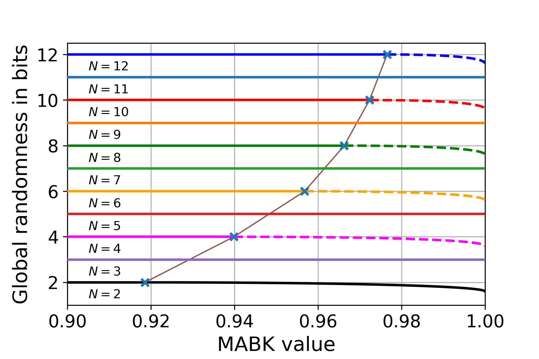
Figure 4: The conjectured curves of maximum device-independent randomness versus MABK value, where the MABK value is normalized by its maximum quantum value $2^{(N-1)/2}$. When $N$ is odd, maximum global randomness can be achieved for any MABK value between the local and quantum bound, indicated by solid lines. The blue crosses indicate the conjectured maximum MABK value for which maximum randomness can be achieved when $N$ is even, $m_{N}^{*}$, which tends towards the maximum quantum value as $N\rightarrow\infty$. To the left of the blue crosses, $N$ bits of randomness can be achieved for MABK values between the local bound (not shown on this axis) and $m_{N}^{*}$; since this is the global maximum, it is optimal, indicated by solid lines. To the right of the blue crosses, dashed lines indicate lower bounds on the trade-off between maximum randomness and MABK value from $m_{N}^{*}$ to the maximum quantum value, which are conjectured to be tight. The case of $N=2$ was proven in Ref Wooltorton et al. (2022), which we reproduce with our results.

We provide evidence for Conjectures 1 and 42 in Section B.9, where we derive a numerical technique for upper bounding the maximum randomness that can be generated by quantum strategies achieving a given MABK value $s$. By studying the numerical results, we find our analytical lower bound closely agrees with the numerical upper bound.

V.3 Other extremal Bell inequalities

In the $N$-partite 2-input 2-output scenario, the MABK family is just one class of extremal Bell inequalities, and the techniques developed in this section can be readily applied to others. For example, when $N=3$, there are a total of 3 non-trivial, new classes, one being the MABK inequality $M_{3}$, and two being of the form Werner and Wolf (2001)

$$S_{1} =\frac{1}{4}\sum_{x,y,z}A_{x}B_{y}C_{z}-A_{1}B_{1}C_{1},$$ (43)

$$S_{2} =A_{0}B_{0}(C_{0}+C_{1})-A_{1}B_{1}(C_{0}-C_{1}),$$ (44)

where we have swapped $A_{x_{1}}^{(1)}$ with $A_{x}$ etc. for legibility. $S_{1}$ and $S_{2}$ have local bounds of $1$ and $2$, and maximum quantum values $5/3$ and $2\sqrt{2}$, respectively. We applied our numerical technique (see Section B.9) to find upper bounds on the maximum amount of randomness certifiable whilst achieving a given violation of $S_{1}$ and $S_{2}$. A comparison can be found in Fig. 5, and we provide additional figures and details in Section B.10.

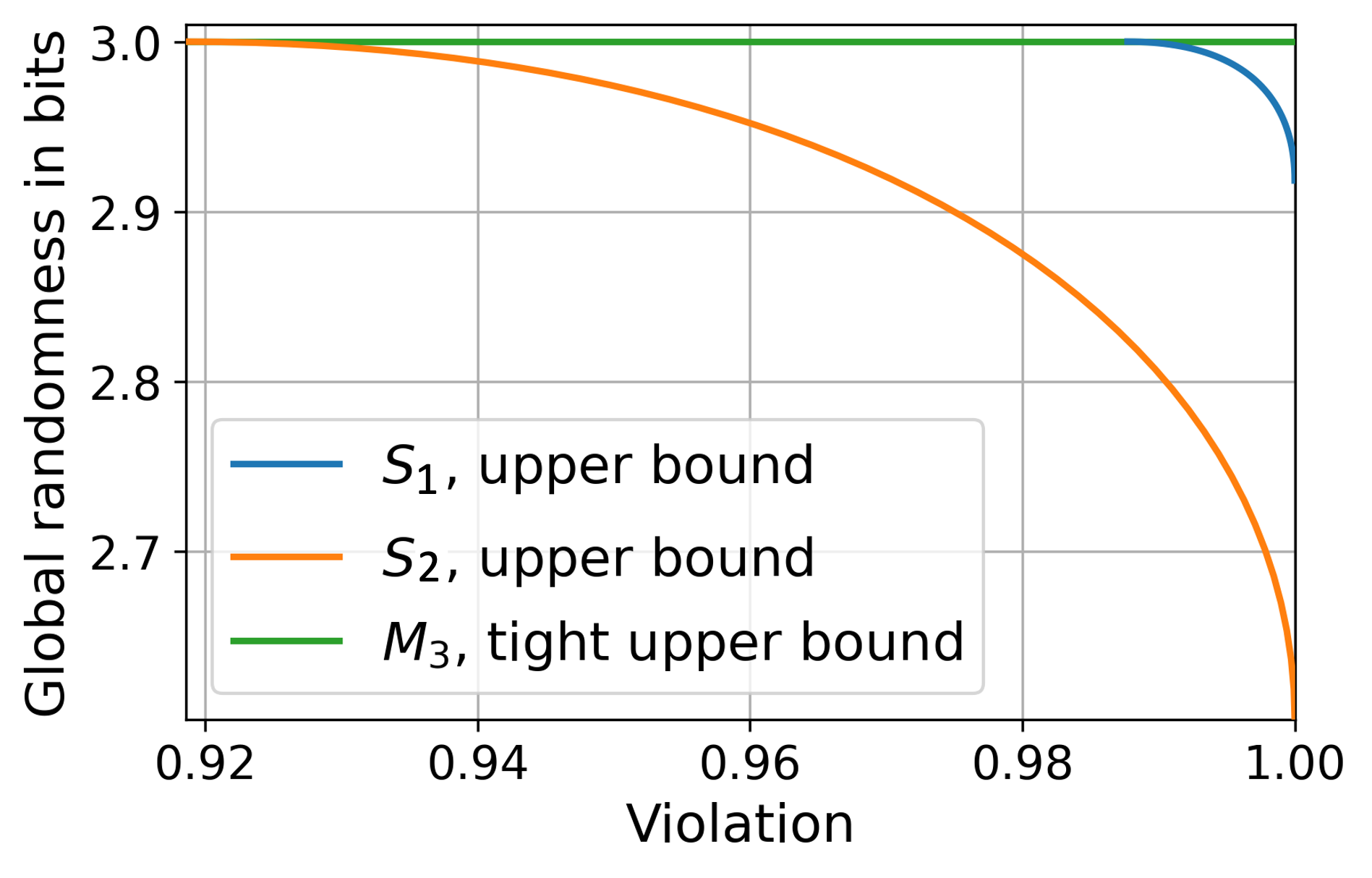
Figure 5: Upper bounds on the trade-off between asymptotic global DI randomness and violation of non-trivial extremal Bell inequalities, for the tripartite scenario with two binary measurements per party. The violation has been normalized by the maximum quantum value. $S_{1}$ and $S_{2}$ are given by Eq. 43 and Eq. 44 respectively, and $M_{3}$ is the MABK expression. Note the above graph does not necessarily imply a weaker trade-off for $S_{1}$, since the local bounds differ for all expressions once normalized by the maximum quantum value.

We find both $S_{1}$ and $S_{2}$ exhibit a trade-off for violations close to the quantum maximum. Due to its structure, $S_{2}$ exhibits identical trade-off characteristics to the CHSH inequality found in Wooltorton et al. (2022), with the maximum CHSH value achievable with maximum randomness being numerically close to $3\sqrt{3}/2$. On the other hand, we find more randomness can be generated from maximum violation of $S_{2}$, which is still strictly less than the maximum certified by MABK. Exact values are given in Section B.10.

VI Discussion

In this work, we studied how MABK violation constrains the generation of global DI randomness for an arbitrary number of parties. Whilst there is no trade-off in the odd case, we conjectured the precise trade-off for the even case. This conjecture is supported by an analytical lower bound and a numerical upper bound that agree up to several decimal places and have been checked for up to $N=12$. We additionally showed that, in the asymptotic limit, this trade-off vanishes. Our first technical contribution was the advancement of a recent tool, originally introduced to witness genuinely multipartite nonlocality, to randomness certification. Our second was the introduction of a new, versatile family of bipartite Bell expressions which generalizes some that were previously known.

More precisely, we discussed that odd MABK expressions contain half the full party correlators; considering input combinations not included in the Bell expression, we find some of these can be uniform. For even $N$, all correlators are included and must be non-zero to ascertain maximum violation, resulting in a trade-off. The number of correlators is $2^{N}$, whereas the quantum bound is $2^{(N-1)/2}$. Maximum violation is achieved when the product of all correlators and their MABK coefficients have the same value, which in this case will be $2^{-(N+1)/2}$. Hence we find the penalty for fixing one correlator to zero (which is necessary for maximum randomness) diminishes as $N$ grows, and vanishes in the asymptotic limit.

We also quantified the nonlocality of our constructions for low values of $N$, calculated via a linear program. Interestingly we found our correlations are always separated from the local boundary. It would be interesting to find correlations that lie asymptotically close to the local boundary whilst still certifying maximum randomness, as was found in the $N=2$ case Acín et al. (2012); Wooltorton et al. (2022). This could entail symmetry breaking between the second measurements of each party, and the versatility of the techniques presented here can be easily applied. Moreover, one could hope to go further and bound the trade-off between randomness and nonlocality in this setting; however, the challenge becomes finding a suitable measure of nonlocality that is efficient to work with.

We hope that the results found here will inform future experiments in DIRE; initial works have already made progress in this direction Seguinard et al. (2023). In such experiments, one should consider the optimal protocol for DIRE. In this work, we have proposed protocols that rely on spot-checking Miller and Shi (2014, 2017); Bhavsar et al. (2021), where randomness is generated by a single input combination. An alternative approach has been explored in reference Bhavsar et al. (2021), where it was found that generating randomness from all inputs and averaging the result boosts the rate when the CHSH inequality is used. For the noiseless scenario, spot-checking will always be optimal when a specific input combination leads to maximum randomness, as is the case in this work; having one maximally random setting necessarily implies that at least one other setting combination will not be maximally random for the correlations to be nonlocal, hence averaging will only decrease the overall rate. The noisy case remains an open question however, and the trade-off between using spot-checking and weighted averaging for our constructions deserves future investigation, with the aim of further improving practical rates.

Another interesting direction for future research is to connect expanded Bell inequalities to multipartite self-testing. Our decoupling result allows the structure of the post-measurement state to be certified following the maximum violation of an expanded Bell expression; the open question we pose is if an expanded Bell inequality can constitute a full self-test, opening up a new range of useful applications beyond randomness certification. Intuitively, if each pair of parties can self-test all of their measurements along with a projected state, one might hope to use the marginal information to make a statement about the global state. Such a strategy has already been adopted for self-testing multipartite correlations Šupić et al. (2018). However, there are subtleties. For example, for three parties with observables $A_{x},B_{y},C_{z}$, our first Bell expression in Eq. 21 when $\theta=\pi/2$, reads

$$A_{0}\big{(}B_{0}C_{1}+B_{1}C_{0}\big{)}+B_{0}\big{(}A_{0}C_{1}+A_{1}C_{0}\big{)}\leq_{\mathcal{Q}}4\mathbb{I},$$ (45)

which is achievable classically. This originates from the classical achievability of the seed $I_{\theta=\pi/2}^{(k,l)}=A_{0}^{(k)}A_{1}^{(l)}+A_{1}^{(k)}A_{0}^{(l)}$ in Eq. 16. Yet, the Bell expression was designed for the strategy

$$\begin{gathered}\rho_{Q_{A}Q_{B}Q_{C}}=|\psi_{\mathrm{GHZ}}\rangle\!\langle\psi_{\mathrm{GHZ}}|,\\ A_{0/1}=B_{0/1}=C_{0/1}=\sigma_{X/Y},\end{gathered}$$ (46)

which maximally violates the $N=3$ MABK inequality, and is known to be self-testing. In other words, when any party measures $\sigma_{X}$ or $\sigma_{Y}$ on $|\psi_{\mathrm{GHZ}}\rangle$, the resulting bipartite correlations are classical, even though the global strategy is nonlocal. It is then necessary to add extra measurements to enable bipartite self-testing. On the other hand, the $N=3$ MABK expression reads

$$A_{0}\big{(}B_{0}C_{1}+B_{1}C_{0}\big{)}+A_{1}\big{(}B_{0}C_{0}-B_{1}C_{1}\big{)}\leq_{\mathcal{Q}}4\mathbb{I},$$ (47)

which holds similarities to Eq. 45. Both terms in the sum are achievable classically, given by a relabeling of the seed $I_{\theta=\pi/2}^{(k,l)}$; the key difference is the lack of simultaneous classical achievability in Eq. 47. Clearly this property is sufficient. It would be interesting to understand if the $N=3$ MABK expression can still be viewed as an expansion of the seed $I_{\theta=\pi/2}^{(k,l)}$ following an appropriate relabelling, using only the strategy in Eq. 46 as the starting point. Note however, for $N>3$, we can use the $N=3$ MABK expression as the self-testing seed, and we do not run into this situation. Thus, correlations that do not exhibit post-measurement nonlocality, yet are still nonlocal, could be viewed as a resource to construct richer correlations.

Finally, whilst we studied the MABK family of inequalities, one could consider a similar analysis for other families of extremal multipartite Bell expressions Werner and Wolf (2001). For example, we explored upper bounds on the trade-offs for all extremal inequalities when $N=3$, and found the MABK inequality to be optimal for global randomness; it would be interesting to find out if the upper bounds presented for the other inequalities are achievable. One might try to find explicit constructions that match these bounds, and use our techniques to make them device-independent. Analysing other extremal inequalities will build a more complete picture of how DI randomness can be generated in the multipartite scenario, better informing the way forward for future multipartite experiments.

Appendix A Proofs for expanded Bell expressions

A.1 Proof of Lemma 1

Lemma 1. Let $I$ be an expanded Bell expression according to Footnote 1. The maximum quantum value of $\langle I\rangle$ is upper bounded by $\eta^{\mathrm{Q}}_{N}:=\sum_{k,l}c_{k,l}\eta^{\mathrm{Q}}$.

Proof.

To prove the above, we show that the operator expression $\bar{I}=\eta^{\mathrm{Q}}_{N}\mathbb{I}-I$ is non-negative. Since each bipartite expression satisfies $\langle I_{\bm{\mu}}^{(k,l)}\rangle\leq\eta^{\mathrm{Q}}$ for all $\bm{\mu},k,l$, we have positive expressions

$$\bar{I}_{\bm{\mu}}^{(k,l)}=\eta^{\mathrm{Q}}\mathbb{I}-I_{\bm{\mu}}^{(k,l)}\succeq 0,\ \forall\bm{\mu},k,l.$$ (48)

We then have

$$\bar{I}_{k,l} =\eta^{\mathrm{Q}}\mathbb{I}-\sum_{\bm{\mu}}\tilde{P}_{\bm{\mu}|\bm{0}}^{\overline{(k,l)}}I^{(k,l)}_{\bm{\mu}}$$

$$=\sum_{\bm{\mu}}\tilde{P}_{\bm{\mu}|\bm{0}}^{\overline{(k,l)}}\Big{(}\eta^{\mathrm{Q}}\mathbb{I}-I_{\bm{\mu}}^{(k,l)}\Big{)}$$

$$=\sum_{\bm{\mu}}\tilde{P}_{\bm{\mu}|\bm{0}}^{\overline{(k,l)}}\bar{I}_{\bm{\mu}}^{(k,l)}\succeq 0.$$ (49)

Finally it follows from the above that $\bar{I}\succeq 0$, which proves the upper bound on the maximum quantum value. We can also upper bound the maximum local value by $\sum_{k<l}c_{k,l}\eta^{\mathrm{L}}<\sum_{k<l}c_{k,l}\eta^{\mathrm{Q}}=\eta_{N}^{\mathrm{Q}}$ since $\eta^{\mathrm{L}}<\eta^{\mathrm{Q}}$. ∎

A.2 Uniqueness of binary distributions with fixed marginals

Before proving Eq. 12, we establish the following fact about classical distributions of bit strings when their conditional distributions are fixed. We will later use this result to justify that the distribution used for randomness achieving the quantum bound of an expanded Bell inequality is unique when the seed is a self-test.

Lemma 10.

Let $\bm{A}=A_{1}...A_{N}$, $N\geq 3$, be a random $N$ bit string which takes values $\bm{a}\in\{0,1\}^{N}$ according to the distribution $p_{\bm{A}}(\bm{a})$. Let $\bm{B}_{\bar{k}}$ be an $N-2$ bit partition of the string $\bm{A}$, excluding bits $N$ and $k\in\{1,...,N-1\}$, taking values $\bm{b}_{\bar{k}}\in\{0,1\}^{N-2}$. Then the distribution $p_{\bm{A}}(\bm{a})$ is entirely determined by the set of conditional distributions $\{p_{A_{k}A_{N}|\bm{B}_{\bar{k}}}(a_{k}a_{N}|\bm{b}_{\bar{k}})\}_{k\in\{1,...,N-1\}}$, provided $p_{A_{k}A_{N}|\bm{B}_{\bar{k}}}(a_{k}a_{N}|\bm{b}_{\bar{k}})>0$ for all $k,a_{k},a_{N},\bm{b}_{\bar{k}}$.

Proof.

Proof can be established using a recursive argument to solve for a set of marginal terms $p_{\bm{B}_{\bar{l}}}(\bm{b}_{\bar{l}})$, for a fixed $l\in\{1,...,N-1\}$, from which the full distribution can be recovered. Let us choose another partition $k\in\{1,...,N-1\}$ with $k\neq l$. Then we have

$$p_{\bm{A}}(\bm{a}) =p_{\bm{B}_{\bar{k}}}(\bm{b}_{\bar{k}})p_{A_{k}A_{N}|\bm{B}_{\bar{k}}}(a_{k}a_{N}|\bm{b}_{\bar{k}})$$ (50)

$$=p_{\bm{B}_{\bar{l}}}(\bm{b}_{\bar{l}})p_{A_{l}A_{N}|\bm{B}_{\bar{l}}}(a_{l}a_{N}|\bm{b}_{\bar{l}}).$$

By choosing different values of $a_{k}$, this implies the two sets of equations

$$p_{\bm{B}_{\bar{k}}}(\bm{b}_{\bar{k}}) p_{A_{k}A_{N}|\bm{B}_{\bar{k}}}(a_{k}=0,a_{N}|\bm{b}_{\bar{k}})$$ (51)

$$=p_{\bm{B}_{\bar{l}}}(a_{k}=0,\bm{b}_{\bar{kl}})p_{A_{l}A_{N}|\bm{B}_{\bar{l}}}(a_{l}a_{N}|a_{k}=0,\bm{b}_{\bar{kl}}),$$

$$p_{\bm{B}_{\bar{k}}}(\bm{b}_{\bar{k}}) p_{A_{k}A_{N}|\bm{B}_{\bar{k}}}(a_{k}=1,a_{N}|\bm{b}_{\bar{k}})$$

$$=p_{\bm{B}_{\bar{l}}}(a_{k}=1,\bm{b}_{\bar{kl}})p_{A_{l}A_{N}|\bm{B}_{\bar{l}}}(a_{l}a_{N}|a_{k}=1,\bm{b}_{\bar{kl}}).$$

Since $p_{A_{k}A_{N}|\bm{B}_{\bar{k}}}(a_{k}a_{N}|\bm{b}_{\bar{k}})\neq 0$, we can rearrange both for $p_{\bm{B}_{\bar{k}}}$ and equate:

$$\frac{p_{\bm{B}_{\bar{l}}}(a_{k}=0,\bm{b}_{\bar{kl}})p_{A_{l}A_{N}|\bm{B}_{\bar{l}}}(a_{l}a_{N}|a_{k}=0,\bm{b}_{\bar{kl}})}{p_{A_{k}A_{N}|\bm{B}_{\bar{k}}}(a_{k}=0,a_{N}|\bm{b}_{\bar{k}})}\\ =\frac{p_{\bm{B}_{\bar{l}}}(a_{k}=1,\bm{b}_{\bar{kl}})p_{A_{l}A_{N}|\bm{B}_{\bar{l}}}(a_{l}a_{N}|a_{k}=1,\bm{b}_{\bar{kl}})}{p_{A_{k}A_{N}|\bm{B}_{\bar{k}}}(a_{k}=1,a_{N}|\bm{b}_{\bar{k}})},$$ (52)

where we have explicitly written in the $a_{k}$ variable, and $\bar{kl}$ denotes a tuple excluding parties $k$ and $l$. The above equation tells us, for every choice of $\bm{b}_{\bar{kl}}\in\{0,1\}^{N-3}$, the unknowns $p_{\bm{B}_{\bar{l}}}(a_{k}=0,\bm{b}_{\bar{kl}})$ and $p_{\bm{B}_{\bar{l}}}(a_{k}=1,\bm{b}_{\bar{kl}})$ are linearly dependent. Hence we consider the $2^{N-3}$ unknowns $p_{\bm{B}_{\bar{l}}}(a_{k}=0,\bm{b}_{\bar{kl}})$, since the $a_{k}=1$ terms can be computed via this linear dependence.

Consider choosing $k^{\prime}\in\{1,...,N-1\}\setminus\{k,l\}$. We can find a new set of equations by repeating the above process with $k^{\prime}$ instead of $k$, to find:

$$\frac{p_{\bm{B}_{\bar{l}}}(a_{k}=0,a_{k^{\prime}}=0,\bm{b}_{\overline{kk^{\prime}l}})}{p_{A_{k^{\prime}}A_{N}|\bm{B}_{\bar{k^{\prime}}}}(a_{k^{\prime}}=0,a_{N}|a_{k}=0,\bm{b}_{\overline{kk^{\prime}}})}$$ (53)

$$\hskip 22.76228pt\cdot p_{A_{l}A_{N}|\bm{B}_{\bar{l}}}(a_{l}a_{N}|a_{k}=0,a_{k^{\prime}}=0,\bm{b}_{\overline{kk^{\prime}l}})$$

$$=\frac{p_{\bm{B}_{\bar{l}}}(a_{k}=0,a_{k^{\prime}}=1,\bm{b}_{\overline{kk^{\prime}l}})}{p_{A_{k^{\prime}}A_{N}|\bm{B}_{\bar{k^{\prime}}}}(a_{k^{\prime}}=1,a_{N}|a_{k}=0,\bm{b}_{\overline{kk^{\prime}}})}$$

$$\hskip 22.76228pt\cdot p_{A_{l}A_{N}|\bm{B}_{\bar{l}}}(a_{l}a_{N}|a_{k}=0,a_{k^{\prime}}=1,\bm{b}_{\overline{kk^{\prime}l}}),$$

where we have only included the $a_{k}=0$ case, and written $\overline{kk^{\prime}l}$ to denote a tuple excluding parties $k,k^{\prime},l$. Notice we have now identified linear dependence between $p_{\bm{B}_{\bar{l}}}(a_{k}=0,a_{k^{\prime}}=0,\bm{b}_{\overline{kk^{\prime}l}})$ and $p_{\bm{B}_{\bar{l}}}(a_{k}=0,a_{k^{\prime}}=1,\bm{b}_{\overline{kk^{\prime}l}})$. None of these equations contain a marginal with $a_{k}=1$, so they relate pairs of unknowns distinctly to the parings from the previous equations, and are hence linearly independent. As before, we can proceed with the $2^{N-4}$ unknowns $p_{\bm{B}_{\bar{l}}}(a_{k}=0,a_{k^{\prime}}=0,\bm{b}_{\overline{kk^{\prime}l}})$ and recover the others by linear dependence.

We can apply the above procedure iteratively a total of $N-2$ times (for every $k\in\{1,...,N-1\}\setminus\{l\}$), halving the number of unknowns on every iteration by establishing linear dependence. Starting with $2^{N-2}$ marginals $p_{\bm{B}_{\bar{l}}}(\bm{b}_{\overline{l}})$, this leaves us with 1 unknown, which can be solved via normalization, completing the proof. ∎

Now we can present a corollary which will be needed for the proof of Eq. 12, showing the conditional distribution used for randomness, $p(\bm{a}|\bm{0})$, achieving the quantum bound of an expanded Bell expression is unique.

Corollary 1.

Let $I$ be an expanded Bell inequality according to Footnote 1 with $c_{k,N}=1$ if $k<N$ and zero otherwise, and $\eta_{N}^{\mathrm{Q}}$ defined in Lemma 1. Let $I$ be constructed using a seed with the self-testing properties described in Eq. 12, and $p(\bm{a}|\bm{x})$ denote a quantum behaviour that achieves $\langle I\rangle=\eta^{\mathrm{Q}}_{N}$. Then provided $p(a_{k}a_{N}|\bm{b}_{\bar{k}},\bm{x}=\bm{0})>0$ for all $k,a_{k},a_{N},\bm{b}_{\bar{k}}$, the conditional the distribution $p(\bm{a}|\bm{0})$ is unique.

Proof.

If the quantum value $\langle I\rangle=\eta_{N}^{\mathrm{Q}}$ is achieved, we must have

$$\sum_{k=1}^{N-1}\big{\langle}\eta^{\mathrm{Q}}\mathbb{I}-\sum_{\bm{\mu}}\tilde{P}_{\bm{\mu}|\bm{0}}^{\overline{(k,N)}}I_{\bm{\mu}}^{(k,N)}\big{\rangle}=0,$$ (54)

which implies $\big{\langle}\eta^{\mathrm{Q}}\mathbb{I}-\sum_{\bm{\mu}}\tilde{P}_{\bm{\mu}|\bm{0}}^{\overline{(k,N)}}I_{\bm{\mu}}^{(k,N)}\big{\rangle}=0$ from Eq. 49. Next we apply Hölder’s inequality:

$$\langle\tilde{P}_{\bm{\mu}|\bm{0}}^{\overline{(k,N)}}I_{\bm{\mu}}^{(k,N)}\rangle\\ \leq\|\tilde{P}_{\bm{\mu}|\bm{0}}^{\overline{(k,N)}}\rho_{\bm{Q}E}\tilde{P}_{\bm{\mu}|\bm{0}}^{\overline{(k,N)}}\|_{1}\|I_{\bm{\mu}}^{(k,N)}\|_{\infty}=\langle\tilde{P}_{\bm{\mu}|\bm{0}}^{\overline{(k,N)}}\rangle\eta^{\mathrm{Q}},$$ (55)

where $\rho_{\bm{Q}E}=|\Psi\rangle\!\langle\Psi|$, $|\Psi\rangle$ is the quantum state that realizes the correlations and identities on $E$ are implicit. Since

$$\sum_{\bm{\mu}}\Big{(}\langle\tilde{P}_{\bm{\mu}|\bm{0}}^{\overline{(k,N)}}\rangle\eta^{\mathrm{Q}}-\langle\tilde{P}_{\bm{\mu}|\bm{0}}^{\overline{(k,N)}}I_{\bm{\mu}}^{(k,N)}\rangle\Big{)}=0$$ (56)

we conclude $\langle\tilde{P}_{\bm{\mu}|\bm{0}}^{\overline{(k,N)}}I_{\bm{\mu}}^{(k,N)}\rangle=\langle\tilde{P}_{\bm{\mu}|\bm{0}}^{\overline{(k,N)}}\rangle\eta^{\mathrm{Q}}$. Now we can write

$$\langle\Psi^{\prime}|I_{\bm{\mu}}^{(k,N)}|\Psi^{\prime}\rangle=\eta_{Q},$$ (57)

where we define the normalized state $|\Psi^{\prime}\rangle=\tilde{P}_{\bm{\mu}|\bm{0}}^{\overline{(k,N)}}|\Psi\rangle/\sqrt{\langle\tilde{P}_{\bm{\mu}|\bm{0}}^{\overline{(k,N)}}\rangle}$. The self-testing properties of $I_{\bm{\mu}}^{(k,N)}$ (see definition in Eq. 12) then determine the unique correlations $\langle\Psi^{\prime}|\tilde{P}_{a_{k}|0}^{(k)}\tilde{P}_{a_{N}|0}^{(N)}|\Psi^{\prime}\rangle=p^{k,N}_{\bm{\mu}}(a_{k}a_{N}|xy)$. Using the definition of $|\Psi^{\prime}\rangle$, we find

$$\big{\langle}\tilde{P}_{\bm{\mu}|\bm{0}}^{\overline{(k,N)}}\tilde{P}_{a_{k}|0}^{(k)}\tilde{P}_{a_{N}|0}^{(N)}\big{\rangle}=\langle\tilde{P}_{\bm{\mu}|\bm{0}}^{\overline{(k,N)}}\rangle p^{k,N}_{\bm{\mu}}(a_{k}a_{N}|00).$$ (58)

We can now directly apply Corollary 1. Explicitly we have $p_{\bm{A}}(\bm{a})=\big{\langle}\tilde{P}_{\bm{\mu}|\bm{0}}^{\overline{(k,N)}}\tilde{P}_{a_{k}|0}^{(k)}\tilde{P}_{a_{N}|0}^{(N)}\big{\rangle}$, and the $N-1$ fixed conditional distributions $p_{A_{k}A_{N}|\bm{B}_{\bar{k}}}(a_{k}a_{l}|\bm{b}_{\bar{k}})=p(a_{k}a_{N}|\bm{b}_{\bar{k}},\bm{x}=\bm{0})=p^{k,N}_{\bm{\mu}}(a_{k}a_{N}|00)$, where we have identified $\bm{\mu}=\bm{b}_{\bar{k}}$.

∎

A.3 Proof of Eq. 12

We can now proceed to prove Eq. 12 in the main text, which is restated below:

Lemma 2. Let $I$ be an expanded $N$-party Bell expression defined in Footnote 1 with binary inputs and outputs, and $c_{k,N}=1$ if $k<N$ and zero otherwise. Suppose for every $I_{\bm{\mu}}^{(k,N)}$, there exists an SOS decomposition which self-tests the same pure bipartite entangled state $|\Phi\rangle$ between parties $k,N$, along with some ideal measurements $P^{(k)}_{a_{k}|x_{k}},P^{(N)}_{a_{N}|x_{N}}$, according to Eq. 2, which satisfy $\langle\Phi|P^{(k)}_{a_{k}|0}\otimes P^{(N)}_{a_{N}|0}|\Phi\rangle>0$ for all $a_{k},a_{N}$. Then for any strategy $|\Psi\rangle_{\tilde{\bm{Q}}E},\big{\{}\{\tilde{P}_{a_{k}|x_{k}}^{(k)}\}_{x_{k}}\big{\}}_{k}$ that achieves $\langle I\rangle=\eta^{\mathrm{Q}}_{N}$, the post-measurement state $\rho_{\bm{R}E}$, for measurement settings $\bm{x}=\bm{0}$, admits the tensor product decomposition,

$$\rho_{\bm{R}E|\bm{0}}=\rho_{\bm{R}|\bm{0}}\otimes\rho_{E}.$$ (59)

Proof.

We will break this proof up into four steps. First, we will provide an SOS decomposition for the Bell operator $\bar{I}$, and derive the algebraic constraints satisfied by any state and measurements that achieves its maximum value. These turn out to be those implied by the bipartite bell expressions that build up $I$. Next, we will employ Jordan’s lemma, reducing the problem to qubits, and show how these constraints self-test the bipartite states. Finally we write down the global post-measurement state, and show how these self-tests imply a tensor product with $E$.

A.3.1 SOS decomposition

We begin by introducing SOS decompositions for the bipartite Bell operators,

$$\bar{I}_{\bm{\mu}}^{(k,N)}=\sum_{i}M_{\bm{\mu},i}^{(k,N)\dagger}M_{\bm{\mu},i}^{(k,N)},$$ (60)

where $M_{\bm{\mu},i}^{(k,N)}$ is a polynomial of the operators $A_{x_{k}}^{(k)}$, $A_{x_{N}}^{(N)}$. We now use this to build an SOS decomposition for $\bar{I}$,

$$\bar{I} =\sum_{k=1}^{N-1}\bar{I}_{k,l}$$

$$=\sum_{k=1}^{N-1}\sum_{\bm{\mu}}\tilde{P}_{\bm{\mu}|\bm{0}}^{\overline{(k,N)}}\bar{I}_{\bm{\mu}}^{(k,N)}$$

$$=\sum_{k=1}^{N-1}\sum_{\bm{\mu}}\sum_{i}\Big{(}\tilde{P}_{\bm{\mu}|\bm{0}}^{\overline{(k,N)}}M_{\bm{\mu},i}^{(k,N)}\Big{)}^{\dagger}\Big{(}\tilde{P}_{\bm{\mu}|\bm{0}}^{\overline{(k,N)}}M_{\bm{\mu},i}^{(k,N)}\Big{)}.$$ (61)

Now, for some physical state $|\Psi\rangle$ and observables, observation of the maximum quantum value, $\langle\bar{I}\rangle=0$, immediately implies the algebraic constraints

$$\tilde{P}_{\bm{\mu}|\bm{0}}^{\overline{(k,N)}}M_{\bm{\mu},i}^{(k,N)}|\Psi\rangle=0,\ \forall k\in\{1,...,N-1\},\bm{\mu},i.$$ (62)

Since $\tilde{P}_{\bm{\mu}|\bm{0}}^{\overline{(k,N)}}$ and $M_{\bm{\mu},i}^{(k,N)}$ commute, we define the post-measurement states

$$|\Psi_{\bm{\mu},k}\rangle=\frac{\tilde{P}_{\bm{\mu}|\bm{0}}^{\overline{(k,N)}}|\Psi\rangle}{\sqrt{\langle\Psi|\tilde{P}_{\bm{\mu}|\bm{0}}^{\overline{(k,N)}}|\Psi\rangle}},$$ (63)

and arrive at the set of algebraic constraints, for a fixed $k,\bm{\mu}$,

$$M_{\bm{\mu},i}^{(k,N)}|\Psi_{\bm{\mu},k}\rangle=0,\quad\forall i.$$ (64)

A.3.2 Applying Jordan’s lemma

Next, we employ Jordan’s lemma, which allows us to reduce our analysis to a convex combination of $N$-qubit systems. We write $\mathcal{H}_{Q_{k}}$ to denote the qubit Hilbert space of party $k$, and introduce a flag system $\mathcal{H}_{F_{k}}$ which indicates the block. Then for every party $\mathcal{H}_{\tilde{Q}_{k}}=\mathcal{H}_{Q_{k}}\otimes\mathcal{H}_{F_{k}}$, and the purified state takes the form

$$|\Psi\rangle_{\tilde{\bm{Q}}E}=\sum_{\bm{f}}\sqrt{p_{\bm{f}}}|\bm{f}\rangle_{\bm{F}}\otimes|\varphi^{\bm{f}}\rangle_{\bm{Q}E}\otimes|\bm{f}\rangle_{E^{\prime}},$$ (65)

where $\rho^{\bm{f}}=\mathrm{Tr}_{E}\big{[}|\varphi^{\bm{f}}\rangle\!\langle\varphi^{\bm{f}}|\big{]}$ is an $N$-qubit state corresponding to block $\bm{f}=(f_{1},...,f_{N})$, where $f_{k}$ indexes the block for party $k$ and $p_{\bm{f}}>0$ form a probability distribution. Tracing out $EE^{\prime}$, the total state received by the parties is then a convex combination of qubit states, and Eve holds a purification of the state in register $E$ along with a label in register $E^{\prime}$ telling her which block it pertains to. Similarly, the projectors decompose

$$\tilde{P}_{a_{k}|x_{k}}^{(k)}=\sum_{f_{k}}|f_{k}\rangle\!\langle f_{k}|_{F_{k}}\otimes P_{a_{k}|x_{k}}^{(f_{k})},$$ (66)

where $P_{a_{k}|x_{k}}^{(f_{k})}$ is a rank one single qubit projector on $\mathcal{H}_{Q_{k}}$ corresponding to block $f_{k}$ Jordan (1875); Pironio et al. (2009); Bhavsar et al. (2021).

$$\tilde{P}_{\bm{\mu}|\bm{0}}^{\overline{(k,N)}}=\sum_{\bm{f}_{(\overline{k,N})}}|\bm{f}_{(\overline{k,N})}\rangle\!\langle\bm{f}_{(\overline{k,l})}|_{\bm{F}_{(\overline{k,N})}}\otimes P_{\bm{\mu}|\bm{0}}^{(\bm{f}_{(\overline{k,N})})},$$ (67)

where the notation $(\overline{k,N})$ is understood to denote a tuple excluding entries $k,N$, e.g. $\bm{f}_{(\overline{k,N})}$ is a tuple of indices $f_{k^{\prime}}$ for $k^{\prime}\neq k,N$. $P_{\bm{\mu}|\bm{0}}^{(\bm{f}_{(\overline{k,N})})}=\bigotimes_{k^{\prime}\neq k,N}P^{(f_{k^{\prime}})}_{\mu_{k^{\prime}}|0}$ is then a rank one projector on the $N-2$ qubit Hilbert space shared by all parties excluding $k$ and $N$, corresponding to the block $\bm{f}_{(\overline{k,N})}$.

We can now apply Jordan’s lemma to the projected states $|\Psi_{\bm{\mu},k}\rangle$, by computing

$$|\Psi_{\bm{\mu},k}\rangle =\sum_{\bm{f}}\sqrt{p_{\bm{f}}}|\bm{f}\rangle_{\bm{F}}$$

$$\ \ \ \ \otimes\frac{\Big{(}\mathbb{I}_{Q_{k}Q_{N}E}\otimes P_{\bm{\mu}|\bm{0}}^{(\bm{f}_{(\overline{k,N})})}\Big{)}|\varphi^{\bm{f}}\rangle_{\bm{Q}E}}{\sqrt{\langle\Psi|\tilde{P}_{\bm{\mu}|\bm{0}}^{\overline{(k,N)}}|\Psi\rangle}}\otimes|\bm{f}\rangle_{E^{\prime}}$$

$$=\sum_{\bm{f}\in S_{\bm{\mu}}^{k}}\sqrt{p_{\bm{f}}}|\bm{f}\rangle_{\bm{F}}\otimes|\phi_{\bm{\mu}}^{\bm{f}_{(\overline{k,N})}}\rangle_{\bm{Q}_{(\overline{k,N})}}$$

$$\ \ \ \ \ \ \ \ \otimes|\psi_{\bm{\mu},k}^{\bm{f}}\rangle_{Q_{k}Q_{N}E}\otimes|\bm{f}\rangle_{E^{\prime}}$$ (68)

where $S_{\bm{\mu}}^{k}\ni\bm{f}$ is the set of blocks for which the projection is non-zero. Here $\bm{f}$ is understood to be the concatenation of $f_{k},f_{N},\bm{f}_{(\overline{k,N})}$, and we used the fact that the qubit projectors are rank one to write the state as a tensor product,

$$\frac{\Big{(}\mathbb{I}_{Q_{k}Q_{N}E}\otimes P_{\bm{\mu}|\bm{0}}^{(\bm{f}_{(\overline{k,N})})}\Big{)}|\varphi^{\bm{f}}\rangle_{\bm{Q}E}}{\sqrt{\langle\Psi|\tilde{P}_{\bm{\mu}|\bm{0}}^{\overline{(k,N)}}|\Psi\rangle}}\\ =\begin{cases}|\phi_{\bm{\mu}}^{\bm{f}_{(\overline{k,N})}}\rangle_{\bm{Q}_{(\overline{k,N})}}\otimes|\psi_{\bm{\mu},k}^{\bm{f}}\rangle_{Q_{k}Q_{N}E}\ \mathrm{if}\ \bm{f}\in S_{\bm{\mu}}^{k},\\ 0\ \mathrm{otherwise},\end{cases}$$ (69)

where $|\phi_{\bm{\mu}}^{\bm{f}_{(\overline{k,N})}}\rangle=\bigotimes_{k^{\prime}\neq k,N}|\phi_{\mu_{k^{\prime}}}^{f_{k^{\prime}}}\rangle$, and $|\phi_{\mu_{k^{\prime}}}^{f_{k^{\prime}}}\rangle$ spans the support of $P^{(f_{k^{\prime}})}_{\mu_{k^{\prime}}|0}$. $|\psi_{\bm{\mu},k}^{\bm{f}}\rangle_{Q_{k}Q_{l}E}$ is then the state held by parties $k,N$ and Eve following the projection. By writing $|\tilde{\phi}_{\bm{\mu}}^{\bm{f}_{(\overline{k,N})}}\rangle_{\tilde{\bm{Q}}_{{(\overline{k,N})}}}=|\bm{f}_{(\overline{k,N})}\rangle_{\bm{F}_{(\overline{k,N})}}\otimes|\phi_{\bm{\mu}}^{\bm{f}_{(\overline{k,N})}}\rangle_{\bm{Q}_{{(\overline{k,N})}}}$, and $|\tilde{\psi}_{\bm{\mu},k}^{\bm{f}}\rangle_{\tilde{Q}_{k}\tilde{Q}_{N}E}=|f_{k}f_{N}\rangle_{F_{k}F_{N}}\otimes|\psi_{\bm{\mu},k}^{\bm{f}}\rangle_{Q_{k}Q_{N}E}$, we can re-write the constraints in Eq. 64 as

$$\sum_{\bm{f}\in S_{\bm{\mu}}^{k}}\sqrt{p_{\bm{f}}}|\tilde{\phi}_{\bm{\mu}}^{\bm{f}_{(\overline{k,N})}}\rangle_{\tilde{\bm{Q}}_{{(\overline{k,N})}}}\\ \otimes M_{\bm{\mu},i}^{(k,N)}|\tilde{\psi}_{\bm{\mu},k}^{\bm{f}}\rangle_{\tilde{Q}_{k}\tilde{Q}_{N}E}\otimes|\bm{f}\rangle_{E^{\prime}}=0,$$ (70)

implying, for a fixed $k,\bm{\mu}$,

$$M_{\bm{\mu},i}^{(k,N)}|\tilde{\psi}_{\bm{\mu},k}^{\bm{f}}\rangle_{\tilde{Q}_{k}\tilde{Q}_{N}E}=0,\ \forall i,\forall\bm{f}\in S_{\bm{\mu}}^{k}.$$ (71)

A.3.3 Applying the bipartite self-tests

For the next part of the proof, we use the self-testing properties of the bipartite Bell expression $I^{(k,l)}_{\bm{\mu}}$, which are in turn derived from the SOS polynomials, and the constraints they impose on any state which achieves the maximum quantum value. Explicitly, for any state which satisfies the polynomial constraints, there exists a local isometery which transforms that state into an ideal state in tensor product with some junk. Due to Jordan’s lemma, the constraints in Eq. 71 certify the the existence of a local unitary on parties $k$ and $N$, for every measurement outcome $\bm{\mu}$ and block combination $\bm{f}\in S_{\bm{\mu}}^{k}$, $U_{\bm{\mu},k}^{\bm{f}}$, that satisfies for some fixed two qubit state $|\Phi\rangle$ and projectors $P_{a_{k}|x_{k}}^{(k)}$, $P_{a_{N}|x_{N}}^{(N)}$,

$$\Big{(}\mathbb{I}_{F_{k}F_{N}}\otimes U_{\bm{\mu},k}^{\bm{f}}\otimes\mathbb{I}_{E}\Big{)}\Big{(}\tilde{P}_{a_{k}|x_{k}}^{(k)}\otimes\tilde{P}_{a_{N}|x_{N}}^{(N)}\Big{)}|\tilde{\psi}_{\bm{\mu},k}^{\bm{f}}\rangle_{\tilde{Q}_{k}\tilde{Q}_{N}E}\\ =|f_{k}f_{N}\rangle_{F_{k}F_{N}}\otimes\Big{(}P_{a_{k}|x_{k}}^{(k)}\otimes P_{a_{N}|x_{N}}^{(N)}\Big{)}|\Phi\rangle_{Q_{k}Q_{N}}\otimes|\lambda_{\bm{\mu},k}^{\bm{f}}\rangle_{E},$$ (72)

where $|\lambda_{\bm{\mu},k}^{\bm{f}}\rangle_{E}$ is the junk system left over in the Eve register, which a priori may depend on $\bm{\mu},k$. Recall we required that all bipartite expressions self-test the same state up to local unitaries, hence the above equation holds for all $\bm{\mu}$.

A.3.4 Global post-measurement state

Finally, we use the existence of local unitaries $U_{\bm{\mu},k}^{\bm{f}}$ to analyse the global post-measurement state held by all parties following their zero measurement, which takes the form

$$\rho_{\bm{R}EE^{\prime}|\bm{0}}=\sum_{a_{k},a_{N},\bm{\mu}}|a_{k}a_{N}\bm{\mu}\rangle\!\langle a_{k}a_{N}\bm{\mu}|_{\bm{R}}\otimes\\ \mathrm{Tr}_{\tilde{\bm{Q}}}\Big{[}\Big{(}\tilde{P}_{a_{k}|0}^{(k)}\otimes\tilde{P}_{a_{N}|0}^{(N)}\otimes\tilde{P}_{\bm{\mu}|\bm{0}}^{\overline{(k,N)}}\otimes\mathbb{I}_{EE^{\prime}}\Big{)}|\Psi\rangle\!\langle\Psi|\Big{]}.$$ (73)

We can rewrite the term inside the partial trace

$$\Big{(}\tilde{P}_{a_{k}|0}^{(k)}\otimes\tilde{P}_{a_{N}|0}^{(N)}\otimes\tilde{P}_{\bm{\mu}|\bm{0}}^{\overline{(k,N)}}\otimes\mathbb{I}_{EE^{\prime}}\Big{)}|\Psi\rangle$$

$$=\sqrt{\langle\Psi|\tilde{P}_{\bm{\mu}|\bm{0}}^{\overline{(k,N)}}|\Psi\rangle}\Big{(}\tilde{P}_{a_{k}|0}^{(k)}\otimes\tilde{P}_{a_{N}|0}^{(N)}\otimes\mathbb{I}_{\tilde{\bm{Q}}_{(\overline{k,N})}}\otimes\mathbb{I}_{EE^{\prime}}\Big{)}|\Psi_{\bm{\mu},k}\rangle$$

$$=\sqrt{\langle\Psi|\tilde{P}_{\bm{\mu}|\bm{0}}^{\overline{(k,N)}}|\Psi\rangle}\sum_{\bm{f}\in S_{\bm{\mu}}^{k}}\sqrt{p_{\bm{f}}}|\tilde{\phi}_{\bm{\mu}}^{\bm{f}_{(\overline{k,N})}}\rangle_{\tilde{\bm{Q}}_{{(\overline{k,N})}}}$$

$$\ \ \ \ \ \ \ \ \otimes\Big{(}\tilde{P}_{a_{k}|0}^{(k)}\otimes\tilde{P}_{a_{N}|0}^{(N)}\Big{)}|\tilde{\psi}_{\bm{\mu},k}^{\bm{f}}\rangle_{\tilde{Q}_{k}\tilde{Q}_{N}E}\otimes|\bm{f}\rangle_{E^{\prime}}$$

$$=\sqrt{\langle\Psi|\tilde{P}_{\bm{\mu}|\bm{0}}^{\overline{(k,N)}}|\Psi\rangle}\sum_{\bm{f}\in S_{\bm{\mu}}^{k}}\sqrt{p_{\bm{f}}}|\tilde{\phi}_{\bm{\mu}}^{\bm{f}_{(\overline{k,N})}}\rangle_{\tilde{\bm{Q}}_{{(\overline{k,N})}}}$$

$$\otimes|f_{k}f_{N}\rangle_{F_{k}F_{N}}\otimes U_{\bm{\mu},k}^{\bm{f}\dagger}\Big{(}P_{a_{k}|0}^{(k)}\otimes P_{a_{N}|0}^{(N)}\Big{)}|\Phi\rangle_{Q_{k}Q_{N}}$$

$$\ \ \ \ \ \ \ \ \otimes|\lambda_{\bm{\mu},k}^{\bm{f}}\rangle_{E}\otimes|\bm{f}\rangle_{E^{\prime}}.$$ (74)

Now, tracing out $\tilde{\bm{Q}}$ equates to tracing out systems $\bm{F}\bm{Q}$, which yields

$$\mathrm{Tr}_{\tilde{\bm{Q}}}\Big{[}\Big{(}\tilde{P}_{a_{k}|0}^{(k)}\otimes\tilde{P}_{a_{N}|0}^{(N)}\otimes\tilde{P}_{\bm{\mu}|\bm{0}}^{\overline{(k,N)}}\otimes\mathbb{I}_{EE^{\prime}}\Big{)}|\Psi\rangle\!\langle\Psi|\Big{]}$$

$$=\langle\Psi|\tilde{P}_{\bm{\mu}|\bm{0}}^{\overline{(k,N)}}|\Psi\rangle\langle\Phi|\Big{(}P_{a_{k}|0}^{(k)}\otimes P_{a_{N}|0}^{(N)}\Big{)}|\Phi\rangle$$

$$\ \ \ \ \ \ \ \ \cdot\sum_{\bm{f}\in S_{\bm{\mu}}^{k}}p_{\bm{f}}|\lambda_{\bm{\mu},k}^{\bm{f}}\rangle\!\langle\lambda_{\bm{\mu},k}^{\bm{f}}|_{E}\otimes|\bm{f}\rangle\!\langle\bm{f}|_{E^{\prime}}.$$ (75)

By employing Corollary 1, we know that, following observation of $\langle I\rangle=\eta^{\mathrm{Q}}$, the marginals $\langle\Psi|\tilde{P}_{\bm{\mu}|\bm{0}}^{\overline{(k,l)}}|\Psi\rangle$ are unique; hence the following equality holds:

$$\langle\Psi|\tilde{P}_{\bm{\mu}|\bm{0}}^{\overline{(k,N)}}|\Psi\rangle\langle\Phi|\Big{(}P_{a_{k}|0}^{(k)}\otimes P_{a_{N}|0}^{(N)}\Big{)}|\Phi\rangle=p(a_{k},a_{N},\bm{\mu}|\bm{0}),$$ (76)

where $\{p(a_{k},a_{N},\bm{\mu}|\bm{0})\}_{a_{k},a_{N},\bm{\mu}}$ are those unique correlations needed to achieve $\langle I\rangle=\eta^{\mathrm{Q}}$. We then find

$$\rho_{\bm{R}EE^{\prime}|\bm{0}}=\sum_{a_{k},a_{N},\bm{\mu}}p(a_{k},a_{N},\bm{\mu}|\bm{0})|a_{k}a_{N}\bm{\mu}\rangle\!\langle a_{k}a_{N}\bm{\mu}|_{\bm{R}}\\ \otimes\sum_{\bm{f}\in S_{\bm{\mu}}^{k}}p_{\bm{f}}|\lambda^{\bm{f}}_{\bm{\mu},k}\rangle\!\langle\lambda^{\bm{f}}_{\bm{\mu},k}|_{E}\otimes|\bm{f}\rangle\!\langle\bm{f}|_{E^{\prime}}.$$ (77)

Now notice, Eve can still establish correlations with the $N$ parties excluding $k$ and $N$, by choosing the sets $\{S_{\bm{\mu}}^{k}\}_{\bm{\mu}}$ to be disjoint. She could then distinguish the different outcomes $\bm{\mu}$ by a projective measurement on $E^{\prime}$. She can also establish correlations by making the set $\{|\lambda^{\bm{f}}_{\bm{\mu},k}\rangle\}_{\bm{\mu}}$ distinguishable and measuring $E$. To show Eve is in fact uncorrelated with all parties, we use the fact that there are $N-1$ choices of $k$, i.e. one can choose different combinations of parties to maximally violate the bipartite self-tests.

We now include extra notation $\overline{kN}$, $\bm{\mu}\rightarrow\bm{\mu}_{\overline{kN}}$, which denotes a tuple of $N-2$ outcomes for all parties excluding $k$ and $N$, and define the following state, which is just a rewriting of Eq. 77 making the choice $k$ explicit:

$$\rho_{\bm{R}EE^{\prime}|\bm{0}}^{k}:=\sum_{a_{k},a_{N},\bm{\mu}_{\overline{kN}}}p(a_{k},a_{N},\bm{\mu}_{\overline{kN}}|\bm{0})\\ \cdot|a_{k}a_{N}\bm{\mu}_{\overline{kN}}\rangle\!\langle a_{k}a_{N}\bm{\mu}_{\overline{kN}}|_{\bm{R}}\\ \otimes\sum_{\bm{f}\in S_{\bm{\mu}_{\overline{kN}}}^{k}}p_{\bm{f}}|\lambda^{\bm{f}}_{\bm{\mu}_{\overline{kN}},k}\rangle\!\langle\lambda^{\bm{f}}_{\bm{\mu}_{\overline{kN}},k}|_{E}\otimes|\bm{f}\rangle\!\langle\bm{f}|_{E^{\prime}}.$$ (78)

Now, we could equally define a second state $\rho_{\bm{R}EE^{\prime}|\bm{0}}^{k^{\prime}}$ where $k^{\prime}\neq k,N$ in the exact same way, except we chose $k^{\prime}$ instead of $k$ as the self-testing party. Since both states are a rewriting of the same post measurement state $\rho_{\bm{R}EE}$ given by Eq. 77, they must be equal, and we establish the equalities

$$\rho_{\bm{R}EE^{\prime}|\bm{0}}^{k}=\rho_{\bm{R}EE^{\prime}|\bm{0}}^{k^{\prime}},\ \forall k,k^{\prime}\in\{1,...,N-1\},\ k^{\prime}\neq k.$$ (79)

These equalities will allow us to place constraints on the sets $S_{\bm{\mu}_{\overline{kN}}}^{k}$, and ultimately show they are all equal. Specifically, Eq. 79 implies

$$\sum_{\bm{f}\in S_{\bm{\mu}_{\overline{kN}}}^{k}}p_{\bm{f}}|\lambda^{\bm{f}}_{\bm{\mu}_{\overline{kN}},k}\rangle\!\langle\lambda^{\bm{f}}_{\bm{\mu}_{\overline{kN}},k}|_{E}\otimes|\bm{f}\rangle\!\langle\bm{f}|_{E^{\prime}}\\ =\sum_{\bm{f}\in S_{\bm{\mu}_{\overline{kN}}}^{k^{\prime}}}p_{\bm{f}}|\lambda^{\bm{f}}_{\bm{\mu}_{\overline{kN}},k^{\prime}}\rangle\!\langle\lambda^{\bm{f}}_{\bm{\mu}_{\overline{kN}},k^{\prime}}|_{E}\otimes|\bm{f}\rangle\!\langle\bm{f}|_{E^{\prime}}$$ (80)

Now, since $p_{\bm{f}}\neq 0$, it follows for equality to hold in Eq. 80 that

$$\bigcup_{\bm{\mu}_{\overline{kN}}}S_{\bm{\mu}_{\overline{kN}}}^{k}=\bigcup_{\bm{\mu}_{\overline{k^{\prime}N}}}S_{\bm{\mu}_{\overline{k^{\prime}N}}}^{k^{\prime}}\equiv S.$$ (81)

Next we consider the following partial trace equality that is a consequence of Eq. 79,

$$\mathrm{Tr}_{kN}\big{[}\rho_{\bm{R}EE^{\prime}|\bm{0}}^{k}\big{]}=\mathrm{Tr}_{kN}\big{[}\rho_{\bm{R}EE^{\prime}|\bm{0}}^{k^{\prime}}\big{]}.$$ (82)

Directly computing, we find

$$\mathrm{Tr}_{kN}\big{[}\rho_{\bm{R}EE^{\prime}|\bm{0}}^{k}\big{]}=\sum_{\bm{\mu}_{\overline{kN}}}\langle\Psi|\tilde{P}_{\bm{\mu}_{\overline{kN}}|\bm{0}}^{\overline{(k,N)}}|\Psi\rangle|\bm{\mu}_{\overline{kN}}\rangle\!\langle\bm{\mu}_{\overline{kN}}|\\ \otimes\sum_{\bm{f}\in S_{\bm{\mu}_{\overline{kN}}}^{k}}p_{\bm{f}}|\lambda^{\bm{f}}_{\bm{\mu}_{\overline{kN}},k}\rangle\!\langle\lambda^{\bm{f}}_{\bm{\mu}_{\overline{kN}},k}|\otimes|\bm{f}\rangle\!\langle\bm{f}|,$$ (83)

and

$$\mathrm{Tr}_{kN}\big{[}\rho_{\bm{R}EE^{\prime}|\bm{0}}^{k^{\prime}}\big{]}=\sum_{a_{k^{\prime}}}\langle\Phi|\Big{(}P_{a_{k^{\prime}}|0}^{(k^{\prime})}\otimes\mathbb{I}\Big{)}|\Phi\rangle|a_{k^{\prime}}\rangle\!\langle a_{k^{\prime}}|\\ \otimes\sum_{\bm{\mu}_{\overline{k^{\prime}N}}}\langle\Psi|\tilde{P}_{\bm{\mu}_{\overline{k^{\prime}N}}|\bm{0}}^{\overline{(k^{\prime},N)}}|\Psi\rangle|\bm{\mu}_{\overline{k^{\prime}Nk}}\rangle\!\langle\bm{\mu}_{\overline{k^{\prime}Nk}}|\\ \otimes\sum_{\bm{f}\in S_{\bm{\mu}_{\overline{k^{\prime}N}}}^{k^{\prime}}}p_{\bm{f}}|\lambda^{\bm{f}}_{\bm{\mu}_{\overline{k^{\prime}N}},k^{\prime}}\rangle\!\langle\lambda^{\bm{f}}_{\bm{\mu}_{\overline{k^{\prime}N}},k^{\prime}}|\otimes|\bm{f}\rangle\!\langle\bm{f}|,$$ (84)

where $\bm{\mu}_{\overline{k^{\prime}Nk}}$ is understood to be the index $\bm{\mu}_{\overline{k^{\prime}N}}$ without the entry corresponding to party $k$. By equating Eq. 83 and Eq. 84, we find for every $\bm{\mu}_{\overline{kN}}=(a_{1},...,a_{k-1},a_{k+1},...,a_{k^{\prime}},...,a_{N-1})$,

$$\langle\Psi|\tilde{P}_{\bm{\mu}_{\overline{kN}}|\bm{0}}^{\overline{(k,l)}}|\Psi\rangle\sum_{\bm{f}\in S_{\bm{\mu}_{\overline{kN}}}^{k}}p_{\bm{f}}|\lambda^{\bm{f}}_{\bm{\mu}_{\overline{kN}},k}\rangle\!\langle\lambda^{\bm{f}}_{\bm{\mu}_{\overline{kN}},k}|\otimes|\bm{f}\rangle\!\langle\bm{f}|\\ =\langle\Phi|\Big{(}P_{a_{k^{\prime}}|0}^{(k^{\prime})}\otimes\mathbb{I}\Big{)}|\Phi\rangle\sum_{a_{k}}\langle\Psi|\tilde{P}_{\bm{\mu}_{\overline{k^{\prime}N}}|\bm{0}}^{\overline{(k^{\prime},N)}}|\Psi\rangle\\ \cdot\sum_{\bm{f}\in S_{\bm{\mu}_{\overline{k^{\prime}N}}}^{k^{\prime}}}p_{\bm{f}}|\lambda^{\bm{f}}_{\bm{\mu}_{\overline{k^{\prime}N}},k^{\prime}}\rangle\!\langle\lambda^{\bm{f}}_{\bm{\mu}_{\overline{k^{\prime}N}},k^{\prime}}|\otimes|\bm{f}\rangle\!\langle\bm{f}|.$$ (85)

In the above equation it is understood that $\bm{\mu}_{\overline{k^{\prime}N}}=(a_{1},...,a_{k^{\prime}-1},a_{k^{\prime}+1},...,a_{k},...,a_{N-1})$, i.e. has the same values as $\bm{\mu}_{\overline{kN}}$ for parties excluding $k,k^{\prime}$, where the $k^{\prime}$ entry is skipped. This implies

$$S_{\bm{\mu}_{\overline{kN}}}^{k}=\bigcup_{a_{k}}S_{\bm{\mu}_{\overline{k^{\prime}N}}}^{k^{\prime}},\ \forall\bm{\mu}_{\overline{kN}}.$$ (86)

Now we can establish the following recursive argument. First, setting $k=1$, and $k^{\prime}=2$ in the above equation we find

$$S_{\bm{\mu}_{\overline{1N}}}^{1}=\bigcup_{a_{1}}S_{\bm{\mu}_{\overline{2N}}}^{2}.$$ (87)

Next, by setting $k=2$, $k^{\prime}=3$,

$$S_{\bm{\mu}_{\overline{2N}}}^{2}=\bigcup_{a_{2}}S_{\bm{\mu}_{\overline{3N}}}^{3},$$ (88)

which can be inserted into the previous to find

$$S_{\bm{\mu}_{\overline{1N}}}^{1}=\bigcup_{a_{1}}\bigcup_{a_{2}}S_{\bm{\mu}_{\overline{3N}}}^{3}.$$ (89)

Iterating this again by writing $S_{\bm{\mu}_{\overline{3N}}}^{3}$ as a union over $S_{\bm{\mu}_{\overline{4N}}}^{4}$, we find

$$S_{\bm{\mu}_{\overline{1N}}}^{1}=\bigcup_{a_{1}}\bigcup_{a_{2}}\bigcup_{a_{3}}S_{\bm{\mu}_{\overline{4N}}}^{4}.$$ (90)

Proceeding recursively, we arrive at

$$S_{\bm{\mu}_{\overline{1N}}}^{1}=\bigcup_{a_{1}}\cdots\bigcup_{a_{N-2}}S_{\bm{\mu}_{\overline{N-1,N}}}^{N-1}=\bigcup_{\bm{\mu}_{\overline{N-1,N}}}S_{\bm{\mu}_{\overline{N-1,N}}}^{N-1}=S.$$ (91)

Since the above equation holds for all $\bm{\mu}_{\overline{1N}}$, we have shown every set in $\{S_{\bm{\mu}_{\overline{1N}}}^{1}\}_{\bm{\mu}_{\overline{1N}}}$ is the same. There is nothing unique about choosing $k=1$, allowing us to write

$$\rho_{\bm{R}EE^{\prime}|\bm{0}}^{k}=\sum_{a_{k},a_{N},\bm{\mu}_{\overline{kN}}}p(a_{k},a_{N},\bm{\mu}_{\overline{kN}}|\bm{0})\\ \cdot|a_{k}a_{N}\bm{\mu}_{\overline{kN}}\rangle\!\langle a_{k}a_{N}\bm{\mu}_{\overline{kN}}|_{\bm{R}}\\ \otimes\sum_{\bm{f}\in S}p_{\bm{f}}|\lambda^{\bm{f}}_{\bm{\mu}_{\overline{kN}},k}\rangle\!\langle\lambda^{\bm{f}}_{\bm{\mu}_{\overline{kN}},k}|_{E}\otimes|\bm{f}\rangle\!\langle\bm{f}|_{E^{\prime}},$$ (92)

Hence Eve can learn nothing by measuring her register $E^{\prime}$. What remains is to deal with the vectors $|\lambda^{\bm{f}}_{\bm{\mu}_{\overline{kN}},k}\rangle$; we will show that the set $\{|\lambda^{\bm{f}}_{\bm{\mu}_{\overline{kN}},k}\rangle\}_{\bm{\mu}_{\overline{kN}}}$ contains one linearly independent vector, hence Eve can learn nothing about the outcome $\bm{\mu}_{\overline{kN}}$ from measuring her register $E$.

We will use the same approach as before. Eq. 79 now implies, for every $\bm{f}\in S$,

$$\sum_{a_{k}a_{N}\bm{\mu}_{\overline{kN}}}\langle\Psi|\tilde{P}_{\bm{\mu}_{\overline{kN}}|\bm{0}}^{\overline{(k,N)}}|\Psi\rangle\langle\Phi|\Big{(}P_{a_{k}|0}^{(k)}\otimes P_{a_{N}|0}^{(N)}\Big{)}|\Phi\rangle\\ \cdot|a_{k}a_{N}\bm{\mu}_{\overline{kN}}\rangle\!\langle a_{k}a_{N}\bm{\mu}_{\overline{kN}}|\otimes|\lambda^{\bm{f}}_{\bm{\mu}_{\overline{kN}},k}\rangle\!\langle\lambda^{\bm{f}}_{\bm{\mu}_{\overline{kN}},k}|\\ =\sum_{a_{k^{\prime}}a_{N}\bm{\mu}_{\overline{k^{\prime}N}}}\langle\Psi|\tilde{P}_{\bm{\mu}_{\overline{k^{\prime}N}}|\bm{0}}^{\overline{(k^{\prime},N)}}|\Psi\rangle\langle\Phi|\Big{(}P_{a_{k^{\prime}}|0}^{(k^{\prime})}\otimes P_{a_{N}|0}^{(N)}\Big{)}|\Phi\rangle\\ \cdot|a_{k^{\prime}}a_{N}\bm{\mu}_{\overline{k^{\prime}N}}\rangle\!\langle a_{k^{\prime}}a_{N}\bm{\mu}_{\overline{k^{\prime}N}}|\otimes|\lambda^{\bm{f}}_{\bm{\mu}_{\overline{k^{\prime}N}},k^{\prime}}\rangle\!\langle\lambda^{\bm{f}}_{\bm{\mu}_{\overline{k^{\prime}N}},k^{\prime}}|.$$ (93)

Now equating for a given value of $\bm{a}=(a_{1},...,a_{k},...,a_{k^{\prime}},...,a_{N})$, we obtain

$$\langle\Psi|\tilde{P}_{\bm{\mu}_{\overline{kN}}|\bm{0}}^{\overline{(k,N)}}|\Psi\rangle\langle\Phi|\Big{(}P_{a_{k}|0}^{(k)}\otimes P_{a_{N}|0}^{(N)}\Big{)}|\Phi\rangle\\ \cdot|\lambda^{\bm{f}}_{\bm{\mu}_{\overline{kN}},k}\rangle\!\langle\lambda^{\bm{f}}_{\bm{\mu}_{\overline{kN}},k}|\\ =\langle\Psi|\tilde{P}_{\bm{\mu}_{\overline{k^{\prime}N}}|\bm{0}}^{\overline{(k^{\prime},N)}}|\Psi\rangle\langle\Phi|\Big{(}P_{a_{k^{\prime}}|0}^{(k)}\otimes P_{a_{N}|0}^{(N)}\Big{)}|\Phi\rangle\\ \cdot|\lambda^{\bm{f}}_{\bm{\mu}_{\overline{k^{\prime}N}},k^{\prime}}\rangle\!\langle\lambda^{\bm{f}}_{\bm{\mu}_{\overline{k^{\prime}N}},k^{\prime}}|.$$ (94)

We can hence conclude the two vectors are linearly dependent,

$$|\lambda^{\bm{f}}_{\bm{\mu}_{\overline{kN}},k}\rangle\sim|\lambda^{\bm{f}}_{\bm{\mu}_{\overline{k^{\prime}N}},k^{\prime}}\rangle,$$ (95)

where $\sim$ denotes equality up to some positive real constant. Notice on the left hand side of the above equation, one has the freedom to choose any value of $a_{k^{\prime}}$ without changing the right hand side up to a constant. Therefore

$$|\lambda^{\bm{f}}_{\bm{\mu}_{\overline{kN}}|a_{k^{\prime}}=0,k}\rangle\sim|\lambda^{\bm{f}}_{\bm{\mu}_{\overline{kN}}|a_{k^{\prime}}=1,k}\rangle.$$ (96)

There are $2^{N-3}$ such equations written above, corresponding to the different choices of $\bm{\mu}_{\overline{kN}}$ once $a_{k^{\prime}}$ is fixed. We have $2^{N-2}$ unknowns that we want to fix, hence this is sufficient to show linear dependence for the $N=3$ case. If $N>3$, we can select another party $k^{\prime\prime}$ not equal to $k,k^{\prime},N$ and add another $2^{N-3}$ equations,

$$|\lambda^{\bm{f}}_{\bm{\mu}_{\overline{kN}},k}\rangle\sim|\lambda^{\bm{f}}_{\bm{\mu}_{\overline{k^{\prime\prime}N}},k^{\prime\prime}}\rangle,$$ (97)

allowing us to write

$$|\lambda^{\bm{f}}_{\bm{\mu}_{\overline{kN}}|a_{k^{\prime}}=0,k}\rangle \sim|\lambda^{\bm{f}}_{\bm{\mu}_{\overline{kN}}|a_{k^{\prime}}=1,k}\rangle$$

$$|\lambda^{\bm{f}}_{\bm{\mu}_{\overline{kN}}|a_{k^{\prime\prime}}=0,k}\rangle \sim|\lambda^{\bm{f}}_{\bm{\mu}_{\overline{kN}}|a_{k^{\prime\prime}}=1,k}\rangle.$$ (98)

The combination of the two will solve the $N=4$ case. We can see that for the first choice of $k^{\prime}$, we get $2^{N-3}$ equations which is half the unknowns, reducing the number of unknowns to $2^{N-3}$. Each new choice of $k^{\prime}$, of which there are $N-2$ in total, halves the number of unknowns, until we are left with one, which shows that every vector can be written as a linear combination of a fixed vector, i.e.

$$|\lambda^{\bm{f}}_{\bm{\mu}_{\overline{kN}},k}\rangle=\beta_{\bm{\mu}_{\overline{kN}}}^{k}|\lambda^{\bm{f}}_{k}\rangle,$$ (99)

for some positive real constants $\beta_{\bm{\mu}_{\overline{kN}}}^{k}$, which due to normalization must be equal to 1. Putting the above into Eq. 93 we also notice $|\lambda^{\bm{f}}_{k}\rangle=|\lambda^{\bm{f}}_{k^{\prime}}\rangle$, hence we can drop the $k$ label.

Now we finally conclude

$$\rho_{\bm{R}EE^{\prime}|\bm{0}}\equiv\rho_{\bm{R}EE^{\prime}|\bm{0}}^{k}=\Bigg{(}\sum_{a_{k},a_{N},\bm{\mu}_{\overline{kN}}}p(a_{k},a_{N},\bm{\mu}_{\overline{kN}}|\bm{0})\\ \cdot|a_{k}a_{N}\bm{\mu}_{\overline{kN}}\rangle\!\langle a_{k}a_{N}\bm{\mu}_{\overline{kN}}|_{\bm{R}}\Bigg{)}\\ \otimes\Bigg{(}\sum_{\bm{f}\in S}p_{\bm{f}}|\lambda^{\bm{f}}\rangle\!\langle\lambda^{\bm{f}}|_{E}\otimes|\bm{f}\rangle\!\langle\bm{f}|_{E^{\prime}}\Bigg{)},$$ (100)

which is of the desired tensor product form, and completes the proof.

∎

A.4 Proof of Lemma 3

Lemma 3. Let $I,\eta_{N}^{\mathrm{Q}}$ be defined as in Eq. 12. Then

$$R_{I}(\eta_{N}^{\mathrm{Q}})=H(\{p(\bm{a}|\bm{0})\}),$$ (101)

where $H(\{p_{i}\})$ is the Shannon entropy of a distribution $\{p_{i}\}_{i}$.

Proof.

Lemma 3 can be immediately proven using Eq. 12 since the state for which then entropy is evaluated on is always a tensor product. This implies, for all compatible post measurement states, $H(\bm{R}|\bm{X}=\bm{0},E)_{\rho_{\bm{R}E|\bm{0}}}=H(\bm{R}|\bm{X}=\bm{0})_{\rho_{\bm{R}|\bm{0}}}$. Since $\rho_{\bm{R}|\bm{0}}$, derived explicitly in the proof of Eq. 12, is the same for all compatible states and measurements, we obtain the claim:

$$\inf_{\begin{subarray}{c}|\Psi\rangle_{\tilde{\bm{Q}}E},\big{\{}\{\tilde{P}_{a_{k}|x_{k}}^{(k)}\}_{a_{k}}\big{\}}_{k}\\ \mathrm{compatible\ with}\ \langle I\rangle\\ =\eta^{\mathrm{Q}}_{N}\end{subarray}}H(\bm{R}|\bm{X}=\bm{0},E)_{\rho_{\bm{R}E|\bm{0}}}\\ =H(\{p(a_{k},a_{l},\bm{\mu}|\bm{0})\}).$$ (102)

∎

Appendix B Proofs and details for DI randomness certification

Recall the bipartite Bell-inequalities $I_{\theta}$ which are defined as

$$\langle I_{\theta}^{(k,l)}\rangle=\cos\theta\cos 2\theta\langle A_{0}^{(k)}A_{0}^{(l)}\rangle-\\ \cos 2\theta\big{(}\langle A_{0}^{(k)}A_{1}^{(l)}\rangle+\langle A_{1}^{(k)}A_{0}^{(l)}\rangle\big{)}+\cos\theta\langle A_{1}^{(k)}A_{1}^{(l)}\rangle$$ (103)

for $\theta\in\mathcal{G}$ where

$$\mathcal{G}=(\pi/4,\pi/2)\cup(\pi/2,3\pi/4)\cup(5\pi/4,3\pi/2)\cup(3\pi/2,7\pi/4).$$ (104)

We now prove a few results about these Bell-inequalities that were stated in the main text.

B.1 Proof of Lemma 5

Lemma 5. Let $\bm{\mu}$ be a tuple of $N-2$ measurement outcomes for all parties excluding $k,l$, and $n_{\bm{\mu}}\in\{0,1\}$ be the parity of $\bm{\mu}$. Let $\theta\in\mathcal{G}$ and $\{I_{\bm{\mu}}^{(k,l)}\}_{\bm{\mu}}$ be a set of bipartite Bell expressions between parties $k,l$, where

$$I_{\bm{\mu}}^{(k,l)}=(-1)^{n_{\bm{\mu}}}I_{\theta}^{(k,l)}.$$ (105)

Then the expanded Bell expression given by

$$I_{\theta}=\sum_{k=1}^{N-1}\Bigg{(}\sum_{\bm{\mu}}\tilde{P}^{\overline{(k,N)}}_{\bm{\mu}|\bm{0}}I_{\bm{\mu}}^{(k,N)}\Bigg{)}$$ (106)

has quantum bounds $\pm\eta_{N,\theta}^{\mathrm{Q}}$ where $\eta_{N,\theta}^{\mathrm{Q}}=(N-1)2\sin^{3}\theta$, achieved up to relabelings by the strategy in Eq. 19, and defines a nontrivial Bell inequality.

Proof.

The above is an example of Footnote 1, where we used the bipartite expression in Lemma 4 as a seed, and chose $c_{k,l}=1$ if $l=N$ and $k=\in\{1,..,N-1\}$, and 0 otherwise. First we notice that if the bound $\eta_{N,\theta}^{\mathrm{Q}}$ is achievable, then $I_{\theta}$ must define a nontrivial Bell inequality. This is because the maximum local value is upper bounded by $(N-1)\eta_{\theta}^{\mathrm{L}}<\eta_{N,\theta}^{\mathrm{Q}}$, since $\eta_{\theta}^{\mathrm{L}}<\eta_{\theta}^{\mathrm{Q}}$. A similar argument holds for the minimum local value.

We now proceed to show $\langle I\rangle=\eta_{N,\theta}^{\mathrm{Q}}$ is achieved by the strategy in Eq. 19. Notice that, for the ideal operators $P_{a_{k^{\prime}}|0}^{(k^{\prime})}=|+\rangle\!\langle+|$ ($|-\rangle\!\langle-|$) if $a_{k^{\prime}}=0$ ($a_{k^{\prime}}=1$),

$$P^{\overline{(k,N)}}_{\bm{\mu}|\bm{0}}|\psi_{\mathrm{GHZ}}\rangle=\sqrt{\langle\psi_{\mathrm{GHZ}}|P^{\overline{(k,N)}}_{\bm{\mu}|\bm{0}}|\psi_{\mathrm{GHZ}}\rangle}|\phi_{\bm{\mu}}\rangle\otimes|\Phi_{\bm{\mu}}\rangle_{Q_{k}Q_{N}},$$ (107)

where $|\phi_{\bm{\mu}}\rangle$ spans the support of $P^{\overline{(k,N)}}_{\bm{\mu}|\bm{0}}$, and $|\Phi_{\bm{\mu}}\rangle=(|00\rangle+i(-1)^{n_{\bm{\mu}}}|11\rangle)/\sqrt{2}$. We then have

$$\sum_{\bm{\mu}} \langle\psi_{\mathrm{GHZ}}|P^{\overline{(k,N)}}_{\bm{\mu}|\bm{0}}\otimes I_{\bm{\mu}}^{(k,N)}|\psi_{\mathrm{GHZ}}\rangle$$

$$=\sum_{\bm{\mu}}\langle\psi_{\mathrm{GHZ}}|P_{\bm{\mu}|\bm{0}}^{\overline{(k,N)}}|\psi_{\mathrm{GHZ}}\rangle\langle\Phi_{\bm{\mu}}|I_{\bm{\mu}}^{(k,N)}|\Phi_{\bm{\mu}}\rangle$$

$$=2\sin^{3}\theta,\ \forall k\in\{1,...,N-1\},$$ (108)

where the final equality comes from the fact that when $n_{\bm{\mu}}=0$, we recover the state and measurements in Eq. 18 which yields the maximum quantum value of $I^{(k,N)}_{\theta}$, and when $n_{\bm{\mu}}=1$, we obtain a strategy equivalent to Eq. 18 up to a relabeling, which yields the maximum quantum value of $-I^{(k,N)}_{\theta}$.

Since the maximum quantum bound is achievable, a nontrivial Bell inequality follows. The minimum quantum value $-\eta_{N,\theta}^{\mathrm{Q}}$ is simply achieved by relabeling the outcomes.

∎

B.2 Proof of Eq. 25

Proposition 3. For $N$ even, let

$$\theta^{*}_{N}=\frac{2\pi t_{N}}{N+1},$$ (109)

where $t_{N}$ is the $(N/2)^{\mathrm{th}}$ element of the sequence $1,1,5,7,3,3,11,13,5,5,...$ given by

$$t_{N}=\begin{cases}N/4+1/2,\ \mathrm{if}\ N=8n+2,\\ N/4,\ \mathrm{if}\ N=8n+4,\\ 3N/4+1/2,\ \mathrm{if}\ N=8n+6,\\ 3N/4+1,\ \mathrm{if}\ N=8n+8,\ n\in\mathbb{N}_{0}.\end{cases}$$ (110)

Then $\theta^{*}_{N}\in\mathcal{G}$.

Proof.

The sequence $\theta_{N}^{*}$ splits naturally into four subsequences for $n\in\mathbb{N}$

$$\theta_{8n+2}^{*} =\frac{2\pi(2n+1)}{8n+3}\qquad \theta_{8n+4}^{*}=\frac{2\pi(2n+1)}{8n+5}$$ (111)

$$\theta_{8n+6}^{*} =\frac{2\pi(6n+5)}{8n+7}\qquad \theta_{8n+8}^{*}=\frac{2\pi(6n+7)}{8n+9}\,.$$

First notice that the first terms in each of these subsequences are contained in one of the subintervals of $\mathcal{G}$

$$\theta_{2}^{*} \in(\pi/2,3\pi/4)\qquad \theta_{4}^{*}\in(\pi/4,\pi/2)$$ (112)

$$\theta_{6}^{*} \in(5\pi/4,3\pi/2)\qquad \theta_{8}^{*}\in(3\pi/2,7\pi/4)\,.$$

Looking at the ratio of subsequent terms in each subsequence

$$\frac{\theta_{8n+2}^{*}}{\theta_{8n+10}} =\frac{16n^{2}+30n+11}{16n^{2}+30n+9}\quad\frac{\theta_{8n+4}^{*}}{\theta_{8n+12}}=\frac{16n^{2}+34n+13}{16n^{2}+34n+15}$$

$$\frac{\theta_{8n+6}^{*}}{\theta_{8n+14}} =\frac{48n^{2}+130n+75}{48n^{2}+130n+77}\quad\frac{\theta_{8n+8}^{*}}{\theta_{8n+16}}=\frac{48n^{2}+158n+119}{48n^{2}+158n+117}\,$$

we see that the subsequences $\theta_{8n+2}^{*}$ and $\theta_{8n+8}$ are strictly monotonically decreasing sequences whereas $\theta_{8n+4}^{*}$ and the subsequences $\theta_{8n+6}$ and $\theta_{8n+8}$ are strictly monotonically increasing sequences. Furthermore their limits are

$$\lim_{n\to\infty}\theta_{8n+2}^{*} =\lim_{n\to\infty}\theta_{8n+4}^{*}=\pi/2$$ (113)

$$\lim_{n\to\infty}\theta_{8n+6}^{*} =\lim_{n\to\infty}\theta_{8n+8}^{*}=3\pi/2\,.$$

Notice the limits correspond to the boundaries of the respective subinterval of $\mathcal{G}$ that the first terms of the subsequences are contained in. As they converge strictly monotonically to these limits this implies that every term in the subsequences in contained within their respective subintervals and hence $\theta_{N}^{*}\in\mathcal{G}$ for all even $N$. ∎

B.3 Evidence for 1

Conjecture 1. Let $\theta_{N}^{*}$ be defined in Eq. 25, and define the corresponding MABK violation

$$m_{N}^{*}=\langle M_{N}(\theta^{*}_{N})\rangle.$$ (114)

Then we have the following for $N$ even:

1. For every MABK value $s$ in the range $(1,m_{N}^{*}]$, there exists a $\theta_{s}\in\mathcal{G}$ that satisfies $s=\langle M_{N}(\theta_{s})\rangle$.

2. $m_{N}^{*}$ is the maximum MABK value achievable by quantum strategies which generate maximum randomness, i.e. strategies with $p(\bm{a}|\bm{0})=1/2^{N},\ \forall\bm{a}$.

For $N$ odd we have:

1. For every MABK value $s$ in the range $(1,2^{(N-1)/2})$, there exists a $\theta_{s}\in\mathcal{G}$ that satisfies $s=\langle M_{N}(\theta_{s})\rangle$.

B.3.1 Part $(i)$

The goal of part $(i)$ is to establish the range of MABK values which are accessible by the family of strategies in Eq. 19, for $\theta\in\mathcal{G}$. We know that the MABK value $m_{N}^{*}$ is always accessible due to Eq. 25, so what remains to be shown is that one can cover the full range of Mermin values by varying $\theta\in\mathcal{G}$.

To begin with, as a consequence of Eq. 25, we can argue that the conjecture is true for range of values $(1/\sqrt{2},m_{N}^{*}]$. This can be obtained by calculating, for example when $N=8n+2$, $\langle M_{N}(\pi/2)\rangle=1/\sqrt{2}$. Now from the proof of Eq. 25, we know $\pi/2<\theta_{N}^{*}<3\pi/4$. Since $\langle M_{N}(\theta)\rangle$ is smooth across the domain $(\pi/2,\theta_{N}^{*}]\subset\mathcal{G}$, we can hence conclude that for every $s\in(1/\sqrt{2},m_{N}^{*}]$ there exists a $\theta_{s}\in(\pi/2,\theta_{N}^{*}]$ which gives rise to that value. A similar argument holds for other values of $N$.

For the full range of MABK values, The easiest way to see that part $(i)$ of the conjecture holds for a given $N$ is to plot $\langle M_{N}(\theta)\rangle$ and visually check. Fig. 1 displays this for $N=2,4,...,16$, showing the conjecture holds for these values.

B.3.2 Part (ii)

The goal of part $(ii)$ is to claim the analytical lower bound, $m_{N}^{*}$, on the maximum MABK value achievable whilst generating maximum randomness, is optimal, in the sense there exists no other set of quantum correlations with a higher MABK value achieving maximum randomness. To justify this claim, we developed a numerical technique to upper bound the maximum MABK value of quantum correlations achieving maximum randomness, and checked this against the achievable lower bounds $m_{N}^{*}$. We found close agreement between our numerical calculations and the analytic lower bounds, modulo a small discrepancy which pushed the numerical values slightly below the analytical ones. Since the SDP being solved is a minimization, we judge this to be caused by numerical precision, and the accumulations of errors pushing the global optimum below its true value. A comparison between our analytical lower bound and the numerics can be found in Table 1, and details of the numerical method can be found in Section B.9.1. We also remark that this conjecture was proven analytically for the $N=2$ case in Wooltorton et al. (2022).

$N$	Analytical lower bound	Numerical upper bound
2	$3\sqrt{3}/4\approx 1.29903811$	1.29903810
4	$(5/8)\sqrt{(5/2)(5+\sqrt{5})}\approx 2.65828378$	2.65828370
6	$(7/8)\big{(}\cos(\pi/14)+3\sqrt{2}\cos(3\pi/28)-3\cos(\pi/7)$ $+5\cos(3\pi/14)\big{)}\approx 5.41251947$	5.41251940
8	$45/16+33\sqrt{3}/4+(45\sqrt{2}/16)(3+\sqrt{3})\cos(\pi/36)$ $-(1/16)(180\sqrt{3}+90)\cos^{2}(\pi/36)\approx 10.93208548$	10.93208548
10	$(11/32)\big{(}\cos(\pi/22)+30\sqrt{2}\cos(3\pi/44)-5\cos(\pi/11)+15\cos(3\pi/22)$ $+5\sqrt{2}\cos(7\pi/44)-30\cos(2\pi/11)+42\cos(5\pi/22)\approx 22.00126184$	22.00125885
12	$(429\sqrt{2}/16)\cos(\pi/52)+(39\sqrt{2}/32)\cos(9\pi/52)+(715\sqrt{2}/64)\cos(5\pi/52)$ $+(13/64)\cos(\pi/26)+(1287/64)\cos(5\pi/26)-(715/64)\cos(2\pi/13)+(143/32)\cos(3\pi/26)$ $-(39/32)\cos(\pi/13)-(429/16)\cos(3\pi/13)\approx 44.19316043$	44.19316040

Table 1: Comparison between upper and lower bounds on the maximum MABK value which can be achieved by quantum correlations certifying maximum randomness, for different numbers of parties $N$, rounded to 8 d.p. The analytical lower bound is provided by the family of strategies Eq. 19 in the main text, and the numerical upper bound is calculated with an SOS approach, which amounts to solving an SDP. We observe instances where the numerical upper bound is seemingly below the analytical value. Since the SDP being solved is a minimization, we put this down to the accumulation of errors in the solver resulting in a numerical value below the true minimum. Data in this table supports the conjecture that our analytical lower bound is tight.

B.3.3 Part (iii)

Similarly to part $(i)$, one can establish this for a given $N$ by plotting $\langle M_{N}(\theta)\rangle$ for $\theta\in\mathcal{G}$, and seeing that every value in the range $(1,2^{(N-1)/2})$ is achieved. Such plots can be found in Fig. 2.

B.4 Proof of Proposition 4

Proposition 4. In the limit of large even $N$, one can achieve arbitrarily close to the maximum quantum violation of the $N$ party MABK inequality, $2^{(N-1)/2}$, whilst certifying maximum device-independent randomness.

Proof.

We consider the asymptotic behaviour of $m_{N}^{*}$, which gives an achievable lower bound on the maximum MABK value compatible with maximum randomness. Our aim is to show that as $N$ becomes very large, whilst remaining an even integer, the MABK violation tends to the maximum quantum violation $2^{(N-1)/2}$, i.e.

$$\lim_{\begin{subarray}{c}N\xrightarrow{}+\infty\\ N\ \mathrm{even}\end{subarray}}\frac{m_{N}^{*}}{2^{\frac{N-1}{2}}}=\pm 1.$$ (115)

This can be established directly from the asymptotic behaviour of $\theta^{*}_{N}$ given in Eq. 113.

We consider two cases:

Case 1, $N=8n+2$ or $N=8n+4$: For $N$ in this range, we know $\lim_{N\rightarrow\infty}\theta_{N}^{*}=\pi/2$. By inserting the expression for $m_{N}^{*}=\langle M_{N}(\theta^{*}_{N})\rangle$ in Eq. 23,

$$\lim_{\begin{subarray}{c}N\xrightarrow{}+\infty\end{subarray}} \Big{(}\cos^{N}\big{(}\theta^{*}_{N}/2+\pi/4\big{)}\sin\big{(}N\theta^{*}_{N}/2+\pi/4\big{)}$$

$$+\cos^{N}\big{(}\theta^{*}_{N}/2-\pi/4\big{)}\sin\big{(}N\theta^{*}_{N}/2-\pi/4\big{)}\Big{)}$$

$$=\lim_{\begin{subarray}{c}N\xrightarrow{}+\infty\end{subarray}}\sin\big{(}N\theta^{*}_{N}/2\big{)}.$$ (116)

Now we split into two sub-cases to evaluate $N\theta^{*}_{N}$ in the limit.

1a, $N=8n+2$: Here we find

$$\frac{N\theta^{*}_{N}}{2}=\frac{2\pi N(N/4+1/2)}{N+1},$$ (117)

which has the oblique asymptote $\pi N/2+\pi/2$. We hence find, by inserting $N=8N+2$,

$$\lim_{\begin{subarray}{c}N\xrightarrow{}+\infty\end{subarray}}\sin\big{(}N\theta^{*}_{N}/2\big{)}=-\cos(4\pi n)=-1.$$ (118)

1b, $N=8n+4$: Here we find

$$\frac{N\theta^{*}_{N}}{2}=\frac{2\pi N^{2}/4}{N+1},$$ (119)

which has the oblique asymptote $\pi N/2-\pi/2$. By inserting $N=8N+4$,

$$\lim_{\begin{subarray}{c}N\xrightarrow{}+\infty\end{subarray}}\sin\big{(}N\theta^{*}_{N}/2\big{)}=-\cos(4\pi n)=-1.$$ (120)

Case 2, $N=8n+6$ or $N=8n+8$: For $N$ in this range, we know $\lim_{N\rightarrow\infty}\theta_{N}^{*}=3\pi/2$. We hence find the limit equal to

$$\lim_{\begin{subarray}{c}N\xrightarrow{}+\infty\end{subarray}}-\sin\big{(}N\theta^{*}_{N}/2\big{)}.$$ (121)

Splitting into two sub-cases:

2a, $N=2n+6$: Here

$$\frac{N\theta^{*}_{N}}{2}=\frac{2\pi N(3N/4+1/2)}{N+1},$$ (122)

which has the oblique asymptote $3\pi N/2-\pi/2$. Inserting into the limit we find

$$\lim_{\begin{subarray}{c}N\xrightarrow{}+\infty\end{subarray}}-\sin\big{(}N\theta^{*}_{N}/2\big{)}=\cos(12\pi n)=1.$$ (123)

2b, $N=2n+8$: For the final case

$$\frac{N\theta^{*}_{N}}{2}=\frac{2\pi N(3N/4+1)}{N+1},$$ (124)

which has the oblique asymptote $3\pi N/2+\pi/2$. Inserting into the limit we find

$$\lim_{\begin{subarray}{c}N\xrightarrow{}+\infty\end{subarray}}-\sin\big{(}N\theta^{*}_{N}/2\big{)}=\cos(12\pi n)=1.$$ (125)

This shows that the MABK violation $m_{N}^{*}$ tends to the maximum quantum value in the regime of large $N$. Note however, in the limit $\theta$ tends to $\pi/2$ or $3\pi/2$; these values are not self-testable, since $\theta$ does not lie in a valid interval for there to be a gap between the local and quantum bound for the two party Bell inequality. However, the points either side of both angles are self-testable. We hence obtain the result that one can achieve arbitrarily close to maximum MABK violation whilst certifying maximum DI randomness, for an arbitrarily large finite $N$. ∎

B.5 Local dilution measure of nonlocality

In this section we briefly outline the LP used to generate Fig. 3 in the main text. Given a distribution $\{p(\bm{a}|\bm{x})\}$, we can represent it as a vector in a high dimensional space, $p\in\mathbb{R}^{2^{2N}}$. We denote the set of $2^{2N}$ deterministic distributions as $\{d_{\lambda}\}_{\lambda}$, and the local polytope can be constructed by taking its convex hull,

$$\mathcal{L}=\Big{\{}\sum_{\lambda}q_{\lambda}d_{\lambda}\ |\ \sum_{\lambda}q_{\lambda}=1,\ q_{\lambda}\geq 0\Big{\}}.$$ (126)

$p$ then admits a local description if there exists a set $\{q_{\lambda}\}_{\lambda}$, where $\sum_{\lambda}q_{\lambda}=1$, $q_{\lambda}\geq 0$, which can be checked via a standard LP.

To quantify the distance of a given $p$ from $\mathcal{L}$, we define the diluted sets, for $\epsilon\geq 0$,

$$\mathcal{L}_{\epsilon}=\Big{\{}\sum_{\lambda}q_{\lambda}d_{\lambda}\ |\ \sum_{\lambda}q_{\lambda}=1,\ q_{\lambda}\geq-\epsilon\Big{\}}.$$ (127)

As $\epsilon\rightarrow\infty$, $\mathcal{L}_{\epsilon}$ tends to the affine hull of the points $\{d_{\lambda}\}_{\lambda}$, and we have the strict inclusion: $\mathcal{L}\subset\mathcal{L}_{\epsilon_{1}}\subset\mathcal{L}_{\epsilon_{2}}\subset\mathcal{L}_{\infty}$, where $0<\epsilon_{1}<\epsilon_{2}$. We then define the following measure, which we call the local dilution:

$$\mathcal{D}[p]:=\min\{\epsilon\ |\ p\in\mathcal{L}_{\epsilon}\}.$$ (128)

$\mathcal{D}[p]$ can be interpreted as the smallest dilution of the local polytope which contains $p$. If $\mathcal{D}[p_{1}]<\mathcal{D}[p_{2}]$, one has to enlarge the local set more to include $p_{2}$ than to include $p_{1}$. We can hence understand $p_{2}$ to be more nonlocal than $p_{1}$.

B.6 Proof of Lemma 7

In the main text, we provided a two parameter family of bipartite Bell expressions which are used to build our $N$-partite expressions. As we will see, these are generalizations of the two families introduced in Wooltorton et al. (2022).

Lemma 7. Let $(\phi,\theta)\in\mathbb{R}^{2}$ such that $\cos(2\theta)\cos(2\phi)<0$ and $\cos(\theta-\phi)\neq 0$. Define the family of Bell expressions parameterized by $\phi$ and $\theta$,

$$\langle J_{\phi,\theta}^{(k,l)}\rangle=\cos 2\theta\cos(\theta-\phi)\langle A_{0}^{(k)}A_{0}^{(l)}\rangle\\ -\cos 2\theta\cos 2\phi\big{(}\langle A_{0}^{(k)}A_{1}^{(l)}\rangle+\langle A_{1}^{(k)}A_{0}^{(l)}\rangle\big{)}\\ +\cos 2\phi\cos(\theta-\phi)\langle A_{1}^{(k)}A_{1}^{(l)}\rangle.$$ (129)

Then we have the following:

1. The local bounds are given by $\pm\eta_{\phi,\theta}^{\mathrm{L}}$, where

   $$\eta_{\phi,\theta}^{\mathrm{L}}=\max\big{\{}|\cos(\theta-\phi)(\cos 2\theta-\cos 2\phi)|,\\ |\cos(\theta-\phi)\big{(}\cos 2\theta+\cos 2\phi\big{)}|+|2\cos 2\phi\cos 2\theta|\big{\}}.$$ (130)

2. The quantum bounds are given by $\pm\eta_{\phi,\theta}^{\mathrm{Q}}$, where $\eta_{\phi,\theta}^{\mathrm{Q}}=2\sin^{2}(\theta+\phi)\sin(\theta-\phi)$.

3. Up to local isometries, there exists a unique strategy that achieves $\langle J_{\phi,\theta}^{(k,l)}\rangle=\eta_{\phi,\theta}^{\mathrm{Q}}$:

   $$\rho_{Q_{k}Q_{l}} =|\psi\rangle\!\langle\psi|,\ \mathrm{where}\ |\psi\rangle=\frac{1}{\sqrt{2}}\big{(}|00\rangle+i|11\rangle\big{)}$$ (131)

   $$A_{0}^{(k)} =A_{0}^{(l)}=\cos\phi\,\sigma_{X}-\sin\phi\,\sigma_{Y}$$

   $$A_{1}^{(k)} =A_{1}^{(l)}=\cos\theta\,\sigma_{X}+\sin\theta\,\sigma_{Y}.$$

Proof.

For part $(i)$, consider the expression $\langle J_{\phi,\theta}^{(k,l)}\rangle$ written when the observables take the values $\langle A_{x}^{(k)}A_{y}^{(l)}\rangle=a_{x}b_{y}$ for $a_{x},b_{y}\in\{\pm 1\}$. These correspond to the 16 extremal points of the local polytope, and hence the optimal local value can be found by optimizing over this set. The Bell expression takes the form

$$\langle J_{\phi,\theta}^{(k,l)}\rangle=\cos(\theta-\phi)\big{(}\cos 2\theta\,a_{0}b_{0}+\cos 2\phi\,a_{1}b_{1}\big{)}\\ -\cos 2\phi\cos 2\theta\big{(}a_{0}b_{1}+a_{1}b_{0}\big{)}.$$ (132)

Case 1, $a_{0}b_{1}=a_{1}b_{0}$: Then we have, by inserting $a_{0}=a_{1}b_{0}b_{1}$, and $a_{x}^{2}=b_{y}^{2}=1$,

$$\langle J_{\phi,\theta}^{(k,l)}\rangle=a_{1}\big{(}b_{1}\cos(\theta-\phi)\big{(}\cos 2\theta+\cos 2\phi\big{)}\\ -2b_{0}\cos 2\phi\cos 2\theta\big{)}.$$ (133)

The optimal quantum value is positive or negative depending on $a_{1}$, hence by choosing $b_{1},b_{0}$ to maximise the expression in the brackets, the optimal value is obtained:

$$\pm\Big{(}|\cos(\theta-\phi)\big{(}\cos 2\theta+\cos 2\phi\big{)}|\\ +|2\cos 2\phi\cos 2\theta|\Big{)}.$$ (134)

Case 2, $a_{0}b_{1}=-a_{1}b_{0}$: By inserting $a_{0}=-a_{1}b_{0}b_{1}$ we obtain

$$\langle J_{\phi,\theta}^{(k,l)}\rangle=a_{1}b_{1}\cos(\theta-\phi)\big{(}-\cos 2\theta+\cos 2\phi\big{)}.$$ (135)

One can now choose $b_{1}$ to cancel the sign of both cosine terms, and set $a_{1}$ to choose the sign, resulting in the bound

$$\pm|\cos(\theta-\phi)(-\cos 2\theta+\cos 2\phi)|$$ (136)

The local bound is then given by

$$\pm\max\big{\{}|\cos(\theta-\phi)\big{(}\cos 2\theta+\cos 2\phi\big{)}|\\ +|2\cos 2\phi\cos 2\theta|,|\cos(\theta-\phi)(-\cos 2\theta+\cos 2\phi)|\big{\}}.$$ (137)

To prove part $(ii)$, we will need the following sum-of-squares (SOS) decomposition. We define $E_{\pm}:=\frac{1}{\sqrt{2}}(F_{0}\pm F_{1})$, where

$$F_{0} :=A_{1}^{(k)}-\frac{A_{0}^{(k)}\cos(\theta-\phi)+A_{0}^{(l)}\sin(\theta+\phi)}{\cos 2\phi}$$ (138)

$$F_{1} :=A_{1}^{(l)}-\frac{A_{0}^{(l)}\cos(\theta-\phi)+A_{0}^{(k)}\sin(\theta+\phi)}{\cos 2\phi}.$$ (139)

By direct calculation one can check that the shifted Bell expression $\bar{J}_{\phi,\theta}^{(k,l)}=\eta^{\mathrm{Q}}_{\phi,\theta}\mathbb{I}-J_{\phi,\theta}^{(k,l)}$ has the following polynomial decomposition:

$$\bar{J}_{\phi,\theta}^{(k,l)}=\frac{\cos 2\phi}{2}\Big{(}\sin(\theta+\phi)-\cos(\theta-\phi)\Big{)}E_{+}^{\dagger}E_{+}\\ +\frac{\cos 2\phi}{2}\Big{(}\sin(\theta+\phi)+\cos(\theta-\phi)\Big{)}E_{-}^{\dagger}E_{-}.$$ (140)

Equation (140) is an SOS decomposition if the two coefficients have the same sign. This is always the case when the condition stated in the lemma holds, i.e., when $\cos(2\theta)\cos(2\phi)<0$. This establishes part $(ii)$ of Lemma 7.

Note that the maximum achievable local value, $\eta^{\mathrm{L}}_{\phi,\theta}$ being strictly smaller than the quantum one $|\eta^{\mathrm{Q}}_{\phi,\theta}|$ is equivalent to the condition $\cos(2\theta)\cos(2\phi)<0$ in the lemma. This is proven in Lemma 11.

For the final part of the lemma we use the SOS polynomials to provide a self-testing proof. $\langle\bar{J}_{\phi,\theta}^{(k,l)}\rangle=0$ implies $E_{\pm}|\Psi\rangle=0$, and consequently $F_{0}|\Psi\rangle=F_{1}|\Psi\rangle=0$ for the physical state and observables. Following the approach of Wooltorton et al. (2022), we employ Jordan’s lemma Jordan (1875); Acin et al. (2007); Bhavsar et al. (2021), which shows it is sufficient to consider qubit measurements in the $X-Y$ plane of the Bloch sphere, and to take the state as $|\psi\rangle=(|00\rangle+i|11\rangle)/\sqrt{2}$ up to local unitaries. See the supplementary material of Wooltorton et al. (2022); Bhavsar et al. (2021) for the details for this reduction. We remark that in reference Wooltorton et al. (2022), the state is assumed to be diagonal in the Bell basis; this is sufficient by an application of Lemma 14 of Bhavsar et al. (2021) to any Bell inequality in the 2-input 2-output scenario that contains only full body terms $\langle A_{x}B_{y}\rangle$. This is because Lemma 14 of Bhavsar et al. (2021) relies on the fact that the Bell expression is symmetric under outcome relabeling, which is always the case for full body correlators, hence we can apply it to our Bell expression here in Lemma 7. We next apply local unitaries and outcome relabellings such that the state is diagonal in a rotated Bell basis, and the measurements lie in the $X-Y$ plane instead of the $Z-X$ plane. We label the angles of these observables $\alpha_{x},\beta_{y}\in[-\pi/2,\pi/2]$, and note the freedom to fix the first party’s measurement, hence we choose $\alpha_{0}=-\phi$:

$$A_{0}^{(k)} =\cos\phi\,\sigma_{X}-\sin\phi\,\sigma_{Y}$$

$$A_{0}^{(l)} =\cos\beta_{0}\,\sigma_{X}+\sin\beta_{0}\,\sigma_{Y}$$

$$A_{1}^{(k)} =\cos\alpha_{1}\,\sigma_{X}+\sin\alpha_{1}\,\sigma_{Y}$$

$$A_{1}^{(l)} =\cos\beta_{1}\,\sigma_{X}+\sin\beta_{1}\,\sigma_{Y}.$$ (141)

By inserting the above parameterization into the equations $F_{0}|\Psi\rangle=F_{1}|\Psi\rangle=0$, we find the following system of nonlinear equations:

$$2\cos\beta_{0}\sin(\theta+\phi) =2\cos 2\phi\sin\alpha_{1}$$

$$\ \ \ \ \ \ \ \ +\sin\theta+\sin(-\theta+2\phi)$$ (142)

$$2\sin\beta_{0}\sin(\theta+\phi) =2\cos 2\phi\cos\alpha_{1}$$

$$\ \ \ \ \ \ \ \ -\cos\theta-\cos(-\theta+2\phi)$$ (143)

$$2\cos\beta_{1}\cos 2\phi =2\cos\beta_{0}\cos(\phi-\theta)$$

$$\ \ \ \ \ \ \ \ -\cos\theta+\cos(\theta+2\phi)$$ (144)

$$2\sin\beta_{1}\cos 2\phi =2\sin\beta_{0}\cos(\phi-\theta)$$

$$\ \ \ \ \ \ \ \ +\sin\theta+\sin(\theta+2\phi).$$ (145)

By summing the squares of Eq. 142 and Eq. 143, we obtain $\cos(\alpha_{1}+\phi)=\cos(\theta+\phi)$, which has two solutions modulo $2\pi$, $\alpha_{1}=\theta$ and $\alpha_{1}=-\theta-2\phi$. The second case can be corrected to the first by applying $\sigma_{X}U$ to Alice’s system, where $U=\exp(-i\phi)|0\rangle\!\langle 0|+\exp(i\phi)|1\rangle\!\langle 1|$. To preserve the state, Bob can undo this action using a unitary on his side. Inserting this back into Eq. 142 and Eq. 143 we find $\cos\beta_{0}=\cos\phi$ and $\sin\beta_{0}=-\sin\phi$. Finally, Eq. 144 and Eq. 145 directly imply $\cos\beta_{1}=\cos\theta$ and $\sin\beta_{1}=\sin\theta$, hence we recover the strategy in Eq. 131, up to local unitaries. This completes the proof. ∎

Lemma 4 can be proven as a special case of the above, by setting $\phi=0$. This follows from $\mathcal{G}\subset\mathcal{F}$, where $\mathcal{F}$ is a set of valid self-testing points defined below Lemma 7.

One can also recover the $I_{\delta}$ and $J_{\gamma}$ family of Bell expressions from Wooltorton et al. (2022), as special cases of the $J_{\phi,\theta}$ expressions. By choosing $\phi=0$, and $\theta=\delta+\pi/2$, $\delta\in(0,\pi/6]$, we obtain

$$\langle J_{0,\delta+\pi/2}\rangle=\sin(\delta)\cos(2\delta)\langle A_{0}^{(k)}A_{0}^{(l)}\rangle\\ +\cos 2\delta\big{(}\langle A_{0}^{(k)}A_{1}^{(l)}\rangle+\langle A_{1}^{(k)}A_{0}^{(l)}\rangle\big{)}\\ -\sin\delta\langle A_{1}^{(k)}A_{1}^{(l)}\rangle\leq 2\cos^{3}\delta,$$ (146)

which is identical to the expression found in Wooltorton et al. (2022). One can obtain the $J_{\gamma}$ family by choosing $\phi=-3\gamma/2$ and $\theta=\phi/3+2\pi/3$ using Eq. 34, and multiplying though by $4\cos^{2}(\gamma+\pi/6)/\sin^{2}(2\gamma+\pi/3)$:

$$\frac{4\cos^{2}(\gamma+\pi/6)}{\sin^{2}(2\gamma+\pi/3)}\langle J_{-3\gamma/2,-\gamma/2+2\pi/3}\rangle=\langle A_{0}^{(k)}A_{0}^{(l)}\rangle\\ +\Big{(}4\cos^{2}(\gamma+\pi/6)-1\Big{)}\Big{(}\langle A_{0}^{(k)}A_{1}^{(l)}\rangle+\langle A_{1}^{(k)}A_{0}^{(l)}\rangle\\ -\langle A_{1}^{(k)}A_{1}^{(l)}\rangle\Big{)}\leq 8\cos^{3}(\gamma+\pi/6).$$ (147)

Lemma 11.

The maximum local value, $\eta^{\mathrm{L}}_{\phi,\theta}$, of the Bell expression (131) is strictly smaller than the maximum quantum value, $|\eta^{\mathrm{Q}}_{\phi,\theta}|$.

Proof.

To compress the notation, define $f:=\cos(\theta-\phi)(\cos(2\theta)-\cos(2\phi))$, $g:=\cos(\theta-\phi)(\cos(2\theta)+\cos(2\phi))$, $h:=\cos(2\theta)\cos(2\phi)$ and $k:=2\sin^{2}(\theta+\phi)\sin(\theta-\phi)$. We seek to show

$$\max(|f|,|g|+2|h|)<|k|\iff h<0\,,$$ (148)

the left hand side of this being equivalent to $\eta^{\mathrm{L}}_{\phi,\theta}<|\eta^{\mathrm{Q}}_{\phi,\theta}|$.

Note that

$$\max(|f|,|g|+2|h|)<|k|\iff|f|<|k|\ \mathrm{and}\ |g|+2|h|<|k|.$$

First consider when $|f|<|k|$. Squaring both sides and rearranging shows that $|f|<|k|$ is equivalent to

$$\cos(2\phi)\cos(2\theta)(\cos(2\phi)-\cos(2\theta))^{2}<0\,,$$ (149)

which holds if and only if $h=\cos(2\theta)\cos(2\phi)<0$. Thus, $|f|<|k|\iff h<0$.

Secondly consider when $|g|+2|h|<|k|$. Squaring both sides and rearranging this is equivalent to $4|gh|<k^{2}-g^{2}-4h^{2}$. The right hand side of this is equal to $-2\cos(2\theta)\cos(2\phi)\cos^{2}(\theta-\phi)(3+\cos(2(\phi+\theta)))$ which is negative unless $h=\cos(2\theta)\cos(2\phi)<0$. Hence, $|g|+2|h|<|k|$ implies $h<0$. If $h<0$ then $4|gh|<k^{2}-g^{2}-4h^{2}$ implies $16g^{2}h^{2}<(k^{2}-g^{2}-4h^{2})^{2}=k^{4}+g^{4}+16h^{4}-2k^{2}g^{2}-8k^{2}h^{2}+8g^{2}h^{2}$, or $k^{4}+g^{4}+16h^{4}-2k^{2}g^{2}-8g^{2}h^{2}-8k^{2}h^{2}>0$. This is equivalent to $\cos^{2}(2\phi)\cos^{2}(2\theta)(\sin(2\phi)+\sin(2\theta))^{4}>0$, which always holds. Hence $h<0\iff|g|+2|h|<|k|$.

This establishes (148). ∎

B.7 Proof of Lemma 8

Lemma 8. Let $\bm{\mu}$ be a tuple of $N-2$ measurement outcomes for all parties excluding $k,l$, and $n_{\bm{\mu}}\in\{0,1\}$ be the parity of $\bm{\mu}$. Let $(\phi^{\prime},\theta^{\prime})\in\mathcal{F}$ and $\{I_{\bm{\mu}}^{(k,l)}\}_{\bm{\mu}}$ be a set of bipartite Bell expressions between parties $k,l$, where

$$I_{\bm{\mu}}^{(k,l)}=(-1)^{n_{\bm{\mu}}}J_{\theta^{\prime},\phi^{\prime}}^{(k,l)}.$$ (150)

Then the concatenated Bell expression given by

$$I_{\theta^{\prime},\phi^{\prime}}=\sum_{k=1}^{N-1}\Bigg{(}\sum_{\bm{\mu}}\tilde{P}^{\overline{(k,N)}}_{\bm{\mu}|\bm{0}}I_{\bm{\mu}}^{(k,N)}\Bigg{)}$$ (151)

has a quantum bound $\pm\eta_{N,\theta^{\prime},\phi^{\prime}}^{\mathrm{Q}}$ where $\eta_{N,\theta^{\prime},\phi^{\prime}}^{\mathrm{Q}}=(N-1)2\sin^{2}(\theta^{\prime}+\phi^{\prime})\sin(\theta^{\prime}-\phi^{\prime})$, achieved up to relabelings by the strategy in Eq. 30 by setting $\phi=-2\phi^{\prime}/(N-2)$ and $\theta=\theta^{\prime}+\phi^{\prime}$, and defines a nontrivial Bell inequality.

Proof.

As was argued in the proof of Lemma 5, if the quantum bound is achievable, it must define a nontrivial Bell inequality. To show this is the case, consider the ideal projection operators $P_{a_{k^{\prime}}|0}^{(k^{\prime})}=|\varphi_{a_{k^{\prime}}}\rangle\!\langle\varphi_{a_{k^{\prime}}}|$ derived from the observables in Eq. 30, where

$$|\varphi_{a_{k^{\prime}}}\rangle=\frac{|0\rangle+(-1)^{a_{k^{\prime}}}e^{-i\phi}|1\rangle}{\sqrt{2}}.$$ (152)

We then have

$$P_{\bm{\mu}|\bm{0}}^{\overline{(k,N)}}|\psi_{\mathrm{GHZ}}\rangle=\\ \sqrt{\langle\psi_{\mathrm{GHZ}}|P_{\bm{\mu}|\bm{0}}^{\overline{(k,N)}}|\psi_{\mathrm{GHZ}}\rangle}|\varphi_{\bm{\mu}}\rangle\otimes|\Phi_{\bm{\mu},\phi}\rangle_{Q_{k}Q_{N}},$$ (153)

where $|\varphi_{\bm{\mu}}\rangle$ spans the support of $P_{\bm{\mu}|\bm{0}}^{\overline{(k,N)}}$ and

$$|\Phi_{\bm{\mu},\phi}\rangle=\frac{|00\rangle+i(-1)^{n_{\bm{\mu}}}e^{-i(N-2)\phi}|11\rangle}{\sqrt{2}}.$$ (154)

Notice $|\Phi_{\bm{\mu},\phi}\rangle=(U_{\phi}\otimes U_{\phi})|\Phi_{\bm{\mu}}\rangle$ where $U_{\phi}=|0\rangle\!\langle 0|+e^{-i(N-2)\phi/2}|1\rangle\!\langle 1|$. Hence

$$\langle\Phi_{\bm{\mu},\phi}|I_{\bm{\mu}}^{(k,N)}|\Phi_{\bm{\mu},\phi}\rangle\\ =\langle\Phi_{\bm{\mu}}|(U_{\phi}\otimes U_{\phi})^{\dagger}I_{\bm{\mu}}^{(k,N)}(U_{\phi}\otimes U_{\phi})|\Phi_{\bm{\mu}}\rangle.$$ (155)

We can now calculate how $I_{\bm{\mu}}^{(k,N)}$ transforms under $(U_{\phi}\otimes U_{\phi})^{\dagger}$. Using the definition of $\phi$ and $\theta$ in terms of $\phi^{\prime},\theta^{\prime}$, we find the observables transform as

$$U_{\phi}^{\dagger}A_{0}^{(k)}U_{\phi} =\cos\phi^{\prime}\,\sigma_{X}-\sin\phi^{\prime}\sigma_{Y}$$

$$U_{\phi}^{\dagger}A_{1}^{(k)}U_{\phi} =\cos\theta^{\prime}\,\sigma_{X}+\sin\theta^{\prime}\sigma_{Y},$$ (156)

and similarly for party $N$. This implies

$$(U_{\phi}\otimes U_{\phi})^{\dagger}I_{\bm{\mu}}^{(k,N)}(U_{\phi}\otimes U_{\phi})=(-1)^{n_{\bm{\mu}}}J_{\phi^{\prime},\theta^{\prime}}^{(k,N)}.$$ (157)

Using the fact that $(-1)^{n_{\bm{\mu}}}\langle\Phi_{\bm{\mu}}|J_{\phi^{\prime},\theta^{\prime}}^{(k,N)}|\Phi_{\bm{\mu}}\rangle=\eta_{\theta^{\prime},\phi^{\prime}}^{\mathrm{Q}}$, we obtain

$$\sum_{\bm{\mu}} \langle\psi_{\mathrm{GHZ}}|P^{\overline{(k,N)}}_{\bm{\mu}|\bm{0}}\otimes I_{\bm{\mu}}^{(k,N)}|\psi_{\mathrm{GHZ}}\rangle$$

$$=\sum_{\bm{\mu}}\langle\psi_{\mathrm{GHZ}}|P_{\bm{\mu}|\bm{0}}^{\overline{(k,N)}}|\psi_{\mathrm{GHZ}}\rangle\langle\Phi_{\bm{\mu,\phi}}|I_{\bm{\mu}}^{(k,N)}|\Phi_{\bm{\mu},\phi}\rangle$$

$$=\eta_{\theta^{\prime},\phi^{\prime}}^{\mathrm{Q}},\ \forall k\in\{1,...,N-1\}.$$ (158)

The quantum bound $\eta_{N,\phi^{\prime},\theta^{\prime}}^{\mathrm{Q}}$ then follows by summing over $k$, which shows achievability, and hence Eq. 151 defines a nontrivial Bell inequality. The minimum quantum value $-\eta_{N,\phi^{\prime},\theta^{\prime}}^{\mathrm{Q}}$ is simply achieved by relabeling the outcomes. ∎

B.8 Proof of Proposition 5

Proposition 5. Let $\phi\in[0,\phi_{N}^{*}]$, and $\phi^{\prime}=-(N-2)\phi/2$, $\theta^{\prime}=\theta(\phi)-\phi^{\prime}$. Then $(\phi^{\prime},\theta^{\prime})\in\mathcal{F}$, where $\mathcal{F}$ is defined in Lemma 7.

Proof.

First we will consider the range of $\phi^{\prime}$ as we vary $\phi$. By definition $\phi^{\prime}=-(N-2)\phi/2$, which takes values over the interval $[0,-(N-2)\phi^{*}_{N}/2]$. Then

$$-\frac{(N-2)\phi^{*}_{N}}{2}=\mathrm{sgn}[\sin(2\theta_{N}^{*})]\Big{(}-\frac{\pi}{8}+\frac{\pi}{4N}\Big{)}.$$ (159)

Since $-\pi/4<-\pi/8+\pi/(4N)<\pi/4$, we can conclude $-\pi/4<\phi^{\prime}<\phi/4$.

Next we consider $\theta^{\prime}$ as a function of $\phi$. When $\phi=0$, $\theta^{\prime}=\theta_{N}^{*}$, and when $\phi=\phi_{N}^{*}$,

$$\theta^{\prime} =\theta_{N}^{*}+\mathrm{sgn}[\sin(2\theta_{N}^{*}]\Big{(}\frac{N-1}{N+1}\frac{\pi}{4N}-\frac{\pi}{4N}+\frac{\pi}{8}\Big{)}$$

$$=\theta_{N}^{*}+\mathrm{sgn}[\sin(2\theta_{N}^{*})]\frac{\pi}{8}\frac{N^{2}+N-4}{N(N+1)}.$$ (160)

We now consider $N=8n+2$ and $N=8n+8$, since both these cases satisfy $\mathrm{sgn}[\sin(2\theta_{N}^{*})]=-1$. For the first case, $\pi/2<\theta_{N}^{*}<3\pi/4$. The function $\frac{N^{2}+N-4}{N(N+1)}$ has a horizontal asymptote $\frac{N^{2}+N-4}{N(N+1)}<1$, and inserting into Eq. 160 yields

$$\theta^{\prime}>\theta_{N}^{*}-\pi/8>\pi/2-\pi/8>\pi/4.$$ (161)

Since $\theta^{\prime}<\theta_{N}^{*}<3\pi/4$, we find $\pi/4<\theta^{\prime}<3\pi/4$. A similar analysis for $N=8n+8$ yields $5\pi/4<\theta^{\prime}<7\pi/4$. For the reaming two cases, where $\mathrm{sgn}[\sin(2\theta_{N}^{*})]=+1$, we find $\pi/4<\theta^{\prime}<3\pi/4$ and $5\pi/4<\theta^{\prime}<7\pi/4$ for $N=8n+4$ and $N=8n+6$ respectively.

What remains is to check that when $\theta^{\prime}=\pi/2$ or $\theta^{\prime}=3\pi/2$, $\phi^{\prime}\neq 0$. This can be easily verified since $\phi^{\prime}=0$ implies $\phi=0$, which subsequently implies $\theta^{\prime}=\theta_{N}^{*}$, which we know cannot take the values $\pi/2,3\pi/2$ from the proof of Eq. 25. Therefore $(\phi^{\prime},\theta^{\prime})\in\mathcal{F}$.

∎

B.9 Evidence for Eq. 42

Conjecture 2. For $N$ even, the maximum randomness unconditioned on Eve, $r$, that can be generated by quantum strategies achieving an MABK value, $s$, is given by

$$r(s)=\begin{cases}N,\ s\in(1,m_{N}^{*}],\\ r(\phi_{s}),\ s\in(m_{N}^{*},2^{(N-1)/2}],\end{cases}$$ (162)

where $r(\phi)$ is defined in Eq. 37, and

$$\phi_{s}=\mathrm{arg\,min}\big{\{}|\phi|\ |\ \phi\in[0,\phi_{N}^{*}],\langle M_{N}(\phi,\theta(\phi))\rangle=s\big{\}}.$$ (163)

For the range $s\in(1,m_{N}^{*}]$, and $s\in(m_{N}^{*},2^{(N-1)/2}]$, the rate $r(s)$ and MABK value $s$ is achieved by the family of quantum strategies in Eq. 19 and Eq. 30, and certified by the Bell expressions in Lemma 5 and Lemma 8, respectively.

B.9.1 Numerical approach for upper bounding maximum randomness versus MABK value

The objective of this section is to generalize the technique introduced in Wooltorton et al. (2022), which found upper bounds on the maximum randomness versus CHSH value using an SOS technique. We begin by defining the problem in detail.

Let $\mathcal{Q}$ denote the set of quantum distributions, and $\mathcal{M}(P)$ denote the MABK value of a distribution $P\in\mathcal{Q}$. Moreover, let $H(\bm{R}|\bm{X}=\bm{0},E)_{P}$ be the conditional von Neumann entropy of the outputs $\bm{R}$ for inputs $\bm{X}=\bm{0}$ given the observed distribution $P$, minimized over all quantum strategies that could give rise to $P$, i.e.,

$$H(\bm{R}|\bm{X}=\bm{0},E)_{P}:=\inf_{\begin{subarray}{c}|\Psi\rangle_{\tilde{\bm{Q}}E},\\ \big{\{}\{\tilde{P}_{a_{k}|x_{k}}^{(k)}\}_{a_{k}}\big{\}}_{k},\\ \text{compatible with}\ P\end{subarray}}H(\bm{R}|\bm{X}=\bm{0},E)_{\rho_{\bm{R}E|\bm{0}}}.$$ (164)

Similarly let $H(\bm{R}|\bm{X}=\bm{0})_{P}$ be the Shannon entropy of the distribution on $\bm{R}$ for inputs $\bm{X}=\bm{0}$. Then the curve $R:[m_{N}^{*},2^{(N-1)/2}]\mapsto[0,N],\ s\mapsto R(s)$ we want to find is defined by the optimization

$$R(s)=\max_{P}\ H(\bm{R}|\bm{X}=\bm{0},E)_{P}$$

s.t. $$\mathcal{M}(P)=s,$$

$$P\in\mathcal{Q}.$$ (165)

Our technique proceeds by defining a sequence of upper bounds on $\text{Graph}[R(s)]=\{(s,r)\ |\ r=R(s)\}$.

We begin by removing the dependence on Eve, which results in an upper bound $R(s)\leq\bar{R}(s)$ on the previous problem via strong subadditivity of the von Neumann entropy. Explicitly

$$R(s)\leq\bar{R}(s)=\max_{P}\ H(\bm{R}|\bm{X}=\bm{0})_{P}$$

s.t. $$\mathcal{M}(P)=s,$$

$$P\in\mathcal{Q}.$$ (166)

Next we state the following two lemmas proved in Ref Wooltorton et al. (2022),

Lemma 12 (Monotonicity of $\bar{R}(s)$ Wooltorton et al. (2022)).

The function $\bar{R}(s)$ is strictly decreasing on its domain.

Lemma 13 (Inverse function of $\bar{R}(s)$ Wooltorton et al. (2022)).

Suppose $r=\bar{R}(s)$. The function $\bar{R}(s)$ has the following inverse, denoted $\bar{R}^{-1}$, that satisfies $s=\bar{R}^{-1}(r)$, given by

$$\bar{R}^{-1}(r)=\max_{P}\ \mathcal{M}(P)$$

$$\mathrm{s.t.}\ \ H(\bm{R}|\bm{X}=\bm{0})_{P}=r,$$

$$P\in\mathcal{Q}.$$ (167)

From the above lemma, we can solve for upper bounds on the points $(s,R(s))\in\text{Graph}[R(s)]$ using the inverse function, i.e., $(s,R(s))\leq(s,\bar{R}(s))=(\bar{R}^{-1}(r),r)$ where $\bar{R}(s)=r$. What remains is to upper bound $\bar{R}^{-1}(r)$, which will correspond to an upper bound on $R(s)$ due to the monotonicity argument. Next we obtain a upper bound by applying a symmetrization step to the distribution $\{p(\bm{a}|\bm{0})\}$:

Lemma 14.

Let $\mathcal{E}$ be the local channel that maps all even (odd) parity outcome strings to a uniform mixture of all even (odd) parity outcome strings,

$$\mathcal{E}[p(\bm{a}|\bm{0})]=\begin{cases}\frac{1}{2^{N-1}}\sum_{\bm{b}\ \mathrm{even}}p(\bm{b}|\bm{0}),\ \mathrm{if}\ \bm{a}\ \mathrm{is\ even,}\\ \frac{1}{2^{N-1}}\sum_{\bm{b}\ \mathrm{odd}}p(\bm{b}|\bm{0}),\ \mathrm{if}\ \bm{a}\ \mathrm{is\ odd.}\end{cases}$$ (168)

The entropy after applying $\mathcal{E}$ is non-decreasing, and the MABK value is invariant under $\mathcal{E}$.

Proof.

The first claim follows from the data processing inequality, $H(\bm{R}|\bm{X}=\bm{0})_{P}\leq H(\bm{R}|\bm{X}=\bm{0})_{\mathcal{E}(P)}$. The second claim comes from the fact that the correlators $\langle A_{\bm{x}}\rangle$ are invariant under $\mathcal{E}$. ∎

After the map $\mathcal{E}$ is applied, the probabilities are symmeterized, i.e. $p(\bm{a}|\bm{0})=\epsilon$ if $\bm{a}$ is even and $p(\bm{a}|\bm{0})=(1-2^{N-1}\epsilon)/2^{N-1}=(2-2^{N}\epsilon)/2^{N}$, for $\epsilon\in[0,2^{1-N}]$. We can hence define the following upper bound on $\bar{R}(s)\leq\bar{\bar{R}}(s)$ where

$$\bar{\bar{R}}(s)=\max\ H(\bm{R}|\bm{X}=\bm{0})_{\mathcal{E}(P)}$$

s.t. $$\mathcal{M}(\mathcal{E}(P))=s,$$

$$P\in\mathcal{Q}$$

$$=\max\ H(\bm{R}|\bm{X}=\bm{0})_{P}$$

s.t. $$\mathcal{M}(P)=s,$$

$$\text{p}(\bm{a}|\bm{0})=\begin{cases}\epsilon\ \mathrm{if}\ \bm{a}\ \mathrm{is\ even,}\\ (2-2^{N}\epsilon)/2^{N}\ \mathrm{if}\ \bm{a}\ \mathrm{is\ odd,}\end{cases}$$

$$P\in\mathcal{Q}.$$ (169)

We can now apply Lemma 13 (which still holds after applying $\mathcal{E}$, since it preserves the convexity of $\mathcal{Q}$), and define the function

$$\bar{\bar{R}}^{-1}(r)=\max\ \mathcal{M}(P)$$

s.t. $$H(\bm{R}|\bm{X}=\bm{0})_{P}=r,$$

$$\text{p}(\bm{a}|\bm{0})=\begin{cases}\epsilon\ \mathrm{if}\ \bm{a}\ \mathrm{is\ even,}\\ (2-2^{N}\epsilon)/2^{N}\ \mathrm{if}\ \bm{a}\ \mathrm{is\ odd,}\end{cases}$$

$$P\in\mathcal{Q}.$$ (170)

We can further relax this by considering the correlator after symmetrization, $\langle A_{\bm{0}}\rangle=2^{N-1}\epsilon-2^{N-1}(2-2^{N}\epsilon)/2^{N}=2^{N}\epsilon-1$. Then we have $\bar{\bar{R}}^{-1}(r)\leq\bar{\bar{\bar{R}}}^{-1}(r)$ where

$$\bar{\bar{\bar{R}}}^{-1}(r)=\max\ \mathcal{M}(P)$$

s.t. $$H(\bm{R}|\bm{X}=\bm{0})_{P}=r,$$

$$\langle A_{\bm{0}}\rangle=2^{N}\epsilon-1,$$

$$P\in\mathcal{Q}.$$ (171)

This follows from the fact that the feasible region of the former optimization is a subset of the latter.

Next, consider the expression for the entropy $H(\bm{R}|\bm{X}=\bm{0})_{P}$ of a symmetrized distribution $P$. By direct computation we find

$$H(\bm{R}|\bm{X}=\bm{0})_{\mathcal{E}(P)} =-\sum_{\bm{a}\ \mathrm{even}}\epsilon\log\epsilon$$

$$\ \ \ \ \ \ \ \ \ \ -\sum_{\bm{a}\ \mathrm{odd}}\frac{2-2^{N}\epsilon}{2^{N}}\log\frac{2-2^{N}\epsilon}{2^{N}}$$

$$=-2^{N-1}\Big{(}\epsilon\log\epsilon+\frac{2-2^{N}\epsilon}{2^{N}}\log\frac{2-2^{N}\epsilon}{2^{N}}\Big{)}$$

$$=-2^{N-1}\Big{(}\epsilon\log 2^{N-1}\epsilon-\epsilon(N-1)$$

$$+\frac{1}{2^{N-1}}(1-2^{N-1}\epsilon)$$

$$\ \ \ \ \ \ \ \ \ \ \cdot(\log(1-2^{N-1}\epsilon)-(N-1))\Big{)}$$

$$=N-1+H_{\mathrm{bin}}(2^{N-1}\epsilon).$$ (172)

Since $2^{N-1}\epsilon\in[0,1/2]$ for $\epsilon\in[0,1/2^{N}]$ (or $\epsilon\in[1/2^{N},2^{1-N}]$), there is a one to one correspondence between $H(\bm{R}|\bm{X}=\bm{0})_{\mathcal{E}(P)}$ and $\epsilon$. Hence if $H(\bm{R}|\bm{X}=\bm{0})_{\mathcal{E}(P)}=r$, there exists a unique $\epsilon_{r}$ that satisfies $r=N-1+H_{\mathrm{bin}}(2^{N-1}\epsilon_{r})$. We can therefore write

$$\bar{\bar{\bar{R}}}^{-1}(r)=\max\ \mathcal{M}(P)$$

s.t. $$\langle A_{\bm{0}}\rangle=2^{N}\epsilon_{r}-1,$$

$$P\in\mathcal{Q}.$$ (173)

Next we introduce the function

$$\tilde{R}^{-1}(r)=\min_{t,z,S}\ t$$

$$\mathrm{s.t.}\ t\mathbb{I}-M_{N}=S$$

$$+z\Big{(}A_{\bm{0}} -\big{(}2^{N}\epsilon_{r}-1\big{)}\mathbb{I}\Big{)}$$

$$S\succeq 0.$$ (174)

Here $S$ is an SOS decomposition for the operator expression

$$S=\Big{(}t+z\big{(}2^{N}\epsilon_{r}-1\big{)}\Big{)}\mathbb{I}-\Big{(}M_{N}+zA_{\bm{0}}\Big{)}\succeq 0,$$ (175)

hence for any feasible point $(t,z,S)$, all quantum correlations satisfying $\langle A_{\bm{0}}\rangle=2^{N}\epsilon_{r}-1$ also satisfy $t\geq\langle M_{N}\rangle$. This implies $\bar{\bar{\bar{R}}}^{-1}(r)\leq\tilde{R}^{-1}(r)$. Now, by choosing a basis of monomials for $S$, one can evaluate the function $\tilde{R}^{-1}(r)$ numerically using a standard SDP solver. We refer the reader to Bamps and Pironio (2015) for details of how to find such formulation, and give a detailed description below.

If the monomial basis is chosen to be $\{R_{\mu}\}_{\mu}$, where each $R_{\mu}$ is a product of operators from the set $\{A_{x_{k}}^{(k)}\}_{x_{k},k}$, then one can construct polynomials of the form $M_{i}=\sum_{\mu}q^{\mu}_{i}R_{\mu}$, $q_{i}^{\mu}\in\mathbb{C}$. $S$ then admits an SOS decomposition if $q^{\mu}_{i},R_{\mu}$ are chosen such that

$$S=\sum_{i}M_{i}^{\dagger}M_{i}=\sum_{\mu\nu}M^{\mu\nu}R_{\mu}^{\dagger}R_{\nu},$$ (176)

where $M^{\mu\nu}=\sum_{i}(q_{i}^{\mu})^{*}q_{i}^{\nu}$ are matrix elements $\bm{M}$, the Gram matrix of the set of vectors $\{\bm{q}^{\mu}\}_{\mu}$, where $\bm{q}^{\mu}=[q_{1}^{\mu},...,q_{i}^{\mu},...]^{\mathrm{T}}$. One now arrives at the following optimization problem

$$\min_{t,z,\bm{M}}\ t$$

$$\mathrm{s.t.}\ \sum_{\mu\nu}M^{\mu\nu}R_{\mu}^{\dagger}R_{\nu}=\Big{(}t+z\big{(}2^{N}\epsilon_{r}-1\big{)}\Big{)}\mathbb{I}$$

$$\ \ \ \ \ \ \ \ -\Big{(}M_{N}+zA_{\bm{0}}\Big{)},$$

$$\bm{M}\succeq 0.$$ (177)

Now one can write $R_{\mu}^{\dagger}R_{\nu}=\sum_{i}F^{i}_{\mu\nu}E_{i}$, where $\bm{F}^{i}$ is some complex matrix with elements $F^{i}_{\mu\nu}$, for $E_{i}\in\mathrm{Canonical}\big{[}\{R_{\mu}^{\dagger}R_{\nu}\}_{\mu\nu}\big{]}$, which denotes the canonical reduction of the set $\{R_{\mu}^{\dagger}R_{\nu}\}_{\mu\nu}$ using the commutation and projective relations. Similarly, one can express the operator expression in this basis, $\Big{(}t+z\big{(}2^{N}\epsilon_{r}-1\big{)}\Big{)}\mathbb{I}-\Big{(}M_{N}+zA_{\bm{0}}\Big{)}=\sum_{i}s^{i}E_{i}$, and arrive at an SDP of the form

$$\min_{t,z,\bm{M}}\ t$$

$$\mathrm{s.t.}\ \sum_{\mu\nu}F_{\mu\nu}^{i}M^{\mu\nu}=s^{i}\ \forall i,$$

$$\bm{M}\succeq 0.$$ (178)

For our numerical calculations, we choose the monomial basis $\Big{\{}\prod_{k=1}^{N/2}A_{x_{k}}^{(k)},\prod_{k=N/2+1}^{N}A_{x_{k}}^{(k)}\Big{\}}_{x_{k}}$, consisting of $2^{N/2+1}$ elements.

B.9.2 Numerical results

We present the numerical results which support our conjecture in Fig. 6, for $N=4,6,8,10,12$. We find the two curves coincide very well, suggesting the lower bounds are indeed tight. The case of $N=2$ was proven in Wooltorton et al. (2022). The technique also generates the numerical results in Table 1.

B.10 Other Bell inequalities for $N=3$

The above technique can easily be applied to find bounds on other Bell inequalities. We applied this to the tripartite expressions in Eqs. 43 and 44, which, along with the MABK expression, trivial extensions of CHSH and positivity cover all inequivalent classes of facets for the local polytope. The exact trade-offs we found are detailed in Fig. 7, and we summarize various bounds of each class in Table 2. We restate all the relevant extremal Bell expressions below Werner and Wolf (2001):

$$M_{3} =A_{0}(B_{0}C_{1}+B_{1}C_{0})/2+A_{1}(B_{0}C_{0}-B_{1}C_{1})/2,$$

$$S_{1} =\frac{1}{4}\sum_{x,y,z}A_{x}B_{y}C_{z}-A_{1}B_{1}C_{1},$$

$$S_{2} =A_{0}B_{0}(C_{0}+C_{1})-A_{1}B_{1}(C_{0}-C_{1}),$$

$$S_{3} =A_{0}(B_{0}C_{0}+B_{0}C_{1}+B_{1}C_{0}-B_{1}C_{1}),$$

$$S_{4} =A_{0}B_{0}C_{0},$$ (179)

where we have made the substitution $A_{x_{0}}^{(0)}\rightarrow A_{x}$ etc for readability. For $S_{1}$ and $S_{2}$, we applied our numerical technique by substituting them for the MABK expression. When $\epsilon=1/8$, the SDP returns an upper bound on the maximum violation with maximum randomness, which we label $s^{*}$ (the facet class in question will be clear from context). For $S_{1}$, we numerically identified $\epsilon=1/6$ achieves the maximum quantum value of $5/3$, for which the corresponding entropy is given by Eq. 172, which evaluates to $2+H_{\mathrm{bin}}(2/3)$; by varying $\epsilon\in[1/8,1/6]$ we achieve the trade off in Fig. 7, which corresponds to an upper bound. Similarly, for $S_{2}$ we found $\epsilon=(2+\sqrt{2})/16$ achieves the maximum quantum value $2\sqrt{2}$, so by varying $\epsilon\in[1/8,(2+\sqrt{2})/16]$ we find the curve in Fig. 7. The corresponding entropy is $2+H_{\mathrm{bin}}((2+\sqrt{2})/4)$ which is exactly 1 plus the amount certified by maximum CHSH violation Bhavsar et al. (2021); Brown et al. (2021); Wooltorton et al. (2022).

We checked the value of our constructions in Eq. 19, with $N=3$, for the expressions $\langle S_{1}\rangle$ and $\langle S_{2}\rangle$. We find

$$\langle S_{1}\rangle =2\sin(3\theta/2)\cos^{3}(\theta/2),$$

$$\langle S_{2}\rangle =\sin\theta-\sin 2\theta+\sin 3\theta.$$ (180)

By varying $\theta$, we find one can achieve a wide range of values from the local bound, however the values of $s^{*}$ are inaccessible using this parameterization; one will need to consider a larger family of strategies.

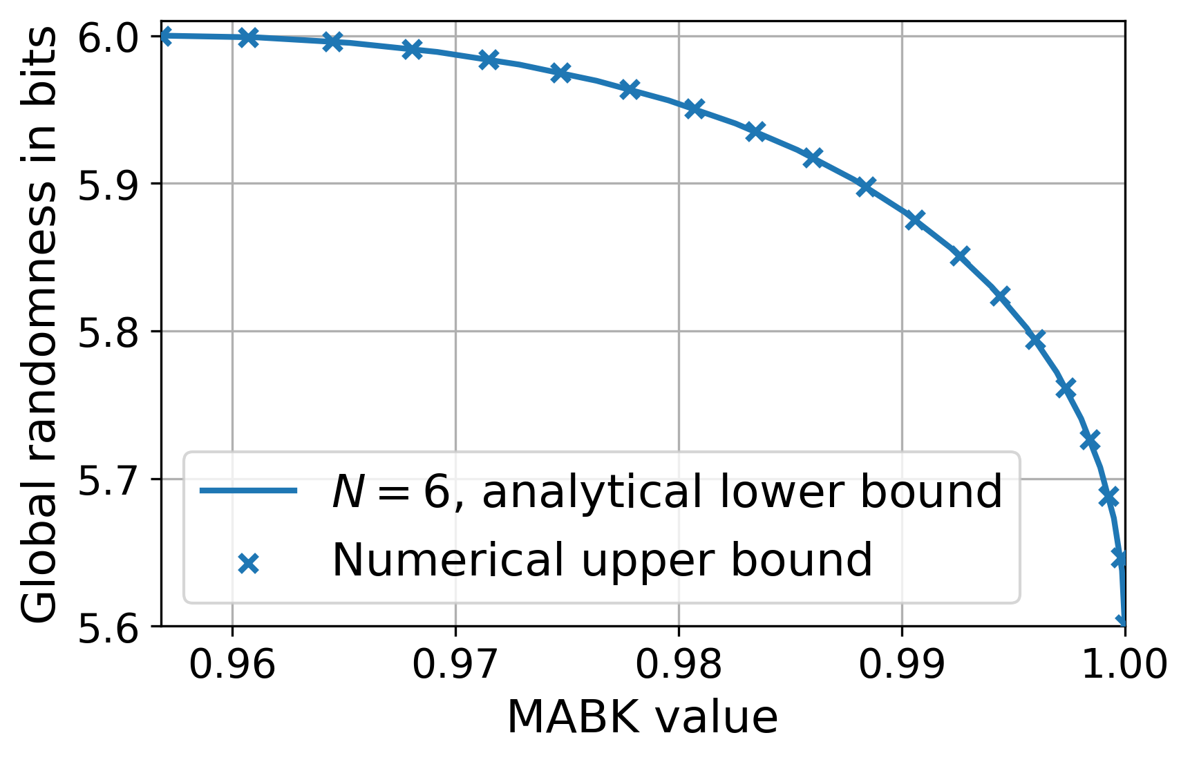
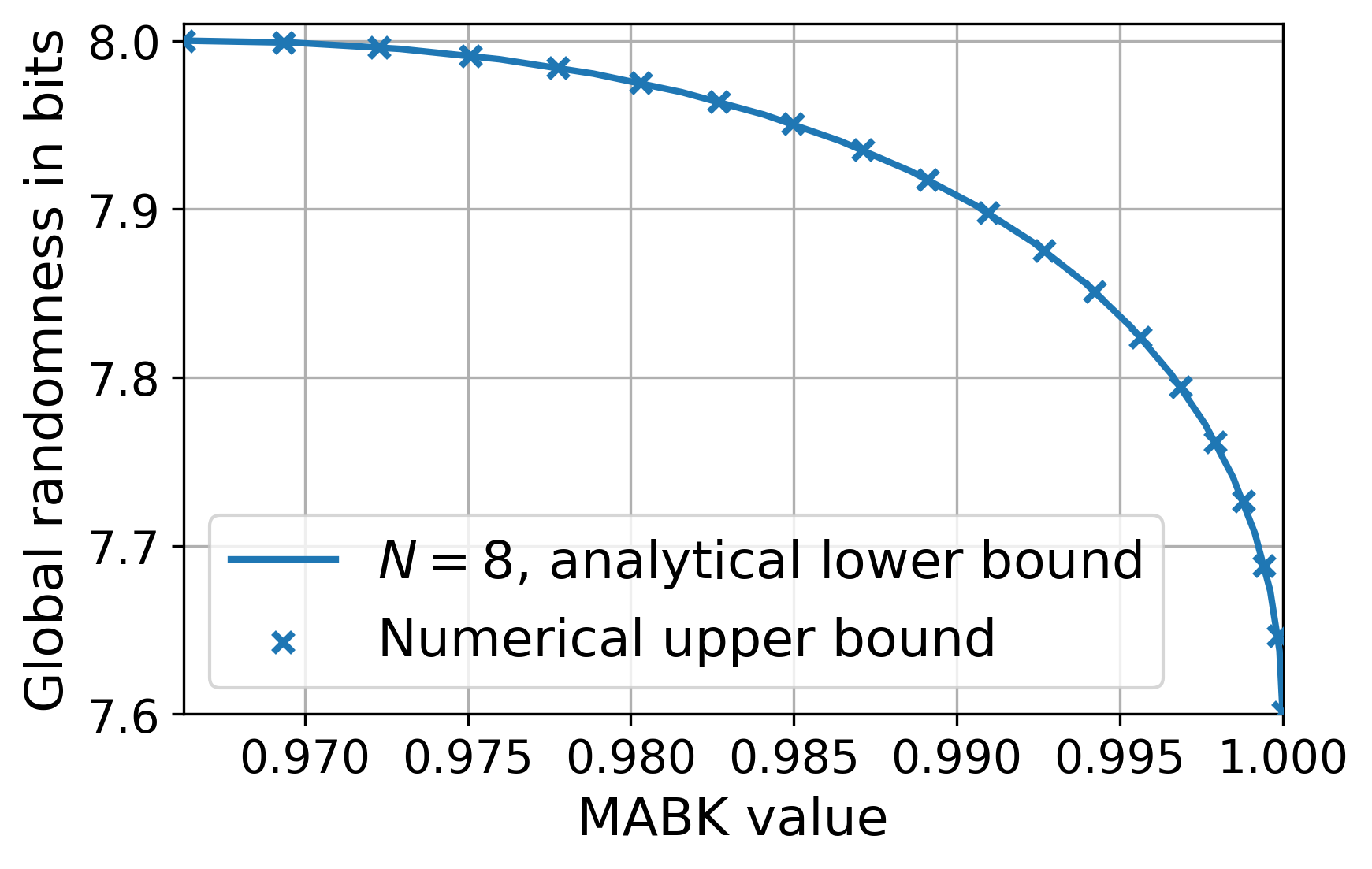
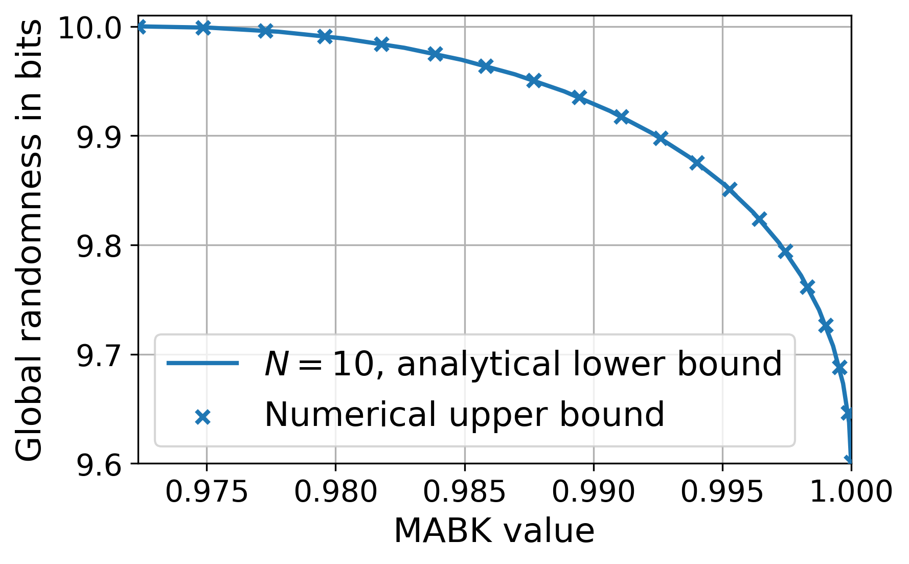
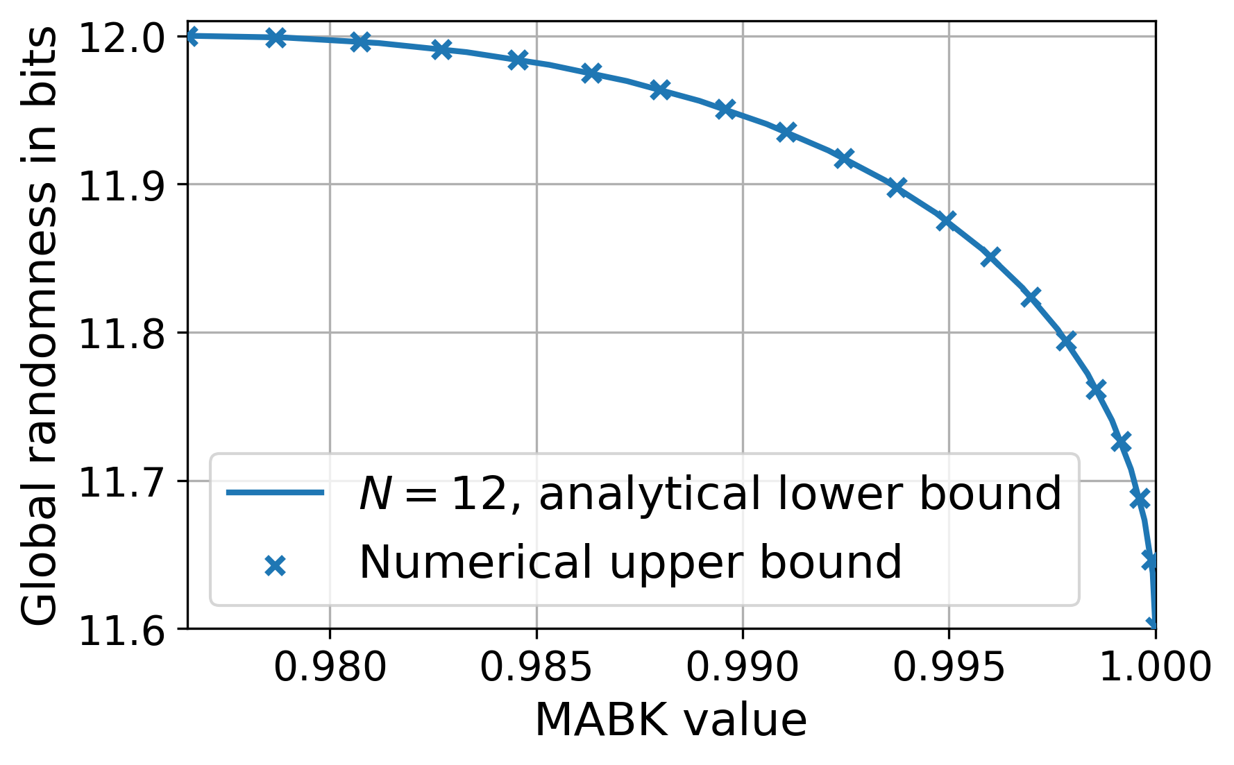
Figure 6: Lower bounds on the maximum DI randomness versus MABK value, normalized by the maximum quantum value $2^{(N-1)/2}$, for even $N$. These are compared to numerical upper bounds computed via the SOS technique. Each plot starts at the conjectured maximum MABK value achievable with maximum randomness, $m_{N}^{*}$, and ends with the maximum quantum MABK value. The two curves coincide well, supporting our conjecture that the analytical lower bound provided in the text is tight.

Facet	$\eta^{\mathrm{L}}$	$s^{*}$	$\eta^{\mathrm{Q}}$	$r(\langle S_{3}\rangle=\eta^{\mathrm{Q}})$
$M_{3}$	1	2	2	3
$S_{1}$	1	1.64621108	$5/3\approx 1.66666667$	$2+H_{\mathrm{bin}}(2/3)\approx 2.91829583$
$S_{2}$	2	2.59807617	$2\sqrt{2}\approx 2.82842712$	$7/2-\log_{2}(1+\sqrt{2})/\sqrt{2}\approx 2.60087604$
$S_{3}$	2	$3\sqrt{3}/2\approx 2.59807621$	$2\sqrt{2}\approx 2.82842712$	$5/2-\log_{2}(1+\sqrt{2})/\sqrt{2}\approx 1.60087604$
$S_{4}$	1	0	1	0

Table 2: Relevant bounds on violations of all inequivalent facet classes of the local polytope in the $N=3$ scenario, with two measurement per party, given in Eq. 179. $M_{3}$ is the MABK expression, $S_{1},S_{2}$ are the other non trivial facets for this scenario, $S_{3}$ is the trivial extension of CHSH and $S_{4}$ is a positivity facet . $\eta^{\mathrm{}L}$ and $\eta^{\mathrm{Q}}$ are the local and quantum bounds respectively, and $s^{*}$ is the computed upper bound on the maximum value achievable with maximum randomness. $r(\langle S_{3}\rangle=\eta^{\mathrm{Q}})$ is an upper bound on the asymptotic global DI randomness when the maximum quantum violation is achieved. The cases $M_{3}$ and $S_{3}$ are known to be tight Dhara et al. (2013); Wooltorton et al. (2022). Due to its structure, $S_{2}$ retains the same characteristics as CHSH Wooltorton et al. (2022), whereas $S_{1}$ exhibits an unexplored trade-off.

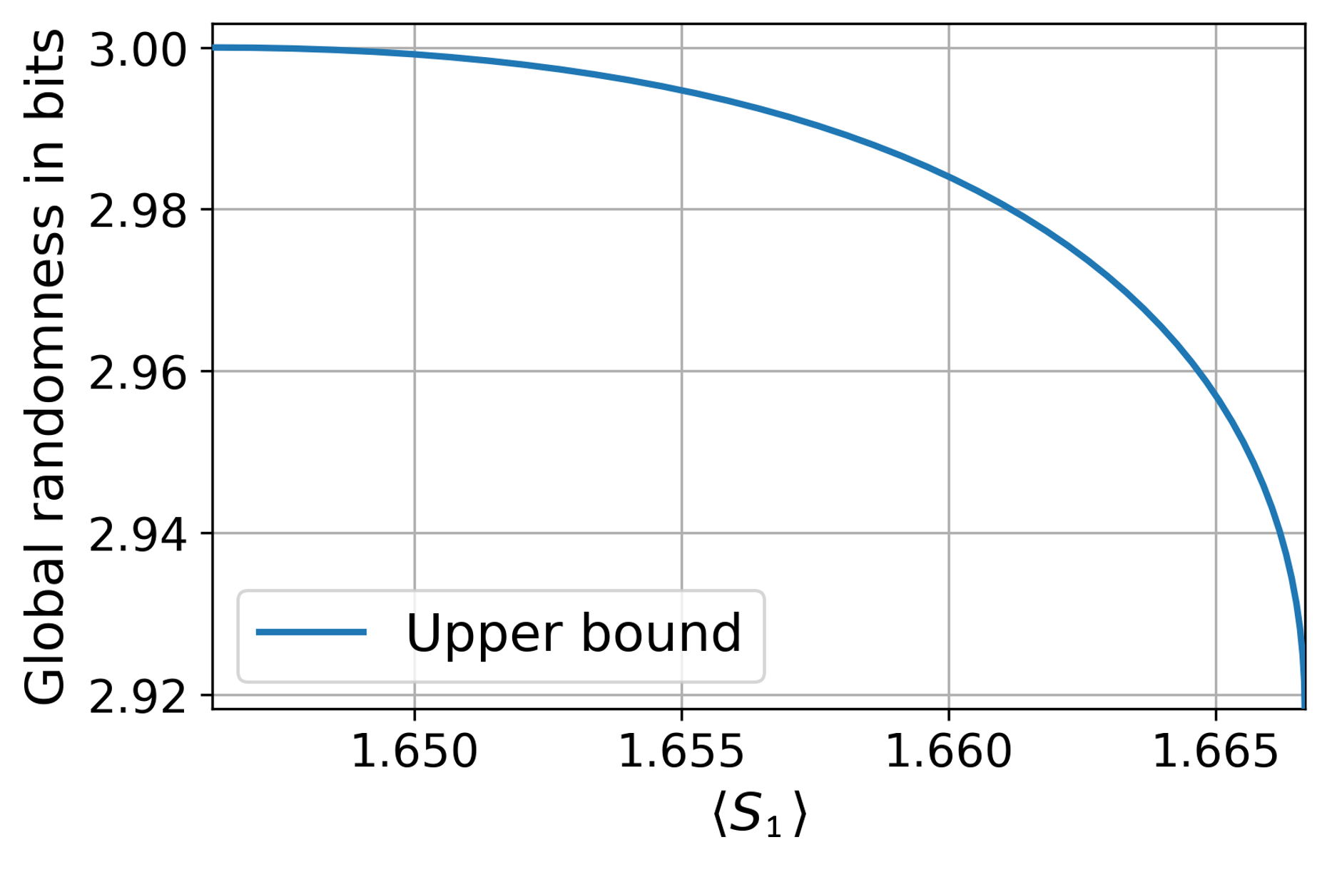
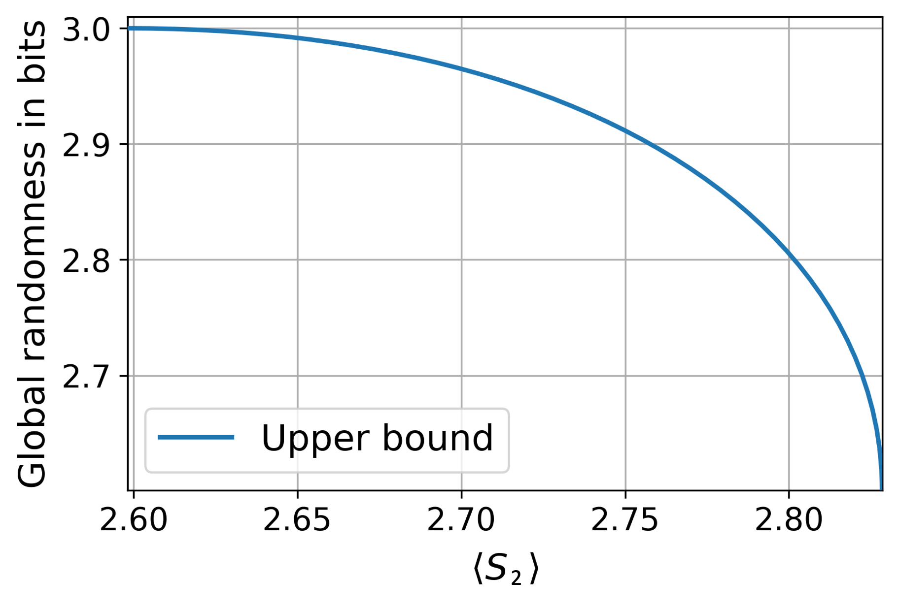
Figure 7: Upper bounds on the trade-off between global DI randomness generation and violation of non-trivial facets in the tripartite scenario with two binary measurements per party. The bounds are numerical and generated by our SOS technique. $S_{1}$ and $S_{2}$ are two non-trivial extremal Bell expressions given in Eq. 179. Details of the exact numerical values are given in Table 2.