h KA-TP-18-2023
Dark Coloured Scalars Impact on Single and Di-Higgs Production at the LHC

Abstract

The search for Dark Matter (DM) at colliders is primarily pursued via the detection of missing energy in particular final states. These searches are based on the production and decay processes where final states include DM particles and at least one Standard Model (SM) particle. DM will then reveal itself as missing energy. An alternative form to get a hint of a dark sector is via loop contribution to SM processes. In this case, it is not even relevant if the new particles have their origin in the dark sector of the model. In this work we discuss the impact of an arbitrary number of coloured scalars in single Higgs and double Higgs production at the Large Hadron Collider (LHC), and we show their complementarity. We determine the range of variation of the corrections relative to the SM for an arbitrary number of coloured scalars $n$, and discuss in more detail the cases $n=1$ and $n=2$.

1 Introduction

Any extension of the Standard Model (SM) aiming at solving the Dark Matter (DM) puzzle has to include at least one DM candidate. One of the simplest ways to address this problem is to enlarge the scalar sector of the SM by including a dark sector, usually using a discrete symmetry, and a portal coupling that connects the two sectors. Once a minimal model that provides a DM candidate is built, one needs to make sure that it is in agreement with the current measurement of the relic density and with all results from direct and indirect detection together with the constraints imposed by collider experiments. Models with a dark sector can then be further extended to explain other unsolved issues of the SM. Ultimately, any complete extension of the SM has to be in agreement with all available experimental data.

In recent years many models have been proposed to solve other discrepancies between the SM predictions and the experimental results. A particular class of models manages to solve two of these problems simultaneously: the B-physics anomalies, related essentially to the $b\to s\mu^{+}\mu^{-}$ transition [1, 2] and the muon $g-2$ anomaly [3, 4, 5, 6, 7] while providing a sound DM candidate. However, a very recent reinterpretation of the LHCb collaborations completely washed out the discrepancy with the SM prediction in the $b\to s\mu^{+}\mu^{-}$ transition [8, 9]. Still, this type of models can be made compatible with these new results for $b\to s\mu^{+}\mu^{-}$ (compatible with the SM predictions) while still solving the DM and $g-2$ problems.

The existence of this type of models prompted us to study the contribution of the new coloured scalars, that live in the dark sector, to single and di-Higgs production. The models were discussed in great detail in [10, 11] and are based on a previous model proposed in [12]. They introduce massive coloured scalar fields which, depending on the charge assignments and $SU(2)$ quantum numbers, can lead to one or several coloured scalars. A discrete $Z_{2}$ symmetry is imposed such that the new fields from the dark sector are odd under $Z_{2}$ while the SM fields are even under this symmetry. In Ref. [10], three new fields were added to the SM, one $SU(3)_{c}$ coloured scalar, $\Phi_{3}$, one colourless scalar, $\Phi_{2}$, and one vectorlike fermion, $\chi$, with an integer electric charge of 0 or $\pm 1$. The scalars are $SU(2)_{L}$ singlets and the fermions form an $SU(2)_{L}$ doublet. This model was dubbed Model 5. In Ref. [11] a different scenario was studied with the scalars as $SU(2)_{L}$ doublets and the fermion as an $SU(2)_{L}$ singlet, and called Model 3.

As the dark sector communicates with the SM via the Higgs potential, the new scalars couple to the Higgs boson. In fact, only two types of interactions are relevant to our discussion: the Higgs couplings to the new coloured scalars and the strong couplings of the coloured scalars with the gluons with origin in the covariant derivative. Therefore the one-loop single Higgs and di-Higgs production only depend on very specific terms in the Higgs potential, the ones that connect the coloured scalars with the SM Higgs doublet. Besides that, the SM Higgs coupling to the fermions (and also the Higgs self-couplings) remain exactly the SM ones - there is no mixing of the Higgs with the other scalars as they have different quantum numbers. The coloured scalars contribute to the gluon fusion single Higgs and di-Higgs production with only one coloured scalar of electric charge $2/3$, $\phi_{q}^{+2/3}$, in Model 5, while for Model 3 there are two coloured scalars contributing with electric charges $2/3$ and $5/3$, $\phi_{q}^{+2/3}$ and $\phi_{q}^{+5/3}$, respectively. We also generalise our results to the case of an arbitrary number of coloured scalars. Note that single Higgs production is a clean probe of the Higgs portal coupling in a scenario where the extension of the SM only includes an arbitrary number of coloured scalars. The di-Higgs cross section can then be used to further confirm the structure suggested by single Higgs production. From now on we will drop the old nomenclature and just refer to the model by the number of coloured scalars.

The LHC has performed numerous searches for DM. The only truly model-independent bound in the case of coloured scalar production and decay (depending only on the mass of the coloured scalar) would be a monojet event, that relies only on the strong gauge coupling. These bounds would be valid in a scenario where the couplings of the coloured scalars to the quarks and vector-like fermions are negligible or where branching ratios that lead to visible final states are too small to be detected. However, according to [12] the best bounds are obtained in the searches for DM associated with top and bottom quarks [13]. These are more restrictive than a re-interpretation of the searches for squarks at the LHC. They conclude in [12] that the mass of coloured scalars have a rough lower bound of 1 TeV. We will use this bound in our analysis.

We finalise this section by noting that the only new coupling present in the processes to be analysed is the portal coupling. Hence, in the case $n=1$ all results will depend on only two variables, the portal coupling and the coloured scalar mass. For an arbitrary $n$ we will have $n$ portal couplings and $n$ coloured scalar masses.

The paper is organised as follows. In Sec. 2 we present the single Higgs production mode, and in Sec. 3 the di-Higgs production mode is discussed. In Sec. 4 we compare the contributions of the new physics models to single Higgs and double Higgs production. Our conclusions are given in Sec. 5.

2 Single Higgs Production

We consider $n$ independent coloured complex scalars $\phi_{q}^{i=1,...,n}$ transforming in the fundamental representation of $SU(3)_{c}$. After electroweak symmetry breaking, the potential relevant to this work is given by

$$V=\sum_{i=1}^{n}\bigg{[}\underbrace{(\mu_{\phi_{q}^{i}}^{2}+\frac{v^{2}}{2}\lambda_{h\phi_{q}^{i}})}_{m_{\phi_{q}^{i}}^{2}}|\phi_{q}^{i}|^{2}+\frac{1}{2}\lambda_{h\phi_{q}^{i}}h^{2}|\phi_{q}^{i}|^{2}+v\lambda_{h\phi_{q}^{i}}h|\phi_{q}^{i}|^{2}+\lambda_{\phi_{q}^{i}}|\phi_{q}^{i}|^{4}+...\bigg{]}+...\ \ ,$$ (1)

where the couplings $\lambda_{h\phi_{q}^{i}}$ and $\lambda_{\phi_{q}^{i}}$ are real and we have defined the masses of the fields by

$$m_{\phi_{q}^{i}}^{2}=\mu_{\phi_{q}^{i}}^{2}+\frac{v^{2}}{2}\lambda_{h\phi_{q}^{i}}\ .$$ (2)

Note that there are in total $3n$ independent parameters. If we also consider that these $n$ fields form an $SU(2)_{L}$ multiplet, $\Phi_{q}=\matrixquantity*(\phi_{q}^{1}&\phi_{q}^{2}&...&\phi_{q}^{n})^{\text{{T}}}$, this would impose the following constraints: $\mu_{\phi_{q}^{i}}^{2}=\mu_{\phi_{q}^{k}}^{2}\equiv\mu_{\Phi_{q}}^{2}$ and $\lambda_{\phi_{q}^{i}}=\lambda_{\phi_{q}^{k}}\equiv\lambda_{\Phi_{q}}$. We are now left with only $n+2$ degrees of freedom. This implies that for equal portal couplings $\lambda_{h\phi_{q}^{i}}$ the masses $m_{\phi_{q}^{i}}^{2}$ given by Eq. (2) are also equal and vice-versa. For this work we will consider the more general case of $n$ independent fields but still assuming that they never have the exact same quantum numbers.

Single Higgs production via gluon fusion, which is the main production process at the LHC, proceeds at leading order (LO) in the SM via quark loops [14] as shown in Fig. 1(a), with the heavier quarks giving the major contribution. In the new models, which we will refer to as BDM models, two new diagrams emerge as shown in Figs. 1(b) and 1(c) .

(a)

(b)

(c)

Figure 1: Generic single Higgs production diagrams. (a) - SM quark loops; (b)/(c) - BDM coloured scalars loops.

The amplitude for this process can be cast into the form

$$\mathcal{M}_{\triangle}^{gg\rightarrow h}=\frac{g_{s}^{2}m_{h}^{2}}{16\pi^{2}}\bigg{(}\sum_{Q}g_{Q}^{h}F_{\triangle}^{Q}+\sum_{\phi_{q}^{i}}g_{\phi_{q}^{i}}^{h}F_{\triangle}^{\phi_{q}^{i}}\bigg{)}\ A_{1\mu\nu}\ \epsilon_{a}^{\mu}\epsilon_{b}^{\nu}\ \delta_{ab},$$ (3)

where the indices $a$ and $b$ are associated with the incoming gluons, $A_{1}^{\mu\nu}=g^{\mu\nu}-p_{b}^{\mu}p_{a}^{\nu}/p_{a}\cdot p_{b}$ and the quark and scalar form factors are given by [15]

$$F_{\triangle}^{Q} =\tau_{Q}\left(1+(1-\tau_{Q})f(\tau_{Q})\right),\qquad g_{Q}^{h} =\frac{1}{v},$$ (4)

$$F_{\triangle}^{\phi_{q}^{i}} =-\frac{1}{2}\tau_{\phi_{q}^{i}}\left(1-\tau_{\phi_{q}^{i}}f(\tau_{\phi_{q}^{i}})\right),\qquad g_{\phi_{q}^{i}}^{h} =\frac{\lambda_{h\phi_{q}^{i}}v}{2m_{\phi_{q}^{i}}^{2}},$$ (5)

with $\tau_{X}=4m_{X}^{2}/m_{h}^{2}$ ($X=Q,\phi_{q}^{i}$) and $f(\tau)$ defined as

$$f(\tau)=\left\{\begin{array}[]{ll}\arcsin(\frac{1}{\sqrt{\tau}})^{2}&\tau\geq 1\\ -\frac{1}{4}\left[\log(\frac{1+\sqrt{1-\tau}}{1-\sqrt{1-\tau}})-i\pi\right]^{2}&\tau<1\end{array}\right.\ \ .$$ (6)

In the limit of large masses the form factors approach a constant value,

$$\lim_{m_{Q}^{2}\rightarrow\infty}F_{\triangle}^{Q} = \frac{2}{3}\ ,$$ (7)

$$\lim_{m_{\phi_{q}^{i}}^{2}\rightarrow\infty}F_{\triangle}^{\phi_{q}^{i}} = \frac{1}{6}\ ,$$ (8)

and therefore the large mass behaviour is determined solely by the coupling pre-factors $g_{X}^{h}$. Consequently, for large masses, the scalar loop contribution to the amplitude is suppressed by a factor of $1/m_{\phi_{q}^{i}}^{2}$. Because the quark Yukawa couplings are proportional to their masses, the quark loop contribution approaches a constant value for large masses. Thus, although this process can be used to determine how many heavy quarks are present in the model the same is not true for the coloured scalars. In Fig. 2 we present $f(\tau)$ as a function of $\tau$ in the left plot and the quark and scalar form factors as a function of $\tau$ in the right plot, which nicely shows that the two form factors approach constant values in the large mass limit.

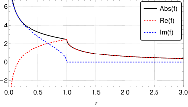
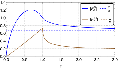
Figure 2: Left: $f(\tau)$ as a function of $\tau$; right: quark and scalar form factors as a function of $\tau$.

2.1 The LHC Production Cross Section

The calculation of the gluon fusion production cross section is performed at LO by implementing the new form factors for the coloured scalars (Eq. (5)) in the program HIGLU [16] which can be used to calculate the single Higgs production cross section at the LHC in the SM and in the Minimal Supersymmetric extension of the SM (MSSM). In the SM the $gg$ initiated production is much larger than its quark counterpart making the latter negligible in SM-like models, such as the ones discussed in this work. We can therefore write the hadronic cross section as

$$\sigma(pp\rightarrow h)=\sigma_{0}^{h}\tau_{h}\derivative{\mathcal{L}^{gg}}{\tau_{h}},\qquad\qquad\sigma_{0}^{h}=\frac{\pi}{16m_{h}^{4}}\left|\mathcal{M}_{\triangle}^{gg\rightarrow h}\right|^{2},$$ (9)

where $\derivative{\mathcal{L}^{gg}}{\tau_{h}}$ is the gluon luminosity and $\tau_{h}=m_{h}^{2}/s$, with $s$ denoting the total hadronic c.m. energy squared. In order to reduce the impact of the important higher-order (HO) effects we calculate the relative deviation of the new physics (NP) cross section in our model from the SM cross section, defined as

$$\delta_{h}=\frac{\sigma_{NP}-\sigma_{SM}}{\sigma_{SM}}.$$ (10)

We hence assume that the relative HO corrections to the new physics cross section in our model do not deviate significantly from those of the SM case which can safely be assumed for the QCD corrections while for the EW corrections this is not necessarily the case. The latter are, however, small compared to the QCD corrections. Using Eqs. (3–5) and Eq. (9), we can write $\delta_{h}$ as

$$\delta_{h}=\frac{\left|\sum_{Q}F_{\triangle}^{Q}+v\sum_{\phi_{q}^{i}}g_{\phi_{q}^{i}}^{h}F_{\triangle}^{\phi_{q}^{i}}\right|^{2}-\left|\sum_{Q}F_{\triangle}^{Q}\right|^{2}}{\left|\sum_{Q}F_{\triangle}^{Q}\right|^{2}}=2v\sum_{\phi_{q}^{i}}g_{\phi_{q}^{i}}^{h}\operatorname{Re}\left[\frac{F_{\triangle}^{\phi_{q}^{i}}}{\sum_{Q}F_{\triangle}^{Q}}\right]+v^{2}\frac{\left|\sum_{\phi_{q}^{i}}g_{\phi_{q}^{i}}^{h}F_{\triangle}^{\phi_{q}^{i}}\right|^{2}}{\left|\sum_{Q}F_{\triangle}^{Q}\right|^{2}}.$$ (11)

For the following numerical analysis we include the bottom, charm and top quark loops in single Higgs production, while in double Higgs production only top and bottom quark loops are taken into account. We use the following input values for the Higgs, top, bottom and charm quark masses, respectively:

$$m_{h}=125\mbox{ GeV},\quad m_{t}=172.5\mbox{ GeV},\quad m_{b}=4.75\mbox{ GeV},\quad m_{c}=1.43\mbox{ GeV}.$$ (12)

We use the LO pdfs NNPDF40_lo_as_01180 [54, 55] and the LO strong coupling constant

$$\alpha_{s}=0.118\;.$$ (13)

The cross sections are calculated for a c.m. energy of $\sqrt{s}=14$ TeV. Note that the dependence on $\sqrt{s}$ cancels out in $\delta_{h}$.

2.2 Model with One Scalar versus a Model with Two Scalars

Let us start by considering the scenarios $n=1$ (just one coloured scalar) and $n=2$ (two coloured scalars). As already discussed, all scalar masses will be taken to be above 1 TeV. In the case $n=1$ and considering here, for the sake of the discussion, only the top quark contribution (the bottom contribution only ranges at the percent level), the following simplified form for $\delta_{h}$ is obtained

$$\delta_{h}=\lambda_{h\phi_{q}^{1}}\frac{v^{2}}{m_{\phi_{q}^{1}}^{2}}\left(\frac{F_{\triangle}^{\phi_{q}^{1}}}{F_{\triangle}^{Q}}\right)+\lambda_{h\phi_{q}^{1}}^{2}\frac{v^{4}}{4m_{\phi_{q}^{1}}^{4}}\left(\frac{F_{\triangle}^{\phi_{q}^{1}}}{F_{\triangle}^{Q}}\right)^{2}.$$ (14)

Any extension with more than one coloured scalar will have one more effective Higgs-scalar coupling $\lambda_{h\phi_{q}^{i}}$ and one more scalar mass $m_{\phi_{q}^{i}}$ for each new scalar added to the model. Thus, in order to simplify the presentation of the results, we impose the constraint of equal coloured scalar masses for any extension with more than one coloured scalar. As we will show later, for masses above 5 TeV the cross sections will be very small unless the number of scalars becomes very large. So the interesting range for the mass is indeed very small. Note that in the plots presented later we will always include the bottom, charm and top contributions.

In the BDM models, the quartic coupling $\lambda_{h\phi_{q}^{i}}$ that enters the calculation of the cross section is an effective coupling in the following sense: in the case $n=1$ it is just the portal coupling between the Higgs and the singlet coloured scalar; for $n=2$, the two effective couplings are the sum of combinations of three portal couplings (in the case of an $SU(2)$ representation). In more detail, for $n=1$ the coloured scalar is an $SU(2)$ singlet and the portal coupling with the Higgs doublet can be written as

$$V_{\text{portal}}^{n=1}=\lambda_{H\Phi_{q}}|H|^{2}|\Phi_{q}|^{2}\;,$$ (15)

and the effective coupling takes the form

$$\lambda_{h\phi_{q}^{1}}=\lambda_{H\Phi_{q}}\,.$$ (16)

In the scenario $n=2$ the coloured scalar is an $SU(2)$ doublet and the portal couplings are now

$$V_{\text{portal}}^{n=2}=\lambda_{H\Phi_{q}}|H|^{2}|\Phi_{q}|^{2}+\lambda^{\prime}_{H\Phi_{q}}|H^{\dagger}\Phi_{q}|^{2}+y_{H\Phi_{q}}|H^{\dagger}i\sigma_{2}\Phi_{q}|^{2},$$ (17)

which results in two effective couplings,

$$\lambda_{h\phi_{q}^{1}}=\lambda_{H\Phi_{q}}+\lambda^{\prime}_{H\Phi_{q}}\ ,\qquad\lambda_{h\phi_{q}^{2}}=\lambda_{H\Phi_{q}}+y_{H\Phi_{q}}.$$ (18)

We have also checked that the same applies to the triplet representation of $SU(2)$ [56]. However, one should stress that what is relevant here is that we will discuss any type of model with an arbitrary number of scalars, each with an effective portal coupling and a given mass. The results can then be translated to any specific model of this kind.

Since all form factors are positive and strictly decreasing for $m_{\phi_{q}^{i}}>1$ TeV, the highest contributions to the cross sections will be achieved when these form factors are at their highest value corresponding to the lowest mass for all the scalars. Under the equal masses constraint ($m_{\phi_{q}^{i}}=m_{\phi_{q}^{j}}\equiv m_{\phi_{q}}\Rightarrow F_{\triangle}^{\phi_{q}^{i}}=F_{\triangle}^{\phi_{q}^{j}}\equiv F_{\triangle}^{\phi_{q}}$) we can write

$$\delta_{h}=\left(\sum_{i}\lambda_{h\phi_{q}^{i}}\right)\frac{v^{2}}{m_{\phi_{q}}^{2}}\left(\frac{F_{\triangle}^{\phi_{q}}}{F_{\triangle}^{Q}}\right)+\left(\sum_{i}\lambda_{h\phi_{q}^{i}}\right)^{2}\frac{v^{4}}{4m_{\phi_{q}}^{4}}\left(\frac{F_{\triangle}^{\phi_{q}}}{F_{\triangle}^{Q}}\right)^{2}.$$ (19)

With all masses equal, $\delta_{h}$ is not sensitive to individual couplings but only to their total sum, $\sum_{i}\lambda_{h\phi_{q}^{i}}$. Further, taking all couplings equal, $\lambda_{h\phi_{q}^{i}}=\lambda_{h\phi_{q}^{j}}\equiv\lambda_{h\phi_{q}}$, we still cover the full range of possible values for $\delta_{h}$ because for any particular choice of couplings $\{\lambda_{h\phi_{q}^{1}},...,\lambda_{h\phi_{q}^{n}}\}$ there is always a single coupling $\lambda_{h\phi_{q}}$ such that $\sum_{i}\lambda_{h\phi_{q}^{i}}=n\lambda_{h\phi_{q}}$ which will give equivalent results for $\delta_{h}$. With this approximation the coupling $\lambda_{h\phi_{q}}$ will just be rescaled by a factor $n$ when going from the case $n=1$ to arbitrary $n$.

Before presenting the results we will discuss the allowed values for the couplings. As the upper bound we will consider the perturbativity bound of $4\pi$. For the lower bound, one of the conditions for the potential (Eq. (1)), to be bounded from below, following the same procedure as in [57], gives rise to the following constraint

$$\lambda_{h\phi_{q}^{i}}\geq-\frac{m_{h}}{v}\sqrt{2\lambda_{\phi_{q}^{i}}}\,,$$ (20)

where $m_{h}$ is the SM Higgs boson mass and $\lambda_{\phi_{q}^{i}}$ is the $\phi_{q}^{i}$ quartic self coupling parameter that must be positive, $\lambda_{\phi_{q}^{i}}\geq 0$, and obey the perturbativity bound of $\lambda_{\phi_{q}^{i}}\leq 4\pi$. Therefore we will vary the relevant parameters $\lambda_{h\phi_{q}^{i}}$ between the lower value given by Eq. (20) and the upper value $4\pi$.

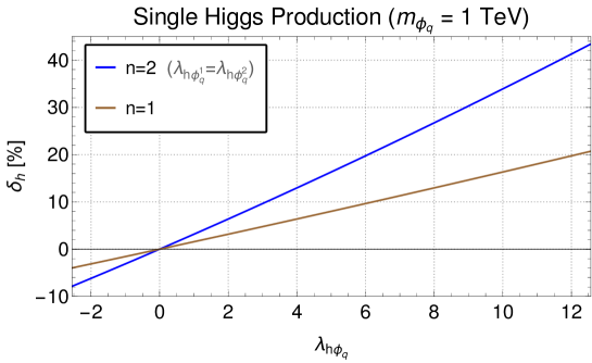
Figure 3: $\delta_{h}$ as a function of the effective portal coupling $\lambda_{h\phi_{q}}$ for a mass of $m_{\phi_{q}}=1$ TeV and for $n=1$ and $n=2$.

In Fig. 3 we present the results for $\delta_{h}$ as a function of the effective portal coupling $\lambda_{h\phi_{q}}$ for a mass of $m_{\phi_{q}}=1$ TeV and for $n=1$ and $n=2$. The single Higgs cross section was calculated with HIGLU for a c.m. energy of 14 TeV resulting in a SM LO cross section of $\sigma^{h}_{SM}=15.76$ pb for the above given input values. It is evident that $\delta_{h}$ varies linearly with the effective coupling $\lambda_{h\phi_{q}}$, which means that, in this range, the interference term between the SM and NP form factors is dominant. The large scalar masses we are working with and the fact that the interference term is proportional to only $1/m_{\phi_{q}}^{2}$ while the purely NP contributions are suppressed by a factor of $1/m_{\phi_{q}}^{4}$ (cf. Eq. (14)), are the reason behind this behaviour.

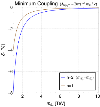
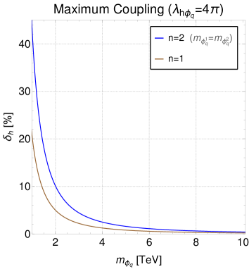
Figure 4: $\delta_{h}$ as a function of the coloured scalar mass for the minimum value of the coupling (left) and the maximum value of the coupling (right) and for $n=1$ and $n=2$.

In Fig. 4 we show the results for $\delta_{h}$ as a function of the coloured scalar mass for the minimum value of the coupling (left) and the maximum value of the coupling (right) and for $n=1$ and $n=2$. Since, as argued above, the interference term is dominant, $\delta_{h}$ behaves approximately as $1/m_{\phi_{q}}^{2}$ for fixed $\lambda_{h\phi_{q}}$. For the allowed range of variation the maximum value of variation relative to the SM is between about -10% and +40%.

The NP term only becomes comparable to the interference term in the limit

$$\lambda_{h\phi_{q}}=\frac{4m_{\phi_{q}}^{2}}{v^{2}}\frac{F_{\triangle}^{Q}}{F_{\triangle}^{\phi_{q}}}\xrightarrow[m_{\phi_{q}}\to\infty]{m_{Q}\to\infty}\frac{16m_{\phi_{q}}^{2}}{v^{2}},$$ (21)

which means that for a mass of $m_{\phi_{q}}=1$ TeV $\lambda_{h\phi_{q}}\approx 260$ for $n=1$. As more scalars are added the picture can change. As the interference term scales with $n$ and the NP term scales as $n^{2}$, for a number of scalars above 20 and all masses equal to 1 TeV the NP term starts to dominate.

2.3 Models with $n$ Coloured Scalars

In the previous section we have set all masses to be equal. Relaxing this condition forces us to return to the more general expression given in Eq. (11). However, we can follow a different approach in order to simplify the final expression by taking advantage of the large scalar masses and using the limit for $F_{\triangle}^{\phi_{q}^{i}}$ given in Eq. (8). For scalar masses above 1 TeV the error in $F_{\triangle}^{\phi_{q}^{i}}$ by using this limit is only about 0.2%. With this approximation $\delta_{h}$ can be written as

$$\delta_{h}=\frac{1}{\left|\sum_{Q}F_{\triangle}^{Q}\right|}\frac{v^{2}}{6}\sum_{i}\frac{\lambda_{h\phi_{q}^{i}}}{m_{\phi_{q}^{i}}^{2}}+\frac{1}{\left|\sum_{Q}F_{\triangle}^{Q}\right|^{2}}\frac{v^{4}}{144}\left(\sum_{i}\frac{\lambda_{h\phi_{q}^{i}}}{m_{\phi_{q}^{i}}^{2}}\right)^{2},$$ (22)

where we have $\left|\sum_{Q}F_{\triangle}^{Q}\right|\approx 0.641$ when including the top, bottom and charm quarks. Including only the top quark and the limit in Eq. (7) would imply an error in $\left|\sum_{Q}F_{\triangle}^{Q}\right|$ of around  4%. This approximation has the advantage of allowing us to write the results as a function of the ratio $x_{i}=\lambda_{h\phi_{q}^{i}}/m_{\phi_{q}^{i}}^{2}$ where the index $i$ represents each scalar. It is now clear that we can show $\delta_{h}$ as a function of the sum $(\sum_{i}x_{i})$. As previously discussed, as long as we span all possible values for this sum we will also have fully explored all values that $\delta_{h}$ can take. In order to do this let us first note that the minimum and maximum of $(\sum_{i}x_{i})$ are achieved when all $x_{i}$ are at their minimum and maximum values, respectively. Hence, to generate all values for the sum and consequently for $\delta_{h}$, we can make the simple choice of $x_{i}=x_{j}$ with the limits of $\min(x_{i})=\min\left(\lambda_{h\phi_{q}^{i}}/m_{\phi_{q}^{i}}^{2}\right)=-(8\pi)^{1/2}m_{h}/v\,\text{TeV}^{-2}$ and $\max(x_{i})=\max\left(\lambda_{h\phi_{q}^{i}}/m_{\phi_{q}^{i}}^{2}\right)=4\pi\ \text{TeV}^{-2}$ where we have considered $\min(m_{\phi_{q}^{i}})=1\ \text{TeV}$.

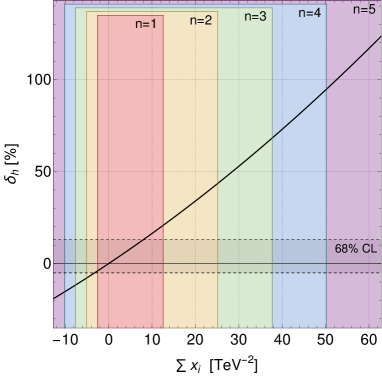
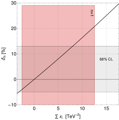
Figure 5: $\delta_{h}$ as a function of $\sum_{i}x_{i}$. The minimum and maximum limits for a model with $n$ scalars are indicated by the coloured zones, where a minimum mass of $m_{\phi_{q}^{i}}=1$ TeV is considered and the couplings are varied between the lower bound of $-(8\pi)^{1/2}m_{h}/v$ and the perturbativity upper bound of $4\pi$. In the left plot the horizontal lines are taken from the ATLAS combination [58] and show the $1\sigma$ results for Higgs production via gluon fusion. In the right plot we present just the case $n=1$ for a better understanding of the bounds on $\sum_{i}x_{i}$ for $n=1$.

In Fig. 5 we show $\delta_{h}$ as a function of $\sum_{i}x_{i}$. The minimum and maximum limits for a model with $n$ scalars are indicated by the coloured zones, where a minimum mass of 1 TeV is considered and the couplings are varied between their minimum and maximum allowed values. The horizontal lines represent the relative experimental uncertainty of the experimental results for Higgs production via gluon fusion at $1\sigma$. In the left plot the lines are taken from the ATLAS combination [58] at 13 TeV and 80 fb^-1, leading to $\delta_{h}\in[-5,13]$. In the right plot we present just the case $n=1$ for a better understanding of the bounds on $\sum_{i}x_{i}$ for $n=1$. Considering $n=1$ we can see that $-3.2<\sum_{i}x_{i}<8$ approximately. This in turn means that for a mass of 1 TeV the coupling is also constrained to be $-3.2<\lambda_{h\phi_{q}^{1}}<8$. Therefore the bounds are not very strong at the moment but are already better than the perturbative limit for the upper bound. Still, as the mass grows the bound on the coupling gets weaker. For $n>1$ if the couplings are all of the same order, the constraints will be stronger if again the masses are all of the order 1 TeV. But there is always the possibility of having all couplings very small except one, recovering the $n=1$ constraints for the larger coupling. Furthermore, if the couplings have different signs we end up with a larger freedom than for the case $n=1$. These scenarios will have to be studied for the specific model in question using every other information on the model.

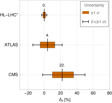
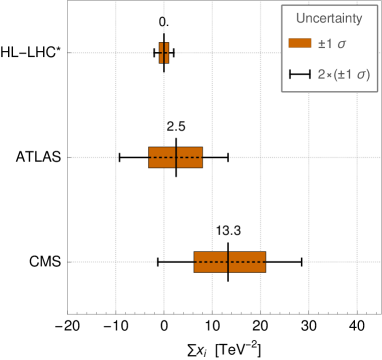
Figure 6: Allowed values of $\delta_{h}$ (left) and $\sum_{i}x_{i}$ (right) at $1\sigma$ and $2\times 1\sigma$ using the present experimental limits from ATLAS [58], CMS [59], and the predictions for the future HL-LHC [60].

In Fig. 6 we show the allowed values of $\sum_{i}x_{i}$ (left) and $\delta_{h}$ (right) at $1\sigma$ and $2\times 1\sigma$ using the present experimental limits from ATLAS [58], CMS [59], and the predictions for the future HL-LHC [60]. The predictions for the HL-LHC show that we will attain a result of the order $\delta_{h}\in[-1.6,1.6]$.

3 Double Higgs Production

Similar to the single Higgs case, the production of a pair of Higgs bosons is dominated by the gluon fusion process, which at LO is given by a triangle and a box diagram with heavy quarks running in the loop [61]. The new coloured scalars will contribute to di-Higgs production by similar loop diagrams. Due to the new 2 gluon-2 coloured scalars and 2 Higgs-2 coloured scalars couplings, however, there are now additional topologies that contribute to the process.

3.1 The Leading-Order Amplitude

The complete set of diagrams is given by the ones involving the trilinear Higgs self-coupling, shown in Fig. 7, and diagrams that do not depend on it, depicted in Fig. 8. The new topologies arising in our model are given in Fig. 7 (b) and (c) and in Fig. 8 (b)-(e). As in the SM, we have triangle and box topologies and now additionally also a self-energy-like topology.

(a)

(b)

(c)

Figure 7: Generic diagrams contributing to double Higgs production involving the trilinear Higgs self-coupling: (a) - SM quark loop; (b)/(c) - coloured scalars loop.

(a)

(b)

(c)

(d)

(e)

Figure 8: Generic diagrams contributing to double Higgs production independent of the trilinear Higgs self-coupling. (a) - SM quark loop; (b-e) - coloured scalars loop.

The LO amplitude can be decomposed into two different tensor structures, which correspond to total gluon spin 0 and 2, respectively, along the collision axis. They are given by [62]

$$A_{1}^{\mu\nu} =g^{\mu\nu}-\frac{p_{b}^{\mu}p_{a}^{\nu}}{\left(p_{a}p_{b}\right)}$$ (23)

$$A_{2}^{\mu\nu} =g^{\mu\nu}+\frac{1}{p_{T}^{2}(p_{a}p_{b})}\left[\left(p_{c}^{2}\right)p_{b}^{\mu}p_{a}^{\nu}-2\left(p_{b}p_{c}\right)p_{c}^{\mu}p_{a}^{\nu}-2\left(p_{a}p_{c}\right)p_{b}^{\mu}p_{c}^{\nu}+2\left(p_{a}p_{b}\right)p_{c}^{\mu}p_{c}^{\nu}\right]$$ (24)

with

$$A_{1}\cdot A_{1}=A_{2}\cdot A_{2}=2\,,\quad A_{1}\cdot A_{2}=0$$ (25)

and

$$p_{T}^{2}=2\frac{\left(p_{a}p_{c}\right)\left(p_{b}p_{c}\right)}{\left(p_{a}p_{b}\right)}-p_{c}^{2},$$ (26)

where $p_{a,b}$ denote the four-momenta of the two incoming gluons, and $p_{c,d}$ those of the outgoing Higgs bosons. The LO amplitude given by the diagrams in Fig. 7, which contain the trilinear Higgs self-coupling, can be cast in the form

$$\mathcal{M}_{hhh}^{gg\rightarrow hh}=\frac{g_{s}^{2}s}{16\pi^{2}}\ C_{\triangle}\left(\sum_{Q}g_{Q}^{h}F_{\triangle}^{Q}+\sum_{\phi_{q}^{i}}g_{\phi_{q}^{i}}^{h}F_{\triangle}^{\phi_{q}^{i}}\right)A_{1\mu\nu}\epsilon_{a}^{\mu}\epsilon_{b}^{\nu}\ \delta_{ab}\ ,$$ (27)

where

$$C_{\triangle}=\frac{3m_{h}^{2}/v}{s-m_{h}^{2}}\ ,$$ (28)

$\epsilon_{a,b}^{\mu/\nu}$ represent the gluon polarisation vectors and $g_{s}$ denotes the strong coupling constant. The first term in Eq. (27) corresponds to the first diagram and the second one to the last two diagrams. The form factors $F_{\triangle}^{Q/\phi_{q}^{i}}$ and the couplings $g_{Q/\phi_{q}^{i}}^{h}$ are given in Eqs (4) and (5). The amplitude independent of the Higgs self-coupling can be written as

$$\mathcal{M}_{\text{no }hhh}^{gg\rightarrow hh}=\frac{g_{s}^{2}s}{16\pi^{2}}\ C_{\square}\Bigg{[} \sum_{Q}\left((g_{Q}^{h})^{2}F_{\square}^{Q}A_{1\mu\nu}+(g_{Q}^{h})^{2}G_{\square}^{Q}A_{2\mu\nu}\right)$$

$$+ \sum_{\phi_{q}^{i}}\left(\left((g_{\phi_{q}^{i}}^{h})^{2}F_{\square_{1}}^{\phi_{q}^{i}}+g_{\phi_{q}^{i}}^{hh}F_{\square_{2}}^{\phi_{q}^{i}}\right)A_{1\mu\nu}+(g_{\phi_{q}^{i}}^{h})^{2}G_{\square_{1}}^{\phi_{q}^{i}}A_{2\mu\nu}\right)\Bigg{]}\epsilon_{a}^{\mu}\epsilon_{b}^{\nu}\ \delta_{ab}\ ,$$ (29)

where $C_{\square}=1$, the prefactors $g_{Q/\phi_{q}^{i}}^{h}$ are given in Eqs. (4) and (5) and

$$g_{\phi_{q}^{i}}^{hh}=\frac{\lambda_{h\phi_{q}^{i}}}{2m_{\phi_{q}^{i}}^{2}}\;.$$ (30)

The quark form factors $F_{\square}^{Q}$ and $G_{\square}^{Q}$ corresponding to Fig. 8 (a), which have been calculated in the literature before (cf. e.g. [62]), are deferred to the Appendix B, while the new form factors are given here. The form factor $F_{\square_{1}}^{\phi_{q}^{i}}$ sums the contributions of the diagrams Figs. 8 (b) and (c) proportional to $A_{1}^{\mu\nu}$, $F_{\square_{2}}^{\phi_{q}^{i}}$ stems from the sum of the contributions of Figs. 8 (d) and (e), and $G_{\square_{1}}^{\phi_{q}^{i}}$ is the sum of the contributions of Figs. 8 (b) and (c) proportional to $A_{2}^{\mu\nu}$. They read explicitly

$$G_{\square_{1}}^{\phi_{q}}=\frac{4m_{\phi_{q}}^{4}}{s}\left(\frac{1}{tu-m_{h}^{4}}\right)\Bigg{(}s(t+u)C_{ab}^{m_{\phi_{q}}^{2}}+(2t)(t-m_{h}^{2})C_{ac}^{m_{\phi_{q}}^{2}}+(2u)(u-m_{h}^{2})C_{bc}^{m_{\phi_{q}}^{2}}\\ -(t^{2}+u^{2}-2m_{h}^{4})C_{cd}^{m_{\phi_{q}}^{2}}-(st^{2}+2m_{\phi_{q}}^{2}(tu-m_{h}^{4}))D_{bac}^{m_{\phi_{q}}^{2}}\\ -(su^{2}+2m_{\phi_{q}}^{2}(tu-m_{h}^{4}))D_{abc}^{m_{\phi_{q}}^{2}}-(2m_{\phi_{q}}^{2}(tu-m_{h}^{4}))D_{acb}^{m_{\phi_{q}}^{2}}\Bigg{)}$$ (31)

$$F_{\square_{1}}^{\phi_{q}}=\frac{4m_{\phi_{q}}^{4}}{s}\Bigg{(}\frac{2}{s}(t-m_{h}^{2})C_{ac}^{m_{\phi_{q}}^{2}}+\frac{2}{s}(u-m_{h}^{2})C_{bc}^{m_{\phi_{q}}^{2}}\\ -(2m_{\phi_{q}}^{2})(D_{abc}^{m_{\phi_{q}}^{2}}+D_{bac}^{m_{\phi_{q}}^{2}})-(2m_{\phi_{q}}^{2}+\frac{1}{s}(tu-m_{h}^{4}))D_{acb}^{m_{\phi_{q}}^{2}}\Bigg{)}$$ (32)

where we have suppressed the i index only for convenience and

$$F_{\square_{2}}^{\phi_{q}^{i}}=F_{\triangle}^{\phi_{q}^{i}}\;,$$ (33)

with the latter given in Eq. (5). The Mandelstam variables $s,t,u$ and the scalar integrals $C_{ij}$ and $D_{ijk}$ are defined in the appendix.

3.2 The Leading-Order Cross Section

The amplitude squared for the computation of the cross section can be separated into two different parts, one for each spin projection, so that the differential partonic cross section can be cast into the form

$$\frac{d\hat{\sigma}^{hh}}{d\hat{t}}=\frac{G_{F}^{2}\alpha_{s}^{2}}{256(2\pi)^{3}}\left[\left|\mathcal{M}_{F}\right|^{2}+\left|\mathcal{M}_{G}\right|^{2}\right]\;,$$ (34)

where $G_{F}$ denotes the Fermi constant, $\alpha_{s}$ the strong coupling constant, and $\hat{t}$ the momentum transfer squared from one of the initial state gluons to one of the final state Higgs bosons. Each of the partial amplitudes $\mathcal{M}_{F/G}$ contains only the terms constructed with the $F/G$ form factors, respectively. Hence

$$\mathcal{M}_{F}\!\! = \!\!\sum_{Q}\left(C_{\triangle}\,g_{Q}^{h}F_{\triangle}^{Q}+C_{\square}\,(g_{Q}^{h})^{2}F_{\square}^{Q}\right)+\sum_{\phi_{q}^{i}}\left(C_{\triangle}\,g_{\phi_{q}^{i}}^{h}F_{\triangle}^{\phi_{q}^{i}}+C_{\square}\,\left((g_{\phi_{q}^{i}}^{h})^{2}F_{\square_{1}}^{\phi_{q}^{i}}+g_{\phi_{q}^{i}}^{hh}F_{\square_{2}}^{\phi_{q}^{i}}\right)\right)$$ (35)

$$\mathcal{M}_{G}\!\! = \!\!C_{\square}\left(\sum_{Q}g_{Q}^{h}G_{\square}^{Q}+\sum_{\phi_{Q}^{i}}(g_{\phi_{q}^{i}}^{h})^{2}G_{\square_{1}}^{\phi_{q}^{i}}\right)\ .$$ (36)

The total cross section for $hh$ production through gluon fusion at the LHC is obtained by integrating Eq. (34) over the scattering angle and the gluon luminosity,

$$\sigma(pp\rightarrow hh)=\int_{4m_{h}^{2}/s}^{1}\differential\tau_{h}\derivative{\mathcal{L}^{gg}}{\tau_{h}}\hat{\sigma}^{hh}(\hat{s}=\tau_{h}s)\,$$ (37)

where $s$ is the c.m. energy at the LHC. The numerical evaluation of the total production cross section is performed at LO with the program HPAIR [62, 67] where we have implemented the new form factors. The Fortran code HPAIR was originally written for the SM and the MSSM and calculates the double Higgs production through gluon fusion at LO and NLO in the heavy quark limit.

Also for double Higgs production we present our results as a ratio with respect to the SM value in order to minimise the contribution of HO effects, that is $\delta_{hh}$ is defined as

$$\delta_{hh}=\frac{\sigma_{NP}-\sigma_{SM}}{\sigma_{SM}}\,.$$ (38)

This assumes that the HO corrections in our model do not differ significantly from those of the SM, which is a rather good approximation for the QCD corrections, whereas not necessarily for the EW corrections, for which at present only first partial results exist, however, and which are expected to be less important. In contrast to single Higgs production we cannot find a simple analytic formula for this quantity due to the more involved form of the amplitudes and consequently also of the cross sections and the dependence of the form factors on the c.m. energy.

3.3 Phenomenological Analysis of the Cases $n=1$ and $n=2$

Let us start with the simpler scenarios with one or two coloured scalars. The dependence of the form factors on the mass is not trivial. Since the NP contributions should decouple from the SM for very large masses this means that $\delta_{hh}$ would eventually behave as a strictly decreasing function of the coloured scalar mass.

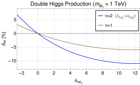
Figure 9: $\delta_{hh}=(\sigma_{NP}-\sigma_{SM})/\sigma_{SM}$ as a function of the effective portal coupling $\lambda_{h\phi_{q}}$ for a mass of $m_{\phi_{q}}=1$ TeV and for $n=1$ and $n=2$.

We will follow the same approach as for single Higgs production and choose all coloured scalar masses equal to be 1 TeV. As for the couplings, while in single Higgs production with equal masses only the total sum of the couplings was relevant, in di-Higgs production the amplitude now depends on $\lambda_{h\phi_{q}^{k}}$ and $\lambda_{h\phi_{q}^{k}}^{2}$ terms. For now we will impose the constraint of equal couplings for $n=2$. In Fig. 9 we present $\delta_{hh}$ as a function of the effective portal coupling $\lambda_{h\phi_{q}}$ for a mass of $m_{\phi_{q}}=1$ TeV and for $n=1$ and $n=2$. The double Higgs cross section was calculated with HPAIR for a c.m. energy of 14 TeV. As expected, for $\lambda_{h\phi_{q}}=0$ the NP and SM LO cross sections coincide, where the SM LO cross section calculated with HPAIR amounts to 16.37 fb.

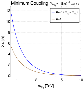
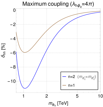
Figure 10: $\delta_{hh}=(\sigma_{NP}-\sigma_{SM})/\sigma_{SM}$ as a function of the coloured scalar mass for the minimum value of the coupling (left) and maximum value of the coupling (right) and for $n=1$ (brown) and $n=2$ (blue). The double Higgs cross section was calculated with HPAIR for a c.m. energy of 14 TeV.

In Fig. 10 we now present $\delta_{hh}$ as a function of the coloured scalar mass for the minimum (left) and maximum (value) of the effective portal coupling $\lambda_{h\phi_{q}}$ and for $n=1$ and $n=2$. As expected, the models share similar behaviours when reducing the $n=2$ case to a single coupling and mass under the equal parameters constraints which approximately double the cross section for two coloured scalars relative to the $n=1$ scenario. Since $\delta_{hh}$ depends generally on powers of $(\lambda_{h\phi_{q}})^{p}$ with $1\leq p\leq 4$, this is an indication that the linear terms seem to be the most significant ones for these results - doubling the couplings approximately doubles the cross section. Linear terms can only originate from the diagrams proportional to $\lambda_{h\phi_{q}}$ and their interference with the SM ones. This is further supported by the observation that, when $\lambda_{h\phi_{q}}>0$, the contributions to the Higgs pair production cross section are negative and, hence, odd powers of the coupling are involved. On the other hand, the shape of $\delta_{hh}$ is clearly described by a non-linear function in $\lambda_{h\phi_{q}}$. Contrary to what happened in single Higgs production, this is no longer necessarily a sign that the interference terms are insufficient to describe the results. This is due to the fact that a dependence on $\lambda_{h\phi_{q}}^{2}$ can originate from either the square of the purely NP diagrams proportional to $\lambda_{h\phi_{q}}$ (see diagrams 7(b), 7(c), 8(d), 8(e)) or from the SM interference with the NP diagrams proportional to $\lambda_{h\phi_{q}}^{2}$ (see diagrams 8(b), 8(c)). The interference term depends on $\sum_{k}(\lambda_{h\phi_{q}^{k}})^{2}$, while the term originating from squaring the NP diagrams depends on $(\sum_{k}\lambda_{h\phi_{q}^{k}})^{2}$. For $n=1$ the two dependencies are identical while for $n\geq 2$ the former represents an extra degree of freedom for $\delta_{hh}$ for a fixed $\sum_{k}\lambda_{h\phi_{q}^{k}}$. This is an important observation if we want to present the results as a function of the sum of the couplings, $\sum_{k}\lambda_{h\phi_{q}^{k}}$, as we did in the single Higgs case.

HPAIR has further been altered with the option to turn on or off particular sets of diagrams. Naturally, we will separate the ones proportional to $\lambda_{h\phi_{q}}$ and $\lambda_{h\phi_{q}}^{2}$. We further separate the two pairs of diagrams 7(b)-7(c) and 8(d)-8(e), since their form factors are the same as in single Higgs production. The sets of diagrams chosen serve the purpose of separating the contributions of the form factors $F_{\triangle}^{\phi_{q}}$, $F_{\square_{2}}^{\phi_{q}}$, which are linear in $g_{\phi_{q}}^{h}$ and $g_{\phi_{q}}^{hh}$, respectively, and $F_{\square_{1}}^{\phi_{q}}$ and $G_{\square_{1}}^{\phi_{q}}$, which are proportional to the squared coupling $(g_{\phi_{q}}^{h})^{2}$.

The results for $n=2$ are presented in Fig. 11 for a fixed mass of 1 TeV as a function of the coupling (top), for the minimum coupling as a function of the mass (middle) and for the maximum coupling as a function of the mass (bottom). The left plots show the individual contributions and the interference terms while the right plots present how the individual contributions behave with the couplings (top) and with the mass (middle and bottom). The black line represents the sum of all contributions, while the coloured lines represent the individual coloured scalar form factor contributions, separated as indicated by the legend. Note that the SM contributions drop out in $\delta_{hh}$. More specifically, the contributions denoted by the different colours are proportional to the following coloured form factors and couplings,

$$\begin{array}[]{lll}\mbox{blue}/F_{\triangle}:&\sim\{F_{\triangle}^{\phi_{q}},|F_{\triangle}^{\phi_{q}}|^{2}\}&\sim\{G_{\phi_{q}}^{h},(G_{\phi_{q}}^{h})^{2}\}\\ \mbox{red}/F_{\square_{2}}:&\sim\{F_{\square_{2}}^{\phi_{q}},|F_{\square_{2}}^{\phi_{q}}|^{2}\}&\sim\{G_{\phi_{q}}^{hh},(G_{\phi_{q}}^{hh})^{2}\}\\ \mbox{green}/F_{\square_{1}}+G_{\square_{1}}:&\sim\{F_{\square_{1}}^{\phi_{q}},G_{\square_{1}}^{\phi_{q}},|F_{\square_{1}}^{\phi_{q}}|^{2},|G_{\square_{1}}^{\phi_{q}}|^{2}\}&\sim\{G_{\phi_{q}}^{h,\,2},G_{\phi_{q}}^{h,\,2},(G_{\phi_{q}}^{h,\,2})^{2},(G_{\phi_{q}}^{h,\,2})^{2}\}\\ \mbox{violet}/F_{\triangle}\cdot F_{\square_{2}}:&\sim 2\mbox{Re}(F_{\triangle}^{\phi_{q}}F_{\square_{2}}^{\phi_{q}*})&\sim G_{\phi_{q}}^{h}\cdot G_{\phi_{q}}^{hh}\\ \mbox{orange}&\\ \quad/(F_{\triangle}+F_{\square_{2}})\cdot F_{\square_{1}}:&\sim\{2\mbox{Re}(F_{\triangle}^{\phi_{q}}F_{\square_{1}}^{\phi_{q}*}),2\mbox{Re}(F_{\square_{1}}^{\phi_{q}}F_{\square_{2}}^{\phi_{q}*})\}&\sim\{G_{\phi_{q}}^{h}\cdot G_{\phi_{q}}^{h,\,2},G_{\phi_{q}}^{h,\,2}\cdot G_{\phi_{q}}^{hh}\}\end{array}$$ (45)

where we introduced the abbreviations

$$G_{\phi_{q}}^{h}\equiv\sum_{\phi_{q}^{i}}g_{\phi_{q}^{i}}^{h}\,,\quad G_{\phi_{q}}^{hh}\equiv\sum_{\phi_{q}^{i}}g_{\phi_{q}^{i}}^{hh}\,\quad G_{\phi_{q}}^{h,\,2}\equiv\sum_{\phi_{q}^{i}}(g_{\phi_{q}^{i}}^{h})^{2}\;.$$ (46)

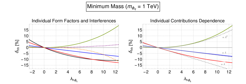
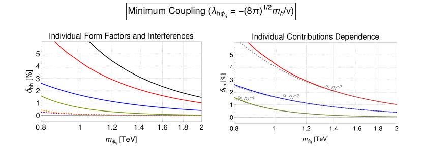
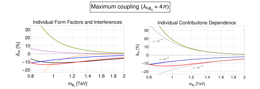
Figure 11: $\delta_{hh}$ for $n=2$ and a fixed mass of 1 TeV as a function of the coupling (top), for the minimum coupling as a function of the mass (middle) and for the maximum coupling as a function of the mass (bottom). Left: individual coloured form factor contributions and interference terms. Right: dependence of the individual contributions on the couplings (top) and the masses (middle and bottom). Black line: sum of all contributions; coloured lines: individual coloured scalar form factor contributions, separated as indicated by the legend and described in Eq. (45). The dashed lines are for the interference terms. Grey dashed lines: asymptotic behaviour in the scenario where the interference terms with the SM are the dominant ones. The grey full line at 0 in all plots is there to guide the eyes.

Note that $G_{\phi_{q}}^{hh}$ and $G_{\phi_{q}}^{h}$ only differ by a factor $1/v$. The terms linear in the form factors of the blue, red and green contribution stem from the interference with the SM form factors. The violet and orange contributions (dashed lines) hence denote the interference terms between the coloured contributions. The grey dashed lines in the right upper plot show the asymptotic behaviour in the coupling in the scenario where the interference terms with the SM are the dominant ones (where we generically denote by $\lambda$ the couplings $G_{\phi_{q}}^{h}$ (blue line) and $G_{\phi_{q}}^{hh}$ (red line) and by $\lambda^{2}$ the coupling $G_{\phi_{q}}^{h,\,2}$ (green line)). We can infer from the plot that for masses of 1 TeV and higher, both the $F_{\triangle}$ (blue line) and the $F_{\square_{1}}+G_{\square_{1}}$ (green line) contributions are rather well described by only considering their interference with the SM form factors. The $F_{\square_{2}}$ contribution (red line), however, is not well approximated by the interference with the SM contribution only. This observation is also confirmed by the middle and lower right plots which show the asymptotic behaviours in coloured masses for fixed coupling for the case that the interference term dominates.

We end this section by presenting in Fig. 12 the double Higgs corrections $\delta_{hh}$ as a function of the scalar mass $m_{\phi_{q}}$ for $n=2$. The couplings are varied between the two extreme values as discussed previously. The new physics impact due to the additional coloured loops are below 10 % already for a mass of 1 TeV and fall steeply with rising mass. Therefore the effect of two extra coloured scalar only will be extremely hard to probe even at the HL-LHC.

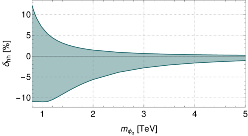
Figure 12: $\delta_{hh}$ as a function of the scalar mass $m_{\phi_{q}}$ for $n=2$. The couplings are varied between the two extreme values as discussed previously.

3.4 Model $n=2$ for Different Masses

We very briefly look at the implications of relaxing the condition of equal masses. For this, we calculated the full range of $\delta_{hh}$ for ratios between the two masses of

$$m_{\phi_{q}^{2}}=\eta\ m_{\phi_{q}^{1}}\ ,$$ (47)

while scanning over all values for the couplings. Using HPAIR, the results for $\delta_{hh}$ are displayed in Fig. 13. The plot is for $n=2$ and $\eta$ was varied between 1 and 2 and we find similar conclusions to the ones discussed in the previous section. There, we found that, when increasing the two masses equally above 1 TeV, the range of values for $\delta_{hh}$ would always shrink. Naturally, when increasing only one mass, we expect the same to happen, although the effect is milder as can be seen in the figure. We have checked that for $n=2$,

$$\delta_{hh}^{\text{max/min}}(m_{\phi_{q}^{1}},m_{\phi_{q}^{2}})\approx\big{[}\delta_{hh}^{\text{max/min}}(m_{\phi_{q}^{1}},m_{\phi_{q}^{1}})+\delta_{hh}^{\text{max/min}}(m_{\phi_{q}^{2}},m_{\phi_{q}^{2}})\big{]}/2\ .$$ (48)

This is a consequence of the more general observation that

$$\delta_{hh}(m_{\phi_{q}^{1}},m_{\phi_{q}^{2}},\lambda_{h\phi_{q}})\approx\big{[}\delta_{hh}(m_{\phi_{q}^{1}},m_{\phi_{q}^{1}},\lambda_{h\phi_{q}})+\delta_{hh}(m_{\phi_{q}^{2}},m_{\phi_{q}^{2}},\lambda_{h\phi_{q}})\big{]}/2\ .$$ (49)

We can conclude that relaxing the equal masses condition will not result in any additional behaviour of note. Reducing one mass has the same effect as reducing both but with the obvious difference that the effect is less significant. Consequently, we will also not obtain a larger range of values for $\delta_{hh}$ by adding this extra freedom. We can now extrapolate this conclusion for higher values of $n$. This scenario will be discussed in the next section.

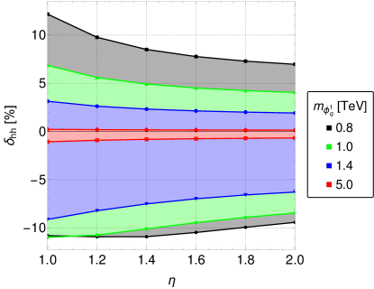
Figure 13: $\delta_{hh}$ as a function of the variable $\eta$ defined as $m_{\phi_{q}^{2}}=\eta\ m_{\phi_{q}^{1}}$. The plot is for $n=2$ and $\eta$ was varied between 1 and 2. This relaxes the condition of equal masses fixing $m_{\phi_{q}^{1}}$ while increasing $m_{\phi_{q}^{2}}$. The different colours represent the different values for the fixed mass, $m_{\phi_{q}^{1}}$.

3.5 Models with $n$ Coloured Scalars

We finalise this chapter by looking in more detail at double Higgs production in the case of an arbitrary number of scalars. The parameter space will be comprised of $n$ effective couplings $\lambda_{h\phi_{q}^{k}}$ to the Higgs boson and $n$ scalar masses $m_{\phi_{q}^{k}}^{2}$ ($k=1,...,n$), one for each of the coloured scalars, resulting in $2n$ input parameters ( $\lambda_{k}\equiv\lambda_{h\phi_{q}^{k}}$ from now on). We again start with the condition of equal masses, $m_{\phi_{q}^{k}}^{2}=m_{\phi_{q}^{l}}^{2}\equiv m_{\phi_{q}}^{2}$, reducing the input parameters to $n+1$. As discussed in the previous section, this condition should be sufficient in order to fully explore $\delta_{hh}$. For single Higgs production, this resulted in a simple dependence of the corrections on only the total sum of the couplings. In the case of Higgs pair production, the amplitude now contains both $\lambda_{k}$ and $\lambda_{k}^{2}$ terms and thus there are now two relevant quantities: the total sum of the couplings and the total sum of the squared couplings. Naturally, taking these two sums over the couplings as our parameters is advantageous, as it allows us to reduce the number of input parameters from $n+1$ to only 3, to properly study $\delta_{hh}$ for any model. The cases $n=1,2$ have two and three independent input parameters, respectively, and were studied in the previous sections.

We will now proceed to write both the cross section $\sigma_{hh}$ and the relative deviation from the SM cross section, $\delta_{hh}$, as a function of the two effective quantities, $\sum\lambda_{k}$ and $\sum\lambda_{k}^{2}$. Assuming a common fixed coloured mass $m_{\phi_{q}}^{2}$, as we do from now on, we note that because single Higgs production only depends on $\sum\lambda_{k}$, if one is able to write the relative deviations $\delta_{h,hh}$ as a function of the same variable, the two results can be combined. Even under the simplification of equal masses, we have now $\delta_{hh}$ as a function of two parameters, $\delta_{hh}\equiv\delta_{hh}\left(\sum\lambda_{k},\sum\lambda_{k}^{2}\right)$. Therefore, the model limits are represented by a 2-dimensional region in the parameter space of these two sums. By taking the approach where we consider the sum $\sum\lambda_{k}$ as the independent variable, the limits on this sum are easily obtained. Applying the same constraints, $\lambda_{min}\leq\lambda_{k}\leq\lambda_{max}$, to all the couplings of a model with $n$ coloured scalars, the sum of the couplings will be limited by

$$n\lambda_{min}\leq\sum\lambda_{k}\leq n\lambda_{max}\ .$$ (50)

As for the limits for $\sum\lambda_{k}^{2}$ as a function of $\sum\lambda_{k}$, we need to find the solution of a conditional extreme problem: the extremes of $\sum\lambda_{k}^{2}$ subject to the constraints $\sum\lambda_{k}=c$ and $\lambda_{min}\leq\lambda_{k}\leq\lambda_{max}$. Within the $n$ dimensional space of the individual couplings, $(\lambda_{1},\lambda_{2},...\lambda_{n})$, the region of interest is represented by an $n-1$ hyperplane defined by $\sum\lambda_{k}=c$ but constrained by an $n$-dimensional hypercube resulting from the constrained couplings, $\lambda_{min}\leq\lambda_{k}\leq\lambda_{max}$. For a fixed sum ($\sum\lambda_{k}=c$) the minimum of $\sum\lambda_{k}^{2}$ is given when the couplings are all equal

$$\sum\lambda_{k}^{2}\geq\frac{c^{2}}{n}=\frac{\left(\sum\lambda_{k}\right)^{2}}{n}\ ,$$ (51)

which is a just a Cauchy-Schwartz type of inequality.

The determination of the maximum is more elaborated. The solution is given by the edges of the hypercube or, more simply, when all but one coupling are fixed to $\lambda_{min}$ or $\lambda_{max}$. This can be cast in the form,

$$\sum_{k=1}^{n}\lambda_{k}^{2}\leq\sum_{j=0}^{n-1}\Bigg{\{}\left[j\lambda_{max}^{2}+\left(n-1-j\right)\lambda_{min}^{2}+\left(\sum_{k=1}^{n}\lambda_{k}-\left(j\lambda_{max}+\left(n-1-j\right)\lambda_{min}\right)\right)^{2}\right]\times\\ \left[\Theta\left(\sum_{k=1}^{n}\tilde{\lambda}_{k}-j\right)-\Theta\left(\sum_{k=1}^{n}\tilde{\lambda}_{k}-(j+1)\right)\right]\Bigg{\}}\ ,$$ (52)

where $\tilde{\lambda}_{k}=(\lambda_{k}-\lambda_{min})/(\lambda_{max}-\lambda_{min})$ and $\Theta(x)$ is the Heaviside function. The derivation of this formula can be found in [86].

In Fig. 14 we present an example of the region determined by the above conditions. We show the allowed regions for each model defined by the number $n$ of coloured scalars. The left plot depicts the borders of the labelled regions for even values of $n$. The odd values in-between are represented by a dashed grey line. The right plot focuses on the lower values of $n$, representing all up to $n=4$. Higher values are represented by grey dashed lines.

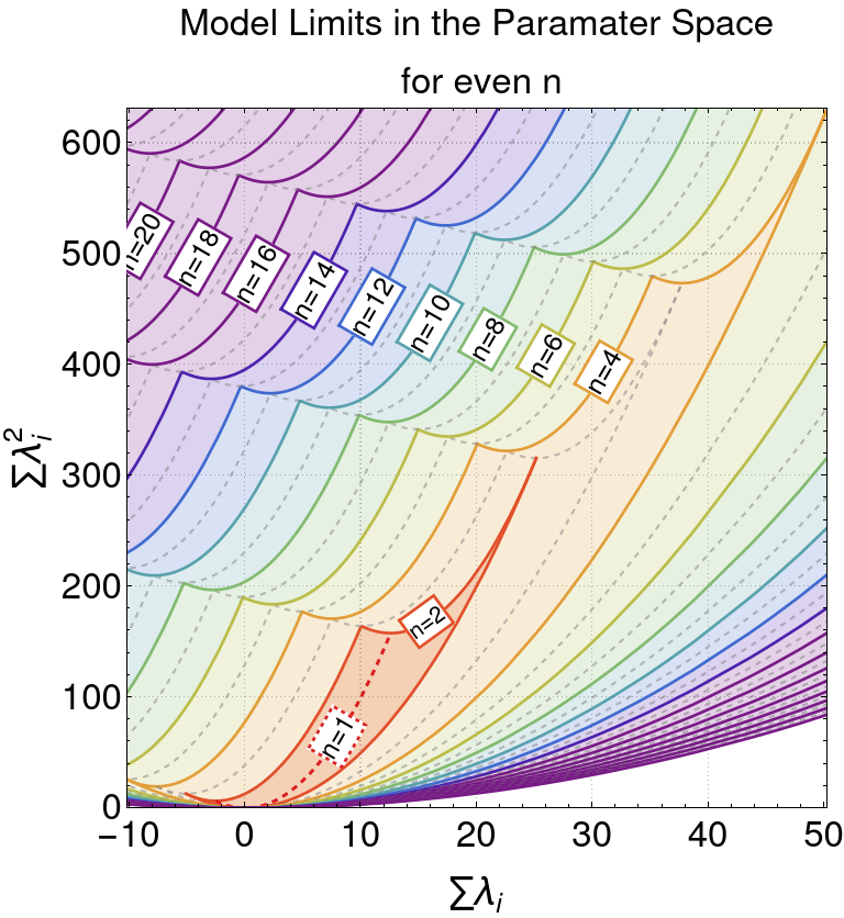
(a)

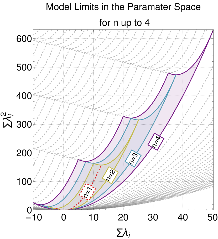
(b)

Figure 14: Allowed regions for each model defined by the number $n$ of coloured scalars. The left plot depicts the borders of the labelled regions for even values of $n$. The odd values in-between are represented by a dashed grey line. Of note is that, for $n=1$, the limits are not a region but just a single line (represented as a dashed red line). The right plot focuses on the lower values of $n$, representing all up to $n=4$. Higher values are represented by grey dashed lines.

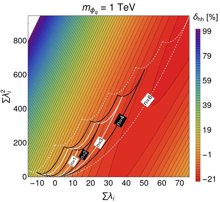
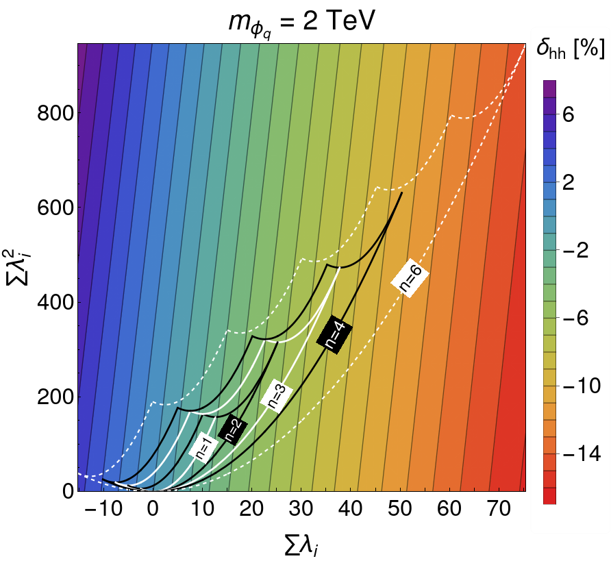
Figure 15: $\Sigma\lambda_{i}^{2}$ as a function of $\Sigma\lambda_{i}$ with the value of $\delta_{hh}$ in the colour bar. Left (right): $m_{\phi_{q}}=$ 1(2) TeV. Note that the colour scale is not the same in the two figures. The contours represent the allowed values for $\delta_{hh}$ for each value of $n$. The allowed region for $n=5$ has not been represented as it would make the identification of the $n=4$ and $n=6$ regions more difficult.

The next step is to calculate $\delta_{hh}$ as a function of the two sums $\sum\lambda_{k}$ and $\sum\lambda_{k}^{2}$. This can be done by discretising the two variables in $N$ points which would involve a computational time of $\mathcal{O}(N^{2})$. We will instead present an approach that can recycle the previous results from Fig. 11 with $n=2$ and a fixed mass, which can be computed in $\mathcal{O}(N)$ time. We separate the individual contributions to $\delta_{hh}$ into three components as follows:

$$\begin{array}[]{lll}\delta_{n,\text{ eq}}^{\ A}(\lambda):&\sim\{F_{\triangle}^{\phi_{q}},|F_{\triangle}^{\phi_{q}}|^{2},F_{\square_{2}}^{\phi_{q}},|F_{\square_{2}}^{\phi_{q}}|^{2},2\mbox{Re}(F_{\triangle}^{\phi_{q}}F_{\square_{2}}^{\phi_{q}*})\}&\sim\{G_{\phi_{q}}^{h},(G_{\phi_{q}}^{h})^{2},G_{\phi_{q}}^{hh},(G_{\phi_{q}}^{hh})^{2},G_{\phi_{q}}^{h}\cdot G_{\phi_{q}}^{hh}\}\\ \delta_{n,\text{ eq}}^{\ B}(\lambda):&\sim\{F_{\square_{1}}^{\phi_{q}},G_{\square_{1}}^{\phi_{q}},|F_{\square_{1}}^{\phi_{q}}|^{2},|G_{\square_{1}}^{\phi_{q}}|^{2}\}&\sim\{G_{\phi_{q}}^{h,\,2},G_{\phi_{q}}^{h,\,2},(G_{\phi_{q}}^{h,\,2})^{2},(G_{\phi_{q}}^{h,\,2})^{2}\}\\ \delta_{n,\text{ eq}}^{\ C}(\lambda):&\sim\{2\mbox{Re}(F_{\triangle}^{\phi_{q}}F_{\square_{1}}^{\phi_{q}*}),2\mbox{Re}(F_{\square_{1}}^{\phi_{q}}F_{\square_{2}}^{\phi_{q}*})\}&\sim\{G_{\phi_{q}}^{h}\cdot G_{\phi_{q}}^{h,\,2},G_{\phi_{q}}^{h,\,2}\cdot G_{\phi_{q}}^{hh}\}\end{array}$$ (56)

where the label "eq" indicates the equal coupling condition ($\lambda_{k}=\lambda_{l}\equiv\lambda$) and there is only one independent parameter, $\lambda$, due to this condition. We have already found that all three components can be significant and must be taken into account. The equivalence between these three components for a model with $n$ couplings with an arbitrary model with $n^{\prime}$ couplings, $\{\lambda^{\prime}_{1},...,\lambda^{\prime}_{n^{\prime}}\}$, is given by the following formula:

$$\delta^{n^{\prime}}_{hh}(\{\lambda^{\prime}_{1},...,\lambda^{\prime}_{n^{\prime}}\})=\delta_{n,\text{ eq}}^{A}(\lambda)\bigg{\rvert}_{\lambda=\frac{1}{n}\sum\lambda^{\prime}_{k}}+\delta_{n,\text{ eq}}^{B}(\lambda)\bigg{\rvert}_{\lambda=\sqrt{\frac{1}{n}\sum\lambda_{k}^{{}^{\prime}2}}}+\delta_{n,\text{ eq}}^{C}(\lambda)\bigg{\rvert}_{\lambda=\sqrt[3]{\left(\frac{1}{n}\sum\lambda^{\prime}_{k}\right)\left(\frac{1}{n}\sum\lambda_{k}^{{}^{\prime}2}\right)}}\ \ \ .$$ (57)

In other words, the $\delta_{hh}^{n^{\prime}}$ for a model with $n^{\prime}$ couplings can be obtained from the results for a model with $n$ equal couplings $\lambda$, by taking the $A$, $B$, and $C$ contributions at the $\lambda$ values indicated by the vertical bars.

In Fig. 15 we show $\Sigma\lambda_{i}^{2}$ as a function of $\Sigma\lambda_{i}$ with the value of $\delta_{hh}$ in the colour bar. The left plot is for a coloured scalar mass of 1 TeV while the right plot is for 2 TeV. Note that the colour scale is not the same in the two figures. The contours represent the allowed values for $\delta_{hh}$ for each value of $n$. The comparison of the two plots shows that, as expected, the range of variation of $\delta_{hh}$ decreases with increasing value of $m_{\phi_{q}}$. Furthermore, the dependence of $\delta_{hh}$ on $\sum\lambda_{k}^{2}$ decreases with increasing coloured mass which is due to the fact that the terms proportional to $\sum\lambda_{k}^{2}$ are suppressed by a factor of $1/m_{\phi_{q}}^{4}$.

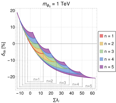
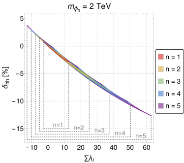
Figure 16: $\delta_{hh}$ for a scalar mass of 1 TeV (left) and 2 TeV (right) as a function of $\sum\lambda_{i}$. This encompasses the possible range from the freedom in $\sum\lambda_{i}^{2}$ and was calculated with the results and model limits from Figure 15.

In Fig. 16 we now show $\delta_{hh}$ as a function of the sum of couplings, $\sum\lambda_{k}$. The range of variation is related with the freedom in $\sum\lambda_{k}^{2}$ and was calculated with the results and model limits from Fig. 15. As the mass grows the term in $\lambda_{k}$ becomes increasingly important and for a mass of 2 TeV the variation in $\lambda_{k}^{2}$ almost vanishes. Therefore, for large masses the dependence for single and double Higgs productions becomes very similar. Note, that since the interference is destructive for positive couplings in the case of double Higgs production, the maximum $\delta_{hh}$ occurs for the smaller (negative) values of the couplings.

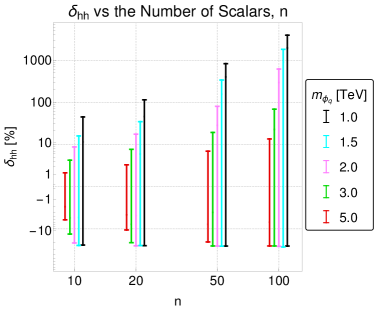
Figure 17: $\delta_{hh}$ as a function of the number of scalars $n$ for three (left) and five (right) coloured scalar masses with $n=1,...,10$ (left) and $n=10,20,50,100$ (right).

Finally, in Fig. 17 left (right) we present $\delta_{hh}$ as a function of the number of scalars $n$ for three (five) coloured scalar masses. The left plot shows the scenarios from $n=1$ to $n=10$ while the right plot shows larger values of $n$. For small $n$ the deviations from the SM are small as we had seen before but they can be extremely large for very large values of $n$, even if the coloured scalar masses are large.

Contrary to single Higgs production, the experimental limits on double Higgs production are very weak and at the moment unlikely to be useful in constraining the parameter space. The lowest observed bound on the limit for double Higgs production, as reported by the ATLAS collaboration to be 6.9 times the SM cross section, is equivalent to a $\delta_{hh}$ of $590\%$ [87] for a c.m. energy of 13 TeV. With a mass of 1 TeV, this would apply constraints only above $n\approx 45$. As for possible future improvements we can consider the HL-LHC projections [60]. For the $hh\rightarrow b\bar{b}b\bar{b}$ channel a reported value as low as 1.6 times the SM cross section, equivalent to a $\delta_{hh}$ of $60\%$, can be achieved, assuming that the overall uncertainty scales with the luminosity as $1/\sqrt{L}$. This would bring the previous threshold value of $n$ down to around 13. This means that certain combinations of the masses with the number of scalars will certainly be constrained with future measurements.

4 Single Higgs vs. Double Higgs Production

In the previous chapters we have discussed in detail the contribution of an arbitrary number of coloured scalars to single Higgs and di-Higgs production processes via gluon fusion at the LHC. We will now discuss the complementarity between the two processes. One should note, however, that although we expect a good precision in the measurement of the single Higgs process this is not the case for di-Higgs production.

The first point to note is that the NP contribution to the single Higgs mode has a constructive interference for positive $\lambda_{k}$ while for di-Higgs it is negative. The reason for the positive interference term for $\lambda_{k}>0$, is that both the SM and the NP form factors in single Higgs production are positive. For double Higgs production this is no longer the case. The reason behind this is the destructive interferences between the ($F_{\triangle}^{Q/\phi_{q}}$, $F_{\square_{2}}^{\phi_{q}}$) and ($F_{\square}^{Q}$,$F_{\square_{1}}^{\phi_{q}}$) form factors. It is already well known that the SM triangle and box form factors interfere destructively as can be read off from their values in the heavy quark limit, $F_{\triangle}^{Q}=\frac{2}{3}+\mathcal{O}(m_{Q}^{-2})$ and $F_{\square}^{Q}=-\frac{2}{3}+\mathcal{O}(m_{Q}^{-2})$. To understand why this also applies to our coloured scalars we can make use of the Low Energy Theorem as was done in [88, 89] (for squarks) to deduce the sign of $F_{\square_{1}}^{\phi_{q}}$. By this theorem, $F_{\square_{1}}^{\phi_{q}}$ is given by the derivative in mass of the term $F_{\triangle}^{\phi_{q}}/m_{\phi_{q}}^{2}$. Since we already know that the triangle form factor for large scalar masses decreases with the mass, the sign of $F_{\square_{1}}^{\phi_{q}}$ will be negative. Therefore the negative contributions for positive couplings we are observing are due to the interference terms of the NP form factors, $F_{\triangle}^{\phi_{q}}\cdot F_{\square_{1}}^{\phi_{q}}$ and $F_{\square_{2}}^{\phi_{q}}\cdot F_{\square_{1}}^{\phi_{q}}$, but also from the interference between SM and NP form factors, $F_{\square}^{Q}\cdot F_{\triangle}^{\phi_{q}}$, $F_{\square}^{Q}\cdot F_{\square_{2}}^{\phi_{q}}$ and $F_{\triangle}^{Q}\cdot F_{\square_{1}}^{\phi_{q}}$. The remaining $F\cdot F$ terms involving at least one NP form factor are positive. As for $G_{\square}^{Q}\cdot G_{\square_{1}}^{\phi_{q}}$, its contribution to the amplitude is suppressed by $(1/m_{Q}^{2})\cdot(1/m_{\phi_{q}}^{6})$, where the latter factor stems from the $G_{\square_{1}}^{\phi_{q}}$ dependence $\sim 1/m_{\phi_{q}}^{2}$ multiplied by the coupling factor $(g_{\phi_{q}}^{h})^{2}\sim 1/m_{\phi_{q}}^{4}$.

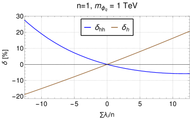
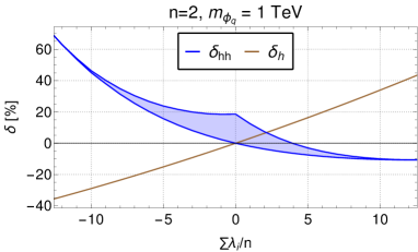
Figure 18: $\delta_{hh}$ (blue) and $\delta_{h}$ (brown) as a function of the averaged coupling for $n=1$ (left) and for $n=2$ (right). For these plots only, the minimum coupling used was $-4\pi$ instead of the previous bounded-from-below condition.

In Fig. 18 we present $\delta_{hh}$ (blue) and $\delta_{h}$ (brown) as a function of the averaged coloured coupling $\sum\lambda_{k}/n$ for $n=1$ (left) and $n=2$ (right). The mass of the coloured scalars has been chosen equal and set to 1 TeV. We note that with the chosen input values given above we obtain at $\sqrt{s}=14$ TeV at LO for the SM the single Higgs cross section value $\sigma^{h}_{SM}=15.76$ pb calculated with HIGLU including the bottom, charm and top quark loops, and the double Higgs cross section value $\sigma^{hh}_{SM}=16.37$ fb calculated with HPAIR including the bottom and top quark loops. The complementarity between the dependence of $\delta_{h}$ and $\delta_{hh}$ w.r.t. the coupling $\lambda_{k}$ is very clear from the figure. We also note that for $n=1$ the $\delta_{h}$ and $\delta_{hh}$ values are lines while for $n=2$ there is an allowed region for $\delta_{hh}$ due to the additional dependence on $\sum_{k}\lambda_{k}^{2}$. This leads to the observation that, with a single Higgs measurement very close to the SM value constraining $\sum\lambda_{k}/n$ to small values, any significant excess of di-Higgs production would provide a strong indication that $n\geq 2$.

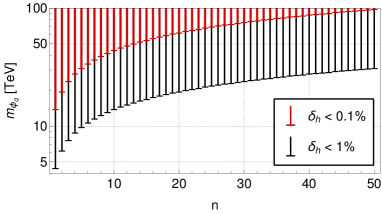
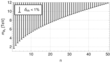
Figure 19: Regions where $\delta_{h}$ (left) and $\delta_{hh}$ (right) fall below 1% as a function of the coloured scalar mass and the number of scalars. For the single Higgs production (left) the threshold of 0.1% has also been included. For these calculations the previous BFB condition from Eq. (20) was used.

We finalise this section with a plot (Fig. 19) where we show the region of the coloured mass versus the number of scalars that leads to a maximal deviation of 1% (black) or 0.1% (red) in $\delta_{h}$ (left) and to a maximal deviation of 1% in $\delta_{hh}$ (right) of single, respectively, double Higgs production from the corresponding SM value, while varying the couplings within their allowed theoretical bounds. This gives us a feeling on the region where it will not be possible to probe these models even in the long run. For double Higgs production we indicate the 1% region only, since the predictions for the HL-LHC are significantly above this threshold ($\delta_{hh}^{\text{HL-LHC}}=60\%$). For the single Higgs production, the predictions ($\delta_{h}^{\text{HL-LHC}}=1.6\%$) indicate that a precision of 1% could be attainable. Thus we also present the 0.1% region in this case as the region that cannot be probed by experiment. As single Higgs production can be constrained more stringently (possibly up to 0.1%) than Higgs pair production this means that larger coloured masses can be probed in single than in di-Higgs production. Independently of the experimental precisions, the plots show, that single Higgs production is more sensitive to coloured scalars than di-Higgs production. For a value of $n=10$ e.g. a value of $\delta_{h}=1$% probes masses of about 12 TeV, whereas $\delta_{hh}=1$% probes masses of 5 TeV only. Finally, we have checked that the lower border of the regions, where $\delta=1\%$ or $0.1\%$, follows the relationship $n\propto m_{\phi_{q}}^{2}$ very closely. The large masses required for these low values of $\delta$ ensure that the terms proportional to $n/m_{\phi_{q}}^{2}$ are dominant and hence why this behaviour is observed.

5 Conclusions

We have calculated the relative changes $\delta_{h}$ of SM single and $\delta_{hh}$ of SM double Higgs production when including new heavy coloured scalars. Our calculations are based on the LO cross sections at the LHC using the Fortran codes HIGLU and HPAIR where we included our new physics contributions. We have found that for an arbitrary number of scalars and taking their masses to be equal $\delta_{h}$ can be written as a function of only two variables, given by the sum of the couplings of the coloured particles to the Higgs boson, $\sum_{i}\lambda_{i}$, and their masses $m_{i}$. As for the double Higgs case, the $\delta_{hh}$ dependence extends now to three variables, the extra variable being $\sum_{i}\lambda_{i}^{2}$. We devised a way to find the limits on this new variable in terms of $\sum_{i}\lambda_{i}$, again for equal masses. We have discussed the limits on these variables for single Higgs production, where the results already constrain some of the parameter space. For di-Higgs production the bounds are still very loose and we have to wait until the end of Run3 to hopefully get some bounds on the couplings.

We have shown that if we relax the condition of equal masses what can be said is that the range of allowed values for $\delta_{hh}$ would be smaller than the range obtained by taking all masses equal to the smallest mass of the $n$ coloured scalars. We have also shown that taking equal couplings and performing a scan between their minimum and maximum values is sufficient to obtain the complete range for $\delta_{hh}$.

Another important point to note is the complementarity between single and di-Higgs processes. Once the value of the coupling is fixed, the relative deviations from the SM move in different directions. That is, if $\delta_{h}$ increases $\delta_{hh}$ decreases with the coupling and vice-versa. The extra freedom of $\delta_{hh}$ also provides another venue for determining the number of scalars from observations. An excess of single or di-Higgs production could indicate the existence of $n\geq 1$ coloured scalars. But an excess of di-Higgs production paired with a single Higgs measurement close to zero would point to $n>1$.

One final and very important point to note is that in direct searches for DM at the LHC we do not have access to the number of DM fields because we only look for missing energy associated with some SM particle. On the contrary, in our approach the number of fields is a variable that influences the results.

Appendix A HPAIR Extension to Coloured Scalars

In the following we present our implementation of the contributions from the coloured scalars to Higgs pair production at leading order in the code HPAIR. It has been made available at [90]. All changes of the original source code are contained entirely within hpair.f. The code is compiled by using make and then running the executable run which will assume the input and output files hpair.in and hpair.out respectively. For the compilation process the LHAPDF libraries required by HPAIR must be supplied and their installation path indicated with the variable LIBS in the makefile.

The BDM input options are contained within the original input file of HPAIR, hpair.in. The following lines delimit where these new options are found:

⬇

156!————————————————–

157!BDM OPTIONS:

158!=======================

159(…)

190!———————————BDM OPTIONS END—

By setting the variable ibdm to 1, the coloured scalar form factors are added to the SM amplitude. The type of model, characterised by the number of scalars $n$, is selected with the variable ibdmtype. These are found in the following block:

⬇

159!IF ibdm=1 THEN THE NEW SCALARS DIAGRAMS WILL BE ADDED TO F1

160ibdm = 1

161!SELECT BDM MODEL: 1 - Model n=1, 2 - Model n=2, 3 - Model n >= 2 with equal couplings and equal masses

162ibdmtype = 1

When ibdmtype is set to either 1 or 2, this corresponds to a model with 1 or 2 scalars, respectively. For each model type the masses in GeV, mphiq, and couplings to the Higgs, lambHPQ, must be supplied. These input parameters are set in the following blocks:

⬇

164!MODEL (n=1) PARAMETERS:

165mphiq1 = 2000.D0

166lambHPQ1 = 1.0D0

167

168!MODEL (n=2) PARAMETERS:

169mphiq1 = 1000.D0

170mphiq2 = 1000.D0

171lambHPQ1 = 1.000D0

172lambHPQ2 = 1.000D0

On the other hand, setting ibdmtype to 3, allows for a model with a generic number of scalars $n$. This comes with the limitation that all the scalars must have the same mass, mphiq1, and coupling, lambHPQ1. These 3 input parameters can be set in the following block:

⬇

174!MODEL (n>=2) PARAMETERS:

175mphiq1 = 1200.D0

176lambHPQ1 = 12.D0

177Nscalars = 2

The final block of parameters relates to the individual form factor selection and it applies to all the three options for ibdmtype. The relevant lines are:

⬇

179!DIAGRAMS/FORM FACTORS SELECTION:

180!IF FULL=1 THEN FULL FORMULA IS USED INSTEAD

181full = 1

182triang = 1

183boxTri = 1

184boxQuad = 0

The variable full is used to select whether all the NP form factors, as presented in Eqs. (27) and (29), are automatically included in the amplitude (full=1) or not (full=0). In the latter case, the following three variables triang, boxTri and boxQuad are used to determine which form factors are to be included in the calculations:

• triang=1: Will include the triangle form factor $g_{\phi_{q}}^{h}F_{\triangle}^{\phi_{q}}$ (Eq. (5)) originating from the triangle diagrams (Fig. 7(b)-7(c))

• boxTri=1: Will include the box form factors $(g_{\phi_{q}}^{h})^{2}G_{\square_{1}}^{\phi_{q}}$ and $(g_{\phi_{q}}^{h})^{2}F_{\square_{1}}^{\phi_{q}}$ (Eqs. (31–32)) originating from the box diagrams with the triple couplings between one Higgs and two coloured scalars (Fig. 8(b)-8(c))

• boxQuad=1: Will include the box form factor $(g_{\phi_{q}}^{hh})F_{\square_{2}}^{\phi_{q}}$ (Eq. (5), as $F_{\square_{2}}^{\phi_{q}}=F_{\triangle}^{\phi_{q}}$) originating from the box diagrams with the quartic couplings between two Higgs and two coloured scalars (Fig. 8(d)-8(e))

Some care in the formatting must be taken when changing the values of the parameters. The code uses the number of the lines to identify the input parameters and thus they must be preserved. The names of the variables indicated in the input file have no impact. However, the number of characters before the equal sign must always be nine in total:

⬇

179$\underbrace{\text{ibdm\textvisiblespace\textvisiblespace\textvisiblespace\textvisiblespace\textvisiblespace}}_{\text{9 charaters}}$= 1

These considerations are important to keep in mind when using a script to automatically change the input values.

The output file suffers no changes from the original HPAIR template, hpair.out. The NP contributions only affect the LO cross section which can be extracted from the following line:

⬇

SIGMA_BORN = ( 2.0478260337291408E-002 +- 2.4261364431116920E-005 ) PB

Appendix B Double Higgs Production

For completeness, we repeat here the SM box form factors appearing in Eq. (29), which can also be found e.g. in [62]. They are given by:

$$F_{\square}^{Q}=\frac{2m_{Q}^{2}}{s}\Bigg{(}2+(4m_{Q}^{2})C_{ab}^{m_{Q}^{2}}+\frac{2}{s}(t-m_{h}^{2})(m_{h}^{2}-4m_{Q}^{2})C_{ac}^{m_{Q}^{2}}\\ +\frac{2}{s}(u-m_{h}^{2})(m_{h}^{2}-4m_{Q}^{2})C_{bc}^{m_{Q}^{2}}-m_{Q}^{2}(s+2m_{h}^{2}-8m_{Q}^{2})(D_{abc}^{m_{Q}^{2}}+D_{bac}^{m_{Q}^{2}})\\ +(m_{Q}^{2}(s+2m_{h}^{2}-8m_{Q}^{2})-\frac{1}{s}(m_{h}^{2}-4m_{Q}^{2})(tu-m_{h}^{4}))D_{acb}^{m_{Q}^{2}}\Bigg{)}\ ,$$ (58)

$$G_{\square}^{Q}=\frac{2m_{Q}^{2}}{s}\left(\frac{1}{tu-m_{h}^{4}}\right)\Bigg{(}\frac{s}{2}(t^{2}+u^{2}+2m_{h}^{4}-8m_{Q}^{2}(t+u))C_{ab}^{m_{Q}^{2}}\\ +(t^{2}+m_{h}^{4}-8tm_{Q}^{2})(t-m_{h}^{2})C_{ac}^{m_{Q}^{2}}+(u^{2}+m_{h}^{4}-8um_{Q}^{2})(u-m_{h}^{2})C_{bc}^{m_{Q}^{2}}\\ -\frac{1}{2}(t^{2}+u^{2}-2m_{h}^{4})(t+u-8m_{Q}^{2})C_{cd}^{m_{Q}^{2}}\\ -(st(t^{2}/2+m_{h}^{4}/2-4tm_{Q}^{2})+m_{Q}^{2}(t+u-8m_{Q}^{2})(tu-m_{h}^{4}))D_{bac}^{m_{Q}^{2}}\\ -(su(u^{2}/2+m_{h}^{4}/2-4um_{Q}^{2})+m_{Q}^{2}(t+u-8m_{Q}^{2})(tu-m_{h}^{4}))D_{abc}^{m_{Q}^{2}}\\ -m_{Q}^{2}(t+u-8m_{Q}^{2})(tu-m_{h}^{4})D_{acb}^{m_{Q}^{2}}\Bigg{)}\ ,$$ (59)

where the Mandelstam variables $s,t,u$ are defined as:

$$s=(p_{a}+p_{b})^{2}\ ,\quad t=(p_{a}-p_{c})^{2}\ ,\quad u=(p_{b}-p_{c})^{2}\ .$$ (60)

They also involve the following scalar integrals:

$$C_{ab}=\int\frac{d^{4}q}{i\pi^{2}}\frac{1}{\left(q^{2}-m_{X}^{2}\right)\left((q+p_{a})^{2}-m_{X}^{2}\right)\left((q+p_{a}+p_{b})^{2}-m_{X}^{2}\right)}\ ,$$ (61)

$$D_{abc}=\int\frac{d^{4}q}{i\pi^{2}}\frac{1}{\left(q^{2}-m_{X}^{2}\right)\left((q+p_{a})^{2}-m_{X}^{2}\right)\left((q+p_{a}+p_{b})^{2}-m_{X}^{2}\right)\left((q+p_{a}+p_{b}+p_{c})^{2}-m_{X}^{2}\right)}\ ,$$ (62)

where $X$ stands for the quark or coloured scalar as appropriate. The exact formula for $C_{ab}$ has been determined and is given by:

$$C_{ab}=-\frac{2}{s}f(\tau)\ ,$$ (63)

where $f_{\tau}$ is given in Eq. (6) and $\tau=\frac{4m_{X}^{2}}{s}$.

Acknowledgements

PG is supported by the Portuguese Foundation for Science and Technology (FCT) with a PhD Grant No. 2022.11377.BD. PG, DN and RS are partially supported by FCT under Contracts no. UIDB/00618/2020, UIDP/00618/2020, PTDC/FIS-PAR/31000/2017 and CERN/FIS-PAR/0014 /2019. The work of MM is supported by the DFG Collaborative Research Center TRR257 “Particle Physics Phenomenology after the Higgs Discovery”.

References

- [1] LHCb collaboration, R. Aaij et al., Test of lepton universality in beauty-quark decays, Nature Phys. 18 (2022) 277–282, [2103.11769].
- [2] LHCb collaboration, R. Aaij et al., Search for lepton-universality violation in decays, Phys. Rev. Lett. 122 (2019) 191801, [1903.09252].
- [3] Muon g-2 collaboration, D. P. Aguillard et al., Measurement of the Positive Muon Anomalous Magnetic Moment to 0.20 ppm, 2308.06230.
- [4] Particle Data Group collaboration, M. Tanabashi et al., Review of Particle Physics, Phys. Rev. D 98 (2018) 030001.
- [5] T. P. Gorringe and D. W. Hertzog, Precision Muon Physics, Prog. Part. Nucl. Phys. 84 (2015) 73–123, [1506.01465].
- [6] T. Aoyama et al., The anomalous magnetic moment of the muon in the Standard Model, Phys. Rept. 887 (2020) 1–166, [2006.04822].
- [7] Muon g-2 collaboration, G. W. Bennett et al., Final Report of the Muon E821 Anomalous Magnetic Moment Measurement at BNL, Phys. Rev. D 73 (2006) 072003, [hep-ex/0602035].
- [8] LHCb collaboration, Measurement of lepton universality parameters in and decays, 2212.09153.
- [9] LHCb collaboration, Test of lepton universality in decays, 2212.09152.
- [10] D. Huang, A. P. Morais and R. Santos, Anomalies in -meson decays and the muon from dark loops, Phys. Rev. D 102 (2020) 075009, [2007.05082].
- [11] R. Capucha, D. Huang, T. Lopes and R. Santos, Impact of electroweak group representation in models for B and g-2 anomalies from dark loops, Phys. Rev. D 106 (2022) 095032, [2207.11556].
- [12] D. G. Cerdeño, A. Cheek, P. Martín-Ramiro and J. M. Moreno, B anomalies and dark matter: a complex connection, Eur. Phys. J. C 79 (2019) 517, [1902.01789].
- [13] ATLAS collaboration, M. Aaboud et al., Search for dark matter produced in association with bottom or top quarks in TeV pp collisions with the ATLAS detector, Eur. Phys. J. C 78 (2018) 18, [1710.11412].
- [14] H. M. Georgi, S. L. Glashow, M. E. Machacek and D. V. Nanopoulos, Higgs Bosons from Two Gluon Annihilation in Proton Proton Collisions, Phys. Rev. Lett. 40 (1978) 692.
- [15] M. Spira, Higgs Boson Production and Decay at Hadron Colliders, Prog. Part. Nucl. Phys. 95 (2017) 98–159, [1612.07651].
- [16] M. Spira, HIGLU: A program for the calculation of the total Higgs production cross-section at hadron colliders via gluon fusion including QCD corrections, hep-ph/9510347.
- [17] A. Djouadi, M. Spira and P. Zerwas, Production of Higgs bosons in proton colliders. QCD corrections, Physics Letters B 264 (1991) 440–446.
- [18] S. Dawson, Radiative corrections to Higgs boson production, Nuclear Physics B 359 (1991) 283–300.
- [19] D. Graudenz, M. Spira and P. M. Zerwas, QCD corrections to Higgs boson production at proton proton colliders, Phys. Rev. Lett. 70 (1993) 1372–1375.
- [20] M. Spira, A. Djouadi, D. Graudenz and P. M. Zerwas, Higgs boson production at the LHC, Nucl. Phys. B 453 (1995) 17–82, [hep-ph/9504378].
- [21] R. Harlander and P. Kant, Higgs production and decay: Analytic results at next-to-leading order QCD, JHEP 12 (2005) 015, [hep-ph/0509189].
- [22] C. Anastasiou, S. Beerli, S. Bucherer, A. Daleo and Z. Kunszt, Two-loop amplitudes and master integrals for the production of a Higgs boson via a massive quark and a scalar-quark loop, JHEP 01 (2007) 082, [hep-ph/0611236].
- [23] U. Aglietti, R. Bonciani, G. Degrassi and A. Vicini, Analytic Results for Virtual QCD Corrections to Higgs Production and Decay, JHEP 01 (2007) 021, [hep-ph/0611266].
- [24] C. Anastasiou, S. Bucherer and Z. Kunszt, HPro: A NLO Monte-Carlo for Higgs production via gluon fusion with finite heavy quark masses, JHEP 10 (2009) 068, [0907.2362].
- [25] S. Catani, D. de Florian and M. Grazzini, Higgs production in hadron collisions: Soft and virtual QCD corrections at NNLO, JHEP 05 (2001) 025, [hep-ph/0102227].
- [26] R. V. Harlander and W. B. Kilgore, Soft and virtual corrections to proton proton — H + x at NNLO, Phys. Rev. D 64 (2001) 013015, [hep-ph/0102241].
- [27] R. V. Harlander and W. B. Kilgore, Next-to-next-to-leading order Higgs production at hadron colliders, Phys. Rev. Lett. 88 (2002) 201801, [hep-ph/0201206].
- [28] C. Anastasiou and K. Melnikov, Higgs boson production at hadron colliders in NNLO QCD, Nucl. Phys. B 646 (2002) 220–256, [hep-ph/0207004].
- [29] V. Ravindran, J. Smith and W. van Neerven, NNLO corrections to the total cross section for Higgs boson production in hadron-hadron collisions, Nuclear Physics B 665 (2003) 325–366.
- [30] S. Marzani, R. D. Ball, V. Del Duca, S. Forte and A. Vicini, Higgs production via gluon-gluon fusion with finite top mass beyond next-to-leading order, Nuclear Physics B 800 (2008) 127–145.
- [31] T. Gehrmann, M. Jaquier, E. W. N. Glover and A. Koukoutsakis, Two-Loop QCD Corrections to the Helicity Amplitudes for 3 partons, JHEP 02 (2012) 056, [1112.3554].
- [32] C. Anastasiou, C. Duhr, F. Dulat and B. Mistlberger, Soft triple-real radiation for Higgs production at N3LO, JHEP 07 (2013) 003, [1302.4379].
- [33] C. Anastasiou, C. Duhr, F. Dulat, F. Herzog and B. Mistlberger, Real-virtual contributions to the inclusive Higgs cross-section at , JHEP 12 (2013) 088, [1311.1425].
- [34] W. B. Kilgore, One-loop single-real-emission contributions to at next-to-next-to-next-to-leading order, Phys. Rev. D 89 (2014) 073008, [1312.1296].
- [35] Y. Li, A. von Manteuffel, R. M. Schabinger and H. X. Zhu, N3LO Higgs boson and Drell-Yan production at threshold: The one-loop two-emission contribution, Phys. Rev. D 90 (2014) 053006, [1404.5839].
- [36] C. Anastasiou, C. Duhr, F. Dulat, E. Furlan, T. Gehrmann, F. Herzog et al., Higgs Boson GluonFfusion Production Beyond Threshold in N QCD, JHEP 03 (2015) 091, [1411.3584].
- [37] C. Anastasiou, C. Duhr, F. Dulat, F. Herzog and B. Mistlberger, Higgs Boson Gluon-Fusion Production in QCD at Three Loops, Phys. Rev. Lett. 114 (2015) 212001, [1503.06056].
- [38] C. Anastasiou, C. Duhr, F. Dulat, E. Furlan, T. Gehrmann, F. Herzog et al., High precision determination of the gluon fusion Higgs boson cross-section at the LHC, JHEP 05 (2016) 058, [1602.00695].
- [39] B. Mistlberger, Higgs boson production at hadron colliders at N3LO in QCD, JHEP 05 (2018) 028, [1802.00833].
- [40] C. Duhr, B. Mistlberger and G. Vita, Soft integrals and soft anomalous dimensions at N3LO and beyond, JHEP 09 (2022) 155, [2205.04493].
- [41] J. Baglio, C. Duhr, B. Mistlberger and R. Szafron, Inclusive production cross sections at N3LO, JHEP 12 (2022) 066, [2209.06138].
- [42] R. V. Harlander and K. J. Ozeren, Top mass effects in Higgs production at next-to-next-to-leading order QCD: Virtual corrections, Phys. Lett. B 679 (2009) 467–472, [0907.2997].
- [43] R. V. Harlander and K. J. Ozeren, Finite top mass effects for hadronic Higgs production at next-to-next-to-leading order, JHEP 11 (2009) 088, [0909.3420].
- [44] R. V. Harlander, H. Mantler, S. Marzani and K. J. Ozeren, Higgs production in gluon fusion at next-to-next-to-leading order QCD for finite top mass, Eur. Phys. J. C 66 (2010) 359–372, [0912.2104].
- [45] A. Pak, M. Rogal and M. Steinhauser, Finite top quark mass effects in NNLO Higgs boson production at LHC, JHEP 02 (2010) 025, [0911.4662].
- [46] A. Djouadi and P. Gambino, Leading electroweak correction to Higgs boson production at proton colliders, Phys. Rev. Lett. 73 (1994) 2528–2531, [hep-ph/9406432].
- [47] K. G. Chetyrkin, B. A. Kniehl and M. Steinhauser, Three loop O (alpha-s**2 G(F) M(t)**2) corrections to hadronic Higgs decays, Nucl. Phys. B 490 (1997) 19–39, [hep-ph/9701277].
- [48] K. G. Chetyrkin, B. A. Kniehl and M. Steinhauser, Virtual top quark effects on the H — b anti-b decay at next-to-leading order in QCD, Phys. Rev. Lett. 78 (1997) 594–597, [hep-ph/9610456].
- [49] G. Degrassi and F. Maltoni, Two-loop electroweak corrections to Higgs production at hadron colliders, Phys. Lett. B 600 (2004) 255–260, [hep-ph/0407249].
- [50] U. Aglietti, R. Bonciani, G. Degrassi and A. Vicini, Two-loop electroweak corrections to Higgs production in proton-proton collisions, in TeV4LHC Workshop: 2nd Meeting, 10, 2006. hep-ph/0610033.
- [51] S. Actis, G. Passarino, C. Sturm and S. Uccirati, NLO Electroweak Corrections to Higgs Boson Production at Hadron Colliders, Phys. Lett. B 670 (2008) 12–17, [0809.1301].
- [52] S. Actis, G. Passarino, C. Sturm and S. Uccirati, NNLO Computational Techniques: The Cases H — gamma gamma and H — g g, Nucl. Phys. B 811 (2009) 182–273, [0809.3667].
- [53] C. Anastasiou, R. Boughezal and F. Petriello, Mixed QCD-electroweak corrections to Higgs boson production in gluon fusion, JHEP 04 (2009) 003, [0811.3458].
- [54] J. Butterworth et al., PDF4LHC recommendations for LHC Run II, J. Phys. G 43 (2016) 023001, [1510.03865].
- [55] NNPDF collaboration, R. D. Ball et al., The path to proton structure at 1% accuracy, Eur. Phys. J. C 82 (2022) 428, [2109.02653].
- [56] A. Crivellin and L. Schnell, Complete Lagrangian and set of Feynman rules for scalar leptoquarks, Comput. Phys. Commun. 271 (2022) 108188, [2105.04844].
- [57] P. M. Ferreira, R. Santos and A. Barroso, Stability of the tree-level vacuum in two Higgs doublet models against charge or CP spontaneous violation, Phys. Lett. B 603 (2004) 219–229, [hep-ph/0406231].
- [58] ATLAS collaboration, G. Aad et al., Combined measurements of Higgs boson production and decay using up to fb-1 of proton-proton collision data at 13 TeV collected with the ATLAS experiment, Phys. Rev. D 101 (2020) 012002, [1909.02845].
- [59] CMS collaboration, A. M. Sirunyan et al., Combined measurements of Higgs boson couplings in proton–proton collisions at , Eur. Phys. J. C 79 (2019) 421, [1809.10733].
- [60] M. Cepeda, S. Gori, P. Ilten, M. Kado, F. Riva, R. A. Khalek et al., Higgs physics at the HL-LHC and HE-LHC, 1902.00134.
- [61] E. W. N. Glover and J. J. van der Bij, HIGGS BOSON PAIR PRODUCTION VIA GLUON FUSION, Nucl. Phys. B 309 (1988) 282–294.
- [62] T. Plehn, M. Spira and P. M. Zerwas, Pair production of neutral Higgs particles in gluon-gluon collisions, Nucl. Phys. B 479 (1996) 46–64, [hep-ph/9603205].
- [63] T. Hahn, Generating feynman diagrams and amplitudes with FeynArts 3, Computer Physics Communications 140 (2001) 418–431.
- [64] Thomas Hahn, “FeynArts 3.11 User’s Guide.” https://feynarts.de/FA3Guide.pdf, (accessed 2023-07-26).
- [65] G. D. Kribs and A. Martin, Enhanced di-Higgs Production through Light Colored Scalars, Phys. Rev. D 86 (2012) 095023, [1207.4496].
- [66] T. Enkhbat, Scalar leptoquarks and Higgs pair production at the LHC, JHEP 01 (2014) 158, [1311.4445].
- [67] S. Dawson, S. Dittmaier and M. Spira, Neutral Higgs boson pair production at hadron colliders: QCD corrections, Phys. Rev. D 58 (1998) 115012, [hep-ph/9805244].
- [68] S. Borowka, N. Greiner, G. Heinrich, S. P. Jones, M. Kerner, J. Schlenk et al., Higgs Boson Pair Production in Gluon Fusion at Next-to-Leading Order with Full Top-Quark Mass Dependence, Phys. Rev. Lett. 117 (2016) 012001, [1604.06447].
- [69] S. Borowka, N. Greiner, G. Heinrich, S. P. Jones, M. Kerner, J. Schlenk et al., Full top quark mass dependence in Higgs boson pair production at NLO, JHEP 10 (2016) 107, [1608.04798].
- [70] J. Baglio, F. Campanario, S. Glaus, M. MÃŒhlleitner, M. Spira and J. Streicher, Gluon fusion into Higgs pairs at NLO QCD and the top mass scheme, Eur. Phys. J. C79 (2019) 459, [1811.05692].
- [71] J. Baglio, F. Campanario, S. Glaus, M. Mühlleitner, J. Ronca, M. Spira et al., Higgs-Pair Production via Gluon Fusion at Hadron Colliders: NLO QCD Corrections, JHEP 04 (2020) 181, [2003.03227].
- [72] J. Baglio, F. Campanario, S. Glaus, M. Mühlleitner, J. Ronca and M. Spira, : Combined uncertainties, Phys. Rev. D 103 (2021) 056002, [2008.11626].
- [73] D. de Florian and J. Mazzitelli, Higgs Boson Pair Production at Next-to-Next-to-Leading Order in QCD, Phys. Rev. Lett. 111 (2013) 201801, [1309.6594].
- [74] J. Grigo, K. Melnikov and M. Steinhauser, Virtual corrections to Higgs boson pair production in the large top quark mass limit, Nucl. Phys. B 888 (2014) 17–29, [1408.2422].
- [75] D. Y. Shao, C. S. Li, H. T. Li and J. Wang, Threshold resummation effects in Higgs boson pair production at the LHC, JHEP 07 (2013) 169, [1301.1245].
- [76] D. de Florian and J. Mazzitelli, Higgs pair production at next-to-next-to-leading logarithmic accuracy at the LHC, JHEP 09 (2015) 053, [1505.07122].
- [77] P. Banerjee, S. Borowka, P. K. Dhani, T. Gehrmann and V. Ravindran, Two-loop massless QCD corrections to the four-point amplitude, JHEP 11 (2018) 130, [1809.05388].
- [78] L.-B. Chen, H. T. Li, H.-S. Shao and J. Wang, Higgs boson pair production via gluon fusion at N3LO in QCD, Phys. Lett. B 803 (2020) 135292, [1909.06808].
- [79] L.-B. Chen, H. T. Li, H.-S. Shao and J. Wang, The gluon-fusion production of Higgs boson pair: N3LO QCD corrections and top-quark mass effects, JHEP 03 (2020) 072, [1912.13001].
- [80] A. H. Ajjath and H.-S. Shao, N3LO+N3LL QCD improved Higgs pair cross sections, JHEP 02 (2023) 067, [2209.03914].
- [81] J. Alison et al., Higgs boson potential at colliders: Status and perspectives, Rev. Phys. 5 (2020) 100045, [1910.00012].
- [82] M. Mühlleitner, J. Schlenk and M. Spira, Top-Yukawa-induced corrections to Higgs pair production, JHEP 10 (2022) 185, [2207.02524].
- [83] J. Davies, G. Mishima, K. Schönwald, M. Steinhauser and H. Zhang, Higgs boson contribution to the leading two-loop Yukawa corrections to gg HH, JHEP 08 (2022) 259, [2207.02587].
- [84] J. Davies, K. Schönwald and M. Steinhauser, Towards at next-to-next-to-leading order: light-fermionic three-loop corrections, 2307.04796.
- [85] J. Davies, K. Schönwald, M. Steinhauser and H. Zhang, Next-to-leading order electroweak corrections to and in the large- limit, 2308.01355.
- [86] D. Neacsu, Higgs Production at the LHC with Colored Scalars from B-meson Decays Models, Master’s thesis, IST, University of Lisbon, 9, 2023.
- [87] ATLAS collaboration, G. Aad et al., Combination of searches for Higgs boson pairs in collisions at 13 TeV with the ATLAS detector, Phys. Lett. B 800 (2020) 135103, [1906.02025].
- [88] A. Agostini, G. Degrassi, R. Gröber and P. Slavich, NLO-QCD corrections to Higgs pair production in the MSSM, JHEP 04 (2016) 106, [1601.03671].
- [89] G. Degrassi and P. Slavich, On the NLO QCD corrections to Higgs production and decay in the MSSM, Nucl. Phys. B 805 (2008) 267–286, [0806.1495].
- [90] P. Gabriel, M. Mühlleitner, D. Neacsu and R. Santos, “BDM-HPAIR.” https://gitlab.com/bdm-models/higgs-production/bdm-hpair, 2023.