Minimizing Polarization in Noisy Leader-Follower
Opinion Dynamics

Abstract.

The operation of creating edges has been widely applied to optimize relevant quantities of opinion dynamics. In this paper, we consider a problem of polarization optimization for the leader-follower opinion dynamics in a noisy social network with $n$ nodes and $m$ edges, where a group $Q$ of $q$ nodes are leaders, and the remaining $n-q$ nodes are followers. We adopt the popular leader-follower DeGroot model, where the opinion of every leader is identical and remains unchanged, while the opinion of every follower is subject to white noise. The polarization is defined as the steady-state variance of the deviation of each node’s opinion from leaders’ opinion, which equals one half of the effective resistance $\mathcal{R}_{Q}$ between the node group $Q$ and all other nodes. Concretely, we propose and study the problem of minimizing $\mathcal{R}_{Q}$ by adding $k$ new edges with each incident to a node in $Q$. We show that the objective function is monotone and supermodular. We then propose a simple greedy algorithm with an approximation factor $1-1/e$ that approximately solves the problem in $O((n-q)^{3})$ time. To speed up the computation, we also provide a fast algorithm to compute $(1-1/e-\epsilon)$-approximate effective resistance $\mathcal{R}_{Q}$, the running time of which is $\widetilde{O}(mk\epsilon^{-2})$ for any $\epsilon>0$, where the $\widetilde{O}(\cdot)$ notation suppresses the ${\rm poly}(\log n)$ factors. Extensive experiment results show that our second algorithm is both effective and efficient.

1. Introduction

The rapid development of digital technology and the Internet leads to an explosive growth of online social networks and social media (Ledford, 2020), which have drastically changed people’s work, health, and life (Smith and Christakis, 2008). For example, the enormous popularity of online social networks and social media have brought great convenience to people all over the world to exchange in real time their opinions on some important hot issues or topics, which results in a fundamental change of the ways of opinion propagation, share and formation (Perra and Rocha, 2019; Anderson and Ye, 2019; Bu et al., 2020). At the same time, the wide-range usage of online social networks and social media also exacerbates some social phenomena in the online virtual world, such as polarization (Matakos et al., 2017; Musco et al., 2018; Xu et al., 2021) and disagreement (Gaitonde et al., 2020), although these phenomena might exist in human societies millennia ago.

In order to understand the mechanisms for opinion transmission, evolution, and shaping, as well as their resulting social phenomena aggravated in virtual space, a variety of models have been developed, among which the DeGroot model (DeGroot, 1974) is probably the first discrete-time model for opinion dynamics, the continuous-time counterpart of which was introduced in (Taylor, 1968). After their establishment, the original discrete-time and continuous-time DeGroot models have been modified or extended by incorporating different factors affecting opinion dynamics (Noorazar, 2020), such as stubborn individuals (Friedkin and Johnsen, 1990) and noise (Xiao et al., 2007). When an individual is completely stubborn (Xu et al., 2022), it is a leader who never changes its opinion. In (Patterson and Bamieh, 2010), a noisy leader-follower model for opinion dynamics was proposed and studied, where some nodes are leaders with identical opinion, while the remaining nodes are followers, which are influenced by leaders and are simultaneously subject to stochastic disturbances.

In the above noisy leader-follower model, the presence of noise prevents followers from reaching consensus, whose opinions fluctuate around the opinion of leaders in long time limit. The derivation of followers’ opinions from that of leaders can be quantified by coherence (Patterson and Bamieh, 2010), which is similar to the measure of polarization introduced in (Musco et al., 2018). In the context of opinion dynamics, polarization describes the extent of macroscopic deviations of opinions in the social system (Musco et al., 2018). In different networks, polarization can exhibit rich behavior dependent on the position of leaders and network topology. Many previous work considered the problem of how to choose leaders in order to optimize relevant quantities for the noisy leader-follower model, such as minimizing polarization (Patterson and Bamieh, 2010; Clark and Poovendran, 2011) that measures the performance or role of leaders in the social system. Except the operation on nodes, the operation at the edge level has not been much studied, at least in the context of polarization optimization for noisy leader-follower opinion dynamics, despite that the edge operation has been widely used in various application scenarios (Ishakian et al., 2012; Parotsidis et al., 2016; Li et al., 2020; Zhang et al., 2021), even in the context of opinion dynamics (Bindel et al., 2011; Garimella et al., 2017; Chen et al., 2018; Amelkin and Singh, 2019).

Inspired by existing work on edge operation, in this paper, we focus on the problem of optimizing polarization by creating edges. Specifically, we study an optimization problem about noisy leader-follower DeGroot model (Patterson and Bamieh, 2010) of opinion dynamics on a graph $G=(V,E)$ with $n$ nodes and $m$ edges. In the model, a group $Q\subset V$ of $q$ nodes are leaders with a fixed opinion, while all other nodes are followers, which are exposed to noise. The problem we address is how to optimally create $k$ (a positive integer) new edges with each being incident to a node in $Q$, so that the polarization $P_{Q}(G)$ of the opinion dynamics is maximized. Based on the relation that $P_{Q}(G)$ is equal to one half of the resistance distance $\mathcal{R}_{Q}$ between node group $Q$ and all nodes, the problem is reduced to minimizing $\mathcal{R}_{Q}$ by adding $k$ edges connecting nodes in $Q$.

In addition to formulating the problem, other main contributions of our work include the following three points. First, it is shown that the objective function of optimization problem is monotone and supermodular. Then, two greedy approximation algorithms are developed to minimize the quantity $\mathcal{R}_{Q}$, by iteratively building $k$ edges. The former is a $(1-1/e)$-approximation algorithm, while the latter is a $(1-1/e-\epsilon)$-approximation algorithm for any small $\epsilon>0$. The time complexity of the two algorithms are, respectively, $O((n-q)^{3})$ and $\widetilde{O}(mk\epsilon^{-2})$, where the $\widetilde{O}(\cdot)$ notation hides ${\rm poly}(\log n)$ factors. Finally, the performance of our algorithms are tested on various real networks, which substantially reduce the resistance distance $\mathcal{R}_{Q}$ and outperform several other baseline strategies of adding edges.

2. Related Work

In this section, we review some existing work lying close to ours.

Models. DeGroot model (DeGroot, 1974) is one of the most popular models for opinion dynamics. Though simple and succinct, it captures some important aspects of the interactions and processes of opinion evolution. The DeGroot model and its continuous-time counterpart (Taylor, 1968) are the basis of various subsequent models for opinion dynamics. For example, the Friedkin-Johnson (FJ) model (Friedkin and Johnsen, 1990) is an important extension of the DeGroot model by incorporating the intrinsic opinion and susceptibility to persuasion (Abebe et al., 2018) for every node. Another major modification of the DeGroot model is the Altafini model (Altafini, 2013), by considering both cooperative and antagonistic interactions between nodes. Moreover, the DeGroot model was also extended by taking into account the influence of noise on the opinion evolution of every individual (Xiao et al., 2007; Bamieh et al., 2012). For other modifications or extensions of the DeGroot model, we refer the readers to the review literature (Dong et al., 2017).

Optimization Problems. Apart from the variants of the DeGroot model, another active direction about the extension of the DeGroot model is the optimization problem for different objectives. Many authors introduced leaders into DeGroot model, where every leader is totally stubborn with identical or different opinions. For the case that there are two types of leaders with opposite opinions, various leader placement problems were formulated and studied, in order to optimize different objectives, such as maximizing the opinion diversity (Mackin and Patterson, 2019; Yi et al., 2021) and maximizing the overall opinion (Luca et al., 2014). For the case that leaders’ opinions are the same, some similar combinatorial optimization problems were proposed for different purposes, such as minimizing convergence error (Clark et al., 2014) or convergence rate (Liu et al., 2021). Particularly, in (Xiao et al., 2007) homogenous leaders were incorporated to the DeGroot model to affect the followers, which are subject to noise. In the noisy leader-follower model, the limiting opinions of followers fluctuate around leaders’ opinion, which can be quantified by coherence or polarization. Since polarization depends on leader position and network structure, the authors studied the problem of optimally placing leaders to minimize polarization. Different from previous perspectives, we consider the problem of designing an ingenious strategy to add edges to minimize polarization.

Graph Edit by Adding Edge. Note that the quantity polarization can be considered as a measure of the role or centrality of leaders in the noisy leader-follower opinion dynamics. From this point of view, the essence for the addressed problem of minimizing polarization by adding edges is to increase the influence of leaders by creating edges. Thus far, concerted efforts have been devoted to the problem of optimizing the centrality of a node group by adding $k$ edges connecting nodes in the group. For example, many scientists have tackled the problem of adding a fixed number of edges to maximize different centrality measures of node groups, including group betweennees (Medya et al., 2018), group closeness (Ohara et al., 2017), and group coverage (Medya et al., 2018), and so on. However, previous work do not consider the optimization problem for polarization by edge operation.

In the context of opinion dynamics, various optimization problems were also formulated to achieve different goals by edge operations, especially by adding edges. In (Bindel et al., 2011), edge addition strategy was adopted to minimize the social cost at equilibrium in the FJ model. In (Garimella et al., 2017) and (Chen et al., 2018), the operation of creating links was used to reduce controversy and risk of conflict, respectively. In (Amelkin and Singh, 2019), a limited number of links was strategically recommended against malicious control of user opinions. In (Zhou and Zhang, 2021; Zhou et al., 2023), edge addition method was introduced to maximize the overall opinion. Finally, in (Zhu et al., 2021), ingenious strategy of link recommendation was to designed to minimize the sum of polarization and disagreement in social networks. To the best of our knowledge, we are the first to adopt the strategy of edge addition to minimize polarization in noisy leader-follower opinion dynamics.

3. Preliminaries

In this section, we give a brief introduction to some useful notations and tools, in order to facilitate the description of our problem and algorithms.

3.1. Notations

We use normal lowercase letters like $a,b,c$ to represent scalars in $\mathbb{R}$, normal uppercase letters like $A,B,C$ to represent sets, bold lowercase letters like $\bm{\mathit{a}},\bm{\mathit{b}},\bm{\mathit{c}}$ to represent vectors, and bold uppercase letters like $\bm{\mathit{A}},\bm{\mathit{B}},\bm{\mathit{C}}$ to represent matrices. Let $\bm{\mathit{a}}^{\top}$ and $\bm{\mathit{A}}^{\top}$ denote, respectively, transpose of vector $\bm{\mathit{a}}$ and matrix $\bm{\mathit{A}}$. Let $\mathrm{Tr}\left(\bm{\mathit{A}}\right)$ denote the trace of matrix $\bm{\mathit{A}}$. We write $\bm{\mathit{A}}_{[i,j]}$ to denote the entry at $i^{\rm th}$ row and $j^{\rm th}$ column of $\bm{\mathit{A}}$. We use $\bm{\mathit{A}}_{[i,:]}$ and $\bm{\mathit{A}}_{[:,j]}$ to denote, respectively, the $i^{\rm th}$ row and the $j^{\rm th}$ column of $\bm{\mathit{A}}$. We write sets in matrix subscripts to denote submatrices. For example, $\bm{\mathit{L}}_{Q}$ denotes the submatrix of $\bm{\mathit{L}}$ obtained from $\bm{\mathit{L}}$ by removing both the row and column indices in $Q$. For two matrices $\bm{\mathit{A}}$ and $\bm{\mathit{B}}$, we write $\bm{\mathit{A}}\preceq\bm{\mathit{B}}$ to denote that $\bm{\mathit{B}}-\bm{\mathit{A}}$ is positive semidefinite, that is, for every real vector $\bm{\mathit{x}}$ the relation $\bm{\mathit{x}}^{\top}\bm{\mathit{A}}\bm{\mathit{x}}\leq\bm{\mathit{x}}^{\top}\bm{\mathit{B}}\bm{\mathit{x}}$ holds.

We continue to introduce the notion of $\epsilon$-approximation.

Definition 3.1.

Let $a$ and $b$ be two nonnegative scalars. We say $a$ is an $\epsilon$-approximation ($0\leq\epsilon\leq 1/4$) of $b$ if

$$(1-\epsilon)a\leq b\leq(1+\epsilon)a.$$

For simplicity, we use the notation $a\approx_{\epsilon}b$ to denote that $a$ is an $\epsilon$-approximation of $b$. There are some basic properties for $\epsilon$-approximation.

Proposition 3.2.

For nonnegative scalars $a,b,c$, and $d$,

1. if $a\approx_{\epsilon}b$, then $a+c\approx_{\epsilon}b+c$;

2. if $a\approx_{\epsilon}b$ and $c\approx_{\epsilon}d$, then $a+c\approx_{\epsilon}b+d$;

3. if $a\approx_{\epsilon}b$ and $c\approx_{\epsilon}d$, then $a/c\approx_{3\epsilon}b/d$;

Since we use the supermodularity in our algorithm, we first give a definition of the supermodular function. Let $X$ be a finite set, and $2^{X}$ be the set of all subsets of $X$. Then a supermodular function can be defined as follows.

Definition 3.3.

Let $f:2^{X}\to\mathbb{R}$ be a set function on $X$. For any subset $S\subset T\subset X$ and any element $a\in X\setminus T$ , the function $f$ is supermodular if it satisfies

(1) $$f(S)-f(S\cup\{a\})\geq f(T)-f(T\cup\{a\}).$$

We also give the definition of a monotone set function.

Definition 3.4.

A set function $f:2^{X}\to\mathbb{R}$ is monotone decreasing if for any subset $S\subset T\subset X$ ,

(2) $$f(S)>f(T).$$

3.2. Graphs and Laplacian Matrix

Let $G=(V,E,w)$ be a connected undirected weighted network (graph), where $V$ is the set of vertices/nodes, $E\subseteq V\times V$ is the set of edges, and $w:E\to\mathbb{R}_{+}$ is the edge weight function. Let $w_{\rm max}$ and $w_{\rm min}$ denote, respectively, the maximum and minimum weight among all edges. For a pair of vertices $u,v\in E$, we write $u\sim v$ to denote $(u,v)\in E$. For a vertex $u$, its weighted degree $\mathrm{deg}(u)$ is $\sum_{u\sim v}w(u,v)$. Let $n=|V|$ denote the number of vertices and $m=|E|$ denote the number of edges.

The Laplacian matrix $\bm{\mathit{L}}$ of $G$ is an $n\times n$ matrix, whose entry associated with $u^{\mathrm{th}}$ row and $v^{\mathrm{th}}$ is defined as: $\bm{\mathit{L}}_{[u,v]}=-w(u,v)$ if $u\sim v$, $\bm{\mathit{L}}_{[u,v]}=\mathrm{deg}(u)$ if $u=v$, and $\bm{\mathit{L}}_{[u,v]}=0$ otherwise. If we fix an arbitrary orientation for all edges in $G$, then we can define the signed edge-vertex incidence matrix $\bm{\mathit{B}}_{m\times n}$ of graph $G$, whose entries are: $\bm{\mathit{B}}_{[e,u]}=1$ if vertex $u$ is the head of edge $e$, $\bm{\mathit{B}}_{[e,u]}=-1$ if $u$ is tail $e$, and $\bm{\mathit{B}}_{[e,u]}=0$ otherwise. Let $\bm{\mathit{e}}_{u}$ denote the $u^{\rm th}$ standard basis vector of appropriate dimension. For an oriented edge $e\in E$ with end vertices $u$ and $v$, we define $\bm{\mathit{b}}_{e}=\bm{\mathit{b}}_{u,v}=\bm{\mathit{e}}_{u}-\bm{\mathit{e}}_{v}$ if $u$ and $v$ are, respectively, the head and tail of $e$. Let $\bm{\mathit{W}}_{m\times m}$ be a diagonal matrix with $\bm{\mathit{W}}_{[e,e]}=w(e)$. Then the Laplacian matrix $\bm{\mathit{L}}$ of $G$ can also be written as $\bm{\mathit{L}}=\bm{\mathit{B}}^{\top}\bm{\mathit{W}}\bm{\mathit{B}}$. It is easy to verify that $\bm{\mathit{L}}=\sum\nolimits_{e\in E}w(e)\bm{\mathit{b}}_{e}\bm{\mathit{b}}_{e}^{\top}$, which means that $\bm{\mathit{L}}$ is positive semidefinite. We refer to $w(e)\bm{\mathit{b}}_{e}\bm{\mathit{b}}_{e}^{\top}$ as the Laplacian of edge $e$.

The pseudoinverse $\bm{\mathit{L}}^{\dagger}$ of Laplacian matrix $\bm{\mathit{L}}$ is $(\bm{\mathit{L}}+\frac{1}{n}\bm{\mathit{J}})^{-1}-\frac{1}{n}\bm{\mathit{J}}$ (Ghosh et al., 2008), where $\bm{\mathit{J}}$ is the matrix of appropriate dimension with all entries being ones. Let $0=\lambda_{1}<\lambda_{2}\leq\ldots\leq\lambda_{n}$ be eigenvalues of $\bm{\mathit{L}}$ of a connected graph $G$. The nonzero minimum eigenvalue $\lambda_{2}$ and the maximum eigenvalue $\lambda_{n}$ are $\lambda_{2}\geq w_{\min}/n^{2}$ (Li and Schild, 2018) and $\lambda_{n}\leq w_{\max}n$ (Spielman and Srivastava, 2011), respectively. Let $\bm{\mathit{D}}$ and $\bm{\mathit{H}}$ be Laplacians of two connected graphs with the same vertex set. It is easy to verify that if $\bm{\mathit{D}}\preceq\bm{\mathit{H}}$, then $\bm{\mathit{H}}^{\dagger}\preceq\bm{\mathit{D}}^{\dagger}$. In addition, although Laplacian matrix $\bm{\mathit{L}}$ is positive semidefinite, its principal submatrices are positive definite. For any nonempty set $Q\subseteq V$, the minimum eigenvalue $\lambda_{\min}\left(\bm{L}_{Q}\right)$ and the maximum eigenvalue $\lambda_{\max}\left(\bm{L}_{Q}\right)$ of matrix $\bm{L}_{Q}$ satisfy $\lambda_{\min}\left(\bm{L}_{Q}\right)\geq\lambda_{2}\geq w_{\min}/n^{2}$ and $\lambda_{\max}\left(\bm{L}_{Q}\right)\leq\lambda_{n}\leq n^{2}w_{\max}$, respectively (Patterson and Bamieh, 2010).

Lemma 3.5.

(Ma et al., 2016) Let $\bm{\mathit{L}}$ be the Laplacian of a connected graph and let $\bm{\mathit{X}}$ be a nonnegative, diagonal matrix with at least one nonzero entry. Then, $\bm{\mathit{L}}+\bm{\mathit{X}}$ is positive definite, and every entry of $\left(\bm{\mathit{L}}+\bm{\mathit{X}}\right)^{-1}$ is positive.

3.3. Electrical Network and Effective Resistance

For a connected graph $G=(V,E,w)$, we can define a corresponding electrical network $G=(V,E,r)$ by considering edges as resistors and considering vertices as junctions between resistors. The resistor of an associated edge $e$ is $r_{e}=1/w(e)$. The resistance distance $\mathcal{R}(u,v)$ between two vertices $u$ and $v$ in graph $G$ is defined as the effective resistance between $u$ and $v$ in the corresponding electrical network. Specifically, $\mathcal{R}(u,v)$ is equal to the potential difference between $u$ and $v$ when a unit current is injected to $u$ and extracted from $v$. For a vertex $v$, its effective resistance denoted by $\mathcal{R}_{v}$ is the sum of $\mathcal{R}(u,v)$ over all vertices in $G$, i.e., $\mathcal{R}_{v}=\sum_{u\in V}\mathcal{R}(u,v)$. It has been shown that the resistance distance $\mathcal{R}(u,v)$ is equal to diagonal entry $({\bm{\mathit{L}}_{\{v\}}^{-1}})_{[u,u]}$ of $\bm{\mathit{L}}_{\{u\}}$ (Izmailian et al., 2013). Then, we have $\mathcal{R}_{v}=\mathrm{Tr}\left({\bm{\mathit{L}}_{\{v\}}^{-1}}\right)$.

In addition to the effective resistance between two vertices, one can define effective resistance $\mathcal{R}(u,Q)$ between vertex $u$ and a group $Q$ of vertices (Clark and Poovendran, 2011). Define $\Omega_{u,Q}$ as the current exiting vertex $u$ when the vertices in $Q$ are grounded (i.e. have voltage 0) and vertex $u$ has voltage 1. Then the effective resistance $\mathcal{R}(u,Q)$ is equal to reciprocal of $\Omega_{u,Q}$, that is $\mathcal{R}(u,Q)=1/\Omega_{u,Q}$. By definition, $\mathcal{R}(u,Q)=0$ if $u\in Q$. The effective resistance $\mathcal{R}_{Q}$ of a vertex set $Q$ is defined as the sum of $\mathcal{R}(u,Q)$ over all vertices in $V$: $\mathcal{R}_{Q}=\sum_{u\in V}\mathcal{R}(u,Q)$. When set $Q$ includes only one vertex $v$, we have $\mathcal{R}(u,Q)=\mathcal{R}(u,v)$ and $\mathcal{R}_{Q}=\mathcal{R}_{v}$. It was shown (Clark and Poovendran, 2011) that $\mathcal{R}(u,Q)=(\bm{\mathit{L}}^{-1}_{Q})_{[u,u]}$ for $u\notin Q$ and $\mathcal{R}_{Q}={\rm Tr}(\bm{\mathit{L}}_{Q}^{-1})$.

4. Problem Formulation

In this section, we first introduce the leader-follower continuous-time Degroot opinion dynamics model with noise (Patterson and Bamieh, 2010). Then we formulate the optimization problem and analyze the properties of objective function.

4.1. Noisy Leader-Follower Opinion Dynamics

For the leader-follower model on a social network $G=(V,E,w)$ with $n=|V|$ nodes and $m=|E|$ edges, where the $n$ nodes represent agents and the $m$ edges denote social affinity between agents. Moreover, nodes are classified into two groups: a set $Q$ of $q$ nodes are leader, and the remaining $n-q$ nodes in set $V\backslash Q$ are followers. In leader-follower model, each node $i$ has a real-valued opinion $\bm{\mathit{x}}_{i}(t)$ at time $t$. If $i$ is a leader node, its opinion remains unchanged over time, with $\bm{\mathit{x}}_{i}(t)$ being a constant $\bar{x}$ for all $t$. If $i$ is a follower node, its opinion is updated based on only its own opinion and the opinions of its neighbors, and is subject to stochastic disturbances at the same time. Concretely, the opinion dynamics of each follower node $i$ is described by

(3) $$\dot{\bm{\mathit{x}}}_{i}(t) =-\sum_{j\sim i}\bm{\mathit{W}}_{[i,j]}[\bm{\mathit{x}}_{i}(t)-\bm{\mathit{x}}_{j}(t)]+\zeta_{i}(t)\,,$$

where $\zeta_{i}(t)$ is a white noise with zero-mean and unit variance.

In the leader-follower opinion model, due to the presence of noise, the opinions of followers do not converge, but fluctuate around the opinion $\bar{x}$ of leaders, in spite that the objective is for all nodes to follow the opinion $\bar{x}$. To measure how the opinion of each follower derivates from the opinion $\bar{\bm{\mathit{x}}}$ of leaders in network $G$, we introduce the notion of polarization (Musco et al., 2018; Xu et al., 2021) denoted by $P_{Q}(G)$, which equals the steady-state variance of the deviation from consensus value $\bar{\bm{\mathit{x}}}$ of the system,

(4) $$P_{Q}(G):=\lim_{t\rightarrow\infty}\sum_{i\in V}\mathbf{E}\left\{\left(\bm{\mathit{x}}_{i}(t)-\bar{\bm{\mathit{x}}}\right)^{2}\right\}.$$

The smaller the $P_{Q}(G)$, the less the influence of noise on the leader-follower opinion dynamics, and the vice versa. Without loss of generality, in this paper we assume that $\bar{\bm{\mathit{x}}}=0$. In this case, $P_{Q}(G)$ is one-half the effective resistance $\mathcal{R}_{Q}$ of a node set $Q$ of leaders.

Lemma 4.1.

(Patterson and Bamieh, 2010) For the noisy leader-follower opinion dynamics model on graph $G=(V,E,w)$, where a set $Q\subset V$ of nodes are leaders with fixed opinion $0$, the polarization $P_{Q}(G)$ is

(5) $$P_{Q}(G)=\frac{1}{2}\mathrm{Tr}\left(\bm{\mathit{L}}_{Q}^{-1}\right)=\frac{1}{2}\mathcal{R}_{Q}\,.$$

4.2. Problem Statement

As shown in (5), for the noisy leader-follower opinion dynamics in graph $G$ with a given group $Q$ of $q$ leader nodes described in (3), the quantity polarization $P_{Q}(G)$ is closely related to the position of leader nodes, implying that the selection of leaders has a strong impact on this quantity, which can be used to measure the performance or role of the group $Q$ of nodes in the opinion dynamics: the smaller the quantity $P_{Q}(G)$, the better the performance of the node group $Q$. Due to the equivalence of $\mathcal{R}_{Q}$ or $P_{Q}(G)$, below we alternatively use $\mathcal{R}_{Q}$, instead of $P_{Q}(G)$, to denote the performance of the nodes in group $Q$.

As will be shown later, if we add some edges, for each of which one end node is in $Q$ and the other end node is in $V\setminus Q$, then the effective resistance $\mathcal{R}_{Q}$ of the node group $Q$ will decrease. Let $E_{Q}$ be the set of nonexistent edges, each having a given weight and being incident to nodes in $Q$ and $V\setminus Q$, respectively. Then, the following problem arises naturally: How to optimally select a subset $S$ of $E_{Q}$, which includes $k$ edges, so that the effective resistance of node set $Q$ is minimized. In the sequel, we will address this optimization problem, which can be stated in a formal way as follows.

Problem 1.

Given a connected graph $G=(V,E,w)$, a node set $Q$, a candidate edge set $E_{Q}$ and an integer $k$, find an edge set $S$ satisfying $S\subset E_{Q}$ and $|S|=k$ such that effective resistance of node group $Q$ is minimized.

Let $G^{\prime}$ denote the network augmented by adding the edges in $S$ to $G$, i.e. $G^{\prime}=(V,E\cup S,w^{\prime})$, where $w^{\prime}:E\cup S\to\mathbb{R}_{+}$ is the new weight function. Let $\mathcal{R}_{Q}(S)$ denote the effective resistance of the node group $Q$ in the augmented network $G^{\prime}(V,E\cup S,w^{\prime})$, and let $\bm{\mathit{L}}(S)$ be the Laplacian matrix of $G^{\prime}$. Then, the set function optimization problem (1) can be formulated as:

(6) $$\underset{S\subset E_{Q},\,\left|S\right|=k}{\mathrm{arg\,min}}\quad\mathcal{R}_{Q}(S)=\mathrm{Tr}\left(\bm{\mathit{L}}(S)_{Q}^{-1}\right).$$

To solve problem (1), exhaustively searching for the set $S$ of $k$ edges that maximally decreases the quantity $\mathcal{R}_{Q}(S)$ of $Q$ needs to calculate this quantity for every possible combination of $k$ edges out of the set $E_{Q}$. Intuitively, this constitutes a combinatorial optimization problem with an exponential computational complexity.

4.3. Properties of Objective Function

Next we show that the objective function in (6) has two desirable properties, that is, it is monotone and supermodular. Let $2^{E_{Q}}$ represent all the subsets of $E_{Q}$. Then the effective resistance of vertex group $Q$ in the augmented graph can be represented as a set function $\mathcal{R}_{Q}(\cdot):2^{E_{Q}}\rightarrow\mathbb{R}$. We first prove that function $\mathcal{R}_{Q}(\cdot)$ is monotone.

Theorem 4.2.

$\mathcal{R}_{Q}(S)$ is a monotonically decreasing function of the edge set $S$. In other words, for any subsets $S\subset T\subset E_{Q}$, $\mathcal{R}_{Q}(T)<\mathcal{R}_{Q}(S)$ holds.

Theorem 4.3.

$\mathcal{R}_{Q}(S)$ is supermodular. That is, for any set $S\subset T\subset E_{Q}$ and any edge $e\in E_{Q}\setminus T$, the relation $\mathcal{R}_{Q}(T)-\mathcal{R}_{Q}(T\cup\{e\})\leq\mathcal{R}_{Q}(S)-\mathcal{R}_{Q}(S\cup\{e\})$ holds.

5. Simple Greedy Algorithm

Since the set function $\mathcal{R}_{Q}(S)$ is monotone and supermodular, the optimization problem in (6) can be approximately solved by a simple greedy algorithm with a provable optimality bound (Nemhauser et al., 1978). Initially, the augmented edge set $S$ is set to be empty. Then $k$ edges are iteratively selected to the augmented edge set from set $E_{Q}\setminus S$. In each iteration of the greedy algorithm, the edge $e$ in the candidate set is chosen to maximize the quantity $\mathcal{R}_{Q}(S)-\mathcal{R}_{Q}\left(S\cup\{e\}\right)$. The algorithm stops when $k$ edges are selected to be added to $S$. The computation for $\mathcal{R}_{Q}(S)$ can be performed according to the following lemma.

Lemma 5.1.

For a connected weighted graph $G=(V,E,w)$ with a set $Q$ of $q$ target vertices, weighted Laplacian matrix $\bm{\mathit{L}}$, let $e$ be a nonexistent edge with given weight $w(e)$ connecting two vertices $v\in V\setminus Q$ and $u\in Q$, and let $S$ be the set of added edges. Let $\bm{\mathit{L}}(S)$ denote the Laplacian matrix of the augmented graph. Then,

$$\bm{\mathit{L}}(S)_{Q}=\bm{\mathit{L}}_{Q}+\sum\limits_{(u,v)\in S}w(u,v)\bm{\mathit{E}}_{uu},$$

where $\bm{\mathit{E}}_{uu}=\bm{\mathit{e}}_{u}\bm{\mathit{e}}_{u}^{\top}$.

Considering $\mathcal{R}_{Q}(S)={\rm Tr}(\bm{\mathit{L}}(S)_{Q}^{-1})$, a naïve greedy algorithm requires $O(k|E_{Q}|(n-q)^{3})$ time, which is computationally intractable even for small-size networks. Below we show that the computation time can be greatly reduced.

At each iteration of the greedy algorithm, only the edge $e$ with maximum $\mathcal{R}_{Q}(S)-\mathcal{R}_{Q}\left(S\cup\{e\}\right)$, denoted by $\mathcal{R}_{Q}^{\Delta}(e)$, is chosen. In the naïve algorithm, one needs to compute $\bm{\mathit{L}}(S)_{Q}^{-1}$ after each update of $S$ in $O((n-q)^{3})$ time. Actually, in each iteration, the new matrix $\bm{\mathit{L}}(S\cup\{e\})_{Q}$ is a rank one perturbation of the matrix $\bm{\mathit{L}}(S)_{Q}$, that is, $\bm{\mathit{L}}(S\cup\{e\})_{Q}^{-1}=\left(\bm{\mathit{L}}(S)_{Q}+w(e)\bm{\mathit{e}}_{u}\bm{\mathit{e}}_{u}^{\top}\right)^{-1}$. Then, exploiting Sherman-Morrison formula (Meyer, 1973), $\bm{\mathit{L}}(S\cup\{e\})_{Q}^{-1}$ can be found by applying a rank one update to $\bm{\mathit{L}}(S)_{Q}^{-1}$ in time $O((n-q)^{2})$, rather than directly computing the inverse of matrix $\bm{\mathit{L}}(S\cup\{e\})_{Q}^{-1}$ that takes time $O((n-q)^{3})$. Therefore, the quantity $\mathcal{R}_{Q}^{\Delta}(e)$ can be evaluated as

$$\quad\mathcal{R}_{Q}^{\Delta}(e)=\mathcal{R}(S)-\mathcal{R}(S\cup\{e\})=\bm{\mathit{L}}(S)_{Q}^{-1}-\bm{\mathit{L}}(S\cup\{e\})_{Q}^{-1}$$

$$=\bm{\mathit{L}}(S)_{Q}^{-1}-\left(\bm{\mathit{L}}(S)_{Q}^{-1}-\frac{w(e)\bm{\mathit{L}}(S)_{Q}^{-1}\bm{\mathit{e}}_{u}\bm{\mathit{e}}_{u}^{\top}\bm{\mathit{L}}(S)_{Q}^{-1}}{1+w(e)\bm{\mathit{e}}_{u}^{\top}\bm{\mathit{L}}(S)_{Q}^{-1}\bm{\mathit{e}}_{u}}\right)$$

(7) $$=\frac{w(e)\bm{\mathit{L}}(S)_{Q}^{-1}\bm{\mathit{e}}_{u}\bm{\mathit{e}}_{u}^{\top}\bm{\mathit{L}}(S)_{Q}^{-1}}{1+w(e)\bm{\mathit{e}}_{u}^{\top}\bm{\mathit{L}}(S)_{Q}^{-1}\bm{\mathit{e}}_{u}}=\frac{w(e)\|\bm{\mathit{L}}(S)_{Q}^{-1}\bm{\mathit{e}}_{u}\|^{2}}{1+w(e)\bm{\mathit{e}}_{u}^{\top}\bm{\mathit{L}}(S)_{Q}^{-1}\bm{\mathit{e}}_{u}}.$$

Equation (5) leads to Algorithm 1, $\textsc{Exact}(G,v,E_{v},k)$. This algorithm first computes the inverse of $\bm{\mathit{L}}_{Q}$ in time $O((n-q)^{3})$. Then it works in $k$ rounds, with each round mainly including two steps: computing $\mathcal{R}_{Q}^{\Delta}(e)$ (Lines 4-8) in $O(n(n-q))$ time, and updating $\bm{\mathit{L}}(S)_{Q}^{-1}$ (Line 13) in $O((n-q)^{2})$ time. Thus, the total running time of Algorithm 1 is $O((n-q)^{3}+kn(n-q))$, which is much faster than the naïve algorithm.

1

Input     :  A connected graph $G$; a node set $Q\subset V$; a candidate edge set $E_{Q}$; an integer $k\leq|E_{Q}|$

Output :  $S$: a subset of $E_{Q}$ and $|S|=k$

2 Compute $\bm{\mathit{L}}_{Q}^{-1}$

3 $S=\emptyset$

4 for $i=1$ to $k$ do

5       $t(u)=\|\bm{\mathit{L}}_{Q}^{-1}\bm{\mathit{e}}_{u}\|^{2}$ for all $u\in V\setminus Q$

6       $r(u)=\bm{\mathit{e}}_{u}^{\top}\bm{\mathit{L}}_{Q}^{-1}\bm{\mathit{e}}_{u}$ for all $u\in V\setminus Q$

7       for  each $e\in E_{Q}\setminus S$ do

8             $u=$ the vertex that $e$ connects in set $V\setminus Q$

9             $\mathcal{R}_{Q}^{\Delta}(e)=\frac{w(e)t(u)}{1+w(e)r(u)}$

10      $e_{i}=\mathrm{arg\,max}_{e\in E_{Q}\setminus S}\mathcal{R}_{Q}^{\Delta}(e)$

11       $S=S\cup\{e_{i}\}$

12       $G=G(V,E\cup\{e_{i}\})$

13       $u=$ the vertex that $e_{i}$ connects in set $V\setminus Q$

14       $\bm{\mathit{L}}_{Q}^{-1}=\bm{\mathit{L}}_{Q}^{-1}-\frac{w(e_{i})\bm{\mathit{L}}_{Q}^{-1}\bm{\mathit{e}}_{u}\bm{\mathit{e}}_{u}^{\top}\bm{\mathit{L}}_{Q}^{-1}}{1+w(e_{i})\bm{\mathit{e}}_{u}^{\top}\bm{\mathit{L}}_{Q}^{-1}\bm{\mathit{e}}_{u}}$

return $S$

Algorithm 1 $\textsc{Exact}(G,Q,E_{Q},k)$

Based on the well-established result (Nemhauser et al., 1978), Algorithm 1 yields a $(1-1/e)$-approximation of the optimal solution to the problem in (6), as provided in the following theorem.

Theorem 5.2.

The edge set $S$ returned by Algorithm 1 satisfies relation

$$\mathcal{R}_{Q}(\emptyset)-\mathcal{R}_{Q}(S)\geq(1-1/e)(\mathcal{R}_{Q}(\emptyset)-\mathcal{R}_{Q}(S^{*})),$$

where $S^{*}$ is the optimal solution to (6), that is,

$$S^{*}\,\,\stackrel{{\scriptstyle\mathrm{def}}}{{=}}\underset{S\subset E_{Q},\,\left|S\right|=k}{\mathrm{arg\,min}}\quad\mathcal{R}_{Q}(S).$$

6. Fast Greedy Algorithm

Although the computation time of Algorithm 1 is significantly reduced, compared with the naïve algorithm, it is still computationally unacceptable for large networks with millions of vertices, since it requires computing the inverse of matrix $\bm{\mathit{L}}_{Q}$. Below we present an efficient approximation algorithm, which avoids inverting the matrix $\bm{\mathit{L}}_{Q}$ but returns a $(1-1/e-\epsilon)$ approximation of the optimal solution to problem (6) in time $O(m\epsilon^{-2}\log^{2.5}n\log\epsilon^{-1}\operatorname{polyloglog}(n)+qn)$.

The key step for solving the problem in (6) is to compute the quantity $\mathcal{R}_{Q}^{\Delta}(e)$. According to (5), to evaluate $\mathcal{R}_{Q}^{\Delta}(e)$, one needs to estimate the two terms $\|\bm{\mathit{L}}(S)_{Q}^{-1}\bm{\mathit{e}}_{u}\|^{2}$ and $\bm{\mathit{e}}_{u}^{\top}\bm{\mathit{L}}(S)_{Q}^{-1}\bm{\mathit{e}}_{u}$ in numerator and denominator, respectively. In the next two subsections, we provide efficient approximations for these two quantities $\mathcal{R}_{Q}^{\Delta}(e)$.

6.1. Approximating the Norm in (5)

We first approximate $\|\bm{\mathit{L}}(S)_{Q}^{-1}\bm{\mathit{e}}_{u}\|^{2}$. It is the $\ell_{2}$ norm of a vector $\bm{\mathit{L}}(S)_{Q}^{-1}\bm{\mathit{e}}_{u}$ in $\mathbb{R}^{n-q}$. However, the complexity for exactly computing this $\ell_{2}$ norm is high. To reduce the computation cost, we will apply the Johnson-Lindenstrauss (JL) lemma (Johnson and Lindenstrauss, 1984; Achlioptas, 2003), which nearly preserves the $\ell_{2}$ norm by projecting the vector $\bm{\mathit{L}}(S)_{Q}^{-1}\bm{\mathit{e}}_{u}$ onto a low-dimensional subspace, but significantly reduces the computational cost. For consistency, we introduce the JL lemma (Johnson and Lindenstrauss, 1984; Achlioptas, 2003).

Lemma 6.1.

Let $\bm{\mathit{v}}_{1},\bm{\mathit{v}}_{2},\cdots,\bm{\mathit{v}}_{n}\in\mathbb{R}^{d}$ be $n$ fixed $d-$dimensional vectors and $\epsilon>0$ be a real number. Let $p$ be a positive integer such that $p\geq 24\log n/\epsilon^{2}$ and let $\bm{\mathit{Q}}_{p\times d}$ be a random matrix with each entry being $1/\sqrt{p}$ or $-1/\sqrt{p}$ with identical probability. Then, with probability at least $1-1/n$, the following statement holds for any pair of $i$ and $j$, $1\leq i,j\leq n$:

$$\|\bm{\mathit{Q}}\bm{\mathit{v}}_{i}-\bm{\mathit{Q}}\bm{\mathit{v}}_{j}\|^{2}\approx_{\epsilon}\|\bm{\mathit{v}}_{i}-\bm{\mathit{v}}_{j}\|^{2}.$$

Let $\bm{\mathit{P}}_{p\times n}$ be a random $\pm 1/\sqrt{p}$ matrix with $p=\left\lceil 24\log n/\epsilon^{2}\right\rceil$. By Lemma 6.1, we have

(8) $$\|\bm{\mathit{P}}\bm{\mathit{L}}(S)_{Q}^{-1}\bm{\mathit{e}}_{u}\|^{2}\approx_{\epsilon}\|\bm{\mathit{L}}(S)_{Q}^{-1}\bm{\mathit{e}}_{u}\|^{2}$$

holds for any $u\in V$ with high probability. However, if we directly compute $\|\bm{\mathit{P}}\bm{\mathit{L}}(S)_{Q}^{-1}\bm{\mathit{e}}_{u}\|^{2}$, we should invert $\bm{\mathit{L}}(S)_{Q}$, which is time-consuming. In order to avoid matrix inverse, we use the fast symmetric, diagonally dominant (SDD) linear system solvers (Spielman and Teng, 2014; Cohen et al., 2014) to compute $\bm{\mathit{P}}\bm{\mathit{L}}(S)_{Q}^{-1}$.

Lemma 6.2.

There is a nearly linear time solver $\bm{\mathit{x}}=\textsc{Solve}(\SS,\bm{\mathit{b}},\delta)$ which takes an SDD matrix $\SS_{n\times n}$ with $m$ nonzero entries, a vector $\bm{\mathit{b}}\in\mathbb{R}^{n}$, and an error parameter $\delta>0$, and returns a vector $\bm{\mathit{x}}\in\mathbb{R}^{n}$ satisfying $\|\bm{\mathit{x}}-\SS^{-1}\bm{\mathit{b}}\|_{\SS}\leq\delta\|\SS^{-1}\bm{\mathit{b}}\|_{\SS}$ with high probability, where $\|\bm{\mathit{x}}\|_{\SS}\stackrel{{\scriptstyle\mathrm{def}}}{{=}}\sqrt{\bm{\mathit{x}}^{\top}\SS\bm{\mathit{x}}}$. The solver runs in expected time $O(m\log^{0.5}n\log\delta^{-1}\operatorname{polyloglog}(n))$ .

Using Lemmas 6.2 and 6.1, $\bm{\mathit{P}}\bm{\mathit{L}}(S)_{Q}^{-1}$ can be efficiently approximated as stated in the following lemma.

Lemma 6.3.

Let $\bm{\mathit{Z}}^{(1)}=\bm{\mathit{P}}\bm{\mathit{L}}(S)_{Q}^{-1}\bm{\mathit{e}}_{u}$. If there exists a matrix $\widetilde{\bm{\mathit{Z}}}^{(1)}$ satisfying $\widetilde{\bm{\mathit{Z}}}^{(1)}_{[i,:]}=\textsc{Solve}(\bm{\mathit{L}}(S)_{Q},\bm{\mathit{P}}_{[i,:]},\delta_{1})$, where

(9) $$\delta_{1}\leq\frac{\epsilon\sqrt{1-\epsilon}w_{\rm min}}{6n^{3}w_{\rm max}}$$

Then,

$$\|\bm{\mathit{Z}}^{(1)}\bm{\mathit{e}}_{u}\|^{2}\approx_{\epsilon}\|\widetilde{\bm{\mathit{Z}}}^{(1)}\bm{\mathit{e}}_{u}\|^{2}$$

holds for any $u\in V$ with high probability.

6.2. Approximating the Quadratic Form in (5)

We continue to approximate $\bm{\mathit{e}}_{u}^{\top}\bm{\mathit{L}}(S)_{Q}^{-1}\bm{\mathit{e}}_{u}$. Note that $\bm{\mathit{L}}(S)_{Q}$ is an SDD matrix and can be expressed in terms of the sum of a Laplacian $\bm{\mathit{B}}^{\prime\top}\bm{\mathit{W}}^{\prime}\bm{\mathit{B}}^{\prime}$ and a nonnegative diagonal matrix $\bm{\mathit{X}}$ as $\bm{\mathit{L}}(S)_{Q}=\bm{\mathit{B}}^{\prime\top}\bm{\mathit{W}}^{\prime}\bm{\mathit{B}}^{\prime}+\bm{\mathit{X}}$. Then,

$$\bm{\mathit{e}}_{u}^{\top}\bm{\mathit{L}}(S)_{Q}^{-1}\bm{\mathit{e}}_{u}=\bm{\mathit{e}}_{u}^{\top}\bm{\mathit{L}}(S)_{Q}^{-1}\bm{\mathit{L}}(S)_{Q}\bm{\mathit{L}}(S)_{Q}^{-1}\bm{\mathit{e}}_{u}$$

$$= \bm{\mathit{e}}_{u}^{\top}\bm{\mathit{L}}(S)_{Q}^{-1}\left(\bm{\mathit{B}}^{\prime\top}\bm{\mathit{W}}^{\prime}\bm{\mathit{B}}^{\prime}+\bm{\mathit{X}}\right)\bm{\mathit{L}}(S)_{Q}^{-1}\bm{\mathit{e}}_{u}$$

$$= \bm{\mathit{e}}_{u}^{\top}\bm{\mathit{L}}(S)_{Q}^{-1}\bm{\mathit{B}}^{\prime\top}\bm{\mathit{W}}^{\prime}\bm{\mathit{B}}^{\prime}\bm{\mathit{L}}(S)_{Q}^{-1}\bm{\mathit{e}}_{u}+\bm{\mathit{e}}_{u}^{\top}\bm{\mathit{L}}(S)_{Q}^{-1}\bm{\mathit{X}}\bm{\mathit{L}}(S)_{Q}^{-1}\bm{\mathit{e}}_{u}$$

(10) $$= \|\bm{\mathit{W}}^{\prime 1/2}\bm{\mathit{B}}^{\prime}\bm{\mathit{L}}(S)_{Q}^{-1}\bm{\mathit{e}}_{u}\|^{2}+\|\bm{\mathit{X}}^{1/2}\bm{\mathit{L}}(S)_{Q}^{-1}\bm{\mathit{e}}_{u}\|^{2}.$$

Thus, the determination of $\bm{\mathit{e}}_{u}^{\top}\bm{\mathit{L}}(S)_{Q}^{-1}\bm{\mathit{e}}_{u}$ can be reduced to evaluating $\ell_{2}$ norm of vectors in $\mathbb{R}^{m}$ and $\mathbb{R}^{n}$. Let $\bm{\mathit{Q}}_{p\times m}$ and $\bm{\mathit{R}}_{p\times n}$ be two random $\pm 1/\sqrt{p}$ matrices where $p=\left\lceil 24\log n/\epsilon^{2}\right\rceil$. By Lemma 6.1, for any $u\in V$ we have

$$\bm{\mathit{e}}_{u}^{\top}\bm{\mathit{L}}(S)_{Q}^{-1}\bm{\mathit{e}}_{u}\approx_{\epsilon}\|\bm{\mathit{Q}}\bm{\mathit{W}}^{\prime 1/2}\bm{\mathit{B}}^{\prime}\bm{\mathit{L}}(S)_{Q}^{-1}\bm{\mathit{e}}_{u}\|_{2}^{2}+\|\bm{\mathit{R}}\bm{\mathit{X}}^{1/2}\bm{\mathit{L}}(S)_{Q}^{-1}\bm{\mathit{e}}_{u}\|_{2}^{2}.$$

Applying Lemmas  6.1 and 6.2, the above two formulas can be approximated as follows.

Lemma 6.4.

Let $\bm{\mathit{Z}}^{(2)}=\bm{\mathit{Q}}\bm{\mathit{W}}^{\prime 1/2}\bm{\mathit{B}}^{\prime}\bm{\mathit{L}}_{Q}^{-1}$, $\bm{\mathit{Z}}^{(3)}=\bm{\mathit{R}}\bm{\mathit{X}}^{1/2}\bm{\mathit{L}}_{Q}^{-1}$. If there are two matrices $\widetilde{\bm{\mathit{Z}}}^{(2)}$ and $\widetilde{\bm{\mathit{Z}}}^{(3)}$ satisfying

$$\widetilde{\bm{\mathit{Z}}}^{(2)}_{[i,:]}= \textsc{Solve}\left(\bm{\mathit{L}}(S)_{Q},(\bm{\mathit{Q}}\bm{\mathit{W}}^{\prime 1/2}\bm{\mathit{B}}^{\prime})_{[i,:]},\delta_{2}\right)\quad\rm and$$

$$\widetilde{\bm{\mathit{Z}}}^{(3)}_{[i,:]}= \textsc{Solve}\left(\bm{\mathit{L}}(S)_{Q},(\bm{\mathit{R}}\bm{\mathit{X}}^{1/2})_{[i,:]},\delta_{2}\right),\quad\rm where$$

(11) $$\delta_{2}\leq\sqrt{\frac{\epsilon w_{\rm min}^{2}}{16n^{5}m^{2}}\sqrt{\frac{2-2\epsilon}{w_{\rm max}}}}.$$

Then, for any $u\in V$, the following relation holds:

$$\|\bm{\mathit{Z}}^{(2)}\bm{\mathit{e}}_{u}\|^{2}+\|\bm{\mathit{Z}}^{(3)}\bm{\mathit{e}}_{u}\|^{2}\approx_{\epsilon}\|\widetilde{\bm{\mathit{Z}}}^{(2)}\bm{\mathit{e}}_{u}\|^{2}+\|\widetilde{\bm{\mathit{Z}}}^{(3)}\bm{\mathit{e}}_{u}\|^{2}.$$

6.3. Fast Algorithm for Approximating $\mathcal{R}_{Q}^{\Delta}(e)$

Based on Lemmas 6.3 and 6.4, we propose an algorithm GainsEst approximating $\mathcal{R}_{Q}^{\Delta}(e)$ of every edge in the candidate set $E_{Q}$. The outline of algorithm GainsEst is shown in Algorithm 2, and its performance is given in Theorem 6.5.

Input     :  A graph $G$; a sparse matrix $\bm{\mathit{L}}_{Q}$; a node set $Q\subset V$; a candidate edge set $E_{Q}$; a real number $0\leq\epsilon\leq 1/4$

Output :  $\{(e,\hat{\mathcal{R}}_{Q}^{\Delta}(e))|e\in E_{Q}\}$

1

2set $\delta_{1}$ and $\delta_{2}$ according to (9) and (11)

3 $p=\left\lceil 24\log n/\epsilon^{2}\right\rceil$

4 Compute sparse matrices $\bm{\mathit{W}}^{\prime 1/2}$, $\bm{\mathit{B}}^{\prime}$ and $\bm{\mathit{X}}^{1/2}$

5 Construct three random $\pm 1/\sqrt{p}$ matrices $\bm{\mathit{P}}_{p\times n}$, $\bm{\mathit{Q}}_{p\times m}$ and $\bm{\mathit{R}}_{p\times n}$

6 $\bm{\mathit{Y}}^{(1)}=\bm{\mathit{Q}}\bm{\mathit{W}}^{\prime 1/2}\bm{\mathit{B}}^{\prime}$ , $\bm{\mathit{Y}}^{(2)}=\bm{\mathit{R}}\bm{\mathit{X}}^{1/2}$

7 for $i=1$ to $p$ do

8       $\widetilde{\bm{\mathit{Z}}}^{(1)}_{[i,:]}=\textsc{Solve}(\bm{\mathit{L}}(S)_{Q},\bm{\mathit{P}}_{[i,:]},\delta_{1})$

9       $\widetilde{\bm{\mathit{Z}}}^{(2)}_{[i,:]}=\textsc{Solve}(\bm{\mathit{L}}(S)_{Q},\bm{\mathit{Y}}^{(1)}_{[i,:]},\delta_{2})$

10       $\widetilde{\bm{\mathit{Z}}}^{(3)}_{[i,:]}=\textsc{Solve}(\bm{\mathit{L}}(S)_{Q},\bm{\mathit{Y}}^{(2)}_{[i,:]},\delta_{2})$

11for each $e\in E_{Q}$ do

12       $u=$ the vertex that $e$ connects in set $V\setminus Q$

13       $\hat{\mathcal{R}}_{Q}^{\Delta}(e)=\frac{w(e)\|\widetilde{\bm{\mathit{Z}}}^{(1)}\bm{\mathit{e}}_{u}\|^{2}}{1+w(e)\left({\|\widetilde{\bm{\mathit{Z}}}^{(2)}\bm{\mathit{e}}_{u}\|^{2}+\|\widetilde{\bm{\mathit{Z}}}^{(3)}\bm{\mathit{e}}_{u}\|^{2}}\right)}$

return $\{(e,\hat{\mathcal{R}}_{Q}^{\Delta}(e))|e\in E_{Q}\}$.

Algorithm 2 $\textsc{GainsEst}\left(G,\bm{\mathit{L}}(S)_{Q},Q,E_{Q},\epsilon\right)$

Theorem 6.5.

Given a connected undirected graph $G=(V,E,w)$ with $n$ vertices, $m$ edges, positive edge weights $w:E\to\mathbb{R}_{+}$, a set $Q\subseteq V$ of $q$ target vertices, a set $E_{Q}$ of edges, each connecting one vertex in $Q\subseteq V$ and one vertex in $V\setminus Q$, and scalars $0<\epsilon\leq 1/4$, the algorithm GainsEst returns a set of pairs $\{(e_{u},\hat{\mathcal{R}}_{Q}^{\Delta}(e_{u}))|e_{u}\in E_{Q}\}$. With high probability, the following statement holds for $\forall e\in E_{Q}$

(12) $$\mathcal{R}_{Q}^{\Delta}(e)\approx_{3\epsilon}\hat{\mathcal{R}}_{Q}^{\Delta}(e).$$

The total running time of this algorithm is bounded by
$O(m\epsilon^{-2}\log^{2.5}n\log\epsilon^{-1}\operatorname{polyloglog}(n)+q(n-q)\epsilon^{-2}\log n)$.

6.4. Accelerated Algorithm for Approximating $\mathcal{R}_{Q}^{\Delta}(e)$

Although Algorithm 2 is fast, it can still be improved both in the space and runtime requirements. In Algorithm 2, intermediate variables $\bm{\mathit{P}}$, $\bm{\mathit{R}}$ and $\bm{\mathit{Q}}$ are stored in three matrices: two $p\times n$ matrices and one $p\times m$ matrix. In fact, these intermediate variables can be replaced by three vectors: two $1\times n$ vectors $\bm{\mathit{p}}^{\top}$ and $\bm{\mathit{r}}^{\top}$, and one $1\times m$ verctor $\bm{\mathit{q}}^{\top}$. Analogously, intermediate variables $\widetilde{\bm{\mathit{Z}}}^{(1)}$, $\widetilde{\bm{\mathit{Z}}}^{(2)}$ and $\widetilde{\bm{\mathit{Z}}}^{(3)}$ in Algorithm 2 need not be stored in three $p\times n$ matrices but, instead, three vectors $\widetilde{\bm{\mathit{z}}}_{1}^{\top}$, $\widetilde{\bm{\mathit{z}}}_{2}^{\top}$ and $\widetilde{\bm{\mathit{z}}}_{3}^{\top}$ of size $1\times n$ are sufficient. These observations result in significant improvement in the space requirement of Algorithm 2, based on which we propose an accelerated algoirhtm F-GainsEst shown in Algorithm 3.

In addition to the space-efficient implementation, Algorithm 3 also reduces the computation cost, in contrast with Algorithm 2. Note that in Algorithm 2, the execution of Line 12 is decomposed into two parts: one is evaluating numerator, the other is computing denominator. In order to obtain $\hat{\mathcal{R}}_{Q}^{\Delta}(e)$, each part needs to compute the $\ell_{2}$ norm in $p=O(\epsilon^{-2}\log{n})$ time, leading to the $q(n-q)\epsilon^{-2}\log n$ complexity for the second loop. In contrast, in Algorithm 3, three random vectors $\bm{\mathit{p}}^{\top}$, $\bm{\mathit{r}}^{\top}$, and $\bm{\mathit{q}}^{\top}$ are created and exploited for projecting the nodes. In this case, the two parts of $\hat{\mathcal{R}}_{Q}^{\Delta}(e)$ are computed additively. Specifically, in each iteration of the first loop, the contributions $\hat{t}(u)$ and $\hat{r}(u)$ to $\hat{\mathcal{R}}_{Q}^{\Delta}(e)$ are updated by adding related quantities (Line 10 and Line 11 of Algorithm 3). Since $\hat{t}(u)$ and $\hat{r}(u)$ are computed in the first loop, the cost of the second loop of Algorithm 2 is reduced to $O(q(n-q))$. Thus, Algorithm 3 runs in $O(m\epsilon^{-2}\log^{2.5}n\log\epsilon^{-1}\operatorname{polyloglog}(n)+q(n-q))$.

On the other hand, the computation time of Algorithm 3 can be further reduced since it is amenable to parallel implementation. Specifically, for the first for loop, each iteration can be executed independently and in parallel, in different cores. The result of parallel treatment does not affect the solution returned by the algorithm, but leads to significant improvement in running time: in a parallel system with $O(\log{n})$ cores, the running time of the parallel version of Algorithm 3 is $O(m\epsilon^{-2}\log^{1.5}n\log\epsilon^{-1}\operatorname{polyloglog}(n)+q(n-q))$. In all our experiments, this parallelization is used to reduce the running time.

Input     :  A graph $G$; a sparse matrix $\bm{\mathit{L}}_{Q}$; a node set $Q\subset V$; a candidate edge set $E_{Q}$; a real number $0\leq\epsilon\leq 1/4$

Output :  $\{(e,\hat{\mathcal{R}}_{Q}^{\Delta}(e))|e\in E_{Q}\}$

1

2set $\delta_{1}$ and $\delta_{2}$ according to (9) and (11)

3 $p=\left\lceil 24\log n/\epsilon^{2}\right\rceil$

4 Compute sparse matrices $\bm{\mathit{W}}^{\prime 1/2}$, $\bm{\mathit{B}}^{\prime}$ and $\bm{\mathit{X}}^{1/2}$

5 $\hat{t}(u)=\hat{r}(u)=0$ for all $u\in V\setminus Q$

6 for $i=1$ to $p$ do

7       Construct three $\pm 1/\sqrt{p}$ random vectors $\bm{\mathit{p}}^{\top}$, $\bm{\mathit{q}}^{\top}$ and $\bm{\mathit{r}}^{\top}$

8       $\widetilde{\bm{\mathit{z}}}_{1}^{\top}=\textsc{Solve}(\bm{\mathit{L}}(S)_{Q},\bm{\mathit{p}}^{\top},\delta_{1})$

9       $\widetilde{\bm{\mathit{z}}}_{2}^{\top}=\textsc{Solve}(\bm{\mathit{L}}(S)_{Q},\bm{\mathit{q}}^{\top}\bm{\mathit{W}}^{\prime 1/2}\bm{\mathit{B}}^{\prime},\delta_{2})$

10       $\widetilde{\bm{\mathit{z}}}_{3}^{\top}=\textsc{Solve}(\bm{\mathit{L}}(S)_{Q},\bm{\mathit{r}}^{\top}\bm{\mathit{X}}^{1/2},\delta_{2})$

11       $\hat{t}(u)=\hat{t}(u)+\left(\widetilde{\bm{\mathit{z}}}_{1}^{\top}\bm{\mathit{e}}_{u}\right)^{2}$ for all $u\in V\setminus Q$

12       $\hat{r}(u)=\hat{r}(u)+\left(\widetilde{\bm{\mathit{z}}}_{2}^{\top}\bm{\mathit{e}}_{u}\right)^{2}+\left(\widetilde{\bm{\mathit{z}}}_{3}^{\top}\bm{\mathit{e}}_{u}\right)^{2}$ for all $u\in V\setminus Q$

13      

14for each $e\in E_{Q}$ do

15       $u=$ the vertex that $e$ connects in set $V\setminus Q$

16       $\hat{\mathcal{R}}_{Q}^{\Delta}(e)=\frac{w(e)\hat{t}(u)}{1+w(e)\hat{r}(u)}$

return $\{(e,\hat{\mathcal{R}}_{Q}^{\Delta}(e))|e\in E_{Q}\}$.

Algorithm 3 $\textsc{F-GainsEst}\left(G,\bm{\mathit{L}}_{Q},Q,E_{Q},\epsilon\right)$

6.5. Fast Algorithm for Objective Function

Exploiting Algorithm 3 to approximate $\mathcal{R}_{Q}^{\Delta}(e)$, we propose a fast greedy algorithm Approx for solving problem (6), as reported in Algorithm 4. The computational complexity of algorithm Approx is easy to compute in the following way. Note that Algorithm 4 iterates $i$ times. At each iteration $i$, it executes the call of F-GainsEst in time $O(m\epsilon^{-2}\log^{2.5}n\log\epsilon^{-1}\operatorname{polyloglog}(n)+qn)$, finds edge $e_{i}$ in time $O(qn)$, and performs other operations in time $O(1)$. Thus, its total running time is $O(km\epsilon^{-2}\log^{2.5}n\log\epsilon^{-1}\operatorname{polyloglog}(n)+kq(n-q))$.

Input     :  A connected graph $G$; a node set $Q\subset V$; a candidate edge set $E_{Q}$; an integer $k\leq|E_{Q}|$; a real number $0\leq\epsilon\leq 1/4$

Output :  $S$: a subset of $E_{Q}$ and $|S|=k$

1 $S=\emptyset$

2 Compute sparse matrix $\bm{\mathit{L}}_{Q}$

3 for $i=1$ to $k$ do

4       $\{(e,\hat{\mathcal{R}}_{Q}^{\Delta}(e))\}=\textsc{F-GainsEst}(G,\bm{\mathit{L}}_{Q},Q,E_{Q},\epsilon)$.

5       $e_{i}=\mathrm{arg\,max}_{e\in E_{Q}\setminus S}\hat{\mathcal{R}}_{Q}^{\Delta}(e)$

6       $S=S\cup\{e_{i}\}$

7       $G=G(V,E\cup\{e_{i}\})$

8       $u=$ the vertex that $e_{i}$ connects in set $V\setminus Q$

9       $\bm{\mathit{L}}_{Q}=\bm{\mathit{L}}_{Q}+w(e_{i})\bm{\mathit{E}}_{uu}$

10return $S$

Algorithm 4 $\textsc{Approx}(G,Q,E_{Q},k,\epsilon)$

The output $\hat{S}$ of Algorithm 4 gives a $\left(1-{1}/{e}-\epsilon\right)$ approximate solution to problem (6) as provided by the following theorem.

Theorem 6.6.

Given a connected undirected graph $G=(V,E,w)$ with $n$ vertices, $m$ edges, positive edge weights $w:E\to\mathbb{R}_{+}$, a set $Q\subseteq V$ of $q$ target vertices, a set $E_{Q}$ of edges, each connecting one vertex in $Q\subseteq V$ and one vertex in $V\setminus Q$, and scalars $0<\epsilon\leq 1/4$, the algorithm $\textsc{Approx}(G,Q,E_{Q},k,\epsilon)$ returns a set $\hat{S}$ of $k$ edges in $E_{Q}$, satisfying

(13) $$\mathcal{R_{Q}}(\emptyset)-\mathcal{R_{Q}}(\hat{S})\leq(1-1/e-\epsilon)(\mathcal{R_{Q}}(\emptyset)-\mathcal{R_{Q}}(S^{*})),$$

where $S^{*}$ is the optimal solution to (6).

Table 1. Statistics of datasets for real-world networks and the average running times (seconds, $s$) of Exact and Approx algorithms on these networks. For any network, $n$ and $m$ denote, respectively, the number of nodes and edges in its largest connected component.

Network	$n$	$m$	Running Time ($s$)
			Exact	Approx
Karate	34	78	0.08	1.59
Windsurfers	43	336	0.05	1.60
Dolphins	62	159	0.09	1.68
Lesmis	77	254	0.06	1.62
Adjnoun	112	425	0.07	1.64
Celegansneural	297	2148	0.13	1.78
Chicago	823	822	0.47	1.84
Hamster Full	2000	16098	1.19	4.00
Facebook	4039	88234	4.17	36.15
GrQc	4158	13422	4.14	4.95
Power Grid	4941	6594	6.29	4.45
High Energy	5835	13815	9.18	5.91
Reactome	5973	145778	9.67	93.78
Route Views	6474	12572	10.28	5.55
HepTh	8638	24806	21.74	9.95
Pretty Good Privacy	10680	24316	38.35	14.14
HepPh	11204	117619	43.58	75.86
AstroPh	17903	196972	161.98	201.64
Internet	22963	48436	308.99	33.11
CAIDA	26475	53381	447.77	39.31
Enron Email	33696	180811	854.77	203.33
Condensed Matter	36458	171735	1134.55	184.41
Brightkite	56739	212945	3454.63	300.44
Word Net	145145	656230	—	3883.64
Gowalla	196591	950327	—	9947.73
DBLP	317080	1049866	—	13476.64
Amazon	334863	925872	—	10060.25
Pennsylvania	1087562	1541514	—	42816.90
Texas	1351137	1879201	—	65877.31

7. Experiments

In this section, we experimentally evaluate the performance of our proposed greedy algorithms on some real-world networks taken from KONECT (Kunegis, 2013) and SNAP (Leskovec and Sosič, 2016). For each network, we implement our experiments on its largest connected components. The information of the largest components for all networks is provided in Table 1, where networks are listed in increasing size of the largest components. The performance we evaluate includes the quality of the solutions of both algorithms and their running time.

All algorithms in our experiments are executed in Julia. In our algorithms, we use the linear solver Solve (Kyng and Sachdeva, 2016). The source code of our algorithms is available at https://github.com/vivian1tsui/optimize_polarization. All experiments were conducted on a machine equipped with 32G RAM and 4.2 GHz Intel i7-7700 CPU. In our experiments, the $q$ leader nodes in $Q$ are randomly selected from the set $V$ of all nodes. The candidate edge set $E_{Q}$ is composed of all nonexistent edges, each having unit weight $w=1$, with one end in $Q$ and the other end in $V\setminus Q$. For the approximated algorithm Approx, we set $\epsilon=0.2$, since it is enough to achieve good performance.

7.1. Effectiveness of Greedy Algorithms

We first evaluate the effectiveness of our algorithms, by comparing them with both the optimum solutions and an alternative random scheme, by randomly selecting $k$ edges from $E_{Q}$. For this purpose, we execute experiments on four small realistic networks: Karate network, Windsufers network, Dolphins network and Lesmis network. These networks are small, allowing us to compute the optimal set of edges. We consider two cases: the cardinality of $Q$ equals 3 or 5. For each case, we add $k=1,2,\ldots,6$ edges, and the results reported are averages of 10 repetitions. Figures 1 and 2 report the results for $|Q|=3$ and $|Q|=5$, respectively. We observe that the solutions returned by our two greedy algorithms and the optimum solution are almost the same, all of which are much better than those returned by the random scheme.

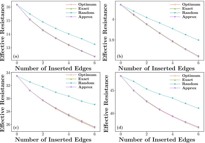
Figure 1. Effective resistance for a set $Q$ of $q=3$ leader nodes as a function of the number $k$ of inserted edges for Exact, Approx, random and the optimum solution on four networks: (a) Karate, (b) Windsufers, (c) Dolphins, and (d) Lesmis.

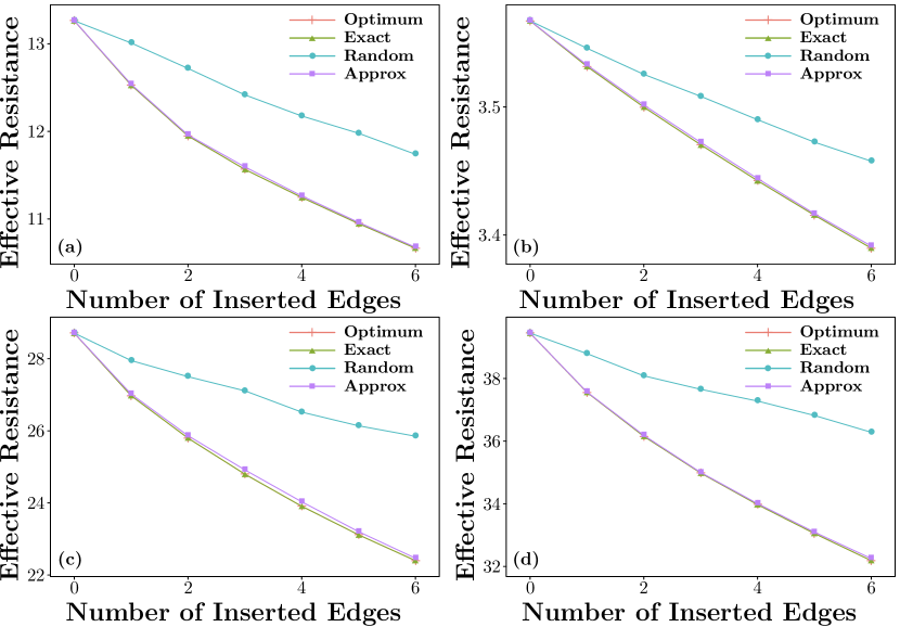
Figure 2. Effective resistance for a set $Q$ of $q=5$ leader nodes as a function of the number $k$ of inserted edges for Exact, Approx, random and the optimum solution on four networks: (a) Karate, (b) Windsufers, (c) Dolphins, and (d) Lesmis.

To further show the accuracy of our algorithms, we continue to compare our algorithms with some schemes on four larger networks, including Chicago, Hamster Full, Facebook, and HepTh. Since these networks are large, we can hardly obtain the optimum solutions. We consider the following three baselines, random scheme, TopDegree, and TopCent. In TopDegree (TopCent) scheme, we choose the node in $V\setminus Q$ with the highest degree (smallest effective resistance) and link it to random $k$ nodes in $Q$. We also consider two cases: $|Q|=5$ and $|Q|=10$. In Figures 3 and 4, we report the results for $k=1,2,\ldots,20$. Both figures show that there is little difference between the solutions of our two greedy algorithms, which are significantly better than the solutions of the three baselines.

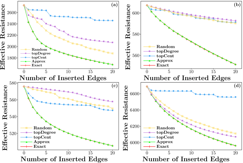
Figure 3. Effective resistance for a set $Q$ of $q=5$ leader nodes as a function of the number $k$ of inserted edges for five heuristics, Exact, Approx, random, TopDegree, and TopCent on four networks: (a) Chicago, (b) Hamster Full, (c) Facebook, and (d) HepTh.

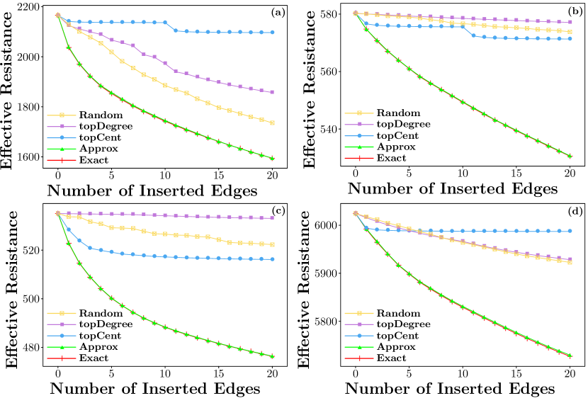
Figure 4. Effective resistance for a set $Q$ of $q=10$ leader nodes as a function of the number $k$ of inserted edges for five heuristics, Exact, Approx, random, TopDegree, and TopCent on four networks: (a) Chicago, (b) Hamster Full, (c) Facebook, and (d) HepTh.

7.2. Efficiency Comparison of Greedy Algorithms

Although both greedy algorithms Approx and Exact produce good solutions, we will show that they differ greatly in the efficiency. For this purpose, we compare the running time of Approx and Exact on some realistic networks. For every network, we randomly select a candidate set $Q$ of 10 target vertices, and calculate the effective resistance of $Q$ after adding $k=20$ new edges incident to vertices in $Q$ and $V\setminus Q$, and record the running time. In Table 1, We list the running time of the two greedy algorithms. It can be observed that for small networks with less than 18,000 nodes, Approx performs a little slowly for most cases. However, for those networks with more than 22,000 nodes, Approx is always much faster than Exact, and gradually becomes faster as the node number increases. Moreover, for those networks with more than 100,000 nodes, Exact fails due to the high time and memory cost, Approx can still solve the effective resistance. Finally, it should be stressed that although Approx is more efficient than Exact, the solutions returned by both algorithms are very close to each other, as shown in Table 2.

Table 2. Effective resistance of a group $Q$ of 10 vertices returned by algorithms Approx and Exact for some real-world networks, as well as the ratios of results of Approx to those of Exact.

Network	Effective Resistance
	Exact	Approx	Ratio
Karate	6.2001	6.2909	1.0147
Windsurfers	2.5033	2.5130	1.0039
Dolphins	14.4097	14.5323	1.0085
Lesmis	20.0719	20.1304	1.0029
Adjnoun	23.0843	23.3235	1.0104
Celegansneural	38.0503	38.1220	1.0019
Chicago	1617.9612	1674.8639	1.0352
Hamster Full	529.1304	529.6522	1.0010
Facebook	487.8539	489.6902	1.0038
GrQc	2992.4740	3034.0660	1.0139
Power Grid	9518.0740	9836.8890	1.0335
High Energy	4883.3000	4931.2573	1.0098
Reactome	1433.9990	1442.4733	1.0059
Route Views	4879.2456	4925.0080	1.0094
HepTh	5660.1680	5694.3535	1.0060
Pretty Good Privacy	14984.6100	15156.1290	1.0114
HepPh	4452.0347	4460.0850	1.0018
AstroPh	4515.5264	4523.1973	1.0017
Internet	16376.9200	16472.5400	1.0058
CAIDA	19731.6020	19940.6800	1.0106
Enron Email	18210.8300	18242.4260	1.0017
Condensed Matter	15298.2550	15329.9380	1.0021
Brightkite	41192.2230	41240.6560	1.0012

8. Conclusions

We examined the problem of minimizing the polarization of the leader-follower opinion dynamics in a noisy social network $G=(V,E)$ with $n$ nodes and $m$ edges, where a group $Q\subset V$ of $q$ nodes are leaders, by adding $k$ new edges incident to the nodes in $Q$. It is a combinatorial optimization problem with an exponential computational complexity, and is equivalent to minimizing the sum of resistance distance $\mathcal{R}_{Q}$ between the node group $Q$ and all other nodes. We proved that the object function is monotone and supermodular. We then presented two approximation algorithms for computing $\mathcal{R}_{Q}$: the former returns a $(1-{1}/{e})$ approximation of the optimum in time $O((n-q)^{3})$, while the latter provides a $\left(1-{1}/{e}-\epsilon\right)$ approximation in time $\widetilde{O}(mk\epsilon^{-2})$. We also compared our algorithms with several potential alternative algorithms. Finally, we performed extensive experiments on real-life networks, which demonstrate our algorithms outperform the baseline methods and can often compute an approximate optimal solution. In particular, our second algorithm can yield a good approximate solution very fast, making it scalable to large-scale networks with more than one million nodes.

References

- (1)
- Abebe et al. (2018) Rediet Abebe, Jon Kleinberg, David Parkes, and Charalampos E Tsourakakis. 2018. Opinion dynamics with varying susceptibility to persuasion. In Proceedings of the 24th ACM SIGKDD International Conference on Knowledge Discovery & Data Mining. ACM, 1089–1098.
- Achlioptas (2003) Dimitris Achlioptas. 2003. Database-friendly random projections: Johnson-Lindenstrauss with binary coins. J. Comput. System Sci. 66, 4 (2003), 671–687.
- Altafini (2013) Claudio Altafini. 2013. Consensus problems on networks with antagonistic interactions. IEEE Trans. Automat. Control 58, 4 (2013), 935–946.
- Amelkin and Singh (2019) Victor Amelkin and Ambuj K Singh. 2019. Fighting opinion control in social networks via link recommendation. In Proceedings of the 25th ACM SIGKDD International Conference on Knowledge Discovery and Data Mining. ACM, 677–685.
- Anderson and Ye (2019) Brian DO Anderson and Mengbin Ye. 2019. Recent advances in the modelling and analysis of opinion dynamics on influence networks. Int. J. Autom. Comput. 16, 2 (2019), 129–149.
- Bamieh et al. (2012) Bassam Bamieh, Mihailo R Jovanovic, Partha Mitra, and Stacy Patterson. 2012. Coherence in large-scale networks: Dimension-dependent limitations of local feedback. IEEE Trans. Automat. Control 57, 9 (2012), 2235–2249.
- Bindel et al. (2011) David Bindel, Jon Kleinberg, and Sigal Oren. 2011. How Bad is Forming Your Own Opinion?. In Proceedings of the 2011 IEEE 52nd Annual Symposium on Foundations of Computer Science. 57–66.
- Bu et al. (2020) Zhan Bu, Hui-Jia Li, Chengcui Zhang, Jie Cao, Aihua Li, and Yong Shi. 2020. Graph K-means based on leader identification, dynamic game, and opinion dynamics. IEEE Trans. Knowl. Data Eng. 32, 7 (2020), 1348–1361.
- Chen et al. (2018) Xi Chen, Jefrey Lijffijt, and Tijl De Bie. 2018. Quantifying and minimizing risk of conflict in social networks. In Proceedings of the 24th ACM SIGKDD International Conference on Knowledge Discovery and Data Mining. ACM, 1197–1205.
- Clark et al. (2014) Andrew Clark, Basel Alomair, Linda Bushnell, and Radha Poovendran. 2014. Minimizing convergence error in multi-agent systems via leader selection: A supermodular optimization approach. IEEE Trans. Automat. Control 59, 6 (2014), 1480–1494.
- Clark and Poovendran (2011) Andrew Clark and Radha Poovendran. 2011. A submodular optimization framework for leader selection in linear multi-agent systems. In Proceedings of the 50th IEEE Conference on Decision and Control and European Control Conference. IEEE, 3614–3621.
- Cohen et al. (2014) Michael B Cohen, Rasmus Kyng, Gary L Miller, Jakub W Pachocki, Richard Peng, Anup B Rao, and Shen Chen Xu. 2014. Solving SDD linear systems in nearly time. In Proceedings of the forty-sixth annual ACM symposium on Theory of computing. ACM, 343–352.
- DeGroot (1974) Morris H DeGroot. 1974. Reaching a consensus. J. Amer. Statist. Assoc. 69, 345 (1974), 118–121.
- Dong et al. (2017) Yucheng Dong, Zhaogang Ding, Luis Martínez, and Francisco Herrera. 2017. Managing consensus based on leadership in opinion dynamics. Inf. Sci. 397 (2017), 187–205.
- Friedkin and Johnsen (1990) Noah E Friedkin and Eugene C Johnsen. 1990. Social influence and opinions. J. Math. Sociol. 15, 3-4 (1990), 193–206.
- Gaitonde et al. (2020) Jason Gaitonde, Jon Kleinberg, and Eva Tardos. 2020. Adversarial perturbations of opinion dynamics in networks. In Proceedings of the 21st ACM Conference on Economics and Computation. 471–472.
- Garimella et al. (2017) Kiran Garimella, Gianmarco De Francisci Morales, Aristides Gionis, and Michael Mathioudakis. 2017. Reducing Controversy by Connecting Opposing Views. In Proceedings of the Tenth ACM International Conference on Web Search and Data Mining. ACM, 81–90.
- Ghosh et al. (2008) Arpita Ghosh, Stephen Boyd, and Amin Saberi. 2008. Minimizing effective resistance of a graph. SIAM Rev. 50, 1 (2008), 37–66.
- Ishakian et al. (2012) Vatche Ishakian, Dóra Erdös, Evimaria Terzi, and Azer Bestavros. 2012. A framework for the evaluation and management of network centrality. In Proceedings of the 2012 SIAM International Conference on Data Mining. 427–438.
- Izmailian et al. (2013) N Sh Izmailian, R Kenna, and FY Wu. 2013. The two-point resistance of a resistor network: a new formulation and application to the cobweb network. J.Phys. A: Math. Theoret. 47, 3 (2013), 035003.
- Johnson and Lindenstrauss (1984) William B Johnson and Joram Lindenstrauss. 1984. Extensions of Lipschitz mappings into a Hilbert space. Contemp. Math. 26 (1984), 189–206.
- Kunegis (2013) Jérôme Kunegis. 2013. Konect: the koblenz network collection. In Proceedings of the 22nd International Conference on World Wide Web. ACM, 1343–1350.
- Kyng and Sachdeva (2016) Rasmus Kyng and Sushant Sachdeva. 2016. Approximate Gaussian elimination for Laplacians-fast, sparse, and simple. In Proceedings of the 57th Annual Symposium on Foundations of Computer Science. IEEE, 573–582.
- Ledford (2020) Heidi Ledford. 2020. How Facebook, Twitter and other data troves are revolutionizing social science. Nature 582, 7812 (2020), 328–330.
- Leskovec and Sosič (2016) Jure Leskovec and Rok Sosič. 2016. SNAP: A general-purpose network analysis and graph-mining library. ACM Trans. Intell. Syst. Technol. 8, 1 (2016), 1.
- Li et al. (2020) Huan Li, Stacy Patterson, Yuhao Yi, and Zhongzhi Zhang. 2020. Maximizing the number of spanning trees in a connected graph. IEEE Trans. Inf. Theory 66, 2 (2020), 1248–1260.
- Li and Schild (2018) Huan Li and Aaron Schild. 2018. Spectral Subspace Sparsification. In Proceedings of 2018 IEEE 59th Annual Symposium on Foundations of Computer Science. IEEE, 385–396.
- Liu et al. (2021) Hui Liu, Xuanhong Xu, Jun-An Lu, Guanrong Chen, and Zhigang Zeng. 2021. Optimizing pinning control of complex dynamical networks based on spectral properties of grounded Laplacian matrices. IEEE Trans. Syst., Man, Cybern., Syst. 51, 2 (2021), 786–796.
- Luca et al. (2014) Vassio Luca, Fagnani Fabio, Frasca Paolo, and Ozdaglar Asuman. 2014. Message Passing Optimization of Harmonic Influence Centrality. IEEE Trans. Control Netw. Syst. 1, 1 (2014), 109–120.
- Ma et al. (2016) Jingying Ma, Yuanshi Zheng, and Long Wang. 2016. Topology selection for multi-agent systems with opposite leaders. Syst. & Control Lett. 93, 7 (2016), 43–49.
- Mackin and Patterson (2019) Erika Mackin and Stacy Patterson. 2019. Maximizing diversity of opinion in social networks. In Proceedings of 2019 American Control Conference. IEEE, 2728–2734.
- Matakos et al. (2017) Antonis Matakos, Evimaria Terzi, and Panayiotis Tsaparas. 2017. Measuring and Moderating Opinion Polarization in Social Networks. Data. Min. Knowl. Disc. 31, 5 (2017), 1480–1505.
- Medya et al. (2018) Sourav Medya, Arlei Silva, Ambuj Singh, Prithwish Basu, and Ananthram Swami. 2018. Group centrality maximization via network design. In Proceedings of the 2018 SIAM International Conference on Data Mining. SIAM, 126–134.
- Meyer (1973) Carl D Meyer, Jr. 1973. Generalized inversion of modified matrices. SIAM J. Appl. Math. 24, 3 (1973), 315–323.
- Musco et al. (2018) Cameron Musco, Christopher Musco, and Charalampos E Tsourakakis. 2018. Minimizing polarization and disagreement in social networks. In Proceedings of the 2018 World Wide Web Conference. 369–378.
- Nemhauser et al. (1978) George L Nemhauser, Laurence A Wolsey, and Marshall L Fisher. 1978. An analysis of approximations for maximizing submodular set functions. Math. Program. 14, 1 (1978), 265–294.
- Noorazar (2020) Hossein Noorazar. 2020. Recent advances in opinion propagation dynamics: a 2020 survey. Eur. Phys. J. Plus 135, 6 (2020), 521.
- Ohara et al. (2017) Kouzou Ohara, Kazumi Saito, Masahiro Kimura, and Hiroshi Motoda. 2017. Maximizing network performance based on group centrality by creating most effective -links. In 2017 IEEE International Conference on Data Science and Advanced Analytics. IEEE, 561–570.
- Parotsidis et al. (2016) Nikos Parotsidis, Evaggelia Pitoura, and Panayiotis Tsaparas. 2016. Centrality-aware link recommendations. In Proceedings of the 9th ACM International Conference on Web Search and Data Mining. ACM, 503–512.