Intermittency in the not-so-smooth elastic turbulence

Abstract

Elastic turbulence is the chaotic fluid motion resulting from elastic instabilities due to the addition of polymers in small concentrations at very small Reynolds (Re) numbers. Our direct numerical simulations show that elastic turbulence, though a low Re phenomenon, has more in common with classical, Newtonian turbulence than previously thought. In particular, we find power-law spectra for kinetic energy $E(k)\sim k^{-4}$, and polymeric energy, $E_{\rm p}(k)\sim k^{-3/2}$, independent of the Deborah (De) number. This is further supported by calculation of scale-by-scale energy budget which shows a balance between the viscous term and the polymeric term in the momentum equation. In real space, as expected, the velocity field is smooth, i.e., the velocity difference across a length scale $r$, $\delta u\sim r$ but, crucially, with a non-trivial sub-leading contribution $r^{3/2}$ which we extract by using the second difference of velocity. The structure functions of second difference of velocity up to order $6$ show clear evidence of intermittency/multifractality. We provide additional evidence in support of this intermittent nature by calculating moments of dissipation rate of kinetic energy averaged over a ball of radius $r$, $\varepsilon_{r}$, from which we calculate the multifractal spectrum.

I Introduction

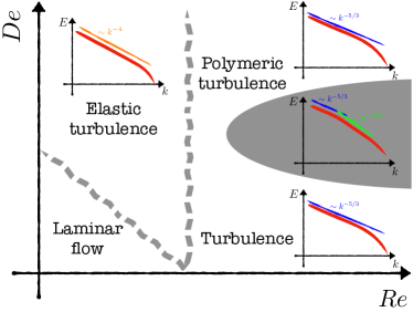
Figure 1: Polymeric flows. An illustrative sketch of the different regimes of polymer-laden flows: classical Newtonian turbulence (HIT) at large Re and zero (or small) De, polymeric turbulence (PHIT) at large Re and De, and elastic turbulence (ET) at small Re and large De.

Turbulence is a state of irregular, chaotic and unpredictable fluid motion at very high Reynolds numbers Re, which is the ratio of typical inertial forces over typical viscous forces in a fluid. It remains one of the last unsolved problems in classical physics. Conceptually, the fundamental problem of turbulence shows up in the simplest setting of statistically stationary, homogeneous and isotropic turbulent (HIT) flows: What are the statistical properties of velocity fluctuations in this ideal set-up? More precisely, consider the (longitudinal) structure function of velocity difference across a length-scale $r$:

$$S_{\rm p}(r) \equiv\left\langle\left[\delta u(\bm{r})\right]^{p}\right\rangle\/,\quad\text{where}$$ (1a)

$$\delta u(r) \equiv\left[u_{\alpha}({\bm{x}}+\bm{r})-u_{\alpha}({\bm{x}})\right]\frac{r_{\alpha}}{\lvert\bm{r}\rvert}\/,$$ (1b)

where ${\bm{u}}({\bm{x}})$ describes the velocity field as a function of the coordinates ${\bm{x}}$ and the symbol $\left\langle\cdot\right\rangle$ denotes averaging over the statistically stationary state of turbulence. The $p$-th order structure function $S_{\rm p}$ is the $p$-th moment of the probability distribution function (PDF) of velocity differences – if we know $S_{\rm p}$ for all $p$ then we know the PDF. Typically, energy is injected into a turbulent flow at a large length scale $L$, while viscous effects are important at small length scales $\eta$, called the Kolmogorov scale, and dissipate away energy from the flow. In the intermediate range of scales $S_{\rm p}(r)\sim r^{\zeta_{\rm p}}$ where scaling exponents $\zeta_{\rm p}$ are universal, i.e. they do not depend on how turbulence is generated. The dimensional arguments of Kolmogorov give $\zeta_{\rm p}=p/3$, which also implies that the shell–integrated energy spectrum (distribution of kinetic energy across wavenumbers) $E(k)\sim k^{-5/3}$, where $k$ is the wavenumber. Experiments and direct numerical simulations (DNS) over last seventy years have now firmly established that the $\zeta_{\rm p}(p)$ is a nonlinear convex function – a phenomenon called multiscaling or intermittency. Even within the Kolmogorov theory, turbulence is non-Gaussian because the odd order structure functions (odd moments of the PDF of velocity differences) are not zero. Intermittency is not merely non-Gaussianity, it implies that not only a few small order moments but moments at all order are important in determining the nature of the PDF. We often write $\zeta_{\rm p}=p/3+\delta_{\rm p}$, where $\delta_{\rm p}$ are corrections due to intermittency. A systematic theory that allows us to calculate $\zeta_{\rm p}$ starting from the Navier–Stokes equation is the goal of turbulence research (Frisch, 1996a).

Turbulent flows, both in nature and industry, are often multiphase, i.e. they are laden with particles, may comprise of fluid mixtures, or contain additives such as polymers. Of these, polymeric flows are probably the most curious and intriguing: the addition of high molecular weight (about $10^{7}$) polymers in $10$–$100$ parts per million (ppm) concentration to a turbulent pipe flow reduces the friction factor (or the drag) upto $5$–$6$ times (depending on concentration) (Toms, 1977; White and Mungal, 2008; Procaccia et al., 2008). Evidently, this phenomena, called turbulent drag reduction (TDR), cannot be studied in homogeneous and isotropic turbulent flows; nevertheless, polymer laden homogeneous and isotropic turbulent (PHIT) flows have been extensively studied theoretically (Bhattacharjee and Thirumalai, 1991; Thirumalai and Bhattacharjee, 1996; Fouxon and Lebedev, 2003a), numerically (Vaithianathan and Collins, 2003; Benzi et al., 2003; Kalelkar et al., 2005; DE ANGELIS et al., 2005; Perlekar et al., 2006; Berti et al., 2006; Peters and Schumacher, 2007; Perlekar et al., 2010; CAI et al., 2010; De Lillo et al., 2012; Watanabe and Gotoh, 2013; Valente et al., 2014; Nguyen et al., 2016a; Valente et al., 2016; Fathali and Khoei, 2019; Rosti et al., 2023), and experimentally (Zhang et al., 2021; Friehe and Schwarz, 1970; McComb et al., 1977; Liberzon et al., 2006; OUELLETTE et al., 2009), to understand how the presence of polymers modifies turbulence, following the pioneering work by Lumley (1973) and Tabor and de Gennes (1986). The simplest way to capture the dynamics of polymers in flows is to model the polymers as two beads connected by an overdamped spring with a characteristic time scale $\tau_{\rm p}$. A straightforward parameterisation of the importance of elastic effects is the Deborah number $\mbox{De}\equiv\tau_{\rm p}/\tau_{\rm f}$, where $\tau_{\rm f}$ is some typical time scale of the flow. In turbulent flows, such a definition becomes ambiguous because turbulent flows do not have a unique time scale, rather we can associate an infinite number of time scales even with a single length scale (L’vov et al., 1997; Mitra and Pandit, 2004; Ray et al., 2011). In such cases, a typical timescale used to define De is the large eddy turnover time of the flow, $\tau_{\rm L}$ (Rosti et al., 2023).

The phenomena of TDR and PHIT appear at high Reynolds and high Deborah numbers. Research in polymeric flows turned into a novel direction when it was realised that even otherwise laminar flows may become unstable due to the instabilities driven by the elasticity of polymers (Larson, 1992; Shaqfeh, 1996). Even more dramatic is the phenomena of elastic turbulence (ET) (Steinberg, 2021), where polymeric flows at low Reynolds but high Deborah numbers are chaotic with mixing, with a shell–integrated kinetic energy spectrum $E(k)\sim k^{-\xi}$. It is still unclear whether this exponent is universal or not – experiments and DNS in two and three dimensions have obtained $3\leq\xi\leq 4$, and theory (Fouxon and Lebedev, 2003b) sets a lower bound with $\xi>3$. In summary, as shown in Fig. (1A), HIT (in Newtonian turbulence) appears at large Re and zero (and small) De; PHIT appears at large Re and large De number (TDR appears in the same region), while ET appears at small Reynolds and large Deborah numbers.

Recently, experiments (Zhang et al., 2021) and DNS (Rosti et al., 2023) revealed an intriguing aspect of PHIT: The energy spectrum showed not one but two scaling ranges, a Kolmogorov-like inertial range at moderate wave numbers and a second scaling range with $E(k)\sim k^{-2.3}$ resulting purely due to the elasticity of polymers (Rosti et al., 2023). Even more surprising is the observation that both of these ranges have intermittency correction $\delta_{\rm p}$ which are the same. This hints that even at low Re, where elastic turbulence (ET) appears, intermittent behavior may exist. In this paper, based on large resolution DNS of polymeric flows at low Reynolds number, we show that this is indeed the case.

II Model

Figure 2: Flow visualizations. Two-dimensional slices of the three-dimensional domain showing snapshots of the normalised (a) fluid dissipation field $\varepsilon_{\rm f}/\left\langle\varepsilon_{\rm f}\right\rangle$ and of (b) the polymer dissipation field $\varepsilon_{\rm p}/\left\langle\varepsilon_{\rm p}\right\rangle$ in ET (for $\mbox{De}=9$).

We generate a statistically stationary, homogeneous, isotropic flow of a dilute polymer solution via the DNS of the Navier-Stokes equations coupled to the evolution of polymers described by the Oldroyd-B model:

$$\rho_{\rm f}\left(\partial_{t}u_{\alpha}+u_{\beta}\partial_{\beta}u_{\beta}\right) =-\partial_{\alpha}p+\partial_{\beta}\left(2\mu_{\rm f}S_{\alpha\beta}+\frac{\mu_{\rm p}}{\tau_{\rm p}}C_{\alpha\beta}\right)+\rho_{\rm f}F_{\alpha},$$ (2a)

$$\partial_{t}C_{\alpha\beta}+u_{\beta}\partial_{\beta}C_{\alpha\beta} =C_{\alpha\gamma}\partial_{\gamma}u_{\beta}+C_{\gamma\beta}\partial_{\alpha}u_{\gamma}-\frac{1}{\tau_{\rm p}}\left(C_{\alpha\beta}-\delta_{\alpha\beta}\right)\/.$$ (2b)

Here, ${\bm{u}}$ is the incompressible solvent velocity field, i.e. $\partial_{\beta}u_{\beta}=0$, $p$ is the pressure, $\mathcal{S}$ is the rate-of-strain tensor with components $S_{\alpha\beta}\equiv(\partial_{\alpha}u_{\beta}+\partial_{\beta}u_{\alpha})/2$, $\mu_{\rm f}$ and $\mu_{\rm p}$ are the fluid and polymer viscosities, $\rho_{\rm f}$ is the density of the solvent fluid, $\tau_{\rm p}$ is the polymer relaxation time, and $\mathcal{C}$ is the polymer conformation tensor whose trace $C_{\gamma\gamma}$ is the total end-to-end squared length of the polymer. To maintain a stationary state, we inject energy into the flow using an Arnold-Beltrami-Childress (ABC) forcing, i.e., $\bm{F}=(\mu_{\rm f}/\rho_{\rm f})[(A\sin z+C\cos y)\,{\bf\hat{x}}+(B\sin x+A\cos z)\,{\bf\hat{y}}+(C\sin y+B\cos x)\,{\bf\hat{z}}]$. The injected energy is ultimately dissipated away by both the Newtonian solvent ($\varepsilon_{\rm f}$) and polymers ($\varepsilon_{\rm p}$):

$$\varepsilon_{\rm T}\equiv \varepsilon_{\rm f}+\varepsilon_{\rm p}\qquad\text{where}$$ (3)

$$\varepsilon_{\rm f}\equiv\frac{2\mu_{\rm f}}{\rho_{\rm f}}\left\langle S_{\alpha\beta}S_{\alpha\beta}\right\rangle\,; \varepsilon_{\rm p}\equiv\frac{\mu_{\rm p}}{2\rho_{\rm f}\tau_{\rm p}^{2}}\left\langle C_{\gamma\gamma}-3\right\rangle,$$ (4)

$\varepsilon_{\rm T}$ being the total rate of energy dissipation. We solve eqns. 2a, 2b on a $L=2\pi$ tri-periodic box discretized by $N^{3}=1024^{3}$ collocation points, such that $L/N=\Delta\approx 0.05\eta$, via a second order central-difference scheme. Integration in time is performed using the second order Adams-Bashforth method with a time stepping $\Delta t\approx 10^{-5}\tau_{\rm K}$.

We choose the value of $\mu_{\rm f}$ to achieve a laminar flow in the Newtonian case with $A=B=C=1$. Next, we set the viscosity ratio $\mu_{\rm f}/(\mu_{\rm f}+\mu_{\rm p})=0.9$ to consider dilute polymer solutions Perlekar et al. (2010), and we vary $\tau_{\rm p}$ over two order of magnitudes. Beyond a certain value of $\tau_{\rm p}$, the flow becomes chaotic, and the resulting flows with $\mbox{De}\gtrsim 1$ are able to sustain elastic turbulence. The energy spectrum of the Newtonian flow (and those for small $\tau_{\rm p}$ ) do not show any power-law range, and drops-off rapidly in wavenumber $k$. We show this spectrum in the supplementary material. The Newtonian ABC flow show Lagrangian chaos in the sense that the trajectories of tracer particles advected by such a flow has sensitive dependence on initial condition (Dombre et al., 1986). Hence we expect that a polymer advected by the flow will go through coil-stretch transition for large enough $\tau_{\rm p}$. The backreaction from such polymers may give rise to elastic turbulence.

We present our results for three different Deborah number flows with $\mbox{De}=1,3,9$ and that have a Taylor scale Reynolds number $\mbox{Re}_{\lambda}\approx 35$. To verify that a turbulent state is sustained by purely elastic effects, we have simulated one of the cases, removing the advective nonlinear term from the momentum equation  (2a), and confirmed the resulting turbulent state.

III Results

Let us begin by looking at the (shell–integrated) fluid energy spectrum

$$E(k)\equiv\int d^{3}{\bm{m}}\left\langle\hat{u}({\bm{m}})\hat{u}(-{\bm{m}})\right\rangle\delta(\lvert{\bm{m}}\rvert-k)\/,$$ (5)

where $\hat{u}({\bm{m}})$ is the Fourier transform of the velocity field ${\bm{u}}({\bm{x}})$. We show the spectra for all three De numbers in Fig. (3a). The spectrum $E(k)$ shows a clear power law-scaling over almost two decades when plotted on a log-log scale. Clearly, $E(k)\sim k^{-\xi}$ with $\xi=4$. We also define energy spectrum associated with polymer degrees of freedom as

$$E_{\rm p}(k)\equiv\left(\frac{\mu_{\rm p}}{\rho_{\rm f}\tau_{\rm p}}\right)\int d^{3}{\bm{m}}\left\langle\hat{B}_{\gamma\beta}({{\bm{m}}})\hat{B}_{\beta\gamma}(-{\bm{m}})\right\rangle\delta(\lvert{\bm{m}}\rvert-k)\/,$$ (6)

where the matrix $\mathcal{B}$ with components $B_{\alpha\gamma}$ is the (unique) positive symmetric square root of the matrix $\mathcal{C}$, i.e., $C_{\alpha\beta}=B_{\alpha\gamma}B_{\gamma\beta}$ Balci et al. (2011); Nguyen et al. (2016b). We show a log-log plot of $E_{\rm p}(k)$ in Fig. (3b) along-with dotted, black lines of slope $-3/2$. We obtain $E_{\rm p}(k)\sim k^{-\chi}$ with $\chi=3/2$. We note that the polymer spectrum scaling range is somewhat smaller than that of $E(k)$. In the statistically stationary state of ET – the effect of the advective nonlinearity must be subdominant – at scales smaller from the scale of external force, the viscous term in the momentum equation must balance the elastic contribution Fouxon and Lebedev (2003b). Using a straightforward scaling argument we obtain : $\xi=2\chi+1$, which is satisfied by the values of $\xi$ and $\chi$ we obtain. For further confirmation we calculate all the contributions to the scale-by-scale kinetic energy budget in Fourier space (see Appendix B for a plot of fluxes). As expected, the contribution from the advective term in  (2a) is negligible. The contribution from the elastic and viscous terms are, repectively

$$\mathcal{T}_{\rm p}(K) =\frac{\mu_{\rm p}}{\rho_{\rm f}\tau_{\rm p}}\int^{K}_{k=0}d\Omega\ k^{2}\ dk\ u_{\alpha}({\bm{k}})k_{\beta}C_{\alpha\beta}(-{\bm{k}}),$$ (7a)

$$\mathcal{D}(K) =\frac{\mu_{\rm f}}{\rho_{\rm f}}\int^{K}_{0}d\Omega\ k^{2}\ dk\ k^{2}u_{\alpha}({\bm{k}})u_{\alpha}(-{\bm{k}}),$$ (7b)

where $k=\lvert{\bm{k}}\rvert$ and $\Omega$ is the solid angle in $k$-space. Earlier theoretical arguments (Fouxon and Lebedev, 2003b) have suggested $\xi>3$ which has also been observed in experiments (Groisman and Steinberg, 2000, 2004; Varshney and Steinberg, 2019) – $\xi\approx 3.5$ over less than a decade of scaling range. We obtain $\xi\approx 4$ which satisfies the inequality and agrees with shell-model simulations (Ray and Vincenzi, 2016). Note further that experiments often obtain power-spectrum as a function of frequency and they can be compared with power-spectrum as a function of wavenumber (typically obtained by DNS) by using the Taylor “frozen-flow” hypothesis (Frisch, 1996b). In the absence of a mean flow and negligible contribution from the advective term it is not a priori obvious that the Taylor hypothesis should apply to ET. We have confirmed from our DNS that a frequency dependent power-spectrum obtained from time-series of velocity at a single Eulerian point also gives $\xi=4$ (see Appendix LABEL:smt:energy). Earlier theoretical arguments (Fouxon and Lebedev, 2003b; Steinberg, 2019) had assumed the same balance in the momentum equation that we have, but in addition had assumed scale separation and a large scale alignment of polymers in analogy with magnetohydrodynamics, obtaining $\xi=\chi+2$, which is not satisfied by our DNS.

Next, we consider the second order structure function, $S_{\rm 2}(r)$, which is the inverse Fourier transform of $E(k)$. A straightforward power counting shows that if $S_{\rm 2}(r)\sim r^{\theta_{\rm 2}}$ then $\theta_{\rm 2}=-1+\xi=3$ (Frisch, 1996a). However, it is well known that for any velocity field whose spectra $E(k)\sim k^{-\xi}$ with $\xi>3$ , $S_{\rm 2}(r)\sim r^{2}$, see e.g., Ref. (Pope, 2000, Appendix G). This is also known from the direct cascade regime of two-dimensional turbulence (with Ekman friction) where $E(k)\sim k^{-\gamma}$ with $\gamma>3$ and $S_{\rm 2}(r)\sim r^{2}$, see e.g., Refs. (Perlekar and Pandit, 2009; Boffetta and Ecke, 2012, page 432). This is confirmed from our simulations as well (see inset of Fig. 3 and Appendix C). Furthermore, we have confirmed that structure functions of even order up to $6$ grow as $r^{p}$ for small $r$, where $p$ is the order. They begin to depart from this analytic scaling at increasingly small $r$ as $p$ increases. Thereby we have checked, following the prescription in Ref. (Schumacher et al., 2007) for HIT, that the structure functions are analytic. The result we obtain by inverse Fourier transform of $E(k)$ is, in fact, a sub-dominant contribution at small $r$. To bring out this sub-dominant contribution, we define the second order structure function of the second difference of velocity (Biferale et al., 2001, 2003):

$$\Sigma_{\rm 2}(r)\equiv\left\langle[u_{\alpha}(x_{\alpha}+r_{\alpha})-2u_{\alpha}(x_{\alpha})+u_{\alpha}(x_{\alpha}-r_{\alpha})]^{2}\right\rangle$$ (8)

where $\alpha$ $(=1,2,3)$ picks up the three cartesian components. We plot $\Sigma_{\rm 2}(r)$ in Fig. (3c); clearly $\Sigma_{\rm 2}(r)\sim r^{\zeta_{\rm 2}}$ with $\zeta_{\rm 2}=3$. This is consistent with the $E(k)$ we obtain from our simulations. In summary, our results imply that in ET the velocity fluctuations can be expanded in an asymptotic series in $r$ as:

$$\left\langle\delta u_{\alpha}({\bm{x}},\bm{r})\right\rangle\equiv\left\langle u_{\alpha}({\bm{x}}+\bm{r})-u_{\alpha}({\bm{x}})\right\rangle\sim G_{\alpha\beta}r_{\beta}+H_{\alpha\beta}r_{\beta}^{h}+\rm{h.o.t}.,$$ (9)

with $h\approx 3/2$. Here, the symbol $\rm{h.o.t}$. denotes higher order terms in $r$. To understand the importance of this result, let us revisit the Kolmogorov theory of turbulence: In the limit $r\to 0$ at a finite viscosity $\mu_{\rm f}$, $\delta u_{\alpha}({\bm{x}},\bm{r})\sim r$ since velocity gradients are finite. But if we first take the limit $\nu\to 0$ and then $r\to 0$ – $\nu\equiv\mu_{\rm f}/\rho_{\rm f}$ is the kinematic viscosity – $\delta u_{\alpha}({\bm{x}},\bm{r})\sim r^{h}$ with $h\approx 1/3$. The velocity field is rough. In contrast, ET is, by definition, a phenomenon at a finite viscosity (small Reynolds number), thus, the limit $\nu\to 0$ does not make sense – the velocity field is always smooth. But the non-trivial nature of ET manifests itself in the first subleading term in the expansion  (9), and this is brought out not by the velocity differences, but by the second difference of velocity across a length scale. This is the first important result of our work.

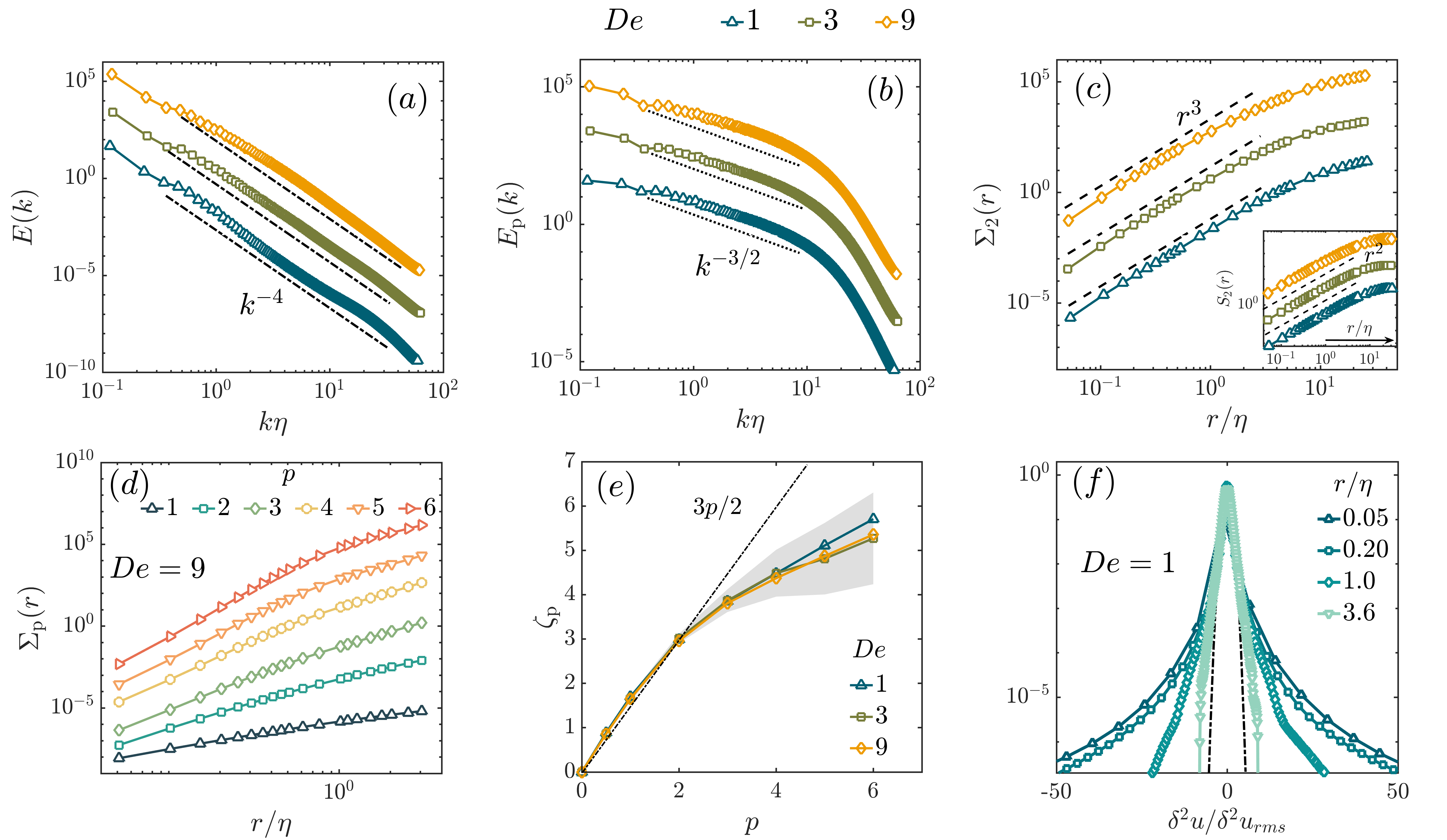
Figure 3: Spectra and structure functions. (a) The fluid energy spectra show a universal scaling $E(k)\sim k^{-4}$ independent of De. A steeper than $k^{-3}$ fall-off of spectrum means the velocity fields are smooth; $S_{\rm 2}(r)\sim r^{2}$ for small $r$, shown in the inset of panel (c). (b) The polymer spectra $E_{\rm p}(k)\sim k^{-3/2}$ follows from the scaling of $E(k)$. (c) Plot of the second order structure function of second differences which scale as $\Sigma_{\rm 2}(r)\sim r^{3}$. The exponent is same for the different De, although the range of scaling depends mildly on De. The inset shows the analytic scaling of second order structure function of first differences of velocity, which clearly indicates that velocity fields are smooth. (d) Second difference structure functions $\Sigma_{\rm p}$, shown for various orders $p$ for $\mbox{De}=9$. (e) The exponents $\zeta_{\rm p}$ versus $p$, calculated from the scaling behaviour of $\Sigma_{\rm p}$. Departure from the straight line $\zeta_{\rm p}=3p/2$ shows intermittency. Shaded region shows the error bars on the exponents. (f) Probability distribution function of $\delta^{\rm 2}u(r)$ for four different values of $r$ at $\mbox{De}=1$. The PDFs for same $r$ but different De falls on top of each other if the abscissa is scaled by the root-mean-square value of the velocity. The distributions are non-Gaussian at small separations, while they become closer to a Gaussian (shown as a black dash-dotted curve) with increasing $r$. The corresponding cumulative distribution functions, computed using the rank-order method, are shown in the Appendix D.

III.1 Intermittency based on velocity differences

The crucial lesson to learn from the previous section is: to uncover the non-trivial scaling of velocities differences we must use the second differences of velocity rather than the usual first difference. So, to study the possibility of intermittency in ET we must study not the usual velocity differences across a length scale but the second differences of velocity. Other than this difference, the rest of this section follows the standard techniques used to study intermittency/multifractality. We look at scaling of structure functions and probability distribution functions (PDFs) $\delta^{\rm 2}u(r)$.

III.1.1 Structure functions

We define the $p$-th order structure function of the second difference of velocity across a length scale $r$ as:

$$\Sigma_{\rm p}(r) \equiv\left\langle\lvert\delta^{\rm 2}u(\bm{r})\rvert^{p}\right\rangle\quad\text{where}\/,$$ (10a)

$$\delta^{\rm 2}u({\bm{r}}) \equiv\left[u_{\alpha}({\bm{x}}+\bm{r})-2u_{\alpha}({\bm{x}})+u_{\alpha}({\bm{x}}-\bm{r})\right]\frac{r_{\alpha}}{\lvert\bm{r}\rvert}\/.$$ (10b)

We show a representative plot of $\Sigma_{\rm p}$’s for all integer $p=1,...,6$ in Fig. (3d) for $\mbox{De}=9$. Clearly, there exists a scaling regime for $r\lesssim 0.8\eta$ for which scaling exponents $\zeta_{\rm p}$ are extracted by fitting $\Sigma_{\rm p}(r)\sim r^{\zeta_{\rm p}}$. The scaling exponents as a function of $p$, are shown in Fig. (3e) where we have also included half-integer values of $p$. For odd and half-integer values of $p$ we have taken absolute value of the velocity differences in  (10b). To obtain reasonable error bars on $\zeta_{\rm p}$, we have proceeded in the following manner. First find a suitable scaling regime for each order by visual inspection. Next, in these chosen ranges, we find the local slopes of the log-log plot of $\Sigma_{\rm p}$’s vs $r$, to obtain $\zeta_{\rm p}$ as a function of $r$:

$$\zeta_{\rm p}(r)=\frac{\Delta\log\Sigma_{\rm p}(r)}{\Delta\log r}\/.$$ (11)

This process is repeated for multiple time snapshots (two successive snapshots are separated by at least one eddy turnover time) of the velocity field data. The set of exponents thus obtained is used to compute the mean exponent $\zeta_{\rm p}$ and the error bars which signify the standard deviation. We show the plot of $\zeta_{\rm p}$ vs $p$ for the De numbers in Fig. (3e). The shaded region shows the error bars. Clearly, $\zeta_{\rm p}$ is a non-linear function of $p$. This unambiguously establishes the existence of intermittency in ET.

III.1.2 PDF of $\delta^{\rm 2}u$

Another way to demonstrate the effects of intermittency is by looking at the PDF of second differences. From the structure function we have obtained intermittent behavior for scales $r/\eta<1$. Thus, we expect the PDF of velocity differences to be close to Gaussian for $r/\eta\gg 1$ and to have long tails (decaying slower than Gaussians) for $r/\eta<1$. This indeed is the case, as is shown in Fig. (3f) where we plot the PDFs for different separations $r$ (for $\mbox{De}=1$). The tails of the distribution of $\delta^{\rm 2}u$ are, in fact, exponential, which decays much slower than a Gaussian, providing yet another evidence for intermittency in ET (see Appendix D). For Newtonian HIT the kurtosis of these PDFs increases as the scale $r$ decreases, $\mathcal{K}\sim r^{-0.11}$ (Chavarria et al., 1995), another signature of intermittency which becomes stronger at smaller scales. In ET, we obtain $\mathcal{K}\sim r^{-1.5}$, see Appendix D. Furthermore, we obtain $\mathcal{K}\to 3$ as $r\to L$, which shows that the PDFs tend to become Gaussian for large separations. Crucially, we find that the kurtosis is independent of De. This is further evidence in support of universality of multifractality in ET. The skewness, which is also often used to quantify non-Gaussian behaviour, does not show good statistical convergence.

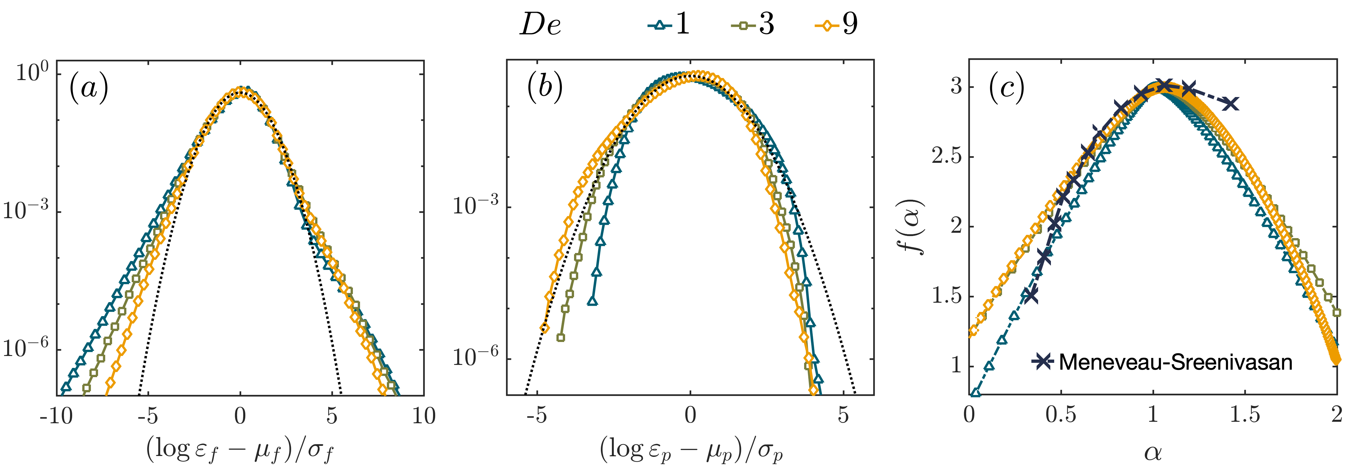
Figure 4: Dissipation rates. (a) PDFs of the logarithm of the fluid energy dissipation rate $\varepsilon_{\rm f}$ for all three De numbers. The distributions deviate significantly from a log-normal behaviour in both the left and right tails. The right tails coincide for large $De$, similar to the coincident right tails at large Re in classical, Newtonian turbulence. (b) PDFs of the logarithm of the polymer energy dissipation rate $\varepsilon_{\rm p}$ for all three De numbers. The PDFs of $\log\varepsilon_{\rm p}$ are sub-Gaussian, i.e. decay faster than a Gaussian, indicating $\varepsilon_{\rm p}$ is not intermittent. (c) The fractal spectra of the fluid dissipation field calculated from the scaling of the energy dissipation rate $\varepsilon_{r}$ calculated over a cube of side $r$. The black dash-dotted line shows the spectrum for classical, Newtonian, HIT taken from Meneveau and Sreenivasan (1991).

III.2 Intermittency based on dissipation

In HIT (high $Re$, Newtonian turbulence) there are two routes to studying intermittency: One is through structure functions and another is through the fluctuations of the energy dissipation rate Frisch (1996b) – the PDF of $\varepsilon_{\rm f}$ deviates strongly from a log-normal behaviour (Andrews et al., 1989). We now take the second route for ET, in which case there are two contributions to the total energy dissipation – $\varepsilon_{\rm f}$ and $\varepsilon_{\rm p}$. In Fig. (4a) and Fig. (4b) we plot the PDFs of the logarithm of $\varepsilon_{\rm f}$ and $\varepsilon_{\rm p}$ respectively. We find that the former decays slower than a Gaussian, i.e., the PDF itself falls off slower than a log-normal, whereas the latter decays faster than a Gaussian. Clearly, the statistics of $\varepsilon_{\rm p}$ are non-intermittent. Henceforth, following the standard analysis pioneered by Meneveau and Sreenivasan (1991) for HIT, we study the scaling of the $q$-th moment of the viscous dissipation averaged over a cube of side $r$,

$$\left\langle\varepsilon_{r}^{q}\right\rangle \sim r^{\lambda_{\rm q}},\quad\text{where}$$ (12a)

$$\varepsilon_{r} \equiv\frac{2\mu_{\rm f}}{\rho_{\rm f}}\left\langle S_{\alpha\beta}S_{\alpha\beta}\right\rangle_{\rm r}\/.$$ (12b)

Here the symbol $\left\langle\cdot\right\rangle_{\rm r}$ denotes averaging over a cube of side $r$. The Legendre transform of the function $\lambda_{\rm q}$ gives the multifractal spectrum (also called the Cramer’s function) $f(\alpha)$:

$$\lambda_{\rm q}=\inf_{\alpha}\left[q(\alpha-1)+3-f(\alpha)\right],$$ (13)

where singularities in the dissipation field with exponent $\alpha-1$ lie on sets of dimension $f(\alpha)$. We plot the $f(\alpha)$ spectrum for ET in Fig. (4c). For comparison, we also plot the multifractal spectrum for HIT as a black dash-dotted curve Meneveau and Sreenivasan (1991). There are minor differences between the multifractal spectrum for $\mbox{De}=3$ and $9$ on one hand and $\mbox{De}=1$ on the other hand. The clear collapse of the multifractal spectra at large De hints towards a universal multifractality in ET in the limit of large De. In HIT the intermittency model based on velocity are closely connected to the intermittency models based on dissipation (Frisch, 1996b). The development of such a formalism for ET, although important, is not considered in this work.

IV Discussion

In summary, we have shown that both the velocity field and the energy dissipation field in ET are intermittent/multifractal. But this multifractality is very different from the multifractality seen in HIT. In HIT, in the limit of viscosity going to zero, the velocity field is rough. In contrast, the velocity field in ET is smooth at leading order, and roughness and the (multi)fractal behavior appears due to the sub-leading term. We have used an unusual definition of structure function, that uses the second difference of velocity, to extract the scaling exponents. Finally, note that in HIT, the multifractal exponents are expected to be universal, i.e., they are independent of the method of stirring and the Reynolds number (in the limit of large Reynolds number). In ET the multifractality appears at small Re and large $\mbox{De}>1$. From Fig. (3e) and Fig. (4c) it may seem that in ET the multifractality has a weak dependence on De. We believe this is not the case, although higher resolution DNSs are necessary to obtain conclusive evidence.

IV.1 Author contributions

M.E.R. and D.M. conceived the original idea. M.E.R. planned and supervised the research, and developed the code. R.K.S. and M.E.R. performed the numerical simulations. R.K.S. analyzed data. R.K.S. and D.M. wrote the first draft of the manuscript. All authors outlined the manuscript content and wrote the manuscript.

IV.2 Competing interests

The authors declare that they have no competing interests.

IV.3 Data availability

All data needed to evaluate the conclusions are present in the paper and/or the Supplementary Materials. Additional data related to this work may be requested from the authors.

IV.4 Code availability

The code used for the present research is a standard direct numerical simulation solver for the Navier–Stokes equations. Full details of the code used for the numerical simulations are provided in the Methods section and references therein.

Appendix A Energy Spectra

We begin by showing the energy spectrum $E(k)$ for the Newtonian and small De (=1/9, 1/3) flows in Fig. (S1a), which remain devoid of any appreciable scaling regime. Energy is concentrated in the largest scales and the energy per mode decays sharply as we go to small scales. In Fig. (S1b), we plot the temporal energy spectrum $E(f)$, for $\mbox{De}=1$, obtained from a simulation on a smaller grid size $N^{3}=512^{3}$. A clear scaling regime of $E(f)\sim f^{-4}$ spans more than a decade in frequencies $f$. This energy spectrum is obtained by applying a Hanning window to the velocity field time-series recorded at a single point, followed by a Fourier transformation and integrating overs different spherical shells of radius $k$ in wave-number space. We also show the independence of our results from the choice of grid resolution in Fig. (S1c) where the plots of fluid energy spectra for $\mbox{De}=1$ from simulations of grid sizes $N^{3}=512^{3}$ (blue) and $N^{3}=1023^{3}$ (yellow) closely follow each-other. The inset shows the spectra from a simulation where the non-linear term was set to zero. This confirms that turbulence-like behaviour is indeed sustained by purely elastic effects.

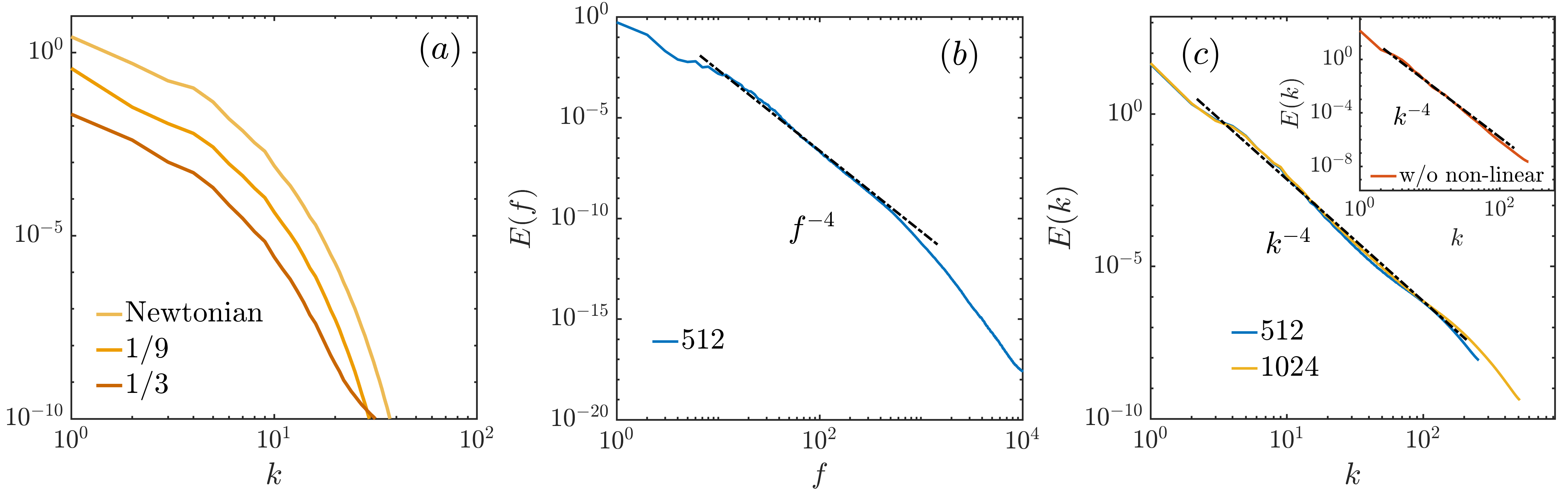
Figure S1: Energy spectra. (a) Energy spectra for Newtonian and small De do not possess any scaling behaviour. The energy per mode falls down sharply to very small values after a decade of waveneumbers. (b) The temporal and (c) spatial energy spectra computed for a smaller grid size $N^{3}=512^{3}$ for $\mbox{De}=1$. The inset shows the spectra obtained from a simulation without the fluid non-linear term.

Appendix B Fluxes

The flux contributions for the fluid dissipation and polymer terms are defined in the main text as:

$$\mathcal{T}_{\rm p}(K) =\frac{\mu_{\rm p}}{\rho_{\rm f}\tau_{\rm p}}\int^{K}_{0}d\Omega\ k^{2}\ dk\ u_{\alpha}({\bm{k}})k_{\beta}C_{\alpha\beta}(-{\bm{k}}),$$ (S1a)

$$\mathcal{D}(K) =\frac{\mu_{\rm f}}{\rho_{\rm f}}\int^{K}_{0}d\Omega\ k^{2}\ dk\ k^{2}u_{\alpha}({\bm{k}})u_{\alpha}(-{\bm{k}}).$$ (S1b)

Similarly, the fluid non-linear flux $\Pi(k)$ can be defined as:

$$\Pi(K)=i\int^{K}_{0}d\Omega\ k^{2}\ dk\ u_{\alpha}(-{\bm{k}})\ \int d{\bm{q}}\ q_{\beta}u_{\beta}({\bm{q}})u_{\alpha}({\bm{k}}-{\bm{q}})$$ (S2)

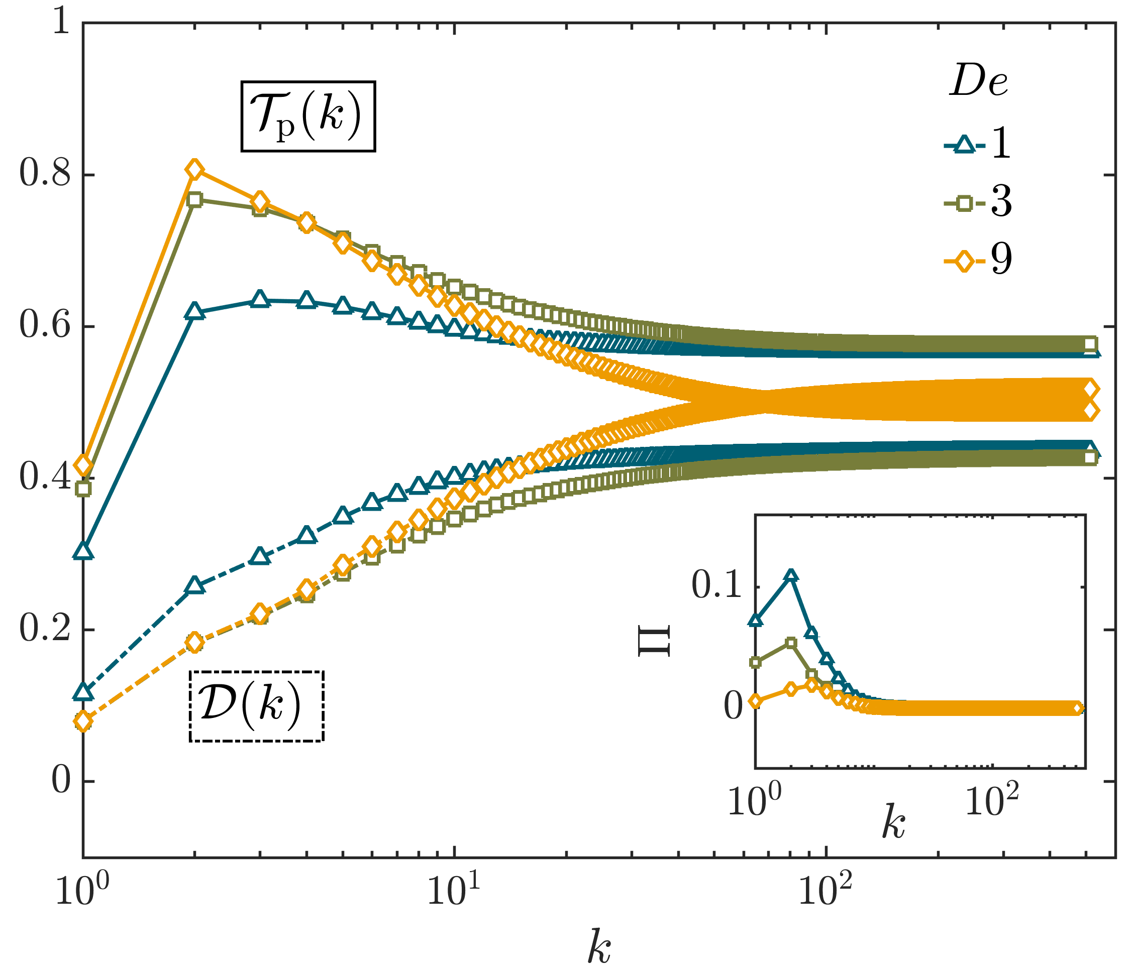
Figure S2: Energy fluxes. The polymeric contribution $\mathcal{T}_{\rm p}(k)$ to the energy transfer to smaller scales compared to the fluid dissipation $\mathcal{D}(k)$ for all three De numbers. The inset shows the near zero contribution of the fluid non-linear flux across scales for $k\geq 10$.

We plot all the flux contributions in Fig. (S2.) The fluid dissipation and polymer contributions are, as expected, comparable over a wide range of scales. It is also clear from the inset that the fluid non-linearity doesn’t play a role in energy transfer to small scales. (The contribution is almost zero for $k\geq 10$ for all De numbers.) This justifies the balance of fluxes argument used to obtain the scaling form of polymer spectrum $E_{p}(k)$ using the expression for $E(k)$.

Appendix C Structure Functions of First Differences

In this section, we plot the usual structure functions defined by the moments of first differences of velocity:

$$S_{\rm p}(r) \equiv\langle\lvert\delta u(\bm{r})\rvert^{p}\rangle\quad\text{where}\/,$$ (S3)

$$\delta u({\bm{r}}) \equiv\left[u_{\alpha}({\bm{x}}+\bm{r})-u_{\alpha}({\bm{x}})\right]\frac{r_{\alpha}}{\lvert\bm{r}\rvert}\/.$$ (S4)

Structure functions $S_{2}$ ($S_{4}$) for different De numbers have been shown in the main (inset) of Fig. (S3a). The structure functions show analytic behaviour for small $r$, the range of which monotonically decreases as one goes up in order $p$. This is seen in Fig. (S3b) where we show the range of analytic scaling by plotting $S_{\rm p}/r^{p}$ for $p=2,4,6$. The initial flat range disappears completely at $p=6$. This is because intermittency effects become important for larger moments, thereby destroying the smooth scaling of velocity fluctuations. The effect of intermittency, however, is independent of polymer elasticity as the analytic range remains unaltered for different De numbers, as seen from Fig. (S3c).

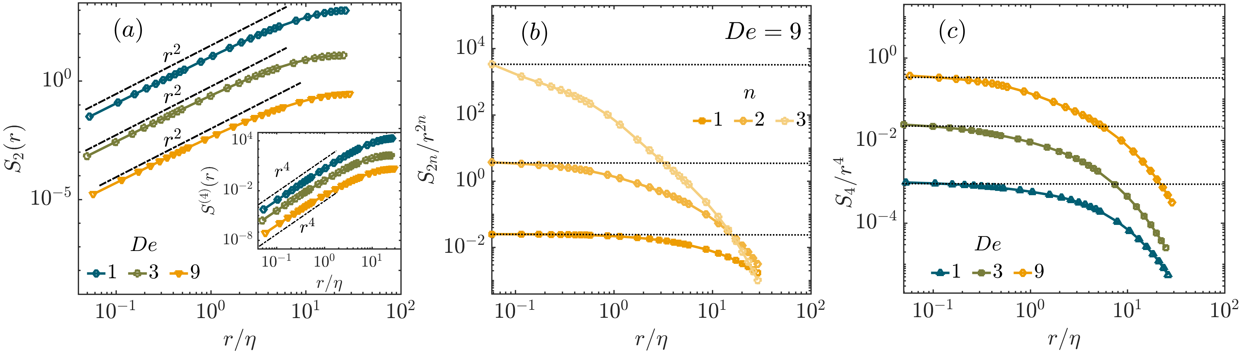
Figure S3: Structure functions. (a) Structure functions $S_{\rm p}(r)$ for $p=2$ shown in the main (inset) panel for $\mbox{De}=1,3$, and $9$. (b) The range of analytic scaling $S_{p}\sim r^{p}$ decreases with increasing order of the moments as intermittent effects become more important. (c) The range of analytic scaling (shown for $S_{4}$) remains independent of De.

Appendix D Cumulative Distribution Functions (CDFs)

We plot in S4 the cumulative distributions of second differences of velocity, where we define the cumulative probability $F(\delta^{2}u)$ as:

$$F(\delta^{2}u)=\left\{\begin{array}[]{lrl}1-\int_{-\infty}^{\infty}p(\delta^{2}u)\;\Theta(\delta^{2}u)\;d(\delta^{2}u),&&\delta^{2}u\geq 0\\ 1-\int_{-\infty}^{\infty}p(\delta^{2}u)\;\Theta(-\delta^{2}u)\;d(\delta^{2}u),&&\delta^{2}u\leq 0\end{array}\right.$$ (S7)

where $\Theta(x)$ is the Heaviside step function and $p(x)$ is the probability distribution function of $x$. The solid lines correspond to the CDFs computed for $\delta^{2}u\geq 0$, while the dashed curves correspond to CDFs for $\delta^{2}u\leq 0$. The CDFs are calculated using rank-order method (Mitra et al., 2005), thereby they are free of binning errors that plague the usual PDFs that are calculated from histogram.

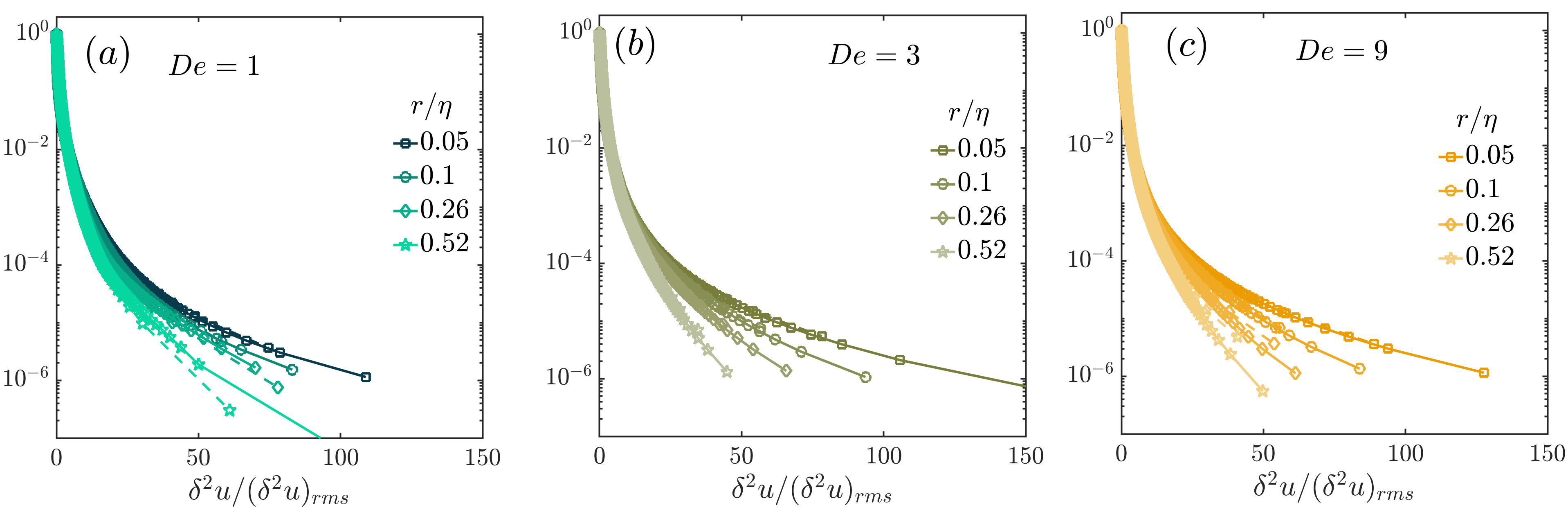
Figure S4: Cumulative Distribution Functions. Normalised (by the root-mean-square) cdfs of the second differences of the $x$-component $\delta^{2}u$ of the velocity field for $\mbox{De}=1$ (a), $3$(b), and $9$(c). The solid and dashed curves correspond to CDFs for $\delta^{2}u\geq 0$ (positive) and $\delta^{2}u\leq 0$ (negative).

We also show the kurtosis of the distributions of velocity second differences, defined as

$$\mathcal{K}(r)=\frac{\langle(\delta^{2}u(r))^{4}\rangle}{\langle(\delta^{2}u(r))^{2}\rangle^{2}}$$ (S8)

in Fig. (S5). For classical, Newtonian, HIT the kurtosis increaes as the scale $r$ decreases as $\mathcal{K}\sim r^{-0.11}$ another signature of intermittency which becomes stronger at smaller scales. In ET, $\mathcal{K}\sim r^{-1.5}$. The fact that $\mathcal{K}\to 3$ as $r\to L$ shows that the PDFs tend to a Gaussian for large separations. Furthermore we find that the kurtosis is independent of De. This is further evidence is support of universality of multifractality in ET. The skewness, which is also often used to quantify non-Gaussian behavior, does not show statistical convergence because it is a sum of quantities with different signs.

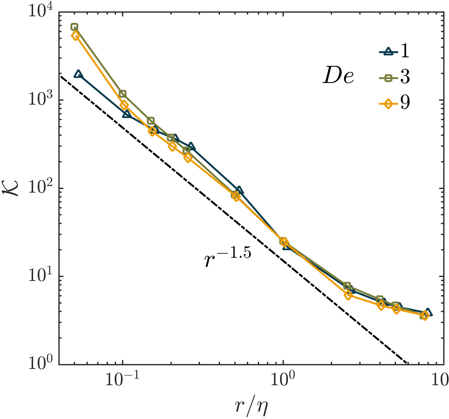
Figure S5: Kurtosis. The kurtosis $\mathcal{K}$ of probability distributions of second differences of one component of $\delta^{2}u$ for $\mbox{De}=1$, $3$ and $9$. The plots of kurtosis for different De lie on top of each other, signalling universality.

References

- Frisch (1996a) U Frisch, Turbulence: The Legacy of A. N. Kolmogorov (Cambridge University Press, 1996).
- Toms (1977) B. A. Toms, “On the early experiments on drag reduction by polymers,” The Physics of Fluids 20, S3–S5 (1977).
- White and Mungal (2008) Christopher M. White and M Godfrey Mungal, “Mechanics and prediction of turbulent drag reduction with polymer additives,” Annual Review of Fluid Mechanics 40, 235–256 (2008).
- Procaccia et al. (2008) Itamar Procaccia, Victor S. L’vov, and Roberto Benzi, “Colloquium: Theory of drag reduction by polymers in wall-bounded turbulence,” Rev. Mod. Phys. 80, 225–247 (2008).
- Bhattacharjee and Thirumalai (1991) J. K. Bhattacharjee and D. Thirumalai, “Drag reduction in turbulent flows by polymers,” Phys. Rev. Lett. 67, 196–199 (1991).
- Thirumalai and Bhattacharjee (1996) D. Thirumalai and J. K. Bhattacharjee, “Polymer-induced drag reduction in turbulent flows,” Phys. Rev. E 53, 546–551 (1996).
- Fouxon and Lebedev (2003a) A. Fouxon and V. Lebedev, “Spectra of turbulence in dilute polymer solutions,” Physics of Fluids 15, 2060–2072 (2003a).
- Vaithianathan and Collins (2003) T. Vaithianathan and Lance R. Collins, “Numerical approach to simulating turbulent flow of a viscoelastic polymer solution,” Journal of Computational Physics 187, 1–21 (2003).
- Benzi et al. (2003) Roberto Benzi, Elisabetta De Angelis, Rama Govindarajan, and Itamar Procaccia, “Shell model for drag reduction with polymer additives in homogeneous turbulence,” Phys. Rev. E 68, 016308 (2003).
- Kalelkar et al. (2005) Chirag Kalelkar, Rama Govindarajan, and Rahul Pandit, “Drag reduction by polymer additives in decaying turbulence,” Phys. Rev. E 72, 017301 (2005).
- DE ANGELIS et al. (2005) E. DE ANGELIS, C. M. CASCIOLA, R. BENZI, and R. PIVA, “Homogeneous isotropic turbulence in dilute polymers,” Journal of Fluid Mechanics 531, 1–10 (2005).
- Perlekar et al. (2006) Prasad Perlekar, Dhrubaditya Mitra, and Rahul Pandit, “Manifestations of drag reduction by polymer additives in decaying, homogeneous, isotropic turbulence,” Phys. Rev. Lett. 97, 264501 (2006).
- Berti et al. (2006) S. Berti, A. Bistagnino, G. Boffetta, A. Celani, and S. Musacchio, “Small-scale statistics of viscoelastic turbulence,” Europhysics Letters 76, 63 (2006).
- Peters and Schumacher (2007) Thomas Peters and Jörg Schumacher, “Two-way coupling of finitely extensible nonlinear elastic dumbbells with a turbulent shear flow,” Physics of Fluids 19, 065109 (2007).
- Perlekar et al. (2010) Prasad Perlekar, Dhrubaditya Mitra, and Rahul Pandit, “Direct numerical simulations of statistically steady, homogeneous, isotropic fluid turbulence with polymer additives,” Phys. Rev. E 82, 066313 (2010).
- CAI et al. (2010) W.-H. CAI, F.-C. LI, and H.-N. ZHANG, “Dns study of decaying homogeneous isotropic turbulence with polymer additives,” Journal of Fluid Mechanics 665, 334–356 (2010).
- De Lillo et al. (2012) F. De Lillo, G. Boffetta, and S. Musacchio, “Control of particle clustering in turbulence by polymer additives,” Phys. Rev. E 85, 036308 (2012).
- Watanabe and Gotoh (2013) Takeshi Watanabe and Toshiyuki Gotoh, “Hybrid eulerian–lagrangian simulations for polymer–turbulence interactions,” Journal of Fluid Mechanics 717, 535–575 (2013).
- Valente et al. (2014) P. C. Valente, C. B. da Silva, and F. T. Pinho, “The effect of viscoelasticity on the turbulent kinetic energy cascade,” Journal of Fluid Mechanics 760, 39–62 (2014).
- Nguyen et al. (2016a) M. Quan Nguyen, Alexandre Delache, Serge Simoëns, Wouter J. T. Bos, and Mamoud El Hajem, “Small scale dynamics of isotropic viscoelastic turbulence,” Phys. Rev. Fluids 1, 083301 (2016a).
- Valente et al. (2016) P. C. Valente, C. B. da Silva, and F. T. Pinho, “Energy spectra in elasto-inertial turbulence,” Physics of Fluids 28, 075108 (2016).
- Fathali and Khoei (2019) Mani Fathali and Saber Khoei, “Spectral energy transfer in a viscoelastic homogeneous isotropic turbulence,” Physics of Fluids 31, 095105 (2019).
- Rosti et al. (2023) Marco E Rosti, Prasad Perlekar, and Dhrubaditya Mitra, “Large is different: non-monotonic behaviour of elastic range scaling in polymeric turbulence at large reynolds and deborah numbers,” Science Advances 9, eadd3831 (2023).
- Zhang et al. (2021) Yi-Bao Zhang, Eberhard Bodenschatz, Haitao Xu, and Heng-Dong Xi, “Experimental observation of the elastic range scaling in turbulent flow with polymer additives,” Science Advances 7, eabd3525 (2021).
- Friehe and Schwarz (1970) Carl A. Friehe and W. H. Schwarz, “Grid-generated turbulence in dilute polymer solutions,” Journal of Fluid Mechanics 44, 173–193 (1970).
- McComb et al. (1977) W. D. McComb, J. Allan, and C. A. Greated, “Effect of polymer additives on the small‐scale structure of grid‐generated turbulence,” The Physics of Fluids 20, 873–879 (1977).
- Liberzon et al. (2006) A. Liberzon, M. Guala, W. Kinzelbach, and A. Tsinober, “On turbulent kinetic energy production and dissipation in dilute polymer solutions,” Physics of Fluids 18, 125101 (2006).
- OUELLETTE et al. (2009) NICHOLAS T. OUELLETTE, HAITAO XU, and EBERHARD BODENSCHATZ, “Bulk turbulence in dilute polymer solutions,” Journal of Fluid Mechanics 629, 375–385 (2009).
- Lumley (1973) J. L. Lumley, “Drag reduction in turbulent flow by polymer additives,” Journal of Polymer Science: Macromolecular Reviews 7, 263–290 (1973).
- Tabor and de Gennes (1986) M. Tabor and P. G. de Gennes, “A cascade theory of drag reduction,” Europhysics Letters 2, 519 (1986).
- L’vov et al. (1997) V.S. L’vov, E. Podivilov, and I. Procaccia, Phys. Rev. E 55, 7030 (1997).
- Mitra and Pandit (2004) D. Mitra and R. Pandit, “Varieties of dynamic multiscaling in fluid turbulence,” Phys. Rev. Lett. 93, 024501 (2004).
- Ray et al. (2011) Samriddhi Sankar Ray, Dhrubaditya Mitra, Prasad Perlekar, and Rahul Pandit, “Dynamic multiscaling in two-dimensional fluid turbulence,” Phys. Rev. Lett. 107, 184503 (2011).
- Larson (1992) R. G. Larson, “Instabilities in viscoelastic flows,” Rheologica Acta 31, 213–263 (1992).
- Shaqfeh (1996) E S G Shaqfeh, “Purely elastic instabilities in viscometric flows,” Annual Review of Fluid Mechanics 28, 129–185 (1996).
- Steinberg (2021) Victor Steinberg, “Elastic turbulence: an experimental view on inertialess random flow,” Annual Review of Fluid Mechanics 53, 27–58 (2021).
- Fouxon and Lebedev (2003b) A. Fouxon and V. Lebedev, “Spectra of turbulence in dilute polymer solutions,” Phys. Fluids. 15, 2060 (2003b).
- Dombre et al. (1986) Thierry Dombre, Uriel Frisch, John M Greene, Michel Hénon, A Mehr, and Andrew M Soward, “Chaotic streamlines in the abc flows,” Journal of Fluid Mechanics 167, 353–391 (1986).
- Balci et al. (2011) Nusret Balci, Becca Thomases, Michael Renardy, and Charles R Doering, “Symmetric factorization of the conformation tensor in viscoelastic fluid models,” Journal of Non-Newtonian Fluid Mechanics 166, 546–553 (2011).
- Nguyen et al. (2016b) M Quan Nguyen, Alexandre Delache, Serge Simoëns, Wouter JT Bos, and Mamoud El Hajem, “Small scale dynamics of isotropic viscoelastic turbulence,” Physical Review Fluids 1, 083301 (2016b).
- Groisman and Steinberg (2000) Alexander Groisman and Victor Steinberg, “Elastic turbulence in a polymer solution,” Nature 405, 53 (2000).
- Groisman and Steinberg (2004) Alexander Groisman and Victor Steinberg, “Elastic turbulence in curvilinear flows of polymer solutions,” New J. Phys. 6 (2004).
- Varshney and Steinberg (2019) Atul Varshney and Victor Steinberg, “Elastic alfven waves in elastic turbulence,” Nature communications 10, 1–7 (2019).
- Ray and Vincenzi (2016) Samriddhi Sankar Ray and Dario Vincenzi, “Elastic turbulence in a shell model of polymer solution,” Europhysics Letters 114, 44001 (2016).
- Frisch (1996b) U. Frisch, Turbulence the legacy of A.N. Kolmogorov (Cambridge University Press, Cambridge, 1996).
- Steinberg (2019) Victor Steinberg, “Scaling relations in elastic turbulence,” Physical review letters 123, 234501 (2019).
- Pope (2000) S.B. Pope, Turbulence (Cambridge University Press, Cambridge, 2000).
- Perlekar and Pandit (2009) Prasad Perlekar and Rahul Pandit, “Statistically steady turbulence in thin films: direct numerical simulations with ekman friction,” New Journal of Physics 11, 073003 (2009).
- Boffetta and Ecke (2012) Guido Boffetta and Robert E Ecke, “Two-dimensional turbulence,” Annual Review of Fluid Mechanics 44, 427–451 (2012).
- Schumacher et al. (2007) Jörg Schumacher, Katepalli R Sreenivasan, and Victor Yakhot, “Asymptotic exponents from low-reynolds-number flows,” New Journal of Physics 9, 89 (2007).
- Biferale et al. (2001) L. Biferale, M. Cencini, A. Lanotte, D. Vergni, and A. Vulpiani, “Inverse statistics of smooth signals: The case of two dimensional turbulence,” Phys. Rev. Lett. 87, 124501 (2001).
- Biferale et al. (2003) Luca Biferale, Massimo Cencini, Alesandra S Lanotte, and Davide Vergni, “Inverse velocity statistics in two-dimensional turbulence,” Physics of Fluids 15, 1012–1020 (2003).
- Chavarria et al. (1995) G. Ruiz Chavarria, C Baudet, and S Ciliberto, “Extended self-similarity of passive scalars in fully developed turbulence,” Europhysics Letters (EPL) 32, 319–324 (1995).
- Meneveau and Sreenivasan (1991) Charles Meneveau and KR Sreenivasan, “The multifractal nature of turbulent energy dissipation,” Journal of Fluid Mechanics 224, 429–484 (1991).
- Andrews et al. (1989) L. C. Andrews, R. L. Phillips, B. K. Shivamoggi, J. K. Beck, and M. L. Joshi, “A statistical theory for the distribution of energy dissipation in intermittent turbulence,” Physics of Fluids A: Fluid Dynamics 1, 999–1006 (1989).
- Mitra et al. (2005) Dhrubaditya Mitra, Jérémie Bec, Rahul Pandit, and Uriel Frisch, “Is multiscaling an artifact in the stochastically forced burgers equation?” Physical review letters 94, 194501 (2005).
Acknowledgements.
The research was supported by the Okinawa Institute of Science and Technology Graduate University (OIST) with subsidy funding from the Cabinet Office, Government of Japan. The authors acknowledge the computer time provided by the Scientific Computing section of Research Support Division at OIST and the computational resources of the supercomputer Fugaku provided by RIKEN through the HPCI System Research Project (Project IDs: hp210229 and hp210269). The authors RKS and MER thank Prof. Guido Boffetta for crucial insights and suggestions and for bringing to our notice Ref. (Biferale et al., 2001). PP acknowledges support from the Department of Atomic Energy (DAE), India under Project Identification No. RTI 4007, and DST (India) Project No. MTR/2022/000867. DM acknowledges the support of the Swedish Research Council Grant No. 638-2013-9243. NORDITA is grudgingly partially supported by NordForsk. DM gratefully acknowledges hospitality by OIST.IV.1 Author contributions