Hybrid Emission Modeling of GRB 221009A: Shedding Light on TeV Emission Origins in Long-GRBs
Abstract
Observations of long duration gamma-ray bursts (GRBs) with TeV emission during their afterglow have been on the rise. Recently, GRB 221009A, the most energetic GRB ever observed, was detected by the LHAASO experiment in the energy band 0.2 - 7 TeV. Here, we interpret its afterglow in the context of a hybrid model in which the TeV spectral component is explained by the proton-synchrotron process while the low energy emission from optical to X-ray is due to synchrotron radiation from electrons. We constrained the model parameters using the observed optical, X-ray and TeV data. By comparing the parameters of this burst and of GRB 190114C, we deduce that the VHE emission at energies 1 TeV in the GRB afterglow requires large explosion kinetic energy, erg and a reasonable circumburst density, cm-3. This results in a small injection fractions of particles accelerated to a power-law, . A significant fraction of shock energy must be allocated to a near equipartition magnetic field, , while electrons should only carry a small fraction of this energy, . Under these conditions required for a proton synchrotron model, namely , the SSC component is substantially sub-dominant over proton-synchrotron as a source of TeV photons. These results lead us to suggest that proton-synchrotron process is a strong contender for the radiative mechanisms explaining GRB afterglows in the TeV band.
1 Introduction
Gamma Ray Bursts (GRB) are indisputably the universe’s brightest extragalactic transient events. They feature a brief prompt phase emission, mostly observed in the energy extending from a few keVs to a few GeVs. It is then followed by the extended broadband afterglow, detected at all energy bands, from radio to a few hundreds of GeVs and possibly even higher (for reviews see e.g. Piran, 1999; Mészáros, 2006; Kumar & Zhang, 2015; Zhang, 2018). Detections of GRB afterglows at the highest energies (i.e., GeV) have been on the rise in the past two decades (for reviews, see, e.g., Nava, 2018; Miceli & Nava, 2022). Understanding the physics underlying this emission has become of highest importance as it holds the clues to better constrain and understand the afterglow of GRBs.
The recent development of highly sensitive ground-based detectors, such as the High Energy Stereoscopic System (H.E.S.S, Aharonian et al., 1997; H. E. S. S. Collaboration et al., 2021), the Major Atmospheric Gamma Imaging Cherenkov (MAGIC, Lorenz, 2005), and the more recent Large High Altitude Air Shower Observatory (LHAASO, Cao et al., 2019), has allowed for the detection of sub-TeV to TeV signal in GRBs and measurements of their spectra in this band. Examples include GRB 180720B (Abdalla et al., 2019), GRB 190114C (Acciari et al., 2019a), GRB 190829A (H. E. S. S. Collaboration et al., 2021) and GRB 201216C (Blanch et al., 2020).
The emission mechanism of GRBs with emission at the very high energy (VHE, TeV) band is highly debated. With reference to the fireball scenario, the synchrotron self-Compton (SSC) model is prominent among the radiation mechanisms that aim to explain these signals. In this mechanism, photons emitted by the synchrotron process at low energies, are upscattered to VHE by the energetic electrons that emitted them (Ghisellini & Celotti, 1998; Dermer et al., 2000; Sari & Esin, 2001; Fraija et al., 2019; Wang et al., 2019; Derishev & Piran, 2021a; Fraija et al., 2022; Yamasaki & Piran, 2022). Alternatively, the proton-synchrotron mechanism has been suggested to produce a photon signal at these extreme energies (Vietri, 1997; Böttcher & Dermer, 1998; Isravel et al., 2022; Zhang et al., 2022). The idea is that the same mechanism responsible for accelerating electrons also accelerates protons to high energies. The energetic protons then emit the observed VHE photons, reaching energies as high as TeV (Totani, 1998; Zhang & Mészáros, 2001; Isravel et al., 2022). In addition, photo-pion and photo-pair production processes may also produce VHE photons (see e.g. Razzaque et al., 2010) although this requires a compact region, and it is not clear how this is obtained at late times.
The recent detection of TeV photons from GRB 221009A allows for the first time to probe in great details the GRB afterglow phase in this energy band. This GRB is by far the brightest GRB ever detected (Lesage et al., 2023). It was observed at the energy band 0.2 - 7 TeV by LHAASO (LHAASO-Collaboration et al., 2023). The isotropic equivalent luminosity in the band TeV is erg s-1 and the observed peak flux is erg cm-2 s-1 (LHAASO-Collaboration et al., 2023). This GRB is a nearby burst, at a cosmological redshift (de Ugarte Postigo A. et al., 2022; Castro-Tirado et al., 2022) as well as the brightest burst ever detected, with an isotropic equivalent burst energy erg (Frederiks et al., 2022). The half opening angle of the jet is estimated to be (LHAASO-Collaboration et al., 2023).
Several authors considered the conventional SSC model to interpret the VHE afterglow spectrum of GRB 221009A. This process is a natural outcome of the classical synchrotron-SSC emission model, and can account for emission in this energy band. However, it is not clear yet whether this model can explain the broad-band data (at all wavelengths), given the strong constraints on the TeV band flux from radio, optical and X-ray data (González et al., 2022; Miceli & Nava, 2022). Furthermore, this model cannot explain a 10 TeV energy photons (Huang. Y., 2022) originally claimed to be observed (González et al., 2022; Ren et al., 2022; Kann et al., 2023; Das & Razzaque, 2023; Laskar et al., 2023a). On the other hand, it is not clear if photons at these energies were detected 111In their analysis, the LHAASO collaboration cut the spectrum at 7 TeV. and required to explain the observed spectra (LHAASO-Collaboration et al., 2023). A recent work by Zhang et al. (2022) considered the possibility that proton-synchrotron may be the source of TeV energy photons in the reverse shock scenario, and concluded that this is a plausible scenario under certain conditions, in particular a very strong magnetic field.
Here, we use the data available from optical through X-rays to TeV, and show that the synchrotron emission from relativistic protons can explain both the flux and the temporal features of the VHE afterglow of GRB 221009A, while its lower-energy afterglow counterpart is interpreted with the electron-synchrotron process. We determined two sets of parameters able to explain the observational features of this burst. Then by comparing these model parameters with those deduced for GRB 190114C (Isravel et al., 2022), we identify a set of consistent characteristics for the VHE afterglows with energies TeV, within the framework of the hybrid model we present.
This paper is structured as follows. In section 2 we review the available data on GRB 221009A obtained by various space-based and ground-based facilities. In section 3, we present our model within the context of the standard fireball scenario. We then use the data to constrain the values of the free physical parameters in section 4. The SEDs are then produced for three different cases in section 5. We investigate the common features encountered in the VHE afterglows of GRBs in section 6. Finally, our conclusions follow in section 7.
2 Observational Data of GRB 221009A
The long-duration GRB 221009A triggered the Gamma-Ray Burst Monitor (GBM) on board the Fermi spacecraft on October 9, 2022, at UT 13:16:59 (Veres et al., 2022). Initially, the GBM captured two separate emission episodes (Lesage et al., 2022). The first occurred between -0 and +43.4 s with a reported peak energy of keV and a fluence of erg cm-2 in the energy range 10-1000 keV. The second episode, being the brightest, exhibited numerous peaks during the time interval +175 to +1458 s. Due to the saturation of the detectors caused by the accumulation of photons in several of these peaks, the exact flux can hardly be measured. Yet, the KONUS-WIND collaboration recently reported the fluence within the energy band 20 keV - 10 MeV (Frederiks et al., 2023).
The High Energy (HE) X-ray telescope on board the Insight-Hard X-ray Modulation Telescope (Insight-HXMT) also triggered and monitored this burst on 9th October 2022, at 13:17:00.050 UT (Tan et al., 2022). This instrument’s primary goal is to observe GRBs and electromagnetic counterparts of gravitational waves (Cai et al., 2021). The Insight-HXMT together with the Gravitational Wave High-energy Electromagnetic Counterpart All-sky Monitor (GECAM-C) measured the emission in the energy band 10 KeV to 6 MeV starting from the precursor of the event until the early afterglow phase for a duration of about 1800 s (An et al., 2023). It was determined that the burst has a total isotropic energy of ergs.
The Fermi-Large Area Telescope (LAT) subsequently observed this GRB between 200 and 800 s following the GBM trigger (Pillera et al., 2022). It is the brightest GRB ever detected by LAT, with a maximum reported photon energy of 99.3 GeV, observed 240 s after . Due to the extreme brightness, the Fermi--LAT detector was saturated during the time period 200-400 s (corresponding to ”bad” time intervals, where the exact flux could not be measured due to the saturation; see Omodei. N., 2022a, b). The LAT data in the energy band 0.1 -1 GeV between 400 s and 800 s was modeled by a power-law spectrum resulting in a spectral index and in a photon flux of ph cm-2 s-1(Pillera et al., 2022).
Nearly 53.3 minutes after the GBM trigger, at UT 14:10:17, the Swift-Burst Alert Telescope (BAT) also triggered and observed GRB 221009A in the hard X-ray band (Dichiara et al., 2022). Starting 143 s after the BAT trigger, Swift-XRT slewed and monitored the then steadily declining X-ray light curve with a photon index and a temporal index of (Evans et al., 2007, 2009).
The optical afterglow in the R-band was measured at 18:45 UT, 4.6 hours after the BAT trigger, corresponding to 5.5 hours after the GBM trigger, with magnitude 16.57 0.02 by the Observatiorio Sierra Nevada (OSN) in Spain (Hu et al., 2022). Considering the strong galactic extinction in the R-band, the AB magnitude is estimated to be 3.710 (Schlegel et al., 1998). The optical and infrared data between 0.2 and 0.5 days are presented in O’Connor et al. (2023) and Gill & Granot (2023), and are corrected for the galactic extinction of 1.32 mag. For instance, 179 s after the BAT trigger, swift-UVOT observed GRB 221009A and recorded a magnitude of 16.68 0.03 in the white filter (Kuin et al., 2022).
Finally, LHAASO’s Water Cheronkov Detector Array (WCDA) (Cao et al., 2019) observed GRB 221009A within its field of view at the time of the GBM trigger. Within a span of 3000 s from the burst trigger, more than 60,000 photons in the energy band 0.2 7 TeV were detected by the LHAASO (LHAASO-Collaboration et al., 2023). Around the phase of the main burst, LHAASO recorded the flux of erg cm-2 s-1 at 1 TeV at the time period between , after correcting for extra-galactic background light (EBL) attenuation222As the VHE photons traversing through cosmological sources experience pair-production by interacting with the EBL, which substantially attenuates the intrinsic spectrum of the source (Ackermann et al., 2012)..
The LHAASO collaboration and the Fermi-GBM collaboration deduced different times for the onset of the afterglow. Lesage et al. (2023) for the Fermi-GBM collaboration argued that the beginning of the afterglow phase was s after the trigger. This is based on the inability of a single decay function to explain the lightcurve at earlier times. On the other hand, interpretation of the LHAASO data in the framework of the external shock, based on the temporal decay of the light-curve lead to estimating the onset of the afterglow at this band already at 226 s after the GBM trigger (LHAASO-Collaboration et al., 2023). The origin of this discrepancy can be due to the superposition of both prompt signal (which should originate from a small radius) and afterglow signal (originating from a forward shock propagating ahead of the jet, at larger radius) in the observations around few hundreds seconds. Therefore, here we will model the LHAASO emission as part of the afterglow and will not attempt to model the GBM data, which, as we will show below, is much brighter than the predicted GBM flux within the framework of our model (assumed to be produced by electron-synchrotron in this energy band).
3 Model Description
In this section, we detail the afterglow dynamics and the emission mechanisms, which serve as the basis of our model attempting to explain the VHE observation of GRB 221009A. We set our analysis within the framework of the fireball evolution scenario (Paczynski, 1990; Piran et al., 1993; Mészáros et al., 1998), further assuming that the high-energy component (GeV TeV) and the low-energy component (eV MeV) of the observed spectrum are produced by synchrotron radiation from the accelerated protons and electrons, respectively via the external shock acceleration. More details on the processes and the model can be found in Isravel et al. (2022), and we remind here only the key assumptions and equations.
When the relativistic jet originating from the compact GRB progenitor encounters the stationary ambient environment, an outward propagating shock-wave is created (Paczynski & Rhoads, 1993; Medvedev & Loeb, 1999). This shock collects and accelerates the ambient matter (both protons and electrons) and generates in-situ a magnetic field. The accelerated particles then produce the observed multi-wavelength emission (see e.g. Sari & Piran, 1995; Sari et al., 1998; Panaitescu & Kumar, 2000). During the afterglow phase, the emission occurs while the outflow expands in a self-similar way, following the Blandford & McKee (1976) solution. We assume here that the ultra-relativistic expansion can be considered adiabatic, i.e. that the radiative losses of the plasma behind the shock are negligible. This is a good approximation for our scenario as accelerated protons should carry most of the internal energy while they do not radiate efficiently.
Under those assumptions, the Lorentz factor of the jet, at a given observed time , is determined only by the isotropic-equivalent explosion kinetic energy , and the ambient ISM density :
| (1) |
where is the speed of light, is the mass of the proton and we took the redshift to be relevant for GRB 221009A. Here and below, in cgs units is employed. Using , one can express the location of the blast wave as a function of the observed time,
| (2) |
Finally, we define the comoving shock expansion (dynamical) time as s.
In order to estimate the observed spectrum, we need to specify the magnetic field and the particle distribution functions. For the former, we take the standard assumption that an (uncertain) fraction, , of the post-shock thermal energy is used in generating a magnetic field. This gives
| (3) |
For the radiating particles, namely protons and electrons, we assume that a fraction of all the particle is injected in the radiative zone with a power-law distribution between some minimum Lorentz factor and maximum Lorentz factor, , such that they carry a fraction of the available internal energy. The power-law index is referred to as . Here, the subscript refers either to electrons or to protons . Energetic consideration provides the constraint .
The minimum Lorentz factors of the protons and electrons are readily obtained as
| (4) | ||||
| (5) |
where is a function of and is equal to for and for (Sari et al., 1998).
Another characteristic particle Lorentz factor is obtained by equating the synchrotron cooling time to the dynamical time, providing the cooling Lorentz factor of the particle. The synchrotron cooling time is given by , where is the Thomson cross-section and . This gives , resulting in
| (6) | ||||
| (7) |
A proton synchrotron model requires the magnetic field to be large, and therefore, from Equations (5) and (6), it follows that , hence the electrons are in the fast cooling regime, and the electron distribution function is a broken power-law with index of 2 between and , and above . However from Equation (4), it is seen that , meaning that the proton population is in the slow cooling regime.
The maximum Lorentz factor of the accelerated particles is obtained by equating the acceleration time to the synchrotron cooling time. It comes
| (8) |
where the numerical coefficient prescribes the acceleration efficiency. The maximum Lorentz factor for protons is
| (9) |
Since , the proton distribution function is a single power-law above with an exponential cutoff at the very high energy end of the proton distribution spectrum, producing an exponential cut-off in the resulting photon spectrum. For electrons, is times smaller than , but as the electron-synchrotron flux at such high energies is very small, we omit the discussion on it here.
Each of those characteristic Lorentz factors in the particle distribution functions is associated to a characteristic synchrotron frequency such that . At these frequencies, the observed synchrotron spectrum presents a spectral break. For the electrons, the observed spectrum is for , where is the observed frequency. The proton synchrotron spectrum is shaped as for .
The characteristic frequencies associated with particles at are given by
| (10) | ||||
| (11) |
The cooling frequency for the electrons is
| (12) |
and the maximum frequency for the protons reads
| (13) |
Hence, the shock accelerated protons can emit synchrotron photons at energies as high as 10 TeV above those detected by LHAASO.
The spectral flux is calculated as follows. The maximum power emitted by a single particle via the synchrotron process at the observed peak frequency is . Assuming the total number of radiating particles to be , the peak flux associated with the electron synchrotron process is
| (14) |
where we normalised the luminosity distance to cm, given the proximity of GRB 221009A at redshift (de Ugarte Postigo A. et al., 2022; Castro-Tirado et al., 2022) corresponding to cm (assuming a flat CDM cosmology with = 69.6 km s-1 Mpc-1, , and , Wright, 2006). Since in our scenario the electrons are in the fast cooling regime, analysing the spectrum reveals that , where keV is the low energy threshold of the XRT instrument and eV is the typical frequency of the optical band. The flux at frequencies lower than and greater than is given by
| (15) |
while the flux at frequencies higher than is given by
| (16) |
Similarly, the peak flux associated with the proton-synchrotron process is given by
| (17) |
and the spectrum within the frequency range for the slow-cooling synchrotron process is a power-law
| (18) |
4 Limitations on the model parameters: An Analytical approach
The best fit to the temporal decay of the X-ray flux as observed by the swift-XRT consists of five breaks at times between s to s. The corresponding decay indices at the break times are presented in the XRT catalogue of the burst (Evans et al., 2009). At observed times s, the decay index in the XRT band is identified to be .333https://www.swift.ac.uk/xrt_live_cat/01126853/ At later times, the lightcurve becomes steeper, and may be associated with a jet break. In order to reproduce the temporal decay in the XRT band with (fast cooling regime, as required by the electron synchrotron model), the condition must be satisfied as .444In the slow cooling regime, the requirement on the electrons power law index is even higher with for .
On the other hand, the TeV temporal decay is (LHAASO-Collaboration et al., 2023). This result is challenging for the SSC model, as it seem outside the expected temporal slope for electrons with a power law index of , which is (Sari & Esin, 2001) in the fast cooling regime.555In the slow cooling regime, assuming , the expected temporal decay in the TeV band is , for . We can therefore exploit the proton-synchrotron model, with proton power law index of in the slow cooling regime, as explained above. This is the index needed to explain the LHAASO data. In fact, setting leads to an energy crisis, as the energy budget in the proton-synchrotron component will be very high. Therefore, in presenting our results for GRB 221009A, we will set a proton power law index , but allow for a different value of in interpreting the TeV data. We will keep the constraint in order to satisfy the XRT temporal decay.
4.1 Constraints for a proton-synchrotron model
 |
 |
 |
 |
 |
|
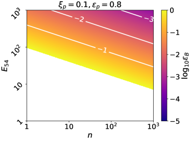
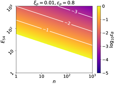
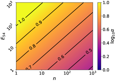
We use the observed flux of GRB 221009A to constrain the values of the free model parameters. We start with the flux at 1 TeV as observed by the LHAASO experiment at time s after the trigger. By equating the LHAASO reported flux ergs cm-2 s-1 (LHAASO-Collaboration et al., 2023) and the expected proton-synchrotron flux given in Equation (18) at 1 TeV, the fractional energy of the magnetic field as a function of the other free parameters is,
which upon setting simplifies to
| (19) |
This value of may seem large, but so should be the kinetic energy of this burst, leading in fact to values of smaller than unity, see the top panel plot on Figure 1.
Similarly, the acceleration efficiency parameter is obtained by comparing from Equation (13) with the observed energy of 7 TeV photon at s,
| (20) |
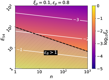
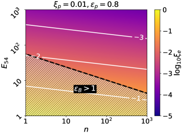
To obtain the values of the other model parameters, we refer to swift-XRT data available at much later times, where XRT data is available and the emission is clearly in the ”afterglow” phase in the swift-XRT band as well. We use Equation (16), which gives the expected energy flux above , together with the observed swift-XRT flux at 3300 s of (at 0.3 keV) and include Equation (4.1) to get the injection fraction of electrons,
Setting and gives
| (21) |
By balancing the swift-UVOT band flux of at observed energy 4.77 eV and observed time s with the predicted synchrotron flux from Equation (15) and including Equations (4.1) and (21), we get
which gives for
| (22) |
This enables to write the parameter as
which simplifies to
| (23) |
for our chosen index values.
The values of , and , as constrained by Equations (4.1), (20) and (23) are plotted in Figure 1 as functions of and for and two choices of , namely (left column) and (right column). Satisfying directly requires that , and should be large while needs to be small. Overall, we could constrain the parameters , , and as functions of the other free model parameters. To provide satisfactory constraints with , the kinetic energy of this burst must be large with . Yet this is not too large compared to the prompt total isotropic energy. In fact, this high kinetic energy would correspond to an efficiency of around 10%, typical of other GRBs (see e.g. Zhang et al., 2007; Beniamini et al., 2016). We note that our goal here is to provide a set of parameters that could potentially explain the TeV observations via the proton synchrotron process and not to determine the best possible parameter values.
We thus find that a requirement of our model is that accelerated protons contribute for most of the internal energy of the shock, with . The magnetic field needs to be strong, , and the circumburst density should be high, . All these require a high kinetic energy. Furthermore, the model requires that only a relatively small fraction of electrons and protons achieve a power-law distribution behind the shock, i.e. and , and that their spectral indices be different, .
4.2 Constraints imposed by the synchrotron-self Compton (SSC) emission.
In the SSC emission mechanism, the electrons that emit the low-energy synchrotron-photons inverse Compton (IC) scatter the same photons to higher energies, thus contributing to the high energy component of the afterglow spectrum. As we derive in details in appendix A, for the parameters chosen, this component is sub-dominant. Here we present the results only for and , but the general trend applies for other values of the injection index . Within the framework of our model, the Klein-Nishina effect for the IC component can be neglected. This is shown by using Equations (1), (5) and (11) at s, to find
| (24) |
This result is in the order of (and even smaller than) , the energy at which the Klein-Nishina effect becomes important. One therefore only expects small modifications, if any, around the peak of the IC component.
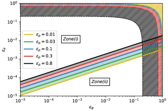
The characteristic frequencies of the IC spectral component for this burst are presented in Appendix A. Equation (A) gives the observed peak energy of the IC spectrum to be around GeV. To determine the criterion that governs the dominance of the proton-synchrotron component over the SSC component, we compare the fluxes at 1 TeV and at 235 s as (Zhang & Mészáros, 2001). We can expand it using Equations (18), (17), (10) and (A) to get the following:
| (25) |
This condition is displayed in Figure 2. The findings depicted in Figure 2 indicate the notion that must exceed in order to satisfy the above condition. Also it is evident that a near equipartition value of reinforces the significant contribution from proton -synchrotron process.
where we assumed that the TeV band is above the frequency of the IC spectral peak, and neglected Klein-Nishina effects. If anything, this effect would further reduce the observed flux in the TeV band, and allow for a larger parameter space in which the proton synchrotron mechanism dominates. This value is orders of magnitude lower than the observed flux at the TeV band, implying that the electron SSC mechanism is sub-dominant at these energies for the constraints we derived.
5 Lightcurve and spectra
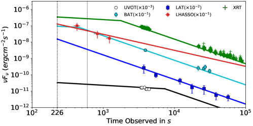
The observed lightcurve of the afterglow of GRB 221009A is shown in Figure 3 alongside the electron and proton synchrotron components estimated from our model. The two different set of parameters used in this section are summarized in Table 1. We set the parameters to , , , and , resulting in , and . The onset of the afterglow phase at 226 s after the burst trigger is marked by the dotted line (LHAASO-Collaboration et al., 2023) whereas the dashed line drawn at t = 597 s marks the end of the prompt duration estimated by Lesage et al. (2023). Overall, this figure demonstrates that the proton synchrotron model presented here is capable of explaining the observed temporal features of the afterglow of GRB 221009A in several different energy bands.
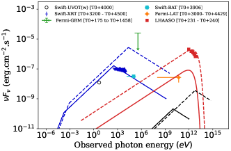
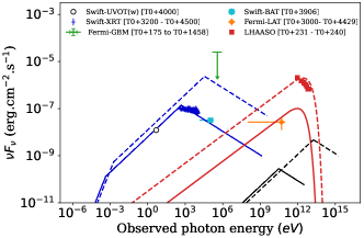
We further produce the afterglow spectrum at two different times, namely at s and s, and display it in Figure 4 (both in the left and right panels). The spectral energy distributions (hereinafter SEDs) consist of three main components. They are produced by the electron-synchrotron, the proton-synchrotron and the IC processes and are respectively shown by the blue, red and black lines. Inspection of Figure 4 (left), obtained for and , shows that the SED of the electron-synchrotron component at 4000 s satisfies the observed data in the optical and X-ray bands as designed in our analytic approach. At the same time, the proton synchrotron component accounts for the LHAASO flux, also marginally satisfies the LAT flux.
We then search for solutions with a smaller proton index, . This is advantageous as it results in a lower burst energy and external density. The right panel of Figure 4 shows the SEDs for the parameters , , , , resulting in , , and . In addition, under this assumption, the required total burst energy is lower than for . Hence the prompt radiative efficiency is increased here. We see that, in this case too, the LAT flux at 4000 s can be marginally explained by the proton synchrotron process.
The close to equipartition values of and associated with all the SEDs are as anticipated for the proton-synchrotron model, see Equations (4.1) and (23). Indeed, protons are more massive than electrons and to radiate a substantial amount of energy, they need a strong magnetic field. We further find that the IC components (black lines in the SEDs shown in Figure 4) are subdominant at all time bins in both scenarios considered, since the magnetic field energy density is large compared to the electron energy density (, see e.g. Rybicki & Lightman, 1986). Indeed, for the constraints we derived, using and , one obtains
The corresponding ratios of the energy densities in our models are given in Table 1.
The lightcurve of the TeV emission is shown to have a break followed by a steeper temporal decay at time s (LHAASO-Collaboration et al., 2023). This break could be obtained by the crossing of the maximum synchrotron frequency through the LHAASO energy band. For the parameters we derived in case and , the time at which equals 1 TeV is . In principle, it is possible to use this property to better constrain the acceleration efficiency, and the other model parameters. However, this constraint depends on the exact parametrization of the proton distribution function at the highest energies, and therefore would bring only little insight into the model, apart from better constraining .
 |
 |
6 Discussion
6.1 Comparison between GRB 221009A and GRB 190114C
Similar to GRB 221009A, GRB 190114C is another long GRB with a VHE afterglow emission observed in the band between 0.2 and 1 TeV (Acciari et al., 2019b). This GRB has an isotropic equivalent energy erg. The redshifts of both GRB 190114C () and GRB 221009A are low, . As a result, the detectability of TeV photons, if produced in the source, is high, since they are only weakly EBL attenuated (see e.g. Franceschini, 2021). Similarly to GRB 221009A, a complete set of multi-wavelength observational data is available for GRB 190114C afterglow (see e.g. MAGIC Collaboration et al., 2019, for a summary of those observations). In Isravel et al. (2022), we considered the proton synchrotron mechanism to explain the VHE afterglow of GRB 190114C.
One can therefore compare the parameters we derived for GRB 221009A to those we obtained for GRB 190114C, in order to outline some of the intriguing features of long GRB associated to VHE energy afterglow observations. Under the guise of a proton synchrotron model, these features are as follows:
6.1.1 Particle index
The parameters associated with yielded the most optimal results in these bursts. One potential cause of protons and electrons having distinct indices is the non-uniformity of the power-law turbulence spectrum of the magnetic field across a wide range of
scales (Asano et al., 2009). This could be realized under several circumstances: a) a difference in scales corresponding to the gyration radii of protons attaining eV, and electrons reaching GeV energies (Cerruti et al., 2015), respectively, and b) a variation in wavelength distribution of shock generated magnetic perturbations and geometry of the magnetic field at the shock front (Niemiec et al., 2006).
On the other hand, the acceleration processes setting these power-law indices in the presence of shock can have varied properties depending upon the orientation of the magnetic field relative to the shock (Caprioli & Spitkovsky, 2014a, b; Guo et al., 2014).
Apart from these, a two-component jet model could also feature different power law indices. In this model, a narrow, highly collimated jet could account for the TeV emission produced by protons, while a less collimated, wider jet could be responsible for the low-energy emission from electrons (Berger et al., 2003; Huang et al., 2004; Sato et al., 2023).
6.1.2 Embedded magnetic field
Requiring that proton synchrotron emission explains the TeV observations results in the necessity of having a strong magnetic field, with close to equipartition. Similarly, the electron equipartition energy must be low, . Even though the inference is inconsistent with the analytical models and particle-in-cell (PIC) simulations of un-magnetized plasma (Medvedev, 2006; Sironi & Spitkovsky, 2011), such a relatively high can be possibly explained as follows.
Considering the connection between long-GRBs and supernovae could account for the highly magnetized environment as well as low (see e.g. Kippen et al., 1998; Bosnjak et al., 2006; Campana et al., 2006; Klose et al., 2019). By performing global fitting of the emission in six supernova remnants (SNRs), Reynolds et al. (2021) found to be between and , while achieves a smaller value in the range of
. These equipartition parameters were determined owing to the advantageous conditions provided by SNRs. This is analogous to the findings in our model for
this GRB and 190114C (Isravel et al., 2022). Also, the compression of the upstream turbulent magnetic field by
the shock may amplifies its strength (Lemoine & Revenu, 2006). The type of turbulence spectrum may also dictate the strength of the magnetic field, such as Kolmogorov turbulence (Biermann & Strittmatter, 1987) and Kraichnan turbulence (Kraichnan, 1965). Alternatively, the reverse shock approximation could also be evoked for proton acceleration as it could harbor such a high magnetization
(Waxman & Bahcall, 2000; Zhang et al., 2018). To explain the VHE emission of GRB 221009A with synchrotron emission from protons accelerated at the reverse shock, Zhang et al. (2022) implemented a strong magnetic field with
.
6.1.3 Injection fraction
The measured fluxes, together with the large kinetic energy, require the fraction of particle accelerated into the power-law to be considerably low,
and .
These values are consistent with the numerical estimation
of considering the acceleration of charged particles in collisionless shocks (Sironi & Spitkovsky, 2011).
A lower than the unity is gaining
attention in the GRB afterglow theories and modeling, see e.g.
Ressler & Laskar (2017); Warren et al. (2018); Cunningham et al. (2020); Asano et al. (2020). For instance, for the very nearby (), GRB 190829A, is obtained by a fit to the data (Salafia et al., 2022).
Also, Gill & Granot (2023) concluded their investigation of GRB 221009A by emphasizing the small value of required by their analysis.
Such a low injection fraction of electrons and protons indicate that there is a large population of thermal particle species present in the
downstream of the shock (Ressler & Laskar, 2017). The thermal particles can indeed be anticipated to emit synchrotron radiation in radio frequencies during the early phase according to Eichler & Waxman (2005).
However, the contribution of these thermal electrons and protons in producing the GRB spectra is yet to be studied in detail (Warren et al., 2018).
6.1.4 Progenitor environment
The progenitor of long-GRBs is a massive star which collapses to form a compact
object (see e.g. Kumar & Zhang, 2015). The low-metallicity Wolf-Rayet stars () with low mass-loss rates () are believed to be progenitors for the collapsar model for which the circumburst density is cm-3 (Woosley et al., 2002; Fryer et al., 2006). Considering in our model, the external medium density of these long duration bursts ranges between cm-3 . When , for a constant ISM medium, the circumburst density estimated in theoretical models is around cm-3 (Beniamini et al., 2015; Gompertz et al., 2018; Derishev & Piran, 2021b; Guarini et al., 2023), and can even reach cm-3 (Laskar et al., 2015) in some specific cases.
6.1.5 Energetics of GRBs
For those two bursts, the required kinetic energy
is larger by about an order of
magnitude than their prompt-phase equivalent energy
. This leads to a radiative efficiency
in the order of 10%. For the proton synchrotron model, we estimated to be about for GRB 190114C and 9% for GRB 221009A considering and for the latter. Moreover, if the jet observed in GRB 221009A is considerably narrow with a half-opening angle of as reported by LHAASO-Collaboration et al. (2023), then the jet kinetic energy after correcting for beaming is erg for and while for and it is erg. This is in agreement with the expectations of amount of energy stored in GRBs (Frail et al., 2001). This analysis is based on the Konus-Wind estimation of erg (Frederiks et al., 2022). However, Insight-HXMT in conjunction with the GECAM-C measured the isotropic equivalent energy of GRB 221009A to be erg (An et al., 2023). The latter measurement is five times higher than the former. It is worthy to highlight that integrating erg into our model leads to an increase in which is around for and and considering and , while the other parameters remain unchanged. We emphasize that both estimates of values yield reasonable prompt phase-energy conversion efficiencies.
6.1.6 Acceleration Efficiency
Finally, we found that these bursts do not require a very efficient proton acceleration, with an efficiency in the order of a few tens, . Interestingly, the PIC simulations performed in Asano et al. (2020) in the context of the VHE afterglow emission of GRB 190114C resulted in even lower efficiency, . It is obtained by considering the early diffusive process in Fermi acceleration mechanism. The parameter in the range acquired by setting the maximum proton energy may imply that high energy protons could be accelerated via MHD turbulence (Demidem et al., 2018; Asano et al., 2020).
6.2 Comparison of SSC and proton-synchrotron components for GRB 221009A
Many authors attempt to explain the VHE observations of GRB afterglow with a purely leptonic modeling based on the synchrotron self-Compton process (for instance Zhang et al., 2022; González et al., 2022; Ren et al., 2022; Laskar et al., 2023a; Kann et al., 2023; Das & Razzaque, 2023; LHAASO-Collaboration et al., 2023). It is argued that explaining the high energy photon with this mechanism is difficult because the modelled SSC flux in the TeV band, which is strongly constrained by the radio, optical and X-ray fluxes, is smaller than the corresponding observed flux after correcting for the EBL absorption (see, González et al., 2022; Miceli & Nava, 2022). The obtained fits required lower magnetization than the one presented here, typically and higher .
In the model we presented, this problem does not exist. Indeed the flux in the TeV band is somewhat independent from the flux at lower energies. However, this freedom comes at the expense of a large kinetic energy and a small fraction of electrons injected into the non-thermal power-law. This ultimately leads to a large external density for the interstellar medium and a small (5 to 10 %) prompt radiative efficiency. We stress that these values are consistent with those found in numerical simulations, as well as afterglow modelling.
7 Conclusions
The explosions caused by the core collapse of massive stars are predicted to result in long-GRBs (see e.g. Kumar & Zhang, 2015). Some of them, as identified recently, are accompanied by VHE signals at energies TeV during their afterglow phase. This offers an opportunity to investigate the source of VHE emission from these extremely powerful events. We have explained the early afterglow of GRB 221009A within the framework of a hybrid emission model where the electron-synchrotron process is the source of the low energy component of the spectrum and the VHE component is explained by the proton-synchrotron mechanism with different particle indices. We constrain some parameters of this model by using observations in the optical, X-ray and TeV bands, and demonstrate that the observations can be reproduced by our model. Yet, our modeling requires that protons and electrons have different spectral indices. The key aspect of our model is that the kinetic energy of the bursts needs to be large and the fraction of particles (electrons and protons) accelerated into the power-law must be small.
We then compare the model parameters we obtained for GRB 221009A and for GRB 190114C (Isravel et al., 2022) to underline their similarity. We find that explaining these two bursts with the hydrid model we presented requires a large kinetic energy, and density, , which in turn limits the fractions of accelerated particles injected into the power-law by shock acceleration to be small, with and . Still, we emphasis the fact that the required energy in both cases, erg is not unacceptable. Especially for these extremely bright GRBs, the efficiency in kinetic energy conversion to prompt emission is of the order of a few percent and up to 10%. These values are not exceptional. Similar constraints are commonly inferred in GRBs, under various assumptions: for example in the context of purely leptonic models, see Cunningham et al. (2020). The existence of a strong magnetic field, characterized by is crucial for a proton- synchrotron process to explain the TeV emission. We demonstrated that under this assumption, the high energy component of the SSC model experiences a significant suppression. However, the SSC process may take precedence in a scenario where .
We therefore conclude that the proton-synchrotron process offers a compelling
alternative to other radiative models based on the SSC mechanisms to explain the VHE afterglow of the GRBs. Further detection of GRBs at VHE by the Cherenkov telescope array (CTA) (Knödlseder, 2020) and the LHAASO experiment will allow to further constrain the free parameters and contrast it with other purely leptonic models.
We acknowledge support from the European Research Council via ERC consolidating grant No. 773062 (acronym O.M.J.).
Appendix A Inverse-Compton (IC) Scattering component
First we point out that in our model we can adapt the classical regime for the inverse Compton process, i.e. neglect Klein-Nishina effects. Indeed
| (A1) |
Hence, the minimum frequency of the up-scattered electrons in the observer’s frame of reference is given by . Using Equations (4.1) and (21) at s and , we find
| (A2) |
Similarly, the characteristic cooling energy of the IC spectrum, , is given by
| (A3) |
The maximum flux of the IC spectrum is given by , and is expressed as
| (A4) |
Considering Equations (A) and (A), clearly . The IC flux at 1 TeV for and s is then estimated to be
| (A5) |
References
- Abdalla et al. (2019) Abdalla, H., Adam, R., Aharonian, F., et al. 2019, Nature, 575, 464, doi: 10.1038/s41586-019-1743-9
- Acciari et al. (2019a) Acciari, V. A., Ansoldi, S., Antonelli, L. A., et al. 2019a, Nature, 575, 459, doi: 10.1038/s41586-019-1754-6
- Acciari et al. (2019b) Acciari, V. A., et al. 2019b, Nature, 575, 459, doi: 10.1038/s41586-019-1754-6
- Ackermann et al. (2012) Ackermann, M., Ajello, M., Allafort, A., et al. 2012, Science, 338, 1190, doi: 10.1126/science.1227160
- Aharonian et al. (1997) Aharonian, F. A., Hofmann, W., Konopelko, A. K., & Völk, H. J. 1997, Astroparticle Physics, 6, 369, doi: 10.1016/S0927-6505(96)00070-9
- An et al. (2023) An, Z.-H., Antier, S., Bi, X.-Z., et al. 2023, arXiv e-prints, arXiv:2303.01203, doi: 10.48550/arXiv.2303.01203
- Asano et al. (2009) Asano, K., Inoue, S., & Mészáros, P. 2009, ApJ, 699, 953, doi: 10.1088/0004-637X/699/2/953
- Asano et al. (2020) Asano, K., Murase, K., & Toma, K. 2020, ApJ, 905, 105, doi: 10.3847/1538-4357/abc82c
- Beniamini et al. (2015) Beniamini, P., Nava, L., Duran, R. B., & Piran, T. 2015, MNRAS, 454, 1073, doi: 10.1093/mnras/stv2033
- Beniamini et al. (2016) Beniamini, P., Nava, L., & Piran, T. 2016, MNRAS, 461, 51, doi: 10.1093/mnras/stw1331
- Berger et al. (2003) Berger, E., Kulkarni, S. R., Pooley, G., et al. 2003, Nature, 426, 154, doi: 10.1038/nature01998
- Biermann & Strittmatter (1987) Biermann, P. L., & Strittmatter, P. A. 1987, ApJ, 322, 643, doi: 10.1086/165759
- Blanch et al. (2020) Blanch, O., Longo, F., Berti, A., et al. 2020, GRB Coordinates Network, 29075, 1
- Blandford & McKee (1976) Blandford, R. D., & McKee, C. F. 1976, Physics of Fluids, 19, 1130, doi: 10.1063/1.861619
- Bosnjak et al. (2006) Bosnjak, Z., Celotti, A., Ghirlanda, G., Della Valle, M., & Pian, E. 2006, A&A, 447, 121, doi: 10.1051/0004-6361:20052803
- Böttcher & Dermer (1998) Böttcher, M., & Dermer, C. D. 1998, ApJ, 499, L131, doi: 10.1086/311366
- Cai et al. (2021) Cai, C., et al. 2021, Mon. Not. Roy. Astron. Soc., 508, 3910, doi: 10.1093/mnras/stab2760
- Campana et al. (2006) Campana, S., Mangano, V., Blustin, A. J., et al. 2006, Nature, 442, 1008, doi: 10.1038/nature04892
- Cao et al. (2019) Cao, Z., della Volpe, D., Liu, S., et al. 2019, arXiv e-prints, arXiv:1905.02773. https://arxiv.org/abs/1905.02773
- Caprioli & Spitkovsky (2014a) Caprioli, D., & Spitkovsky, A. 2014a, ApJ, 783, 91, doi: 10.1088/0004-637X/783/2/91
- Caprioli & Spitkovsky (2014b) —. 2014b, ApJ, 794, 47, doi: 10.1088/0004-637X/794/1/47
- Castro-Tirado et al. (2022) Castro-Tirado, A. J., Sanchez-Ramirez, R., Hu, Y. D., et al. 2022, GRB Coordinates Network, 32686, 1
- Cerruti et al. (2015) Cerruti, M., Zech, A., Boisson, C., & Inoue, S. 2015, MNRAS, 448, 910, doi: 10.1093/mnras/stu2691
- Cunningham et al. (2020) Cunningham, V., Cenko, S. B., Ryan, G., et al. 2020, ApJ, 904, 166, doi: 10.3847/1538-4357/abc2cd
- Das & Razzaque (2023) Das, S., & Razzaque, S. 2023, A&A, 670, L12, doi: 10.1051/0004-6361/202245377
- de Ugarte Postigo A. et al. (2022) de Ugarte Postigo A., Izzo, L., & Pugliese, G. e. a. 2022, GRB 221009A: Redshift from X-shooter/VLT. https://gcn.gsfc.nasa.gov/gcn3/32648.gcn3
- Demidem et al. (2018) Demidem, C., Lemoine, M., & Casse, F. 2018, MNRAS, 475, 2713, doi: 10.1093/mnras/stx3367
- Derishev & Piran (2021a) Derishev, E., & Piran, T. 2021a, arXiv e-prints, arXiv:2106.12035. https://arxiv.org/abs/2106.12035
- Derishev & Piran (2021b) —. 2021b, ApJ, 923, 135, doi: 10.3847/1538-4357/ac2dec
- Dermer et al. (2000) Dermer, C. D., Chiang, J., & Mitman, K. E. 2000, The Astrophysical Journal, 537, 785, doi: 10.1086/309061
- Dichiara et al. (2022) Dichiara, S., Gropp, J. D., Kennea, J. A., et al. 2022, The Astronomer’s Telegram, 15650, 1
- Eichler & Waxman (2005) Eichler, D., & Waxman, E. 2005, ApJ, 627, 861, doi: 10.1086/430596
- Evans et al. (2007) Evans, P. A., Beardmore, A. P., Page, K. L., et al. 2007, A&A, 469, 379, doi: 10.1051/0004-6361:20077530
- Evans et al. (2009) —. 2009, MNRAS, 397, 1177, doi: 10.1111/j.1365-2966.2009.14913.x
- Fraija et al. (2022) Fraija, N., Dainotti, M. G., Ugale, S., Jyoti, D., & Warren, D. C. 2022, ApJ, 934, 188, doi: 10.3847/1538-4357/ac7a9c
- Fraija et al. (2019) Fraija, N., Duran, R. B., Dichiara, S., & Beniamini, P. 2019, The Astrophysical Journal, 883, 162
- Frail et al. (2001) Frail, D. A., Kulkarni, S. R., Sari, R., et al. 2001, ApJ, 562, L55, doi: 10.1086/338119
- Franceschini (2021) Franceschini, A. 2021, Universe, 7, 146, doi: 10.3390/universe7050146
- Frederiks et al. (2022) Frederiks, D., A.Lysenko, Ridnaia, A., et al. 2022, Konus-Wind detection of GRB 221009A. https://gcn.gsfc.nasa.gov/gcn3/32668.gcn3
- Frederiks et al. (2023) Frederiks, D., Svinkin, D., Lysenko, A. L., et al. 2023, arXiv e-prints, arXiv:2302.13383, doi: 10.48550/arXiv.2302.13383
- Fryer et al. (2006) Fryer, C. L., Rockefeller, G., & Young, P. A. 2006, ApJ, 647, 1269, doi: 10.1086/505590
- Fulton et al. (2023) Fulton, M. D., Smartt, S. J., Rhodes, L., et al. 2023, ApJ, 946, L22, doi: 10.3847/2041-8213/acc101
- Ghisellini & Celotti (1998) Ghisellini, G., & Celotti, A. 1998, The Astrophysical Journal, 511, L93
- Gill & Granot (2023) Gill, R., & Granot, J. 2023, arXiv e-prints, arXiv:2304.14331, doi: 10.48550/arXiv.2304.14331
- Gompertz et al. (2018) Gompertz, B. P., Fruchter, A. S., & Pe’er, A. 2018, ApJ, 866, 162, doi: 10.3847/1538-4357/aadba8
- González et al. (2022) González, M. M., Avila Rojas, D., Pratts, A., et al. 2022, arXiv e-prints, arXiv:2210.15857, doi: 10.48550/arXiv.2210.15857
- Guarini et al. (2023) Guarini, E., Tamborra, I., Bégué, D., & Rudolph, A. 2023, MNRAS, 523, 149, doi: 10.1093/mnras/stad1421
- Guo et al. (2014) Guo, X., Sironi, L., & Narayan, R. 2014, ApJ, 794, 153, doi: 10.1088/0004-637X/794/2/153
- H. E. S. S. Collaboration et al. (2021) H. E. S. S. Collaboration, Abdalla, H., Aharonian, F., et al. 2021, Science, 372, 1081, doi: 10.1126/science.abe8560
- Hu et al. (2022) Hu, Y.-D., Casanova, V., & Fernandez-Garcia, E., e. a. 2022, GRB 221009A BOOTES-2/TELMA and OSN optical detections. https://gcn.gsfc.nasa.gov/gcn3/32644.gcn3
- Huang et al. (2004) Huang, Y. F., Wu, X. F., Dai, Z. G., Ma, H. T., & Lu, T. 2004, ApJ, 605, 300, doi: 10.1086/382202
- Huang. Y. (2022) Huang. Y., Hu. S., . S. C. e. 2022, LHAASO observed GRB 221009A with more than 5000 VHE photons up to around 18 TeV. https://gcn.gsfc.nasa.gov/gcn3/32677.gcn3
- Isravel et al. (2022) Isravel, H., Pe’er, A., & Begue, D. 2022, arXiv e-prints, arXiv:2210.02363, doi: 10.48550/arXiv.2210.02363
- Kann et al. (2023) Kann, D. A., Agayeva, S., Aivazyan, V., et al. 2023, arXiv e-prints, arXiv:2302.06225, doi: 10.48550/arXiv.2302.06225
- Kippen et al. (1998) Kippen, R. M., Briggs, M. S., Kommers, J. M., et al. 1998, ApJ, 506, L27, doi: 10.1086/311634
- Klose et al. (2019) Klose, S., Schmidl, S., Kann, D. A., et al. 2019, A&A, 622, A138, doi: 10.1051/0004-6361/201832728
- Knödlseder (2020) Knödlseder, J. 2020, arXiv preprint arXiv:2004.09213
- Kraichnan (1965) Kraichnan, R. H. 1965, Physics of Fluids, 8, 1385, doi: 10.1063/1.1761412
- Kuin et al. (2022) Kuin, N. P. M., Dichiara, S., & Swift/UVOT Team. 2022, GRB Coordinates Network, 32656, 1
- Kumar & Zhang (2015) Kumar, P., & Zhang, B. 2015, Phys. Rep., 561, 1, doi: 10.1016/j.physrep.2014.09.008
- Laskar et al. (2015) Laskar, T., Berger, E., Margutti, R., et al. 2015, ApJ, 814, 1, doi: 10.1088/0004-637X/814/1/1
- Laskar et al. (2023a) Laskar, T., Alexander, K. D., Margutti, R., et al. 2023a, arXiv e-prints, arXiv:2302.04388, doi: 10.48550/arXiv.2302.04388
- Laskar et al. (2023b) —. 2023b, ApJ, 946, L23, doi: 10.3847/2041-8213/acbfad
- Lemoine & Revenu (2006) Lemoine, M., & Revenu, B. 2006, MNRAS, 366, 635, doi: 10.1111/j.1365-2966.2005.09912.x
- Lesage et al. (2022) Lesage, S., Veres, P., Roberts, O. J., et al. 2022, GRB Coordinates Network, 32642, 1
- Lesage et al. (2023) Lesage, S., Veres, P., Briggs, M. S., et al. 2023, arXiv e-prints, arXiv:2303.14172, doi: 10.48550/arXiv.2303.14172
- LHAASO-Collaboration et al. (2023) LHAASO-Collaboration, Cao, Z., Aharonian, F., et al. 2023, Science, 0, eadg9328, doi: 10.1126/science.adg9328
- Lorenz (2005) Lorenz, Eckartand Martinez, M. 2005, Astronomy & Geophysics, 46, 6.21, doi: 10.1111/j.1468-4004.2005.46621.x
- MAGIC Collaboration et al. (2019) MAGIC Collaboration, Acciari, V. A., Ansoldi, S., et al. 2019, Nature, 575, 455, doi: 10.1038/s41586-019-1750-x
- Medvedev (2006) Medvedev, M. V. 2006, ApJ, 651, L9, doi: 10.1086/509075
- Medvedev & Loeb (1999) Medvedev, M. V., & Loeb, A. 1999, ApJ, 526, 697, doi: 10.1086/308038
- Mészáros (2006) Mészáros, P. 2006, Reports on Progress in Physics, 69, 2259, doi: 10.1088/0034-4885/69/8/R01
- Mészáros et al. (1998) Mészáros, P., Rees, M. J., & Wijers, R. A. M. J. 1998, ApJ, 499, 301, doi: 10.1086/305635
- Miceli & Nava (2022) Miceli, D., & Nava, L. 2022, Galaxies, 10, 66, doi: 10.3390/galaxies10030066
- Nava (2018) Nava, L. 2018, International Journal of Modern Physics D, 27, 1842003, doi: 10.1142/S0218271818420038
- Niemiec et al. (2006) Niemiec, J., Ostrowski, M., & Pohl, M. 2006, ApJ, 650, 1020, doi: 10.1086/506901
- O’Connor et al. (2023) O’Connor, B., Troja, E., Ryan, G., et al. 2023, arXiv e-prints, arXiv:2302.07906, doi: 10.48550/arXiv.2302.07906
- Omodei. N. (2022a) Omodei. N., bruel. P., . b. J. e. a. 2022a, GRB 221009A: Fermi LAT data rate effects due to extremely high flux. https://gcn.gsfc.nasa.gov/gcn3/32760.gcn3
- Omodei. N. (2022b) —. 2022b, GRB 221009A: Extended Bad Time Intervals for Fermi LAT data. https://gcn.gsfc.nasa.gov/gcn3/32916.gcn3
- Paczynski (1990) Paczynski, B. 1990, ApJ, 348, 485, doi: 10.1086/168257
- Paczynski & Rhoads (1993) Paczynski, B., & Rhoads, J. E. 1993, ApJ, 418, L5, doi: 10.1086/187102
- Panaitescu & Kumar (2000) Panaitescu, A., & Kumar, P. 2000, ApJ, 543, 66, doi: 10.1086/317090
- Pillera et al. (2022) Pillera, R., Bissaldi, E., & Omodei, N., e. a. 2022, GRB 221009A: Fermi-LAT refined analysis. https://gcn.gsfc.nasa.gov/gcn3/32658.gcn3
- Piran (1999) Piran, T. 1999, Phys. Rep., 314, 575, doi: 10.1016/S0370-1573(98)00127-6
- Piran et al. (1993) Piran, T., Shemi, A., & Narayan, R. 1993, Monthly Notices of the Royal Astronomical Society, 263, 861, doi: 10.1093/mnras/263.4.861
- Razzaque et al. (2010) Razzaque, S., Dermer, C. D., & Finke, J. D. 2010, The Open Astronomy Journal, 3, 150, doi: 10.2174/1874381101003010150
- Ren et al. (2022) Ren, J., Wang, Y., & Zhang, L.-L. 2022, arXiv e-prints, arXiv:2210.10673, doi: 10.48550/arXiv.2210.10673
- Ressler & Laskar (2017) Ressler, S. M., & Laskar, T. 2017, ApJ, 845, 150, doi: 10.3847/1538-4357/aa8268
- Reynolds et al. (2021) Reynolds, S. P., Williams, B. J., Borkowski, K. J., & Long, K. S. 2021, ApJ, 917, 55, doi: 10.3847/1538-4357/ac0ced
- Rybicki & Lightman (1986) Rybicki, G. B., & Lightman, A. P. 1986, Radiative Processes in Astrophysics (Wiley-VCH)
- Salafia et al. (2022) Salafia, O. S., Ravasio, M. E., Yang, J., et al. 2022, ApJ, 931, L19, doi: 10.3847/2041-8213/ac6c28
- Sari & Esin (2001) Sari, R., & Esin, A. A. 2001, ApJ, 548, 787, doi: 10.1086/319003
- Sari & Piran (1995) Sari, R., & Piran, T. 1995, ApJ, 455, L143, doi: 10.1086/309835
- Sari et al. (1998) Sari, R., Piran, T., & Narayan, R. 1998, The Astrophysical Journal, 497, L17, doi: 10.1086/311269
- Sato et al. (2023) Sato, Y., Murase, K., Ohira, Y., & Yamazaki, R. 2023, MNRAS, 522, L56, doi: 10.1093/mnrasl/slad038
- Schlegel et al. (1998) Schlegel, D. J., Finkbeiner, D. P., & Davis, M. 1998, ApJ, 500, 525, doi: 10.1086/305772
- Shrestha et al. (2023) Shrestha, M., Sand, D. J., Alexander, K. D., et al. 2023, ApJ, 946, L25, doi: 10.3847/2041-8213/acbd50
- Sironi & Spitkovsky (2011) Sironi, L., & Spitkovsky, A. 2011, ApJ, 726, 75, doi: 10.1088/0004-637X/726/2/75
- Tan et al. (2022) Tan, W. J., Li, C. K., Ge, M. Y., et al. 2022, The Astronomer’s Telegram, 15660, 1
- Totani (1998) Totani, T. 1998, ApJ, 502, L13, doi: 10.1086/311489
- Veres et al. (2022) Veres, P., Burns, E., & Bissaldi, E., e. a. 2022, GRB 221009A: Fermi GBM detection of an extraordinarily bright GRB. https://gcn.gsfc.nasa.gov/gcn3/32636.gcn3
- Vietri (1997) Vietri, M. 1997, Phys. Rev. Lett., 78, 4328, doi: 10.1103/PhysRevLett.78.4328
- Wang et al. (2019) Wang, X.-Y., Liu, R.-Y., Zhang, H.-M., Xi, S.-Q., & Zhang, B. 2019, ApJ, 884, 117, doi: 10.3847/1538-4357/ab426c
- Warren et al. (2018) Warren, D. C., Barkov, M. V., Ito, H., Nagataki, S., & Laskar, T. 2018, MNRAS, 480, 4060, doi: 10.1093/mnras/sty2138
- Waxman & Bahcall (2000) Waxman, E., & Bahcall, J. N. 2000, ApJ, 541, 707, doi: 10.1086/309462
- Williams et al. (2023) Williams, M. A., Kennea, J. A., Dichiara, S., et al. 2023, ApJ, 946, L24, doi: 10.3847/2041-8213/acbcd1
- Woosley et al. (2002) Woosley, S. E., Heger, A., & Weaver, T. A. 2002, Reviews of Modern Physics, 74, 1015, doi: 10.1103/RevModPhys.74.1015
- Wright (2006) Wright, E. L. 2006, PASP, 118, 1711, doi: 10.1086/510102
- Yamasaki & Piran (2022) Yamasaki, S., & Piran, T. 2022, MNRAS, 512, 2142, doi: 10.1093/mnras/stac483
- Zhang (2018) Zhang, B. 2018, The Physics of Gamma-Ray Bursts (Cambridge University Press), doi: 10.1017/9781139226530
- Zhang & Mészáros (2001) Zhang, B., & Mészáros, P. 2001, ApJ, 559, 110, doi: 10.1086/322400
- Zhang et al. (2007) Zhang, B., Liang, E., Page, K. L., et al. 2007, ApJ, 655, 989, doi: 10.1086/510110
- Zhang et al. (2022) Zhang, B. T., Murase, K., Ioka, K., et al. 2022, arXiv e-prints, arXiv:2211.05754, doi: 10.48550/arXiv.2211.05754
- Zhang et al. (2018) Zhang, B. T., Murase, K., Kimura, S. S., Horiuchi, S., & Mészáros, P. 2018, Phys. Rev. D, 97, 083010, doi: 10.1103/PhysRevD.97.083010