A convex dual programming for the rational minimax approximation and Lawson’s iteration
Abstract
Computing the discrete rational minimax approximation in the complex plane is challenging. Apart from Ruttan’s sufficient condition, there are few other sufficient conditions for global optimality. The state-of-the-art rational approximation algorithms, such as the adaptive Antoulas-Anderson (AAA), AAA-Lawson, and the rational Krylov fitting (RKFIT) method, perform highly efficiently, but the computed rational approximants may be near-best. In this paper, we propose a convex programming approach, the solution of which is guaranteed to be the rational minimax approximation under Ruttan’s sufficient condition. Furthermore, we present a new version of Lawson’s iteration for solving this convex programming problem. The computed solution can be easily verified as the rational minimax approximant. Our numerical experiments demonstrate that this updated version of Lawson’s iteration generally converges monotonically with respect to the objective function of the convex programming. It is an effective competitive approach for the rational minimax problem, compared to the highly efficient AAA, AAA-Lawson, and the stabilized Sanathanan-Koerner iteration.
Key words. Rational minimax approximation, Lawson algorithm, Ruttan’s optimality conditions, AAA algorithm, AAA-Lawson algorithm
AMS subject classifications. 41A50, 41A20, 65D15, 33F05, 90C46
1 Introduction
Let be a compact subset in the complex plane and be a continuous complex-valued function on . Denote by the set of complex polynomials with degree less than or equal to . For given data points sampled from () over distinct nodes , we consider the discrete rational approximation in the form
| (1.1) |
where , , , and
When the infimum of (1.1) is attainable, the function defined by
| (1.2) |
is called the rational minimax (or the Chebyshev) approximation [38] of over .
Different from the traditional linear minimax approximation, computing the discrete rational minimax approximation in the complex plane is challenging [30]. First, it is known that the infimum of (1.1) may not be attainable, and even if it does, the minimax approximation may not be unique [30, 38]; moreover, local best solutions may also exist [30, 38]. Though the Kolmogorov condition in the primal and dual forms [34] and other types of necessary optimality conditions (see e.g., [15, 20, 34, 35, 37, 39, 40, 41]) are available for a local best approximation of (1.2), there are few effective sufficient conditions for the global optimality. To the best of authors’ knowledge, Ruttan’s optimality [34, Theorems 2.1] may be the only useful global optimality of (1.2).
In recent years, a few highly efficient approaches for the rational approximations have been proposed. Among them, the adaptive Antoulas-Anderson (AAA) [29] and the AAA-Lawson algorithm [16, 30] are remarkable; other efficient methods include the differential correction algorithm [3, 8], vector fitting [19], the rational Krylov fitting (RKFIT) method [5, 18], the Loeb algorithm [26] (independently proposed by Sanathanan and Koerner [36], known as the SK iteration) and the stabilized SK iteration [21]. Some of these methods perform highly efficiently, but in some cases, the computed rational approximants can be local best or near-best.
Lawson’s iteration [24, 14] is an effective traditional method for computing the discrete linear minimax approximation and its variants (e.g., [2, 10, 21, 26, 36]) have been proposed to solve (1.2). It is an iteratively reweighted least-squares (IRLS) iteration. However, the underlying problem that Lawson’s iteration intrinsically targets is usually hidden. One of keys, in our opinion, to design and analyze Lawson’s algorithm iteration is to understand the meaning of the associated weights. We shall reveal that the hidden problem related to Lawson’s iteration is the dual programming (a convex max-min programming) of a certain reformulation of the original minimax problem, and the weights are indeed the dual variables. Such a reformulation of the original minimax problem is called the primal programming in modern optimization theory. This relation has been described in [42] (see also [9, 33]) in the linear minimax approximation. It is possible that there are various types of equivalent reformulations of the original minimax approximation, leading to different dual programmings. Note that the Lagrange duality theory applying to a primal () problem always leads to a () convex dual programming (see e.g., [6, Chapter 5.2]), and moreover, the optimal objective function value of the dual provides a lower bound for the optimum of the primal; this is the weak duality in Lagrange duality theory [6, Chapter 5.2]. A desired property is the so-called strong duality which means that the gap between the original primal and its dual vanishes. Relying upon the Lagrange duality, a proper reformulation of the original minimax problem should induce a dual programming satisfying the strong duality. This is the case for the linear minimax problem because the original primal () problem is a convex programming, and the duality gap vanishes naturally under the slater condition [6, Section 5.2.3]; the classical Lawson’s iteration is a monotonically ascent method (with respect to its dual objective function) for solving the dual programming [42].
The rational structure of the best solution complicates the rational minimax problem (1.2). First, it has been pointed out that the infimum of (1.2) may not be attainable, and even it does, the global solution may not be unique and local but non-global rational approximations exist. Due to the non-convexity of (1.2), a reformulation of the original minimax problem as well as its associated dual problem is not that straightforward as that in the linear case. Lawson’s iteration works and is capable of computing the rational minimax approximation only if there is no duality gap (i.e., the strong duality holds) between its underlying primal and dual programmings. Previously, some IRLS iterations, including the Loeb algorithm [26] (also known as the SK iteration [36]), the stabilized SK iteration [21] and the AAA-Lawson iteration [16, 29], have been proposed and extended the traditional Lawson’s iteration to the rational case (1.2), but there is no discussion on their underlying dual programmings; furthermore, there is no convergence proof for these versions of Lawson’s iteration, and even it does converge, the computed solution may only be the near-best for (1.2). We will discuss these IRLS iterations in more detail in section 6.2.
Based on the above discussion, the aim of this paper is first to establish a proper dual programming of the original minimax problem (1.2); particularly, even though the original (1.2) is not convex, we will show that the strong duality holds if and only if Ruttan’s sufficient condition (4.3) fulfills. Our established dual problem is a convex programming over the probability simplex constraint:
| (1.3) |
and therefore, we can expect to find the best rational approximation of (1.2) through solving this convex dual problem under Ruttan’s sufficient condition (4.3). With this dual programming, it then becomes natural to design a new version of Lawson’ iteration, a method for solving the dual with its dual variables as the corresponding weights. A more clear description of the framework of this paper is illustrated in Figure 1.1.
Contributions. We summarize our contributions of this paper based on Figure 1.1.
-
(1)
We reformulate the original minimax approximation of (1.2) by a linearization as a primal programming and construct its convex dual programming;
-
(2)
We prove that the strong duality between the primal and its dual holds if and only if Ruttan’s sufficient condition (4.3) is true;
-
(3)
We design a new version of Lawson’s iteration based on the dual programming, and carry out numerical experiments on both real and complex problems; our numerical results demonstrate that the new Lawson’s iteration is a very effective method to solve the original rational minimax problem (1.2).
Paper organization. We organize the paper as follows. In section 2, we first discuss a linearization of original rational minimax problem (1.2) to form a primal programming; we will show that under certain conditions, the rational minimax approximation of (1.2) can be recovered from this reformulation. Our dual programming is based on this primal programming and is obtained by the classical Lagrange duality theory. Weak duality and strong duality will be discussed. In section 3, we shall show that computing the dual objective function value amounts to solving a Hermitian positive semi-definite matrix pencil, and efficient computational techniques will be introduced to compute the objective function value, as well as the evaluation of the computed rational approximation at new nodes. Section 4 is devoted to the strong duality; in particular, we will prove that the strong duality is equivalent to Ruttan’s sufficient condition, and thereby, the best rational approximation of (1.2) can be achieved via solving the convex dual programming under Ruttan’s sufficient condition (4.3). In section 5, further information on the gradient and the Hessian of the dual objective function are provided. Our new Lawson’s iteration for solving the dual programming is proposed in section 6, where we will also discuss other types of Lawson’s iteration in the literature. Our numerical experiments on the new Lawson’s iteration as well as its comparison to others are presented in section 7, and finally concluding remarks are drawn in section 8.
Notation. Throughout this paper, represents the imaginary unit, and for , we write and where and . Vectors are denoted in bold lower case letters, and (resp. ) is the set of all complex (resp. real) matrices, with representing the -by- identity matrix, where is its th column with . We use to denote the diagonal matrix associated with the vector , and define for two vectors with . is the vector -norm () of . For , (resp. ) and are the conjugate transpose (resp. transpose) and the Moore-Penrose inverse of , respectively; represents the column space of . Also, we denote the th Krylov subspace generated by a matrix on by
2 A dual programming of rational Chebyshev problem
First, to parameterize , we let and be the chosen bases for the numerator and denominator polynomial spaces, respectively. Thus, for any , we can write
Corresponding to the set of points with nodes, we have the following basis matrix for :
and similarly, .
Let be irreducible. If is bounded for any , then it is easy to see that for any , and we define the maximum error
| (2.1) |
Associated with is the number
| (2.2) |
which is called the defect of the rational polynomial , where and denote the degrees of and , respectively. We say is non-degenerate if .
2.1 A linearized reformulation
For the linear minimax approximation in the real case, a well-known equivalent reformulation is to introduce the upper bound of the derivation for each node, which is then minimized subject to the upper bound conditions. In the real case, the resulting optimization can be expressed as a linear programming (see e.g., [6, Section 1.2.2] and [42]). Following the same idea, for the complex case, a dual programming of the reformulation has been discussed in [42] and the classical Lawson’s iteration [24] is analyzed and shown to be a monotonically increasing iteration for solving the dual programming; furthermore, a new method, the interior-point method, is proposed to solve the linear minimax approximation for the complex case. For the rational approximation, this idea has been used for the real case [27, 28]. The following theorem gives a special case to motivate our proposed dual programming.
Theorem 2.1.
Proof.
The result is trivial if . For , it suffices to prove the result for as holds if and only if .
Denote by the infimum of (2.3) and is obvious as the triple is feasible for (2.3). Suppose . Then by definition of the infimum, for with , there is a pair with and such that
The proof is finished if because the rational polynomial gives
Thus, we assume . Since , the cardinality satisfies and . By , it is true that for . Now for any , we define
Assume is sufficiently small so that for all . We shall show that for any sufficiently small , the rational polynomial satisfies and thus is another solution to (1.2). To this end, we consider the cases and .
For , we have
For , note that
Let
and choose . We have
therefore, for any , it holds that
which, with , shows that satisfies and is a solution to (1.2) for any sufficiently small . Finally, we show that because if , i.e., , we have , where is the irreducible representation of . Since and have at least common zeros of for but is non-degenerate, it contradicts with . Thus and the conclusion follows. ∎
2.2 A dual programming
As explored in [42], for the linear minimax approximation in the complex plane, the classical Lawson’s iteration is a monotonically ascent iteration for solving the dual programming associated with the equivalent formulation, in which the upper bound of the deviation is minimized; similarly, the linearized reformulation of (2.3) attempts to minimize the upper bound of the deviation at every given node. In the following discussion, we shall see that the dual programming of (2.3) is to maximize the corresponding Lagrange dual function with respect to the dual variables (i.e., Lagrange multipliers) , i.e., weights in Lawson’s iteration. The purpose of this subsection is to derive the Lagrange dual function as well its convex dual programming for (2.3).
To apply the traditional Lagrange duality theory (see e.g., [6, 32]), we can write and as and , respectively, to indicate the coefficient vectors and in and , respectively. Now, introduce the Lagrange multipliers to define the Lagrange function of (2.3) as
It is easy to see that for a given ,
Therefore, the associated Lagrange dual function is given by
| (2.4) |
The following theorem asserts the weak duality of the dual programming and the objective function value of the dual programming (i.e., the supremum of the dual function over all ) will always provide a lower bound for as long as (1.2) admits a solution.
Theorem 2.2.
Proof.
We prove that
and therefore, . The result is trivial if . For a nonzero , use the bases matrices and , and
to rewrite (2.6) as
| (2.7) |
where and . It is known that the minimization of (2.7) is reachable at a pair as it is a trace minimization for a Hermitian positive semi-definite pencil, and the solution can be obtained by [25, Theorem 2.1] (more detailed information on computation of will be given in section 3). Let be the corresponding polynomials for (2.6).
As and , we can always choose a scaling so that satisfies . Thus
| (2.8) |
Finally, to show
we only need to show . For any , let with . Note
and thus the proof is complete. ∎
Remark 2.1.
Note that the dual programming is a convex optimization (i.e., maximize a concave function over a convex set; see e.g., [6, Chapter 5.2]). A further desired property is the so-called strong duality, that is,
| (2.9) |
which implies that there is a so that . For the special case when , the solution is an interpolation for satisfying ; in this case, the strong duality holds because for any , due to where , are the corresponding coefficient vectors of and , respectively.
Another special case is for . In this case, and thus we have for some . Now, for any , the constraint leads to and thus in (2.6) becomes
which is the exact -weighted dual function for the linear minimax problem satisfying the strong duality: (see [42, Theorem 2.1]).
In general, in section 4, we will connect the strong duality (2.9) with Ruttan’s sufficient condition (4.3) [34, Theorem 2.1] (see also [37, Theorem 3]) and the local Kolmogorov necessary condition (see e.g., [34, Theorem 1.2], [22, Theorem 1] and [37, Theorem 2]) for a global best rational approximation of (1.2). In particular, we shall show in Theorem 4.3 that the strong duality is equivalent to Ruttan’s sufficient condition (4.3). Moreover, we shall report numerical results to demonstrate that the strong duality (i.e., Ruttan’s sufficient condition (4.3)) often holds in practice.
It is also interesting to point out that the dual function has already been used in the rational approximations (see e.g., [4, 5, 18]) where dual variables are interpreted as weights in the least-squares mode. It is our main goal to develop updating rules for these dual variables and thus lead to various algorithms for solving (1.2).
The following result states that the number of reference points (aks the extreme points), i.e., nodes that achieves , for a solution of (1.2) is at least .
Theorem 2.3.
In the following theorem, we show that when the strong duality (2.9) holds, one can choose to filter out non-reference points in to reduce the computational costs and accelerate the convergence for solving the dual programming (2.11). The same strategy has been used in Lawson’s iteration for the linear minimax approximations [9, 24, 33, 42].
Theorem 2.4.
Proof.
For (i), by the strong duality (2.9) and since is feasible (by a scaling for using ) for the minimization (2.6) at , we have
which yields for all . As has no pole at , the result follows.
For (ii), according to Theorem 2.3 and (i), we know for any solution of the dual (2.11), for any with in (2.10). For simplicity, assume and with . Denote by the infimum of (2.12) and by the maximum of (2.13). Similarly to (2.5), we have the weak duality . Also, as is feasible for (2.12), ; thus
| (2.15) |
where and are solutions for the duals (2.13) and (2.11), respectively. On the other hand, note, by the complementary slackness, that for any , and hence
where the last inequality follows because is the maximum of (2.13) over all . Together with (2.15), we conclude that . Finally, for any solution of the dual (2.13), suppose the pair achieves the minimum of (2.14). Scale to satisfy the constraint (i.e., is feasible for the minimization (2.14) with ), and thus by
we know achieves the minimum of (2.14). ∎
3 Computation of
3.1 Optimality for the dual problem and computation of
As a practical choice, we prefer to (i.e., ) as the dual objective function. In this case, the rational polynomial that achieves the minimum of (2.6) can be casted as a generalized eigenvalue problem.
Proposition 3.1.
For and , then
-
(i)
is a solution of (2.6) if and only if it an eigenvector of the Hermitian positive semi-definite generalized eigenvalue problem and is the smallest eigenvalue satisfying
(3.1) where
(3.4) (3.7) -
(ii)
the Hermitian matrix , i.e., is positive semi-definite;
-
(iii)
let and be the thin QR factorizations where , , , with and . Then is the smallest eigenvalue of the following Hermitian positive semi-definite matrix
(3.8) where
Moreover, let be unitary, then is also the smallest singular value of
Proof.
The result of (i) can be obtained from, e.g., [17, Theorem 8.7.1] or [25]; (ii) can be seen from optimality. Indeed, if there is so that , by the positive semi-definiteness of and , it holds . Normalize so that to conclude , a contradiction with the fact that achieves the minimum.
For (iii), let
and write (3.1) as
As and are both of full row rank, we have
As , the positive semi-definiteness of follows. Furthermore, as
is also the smallest singular value of , and is the corresponding right singular vector. ∎
3.2 More techniques for computing
It is noted that for computing , we only need the orthogonal factors and , for which we can apply the Arnoldi process [7, 21, 43] without involving explicitly the Vandermonde matrix with . In particular, noticing
we know that is the basis for the Krylov subspace (see [43, Theorem 2.1] and also [21]). The same applies to to yield .
In practice, we recommend to compute as the smallest singular of for small- to medium-size . One the other hand, calling of the conventional SVD is backward stable; this implies that the relative accuracy of the numerical value of is dependent on the condition number of and satisfies (see [11, Equation (3)])
where is the machine precision. Fortunately, as both and are well conditioned and is diagonal, the technique of [11] and Jacobi’s method [12] can be used so that computed singular value is guaranteed to have high relative accuracy even when is ill-conditioned.
Inspired by the technique of Vandermonde with Arnoldi [7], another noticeable point that can avoid the ill-conditioning Vandermonde matrices (i.e., avoid explicitly involving the triangular matrices and ) during solving the dual programming (2.11) is to use the vectors and , instead of and . Specifically, we can compute vectors
| (3.9a) | ||||
| (3.9b) | ||||
where is the right singular vector of associated with its smallest singular value, and . The same technique has been applied for dealing the linear minimax approximation from a similar dual side [43].
3.3 Evaluation at new nodes
Suppose at the maximizer of the dual problem (2.11), similar to (3.9), the corresponding vectors
of the numerator and denominator of at the sample vector have been computed; the technique introduced in [7] then facilitates computing the values of at new nodes . Specifically, let ; then the Arnoldi process for generating the orthogonal matrices and can analogously be used with the new sample vector to get the associated (not necessarily orthonormal) basis matrices and (see [43, Theorem 2.1, Figure 2.1, Equations (2.8) and (2.9)]) for and , respectively, satisfying
consequently,
| (3.10a) | ||||
| (3.10b) | ||||
and .
4 Strong duality and Ruttan’s sufficient condition
In the literature, necessary/sufficient optimality conditions of a local best rational approximation of (1.2) and the uniqueness have been established in e.g., [15, 20, 34, 35, 37, 41]. In particular, [34] contributes both a necessary, the Kolmogorov local condition (dual form), for a local best rational approximation, and a sufficient condition for a global best of (1.2). In this section, we shall see that these two optimality conditions are closely related with the strong duality (2.9).
To state Ruttan’s optimality condition, for an irreducible and a given , we introduce a matrix defined by
where (with given in (2.1))
| (4.1a) | ||||
| (4.1b) | ||||
| (4.1c) | ||||
Then Ruttan’s sufficient condition ([34, Theorems 2.1]; see also [22, Theorem 2] and [37, Theorem 3]) for a global best approximant can be summarized in the following theorem.
Theorem 4.1.
([34, Theorems 2.1]) An irreducible rational polynomial is a best approximation for (1.2) if there exist points and positive real constants such that and the Hermitian matrix
| (4.2) |
In that case the points and satisfy the local (dual form) Kolmogorov condition
where and is the defect of given by (2.2).
In the following, Ruttan’s sufficient condition is stated as
| there is an irreducible (not necessarily non-degenerate) rational polynomial , a subset and positive real constants such that so that | (4.3) |
Theorem 4.2.
Proof.
For the sufficiency, suppose the irreducible rational polynomial achieves the minimum of (2.7) with and . Perform the same argument as that for (2.8), leads to the complementary condition: for any given by (2.10). By the optimality in Proposition 3.1 (ii), we also know that the Hermitian matrix is positive semi-definite. Notice from (3.4) and (3.7) that
and by the definitions of for in (4.1), it holds that
and thus
| (4.5a) | ||||
| (4.5b) | ||||
consequently, according to the definition of the set of reference points with , it is true that
where we have used for any . Thus Ruttan’s sufficient condition (4.3) is fulfilled. Furthermore, in this case, is the global best approximation of (1.2).
For the necessity, suppose that Ruttan’s sufficient condition (4.3) is satisfied for an irreducible rational polynomial and and . Theorem 4.1 implies that is the global best approximation of (1.2) with . Without loss of generality, assume for and define a vector with if and if . Thus, using the relation (4.5), (4.2) gives Moreover, denote by and ; it is true that satisfies
where the last equality follows due to . Thus, is the smallest eigenvalue of the pencil and is the associated eigenvector. Note . Normalize using so that is feasible for the minimization (2.7) (i.e., normalize to have ); thus , by Proposition 3.1, achieves the minimum of (2.7) with . As is also the smallest eigenvalue of the pencil , we have (4.4). The proof is complete. ∎
Based on Theorem 4.2, we have the equivalence between Ruttan’s sufficient condition (4.3) and the strong duality (2.9).
Theorem 4.3.
Proof.
As the dual programming (2.11) is a convex optimization, one can expect the global solution can be computed effectively. This means that, in theory, solving (1.2) through its dual problem (2.11) can ensure to obtain the global best rational approximation of (1.2) under Ruttan’s sufficient condition (4.3). Note that (4.4) provides a way to check Ruttan’s sufficient condition (4.3) via solving the dual problem globally. On the other hand, even it is claimed in [22] that “his condition turns out to be effective in most examples encountered in our numerical experiments” and can be a necessary condition for some special case (see e.g., [37, Theorem 5]), it has been shown in [22, 37] that Ruttan’s sufficient condition (4.3) generally is not necessary for a solution of (1.2). Indeed, this is expected as we use a convex optimization to approximate the original non-convex problem (1.2); whenever Ruttan’s sufficient condition (4.3) is not fulfilled at the solution of (1.2), the computed rational polynomial from the dual (2.11) could at most be a local best approximation of (1.2). Nevertheless, our numerical experiments in section 7 indicate that Ruttan’s sufficient condition (4.3) holds frequently in our numerical test problems.
For the uniqueness of the global best rational solution to (1.2), under Ruttan’s sufficient condition (4.3), [37, Theorem 4] shows that when the Hermitian matrix in (4.2), or equivalently, , has rank , then the global best solution is unique. This corresponds to the case when is a simple eigenvalue of the matrix pencil . For this situation, in the next section, we shall provide further information, the gradient and the Hessian, of the dual function with respect to .
5 The gradient and Hessian of
Proposition 5.1.
For , let be the smallest eigenvalue of the Hermitian positive semi-definite generalized eigenvalue problem (3.1), and be the associated eigenvector. Denote and . If is a simple eigenvalue, then
-
(i)
is differentiable with respect to and its gradient is
(5.5) -
(ii)
the symmetric Hessian is
(5.6) where , ,
and .
Proof.
(i) For , we know from Proposition 3.1 (iii) that and , and is a simple eigenvalue of a positive semi-definite Hermitian matrix and thus is differentiable at (see e.g., [17, Section 7.2.2]). To compute the gradient , for , and sufficiently small , let be the corresponding eigenvector in (3.8), and we have
Differentiate the first term with respect to and note and to have
Pre-multiplying on both sides and using
yield
where is defined in (5.5). Thus (i) follows.
(ii) Note that
| (5.7) |
Now, for , we can compute the partial derivative with respect to of the first equation in (3.1) to have
| (5.8) |
i.e., Note that and ; hence can be expressed as
| (5.9) |
To obtain , from , and (5.9), it follows
giving
Now, plug it and (5.9) into (5.7) to have
and thus (5.6) follows. ∎
Even though (5.6) gives the explicit form of , the computation involves the ill-conditioned Vandermonde basis matrices and . Similar to our treatment of computing in (3.9) and the evaluation stage (3.10), we next provide an alternative formulation of using the orthonormal basis matrices and of and , respectively, described in Proposition 3.1 and the computed vector in (3.9).
Corollary 5.1.
Under notations and conditions of Proposition 5.1, let and be the orthonormal basis matrices of and , respectively. Let be also the smallest singular value of and be the associated right singular vector. Then the symmetric Hessian can be computed as
where , , , and
Proof.
The new formulation of can be obtained from the proof for Proposition 5.1 (ii). Using the QR factorizations and , we first have
where . The key observation is to note that the relation (5.8) leads to
Similarly, from and ; hence can be expressed as
or equivalently,
The rest follows similarly the proof for Proposition 5.1 (ii) and we omit the details. ∎
6 Lawson’s iteration
6.1 Lawson’s iteration for the dual programming
As has been explored in [42] (see also [9, 33]), the traditional Lawson’s iteration [24] for the linear minimax approximation can be viewed as a monotonically ascent convergent method for the associated Lagrange dual programming with the strong duality. According to our dual programming (2.11), a natural extension of Lawson’s iteration to the rational case is to use the residual at the current weight vector , i.e., the dual variables, and update it. The same idea has been applied in the literature (e.g., [2, 10, 26, 21, 36]), yielding several versions of Lawson’s iteration. We will discuss the differences between these versions in section 6.2 and provide numerical experiments in section 7 to demonstrate the effectiveness and capability of Algorithm 1 in computing the rational minimax approximation of (1.2). Our proposed Lawson’s iteration is summarized in Algorithm 1.
We make the following remark for Algorithm 1.
Remark 6.1.
The vector can be a good choice of the initial weight vector.
The filtering procedure in Step 2 is based on Theorem 2.4. Indeed, whenever the strong duality (i.e., Ruttan’s sufficient condition (4.3)) holds and , then for any tolerance , the algorithm is able to compute the rational minimax approximation . Our numerical experiments suggest a tiny (for example ).
The stop rule (6.1) is based on the strong duality. When (6.1) is met, we can guarantee that the obtained solution is an approximation of the best solution of (1.2), and also know that Ruttan’s sufficient condition (4.3) holds. Our numerical experiments in section 7 indicate that (6.1) can be numerically satisfied (for a given level of ) in many test problems.
Another interesting observation from our numerical experiments is that the sequence of dual objective functions value usually turns out to be monotonically increasing whenever the rounding error does not dominate; moreover, for any , we have the weak duality and the gap (and hence ) gets smaller as increases.
As reported in [16], a small (for example ) can make Lawson’s iteration much more robust, while a large one (for example ) can fast the convergence. Even though our numerical experiments indicate the monotonic convergence with respect to the dual objective function value for a small in general, we currently do not have a theoretical guarantee for the convergence for a constant . Since the relative duality gap is a monitor for the accuracy of the approximation, as a practical and robust strategy used in the stabilized SK iteration111For the code of S-SK, see https://github.com/jeffrey-hokanson/polyrat., we record and return the approximant associated with the smallest among the previous iterations.
The output of Algorithm 1 is the evaluation vector of the (approximation) of (1.2) at the new nodes vector . Whenever the rational polynomial representation is desired, by using the evaluation vector , we can employ the stable polefinding approach (the function ratfun in [23]) to compute the roots of and and also their corresponding coefficient vectors in the monomial basis. In Chebfun222http://www.chebfun.org [13], a similar command is ratinterp.
6.2 Other iteratively reweighted least-squares (IRLS) iterations
In the literature, one of the earliest IRLS methods that introduces a sequence of weighted least-squares problems to approach a rational approximation is the Loeb algorithm [26]. The same method was also proposed in [36] known as the SK iteration by Sanathanan and Koerner. Specifically, in the Loeb algorithm, the reciprocal of the current denominator is used as a weight vector to compute the coefficient vectors and :
| (6.2) |
Comparing with our dual function given in (2.7), we know that at the th iteration, the associated is the normalized vector of (i.e., in (2.7)). Note the scaled weight vector also leads to the same solution in (6.2); correspondingly, the weight vector fulfills the constraint: of (2.7). In this sense, it seems that the Loeb algorithm (i.e, the SK algorithm) chooses a particular feasible weight vector for the constraint of (2.7) and treats its objective function and the constraint alternatively. Unfortunately, as claimed in [10, Section 2.2] that ‘there is no convergence proof for the algorithm, and when used for least-squares problems even if the algorithm does converge, it is almost certain not to converge to a best approximation.’ See also the numerical reported in [2].
In a recent work [21], a stabilized SK iteration was proposed. Specifically, the weights are updated by
and solve
| (6.3) |
In computing (6.3), the stabilized SK iteration uses the weighted Arnoldi process to form orthogonal basis matrices for and , and also calls the Arnoldi process for evaluation at new points (see [7] and also (3.9) and (3.10)). It is reported in [21] that the stabilized SK iteration performs more stably and generally returns a smaller least-squares residual norm than the standard SK iteration. However, it can cycle and does not monotonically decrease the least-squares residual norm; furthermore, the computed solution is generally not the rational minimax approximant of (1.2). We shall report numerical results in section 7.
A remarkable recent method for the rational approximation is the AAA (stands for “adaptive Antoulas-Anderson”) algorithm proposed by Nakatsukasa, Sète and Trefethen in [29]. To handle the ill-conditioned Vandermonde basis, the method represents the rational approximation in barycentric form, where the associated support points are selected iteratively in a greedy way to avoid instabilities, and then computes the corresponding coefficients in a least-squares sense over the nodes excluding the supporting points. Even though the AAA algorithm is generally in a least-squares mode, it is also a very efficient approach to compute a good approximation of the minimax approximation (1.2). Moreover, Lawson’s idea can be further incorporated and AAA-Lawson [16, 30] turns out to be an effective method for (1.2). In the next section, we shall carry out numerical tests and report on numerical results from AAA, AAA-Lawson, the stabilized SK iteration and our Lawson’s iteration in Algorithm 1. Our numerical experiments demonstrate that Lawson’s iteration of Algorithm 1 is an effective competitive method for computing the minimax approximation of (1.2).
7 Numerical results
We implement Algorithm 1 in MATLAB R2018a and conduct numerical experiments on a 13-inch Macbook air with M2 chip and 8Gb memory. The unit machine roundoff . Initially, we set . Particular parameters of Algorithm 1 are set by default as , and , and the algorithm returns the computed solution given in (5) Remark 6.1 if it is not otherwise specified. We denote by Alg-1(), S-SK() and AAA() the versions of Algorithm 1, the stabilized SK333For the stop rule of S-SK, we choose used in https://github.com/jeffrey-hokanson/polyrat. (S-SK) and AAA-Lawson444For the AAA algorithm [29, 16] in the package Chebfun, one can set the maximum number of Lawson’s iteration by calling aaa(f,x, ’lawson’,k); we shall denote this version by AAA(). In particular, AAA(0) represents the pure AAA algorithm [29]. (call aaa in Chebfun) with the specific maximum number of iterations , respectively.
7.1 Numerical experiments on real cases
Our first part is to evaluate the proposed method and compare the numerical performance with AAA, AAA-Lawson and S-SK iteration for some real functions. For this purpose, we choose two basic real functions without singularity and other two with singularities in given intervals.
7.1.1 Basic function
We evaluate the methods on the following two basic functions
The absolute function is a standard test example that contains a nonsmooth point ; the rational minimax approximation of is a classical Zolotarev problem [1, Chapter 9] and is used for testing in [16]. For each function, we compute the minimax appriximant on a set of samples where are equally spaced in their respective intervals with
As a representative example, we present detailed numerical results from to demonstrate
-
(i)
the curve of the error function (i.e., the equioscillation property [38, Theorem 24.1]),
-
(ii)
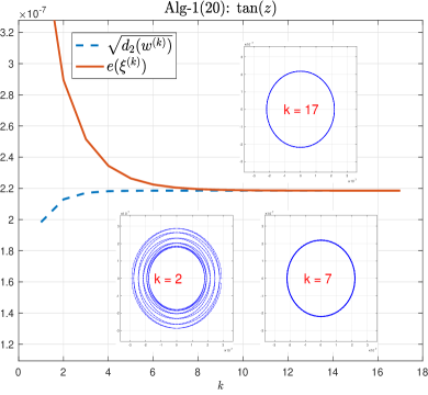
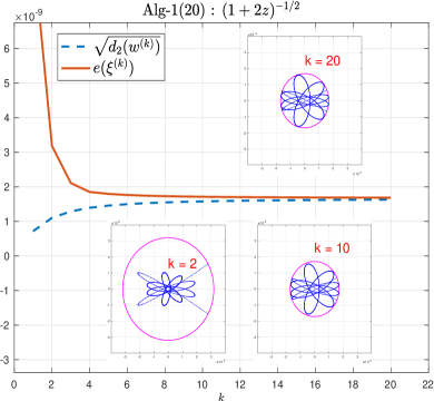
the monotonic convergence of Algorithm 1 with respect to the dual objective function value ,
-
(iii)
the weak duality as well as the strong duality (4.4) as increases,
- (iv)
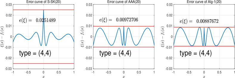
To demonstrate (i)(iii), we set (i.e., the filtering procedure in Step 2 of Algorithm 1 is inactive) for Algorithm 1. Figure 7.1 shows ( defined in (2.1) is the maximum error of the approximant ) the minimax error curves for approximating with . It can be seen that the equioscillation property is clearly observed in Alg-1(20) and AAA(20), but not in S-SK(20).
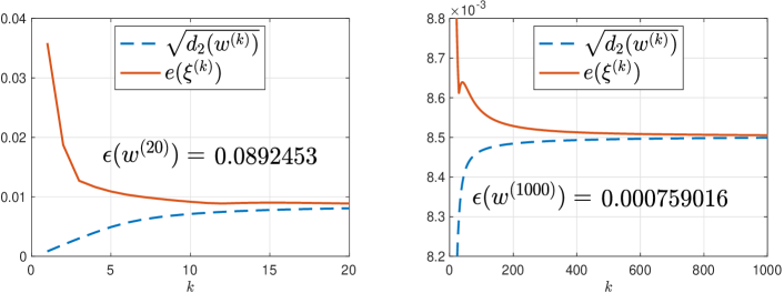
To demonstrate (ii) and (iii), we plot the sequences of and in Figure 7.2 for Algorithm 1 after a fixed number of iterations (here the computed approximant is not the one associated with the smallest described in (5) Remark 6.1). It clearly demonstrates the monotonic convergence property of , the weak duality and the strong duality (i.e., Ruttan’s sufficient condition (4.3)). The latter implies that, in this example, a best rational approximant in satisfying Ruttan’s sufficient condition (4.3) exists.
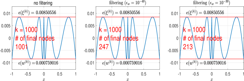
We further demonstrate (iv), i.e., the filtering procedure in Step 2 of Algorithm 1 and the theoretical result of Theorem 2.4. To this end, we choose three tolerances , , and run Algorithm 1. In Figure 7.3, we provide the error curves, the maximum error, the relative duality gap defined in (6.1) associated with the weight vector and the number of final nodes remained. It can be seen that the three approximants share the same error curve with the maximum error and the relative duality gap .
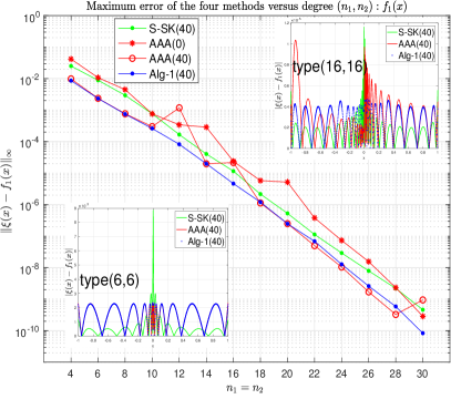
Setting for Algorithm 1, we extend the numerical test on and by varying and . Figure 7.4 provides the maximum errors of the four methods versus various diagonal types . It is observed that Alg-1(40) performs stably in computing the minimax rational approximations, and AAA(40) is also effective and very efficient to achieve the best rational approximation. In some special cases, for example, for the types and in approximating , we found that the approximants from AAA(40) are only near-best. On the other hand, we point out that AAA and AAA-Lawson are very fast as they only take within a second to return a result but Algorithm 1 and S-SK usually consume a few seconds. In addition, S-SK(40) is also able to return a good accuracy but the approximants, by checking the corresponding error curves, do not imply the equioscillation property.
| (4,4) | 0.0294 | 8.3850e-03 | 8.6391e-03 | 2.5149e-02 | 9.8259e-03 |
| (8,8) | 0.0491 | 7.1058e-04 | 7.4746e-04 | 2.9563e-03 | 7.6865e-04 |
| (12,12) | 0.1613 | 6.7055e-05 | 8.2478e-05 | 1.6777e-04 | 1.1849e-03 |
| (16,16) | 0.1391 | 3.9466e-06 | 4.6650e-06 | 1.1597e-05 | 2.1704e-05 |
| (20,20) | 0.2412 | 1.8148e-07 | 2.4819e-07 | 5.2943e-07 | 2.4997e-07 |
| (24,24) | 0.3099 | 7.5012e-09 | 1.2815e-08 | 2.9309e-08 | 1.0483e-08 |
| (28,28) | 0.3264 | 2.7869e-10 | 5.8647e-10 | 2.2062e-09 | 3.2723e-10 |
| (1,1) | 0.0201 | 4.3214e-02 | 4.4085e-02 | 1.3364e-01 | 4.3906e-02 |
| (3,3) | 0.0342 | 1.4777e-03 | 1.5283e-03 | 5.7910e-03 | 1.5644e-03 |
| (5,5) | 0.0440 | 2.3640e-05 | 2.4711e-05 | 9.8900e-05 | 2.4455e-05 |
| (7,7) | 0.0479 | 2.7952e-07 | 2.9328e-07 | 1.1603e-06 | 2.9500e-07 |
| (9,9) | 0.0547 | 2.7869e-09 | 2.9464e-09 | 1.1618e-08 | 3.0726e-09 |
| (11,11) | 0.0546 | 2.3627e-11 | 3.3090e-11 | 1.6375e-10 | 2.7122e-11 |
To demonstrate the strong duality with different for and , in Tables 7.1 and 7.2, respectively, we present the final relative duality gaps for Algorithm 1. Reported are also the maximum errors from other methods. Our further numerical experiments indicate that Ruttan’s sufficient condition (4.3) holds in all these cases (by increasing , we observed that from Algorithm 1 decreases).
7.1.2 Function with singularities on an interval
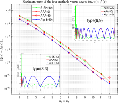
We carry out more tests for the real functions with singularities in given intervals. For this purpose, we choose the following two examples used in [16]:
In the left two subfigures of Figure 7.5, and are plotted in the given intervals; the right two subfigures of Figure 7.5 present the error curves corresponding to the types and , respectively, and the relative duality gap from Algorithm 1. In our discrete data, we set and .
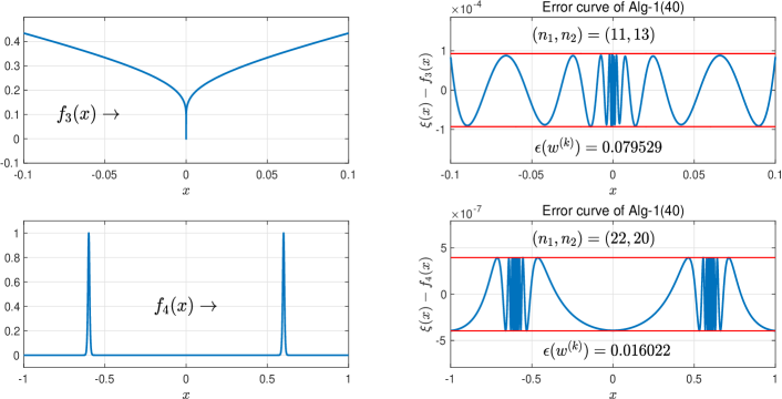
To report the results for and , we analogously choose various diagonal types and present the maximum errors in Figure 7.6. The corresponding relative duality gaps of Algorithm 1 and the maximum errors are given in Tables 7.3 and 7.4, respectively. For , we noticed that AAA(40) is unstable in some cases but the pure AAA(0) can stably provide good (non-minimax) rational approximants. For , the two singularities points certainly make the minimax rational approximation hard, and we noticed that all the methods perform unstably for some types, e.g., (14,14), (18,18) and (22,22), of . Even though it is difficult to check the existence of the minimax rational approximant and Ruttan’s sufficient condition for these cases, we can say, from the relative duality gap in Table 7.4, that these approximants from Algorithm 1 are far from the best.


| (12,12) | 0.1417 | 8.0938e-05 | 9.5057e-05 | 5.3182e-04 | 1.0244e-04 |
| (16,16) | 0.1420 | 4.0234e-06 | 5.0896e-06 | 1.1315e-05 | 5.1749e-06 |
| (20,20) | 0.2385 | 1.6587e-07 | 2.4724e-07 | 5.8103e-07 | 2.2343e-07 |
| (24,24) | 0.3697 | 5.7236e-09 | 9.5896e-09 | 3.5262e-08 | 1.7660e-06 |
| (28,28) | 0.3671 | 2.0456e-10 | 4.0257e-10 | 1.0746e-07 | 1.0470e-01 |
| (32,32) | 0.2531 | 6.7043e-12 | 1.4254e-11 | 1.0535e-10 | 1.0417e-01 |
| (16,16) | 0.0113 | 8.0564e-06 | 8.1474e-06 | 2.6195e-05 | 1.1989e-05 |
| (18,18) | 0.9776 | 9.3436e-07 | 1.0945e-03 | 1.4804e-03 | 1.6812e-04 |
| (20,20) | 0.0295 | 4.0228e-07 | 4.1424e-07 | 8.1445e-03 | 4.4159e-07 |
| (22,22) | 0.9713 | 1.1143e-07 | 2.4622e-04 | 6.8003e-05 | 2.9151e-05 |
| (24,24) | 0.0222 | 1.9999e-08 | 2.0444e-08 | 3.9508e-05 | 2.1812e-08 |
| (26,26) | 0.9499 | 5.8772e-09 | 5.2936e-07 | 1.4971e-04 | 1.8472e-06 |
7.2 Numerical experiments on complex cases
7.2.1 Analytic function on a domain
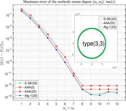
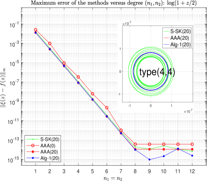
For the complex case, we first test the methods on the following two basic analytic functions [30, 39] on the unit disc. By the maximum modulus principle for analytic functions, we choose nodes on the unit circle.
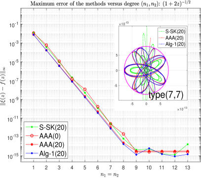
By calling the four methods on and using different diagonal types , we present the numerical results in Figure 7.7. For the two analytic functions on , the maximum error reaches the level when the degree . It seems that rounding errors play a role so that the maximum errors do not decrease as the degrees for all methods. In Tables 7.5 and 7.6, we report the relative duality gap from Algorithm 1 and the maximum errors of all methods. Note that increases significantly from to , possibly due to the effects of the rounding error.
| (1,1) | 0.0017 | 3.9727e-01 | 3.9801e-01 | 5.5728e-01 | 3.9806e-01 |
| (3,3) | 0.0006 | 6.5927e-04 | 6.5964e-04 | 6.8942e-04 | 6.5929e-04 |
| (5,5) | 0.0006 | 1.0339e-07 | 1.0345e-07 | 1.0517e-07 | 1.0339e-07 |
| (7,7) | 0.0007 | 3.6816e-12 | 3.6843e-12 | 3.7175e-12 | 3.6832e-12 |
| (9,9) | 0.1898 | 1.3614e-15 | 2.2597e-15 | 2.4931e-15 | 1.7578e-14 |
| (11,11) | 0.4116 | 1.1250e-15 | 6.3456e-15 | 7.7819e-15 | 1.7578e-14 |
| (1,1) | 0.0007 | 1.2849e-02 | 1.2859e-02 | 1.6938e-02 | 1.2854e-02 |
| (3,3) | 0.0007 | 4.5539e-06 | 4.5572e-06 | 5.9691e-06 | 4.5539e-06 |
| (5,5) | 0.0006 | 1.5094e-09 | 1.5102e-09 | 1.9784e-09 | 1.5094e-09 |
| (7,7) | 0.0010 | 4.9349e-13 | 4.9420e-13 | 6.7256e-13 | 4.9453e-13 |
| (9,9) | 0.3439 | 5.1799e-16 | 9.3054e-16 | 1.1278e-14 | 1.0785e-14 |
| (11,11) | 0.4476 | 3.9892e-16 | 1.2602e-14 | 1.1791e-14 | 1.0785e-14 |
7.2.2 Function with singularities on a domain
As our final part of numerical testing, we choose two functions and with singularities on the unit disk . In particular, [14] has a pole and [30, Fig 4.3, Sec.4] has branch point singularities on the unit disk .
The maximum errors given in Figure 7.8 again demonstrate the difficulty of computing the rational minimax approximation whenever the maximum error is near or below the machine precision for the four methods. In particular, for , the computed approximants of degrees from all the methods are not the minimax solutions of (1.2) by checking the left of Figure 7.8 and in Table 7.7. Similarly for , by investigating in Table 7.8, we know that the computed solutions with degrees are only near-best but are also good rational approximants. For Algorithm 1, increasing the number of iterations can improve the accuracy with smaller gaps (for instance, gaps for degrees get to the level of when ). Overall, Algorithm 1 turns out to be an effective approach for the rational minimax problem (1.2).

| (1,1) | 0.0416 | 7.5302e-03 | 7.8485e-03 | 1.3596e-02 | 7.7606e-03 |
| (3,3) | 0.0305 | 3.5156e-06 | 3.6250e-06 | 9.2153e-06 | 3.9042e-06 |
| (5,5) | 0.0327 | 1.6307e-09 | 1.6849e-09 | 5.1156e-09 | 2.1155e-09 |
| (7,7) | 0.0394 | 7.5464e-13 | 7.8584e-13 | 2.5965e-12 | 1.0684e-12 |
| (9,9) | 0.4221 | 5.3387e-16 | 1.3007e-15 | 4.3203e-15 | 3.1598e-15 |
| (11,11) | 0.5527 | 4.1324e-16 | 1.5144e-15 | 1.6653e-15 | 3.1598e-15 |
| (6,6) | 0.0870 | 4.0619e-03 | 4.4414e-03 | 1.0535e-02 | 4.8379e-03 |
| (10,10) | 0.2706 | 3.7903e-04 | 5.1390e-04 | 4.0039e-03 | 4.7570e-04 |
| (14,14) | 0.4855 | 4.7074e-05 | 9.3590e-05 | 4.6529e+01 | 8.2179e-05 |
| (18,18) | 0.6673 | 6.9320e-06 | 1.9569e-05 | 5.6896e-01 | 1.5388e-05 |
| (22,22) | 0.7997 | 1.1264e-06 | 5.0887e-06 | 4.8707e-01 | 5.9994e-06 |
| (26,26) | 0.8919 | 1.8130e-07 | 1.5080e-06 | 1.3732e-01 | 2.1900e-05 |
We conclude this section by emphasizing again the properties of the monotonic convergence, the weak and strong duality related with Algorithm 1 in the complex situation. These properties are closely connected to the underlying dual programming (2.11) and provide theoretical foundations for the new Lawson’s iteration. In Figure 7.9, we plot the sequences and for and with type and , respectively. Error curves in the complex plane after certain numbers of iterations are also included. We observed that the weight computed by Algorithm 1 verifies the strong duality (4.4), implying Ruttan’s sufficient condition holds and Algorithm 1 successfully solves globally the dual programming (2.11). The right subfigure also indicates that there are reference points (i.e., ) in approximating .
8 Concluding remarks and further issues
For the discrete rational minimax approximation (1.2), in this paper, we have proposed a convex optimization (2.11) over the probability simplex and designed correspondingly a new version of Lawson’s iteration (Algorithm 1). The convex programming (2.11) is derived as a dual programming of a certain linearized reformulation of the rational minimax approximation. We showed that there is no duality gap between the primal and the dual under Ruttan’s sufficient condition. In practice, Ruttan’s sufficient condition, or equivalently, the strong duality, is checkable through (4.4) after solving the dual programming (2.11) globally. The relative duality gap also reflects the accuracy of the minimax approximant. Our numerical experiments indicate that the easily-implementable Lawson’s iteration (Algorithm 1) is an effective approach for solving the convex programming (2.11).
Even the dual programming (2.11) can provide a new perspective for the rational minimax approximation (1.2), several important issues have not been discussed in this paper. Indeed, the observed linear and monotonic convergence in our numerical experiments of the new Lawson’s iteration has not been established in theory. As pointed out in [30] for AAA-Lawson that ‘it is a challenge for the future to develop further improvements to the algorithm that might ensure its convergence in all circumstances and to support these with theoretical guarantees’, we think an associated dual problem can play a role to analyze the theoretical convergence of the corresponding Lawson’s iteration. To improve the stability of Algorithm 1, barycentric representations, instead of the Vandermonde basis, may also be employed for solving dual programming (2.11). Moreover, the present new Lawson’s iteration can also fail to solve the dual (2.11) globally (i.e., the duality gap does not converge to zero), and even it converges, the convergence in some cases can be slow and less efficient than the AAA, AAA-Lawson algorithm. Fast and effective methods for globally solving the dual programming are certainly desired as detecting the reference points (i.e., nodes in of (2.10)) corresponds to finding the nonzero weights at the maximizer of the dual programming (2.11); reference points are helpful in the representation of either by finding roots [23] of and , or their associated coefficient vectors in certain bases. As the dual (2.11) is to maximize a concave function over the probability simplex and both the gradient and the Hessian of are provided in section 5, other methods, including the projected gradient iteration, the interior-point method [32, Chapter 19] or other methods for convex optimization [31], can be applied for solving (2.11). All theses issues deserve further investigations.
References
- [1] N. I. Akhiezer, Elements of the Theory of Elliptic Functions, Transl. Math. Monogr. 79, American Mathematical Society, Providence, RI, 1990.
- [2] I. Barrodale and J. Mason, Two simple algorithms for discrete rational approximation, Math. Comp., 24 (1970), 877–891.
- [3] I. Barrodale, M. J. D. Powell and F. D. K. Roberts, The differential correction algorithm for rational approximation, SIAM J. Numer. Anal., 9 (1972), 493–504.
- [4] M. Berljafa and S. Güttel, Generalized rational Krylov decompositions with an application to rational approximation, SIAM J. Matrix Anal. Appl., 36 (2015), 894–916, URL https://doi.org/10.1137/140998081.
- [5] M. Berljafa and S. Güttel, The RKFIT algorithm for nonlinear rational approximation, SIAM J. Sci. Comput., 39 (2017), A2049–A2071, URL https://doi.org/10.1137/15M1025426.
- [6] S. Boyd and L. Vandenberghe, Convex Optimization, Cambridge University Press, 2004.
- [7] P. D. Brubeck, Y. Nakatsukasa and L. N. Trefethen, Vandermonde with Arnoldi, SIAM Rev., 63 (2021), 405–415.
- [8] E. W. Cheney and H. L. Loeb, Two new algorithms for rational approximation, Numer. Math., 3 (1961), 72–75.
- [9] A. K. Cline, Rate of convergence of Lawson’s algorithm, Math. Comp., 26 (1972), 167–176.
- [10] P. Cooper, Rational approximation of discrete data with asymptotic behaviour, PhD thesis, University of Huddersfield, 2007.
- [11] J. W. Demmel, M. Gu, S. Eisenstat, I. Slapničar, K. Veselić and Z. Drmač, Computing the singular value decomposition with high relative accuracy, Linear Algebra Appl., 299 (1999), 21–80.
- [12] J. W. Demmel and K. Veselić, Jacobi’s method is more accurate than QR, SIAM J. Matrix Anal. Appl., 13 (1992), 1204–1245.
- [13] T. A. Driscoll, N. Hale and L. N. Trefethen, Chebfun User’s Guide, Pafnuty Publications, Oxford, 2014, See also www.chebfun.org.
- [14] S. Ellacott and J. Williams, Linear Chebyshev approximation in the complex plane using Lawson’s algorithm, Math. Comp., 30 (1976), 35–44.
- [15] G. H. Elliott, The construction of Chebyshev approximations in the complex plane, PhD thesis, Facultyof Science (Mathematics), University of London, 1978.
- [16] S.-I. Filip, Y. Nakatsukasa, L. N. Trefethen and B. Beckermann, Rational minimax approximation via adaptive barycentric representations, SIAM J. Sci. Comput., 40 (2018), A2427–A2455.
- [17] G. H. Golub and C. F. Van Loan, Matrix Computations, 4th edition, Johns Hopkins University Press, Baltimore, Maryland, 2013.
- [18] I. V. Gosea and S. Güttel, Algorithms for the rational approximation of matrix-valued functions, SIAM J. Sci. Comput., 43 (2021), A3033–A3054, URL https://doi.org/10.1137/20M1324727.
- [19] B. Gustavsen and A. Semlyen, Rational approximation of frequency domain responses by vector fitting, IEEE Trans. Power Deliv., 14 (1999), 1052–1061.
- [20] M. H. Gutknecht, On complex rational approximation. Part I: The characterization problem, in Computational Aspects of Complex Analysis (H. Werneret at.,eds.). Dordrecht : Reidel, 1983, 79–101.
- [21] J. M. Hokanson, Multivariate rational approximation using a stabilized Sanathanan-Koerner iteration, 2020, URL arXiv:2009.10803v1.
- [22] M.-P. Istace and J.-P. Thiran, On computing best Chebyshev complex rational approximants, Numer. Algorithms, 5 (1993), 299–308.
- [23] S. Ito and Y. Nakatsukasa, Stable polefinding and rational least-squares fitting via eigenvalues, Numer. Math., 139 (2018), 633–682.
- [24] C. L. Lawson, Contributions to the Theory of Linear Least Maximum Approximations, PhD thesis, UCLA, USA, 1961.
- [25] X. Liang, R.-C. Li and Z. Bai, Trace minimization principles for positive semi-definite pencils, Linear Algebra Appl., 438 (2013), 3085–3106.
- [26] H. L. Loeb, On rational fraction approximations at discrete points, Technical report, Convair Astronautics, 1957, Math. Preprint #9.
- [27] R. D. Millán, V. Peiris, N. Sukhorukova and J. Ugon, Application and issues in abstract convexity, 2022, URL arXiv:2202.09959.
- [28] R. D. Millán, V. Peiris, N. Sukhorukova and J. Ugon, Multivariate approximation by polynomial and generalised rational functions, Optimization, 71 (2022), 1171–1187.
- [29] Y. Nakatsukasa, O. Sète and L. N. Trefethen, The AAA algorithm for rational approximation, SIAM J. Sci. Comput., 40 (2018), A1494–A1522.
- [30] Y. Nakatsukasa and L. N. Trefethen, An algorithm for real and complex rational minimax approximation, SIAM J. Sci. Comput., 42 (2020), A3157–A3179.
- [31] Y. Nesterov, Lectures on Convex Optimization, 2nd edition, Springer, 2018.
- [32] J. Nocedal and S. Wright, Numerical Optimization, 2nd edition, Springer, New York, 2006.
- [33] J. R. Rice, The approximation of functions, Addison-Wesley publishing Company, 1969.
- [34] A. Ruttan, A characterization of best complex rational approximants in a fundamental case, Constr. Approx., 1 (1985), 287–296.
- [35] E. B. Saff and R. S. Varga, Nonuniqueness of best approximating complex rational functions, Bull. Amer. Math. Soc., 83 (1977), 375–377.
- [36] C. K. Sanathanan and J. Koerner, Transfer function synthesis as a ratio of two complex polynomials, IEEE T. Automat. Contr., 8 (1963), 56–58, URL https://doi.org/10.1109/TAC.1963.1105517.
- [37] J.-P. Thiran and M.-P. Istace, Optimality and uniqueness conditions in complex rational Chebyshev approximation with examples, Constr. Approx., 9 (1993), 83–103.
- [38] L. N. Trefethen, Approximation Theory and Approximation Practice, Extended Edition, SIAM, 2019.
- [39] J. Williams, Numerical Chebyshev approximation in the complex plane, SIAM J. Numer. Anal., 9 (1972), 638–649.
- [40] J. Williams, Characterization and computation of rational Chebyshev approximations in the complex plane, SIAM J. Numer. Anal., 16 (1979), 819–827.
- [41] D. E. Wulbert, On the characterization of complex rational approximations, Illinois J. Math., 24 (1980), 140–155.
- [42] L. Yang, L.-H. Zhang and Y. Zhang, The Lq-weighted dual programming of the linear Chebyshev approximation and an interior-point method, 2023, URL https://www.researchgate.net/publication/368987000_The_Lq-weighted_dual_programming_of_the_linear_Chebyshev_approximation_and_an_interior-point_method, Preprint.
- [43] L.-H. Zhang, Y. Su and R.-C. Li, Accurate polynomial fitting and evaluation via Arnoldi, Numerical Algebra, Control and Optimization, to appear, Doi:10.3934/naco.2023002.