Exact Inequality and the Absence of Floating Phase in a Superconductor with Time-reversal Symmetry Breaking on any Lattice

Abstract

Due to the interplay of multi-component order parameters (e.g., a bilayer superconductor with vanishing 1^st order Josephson tunneling [1] or a frustrated $n\geq 3$-band superconductor [2]), a superconductor can possess a $U(1)\times\mathbb{Z}_{2}$ symmetry, corresponding to the superconducting $T_{c}$ and time-reversal symmetry breaking transition $T_{\text{TRSB}}$, respectively. It was then conjectured that in vast parameter regimes (schematically denoted by $J_{2}$) and spatial dimensions $d$, there is only a single phase transition, i.e., $T_{c}=T_{\text{TRSB}}$. Mathematically, the conjecture is equivalent to the following two properties being true simultaneously: (1) the absence of a floating phase $T_{\text{TRSB}}\geq T_{c}$ and (2) the absence of vestigial TRSB $T_{\text{TRSB}}\leq T_{c}$. In this paper, we study the system in the strong coupling limit $J_{2}\to\infty$. By using exact dual graphical representations, we provide 2 independent proofs showing that the correlation functions of $U(1)$ spins is bounded above by that of $\mathbb{Z}_{2}$ spins for all temperatures and lattice structures (e.g., $\mathbb{Z}^{d}$ for all $d$). In particular, this implies that property (1) must hold true on any lattice structure and thus guarantees the existence of high $T_{c}$ TRSB superconductivity. Further implications of this correlation inequality (such as whether the conjectured single transition is first/second order) are also discussed.

I Introduction

In the last seveal years, there has been considerable excitement generated by various theoretical [3, 4, 5, 6, 7, 8, 2] and experimental [9, 10, 11, 12] proposals concerning the existence of time-reversal symmetry breaking (TRSB) pairing states in various unconventional superconductors. However, conclusive experimental evidence of these states has not so far been reported.

Recently, it was proposed that high-$T_{c}$ topological superconductivity can be reliably achieved via twisting two identical 2D layers of BSCCO ($d_{x^{2}-y^{2}}$-wave pairing symmetry) relative to each other [1]. At relative orientation $\pi/4$, the 1^st order inter-layer Josephson coupling $J_{1}$ vanishes so that the 2^nd order coupling $J_{2}$ (with a sign that favors an inter-layer phase difference $=\pm\pi/2$) becomes the dominant inter-layer interaction. This inter-layer term was conjectured to induce a TRSB transition ($d_{x^{2}-y^{2}}\pm id_{xy}$ state) with a critical temperature that is on the same order as the superconducting transition, i.e., $T_{\text{TRSB}}\approx T_{c}$, and thus generating high $T_{c}$ topological superconductivity (albeit with a gap magnitude proportional to $J_{2}$, which in the actual system is expected to be very small [8].).

Alternatively, it was proposed that in a $(n\geq 3)$-band superconductor, the inter-band 1^st order Josephson coupling can cause sufficient frustration among the inter-band phase differences so that the ground state configurations may exhibit phase differences which differ from 0 or $\pi$ and thus result in TRSB [2]. Such a proposal is especially enticing since it is not limited to 2D layers and may also circumvent the issue of a small gap magnitude in the previous proposal. Similar proposals have been argued to occur in the hole doped Ba_1-xK_xFe₂As₂ pnictide superconductor [13] and other classes of materials [14, 15, 16, 17, 18].

In both scenarios, the system possesses a $U(1)\times\mathbb{Z}_{2}$ symmetry, corresponding to the superconducting $T_{c}$ and TRSB transition $T_{\text{TRSB}}$, respectively. To achieve high $T_{c}$ topological superconductivity, it is imperative that the TRSB transition occurs on the same order as the superconducting transition $T_{\text{TRSB}}\approx T_{\text{c}}$. In fact, it was conjectured that at critical values (e.g., $J_{1}=0$ in the former 2D bilayer BSCCO scenario), the two transitions coincide exactly $T_{c}=T_{\text{TRSB}}$ for vast parameter regimes (e.g., $J_{2}>0$) and spatial dimensions $d$.

Within the context of different types of mean-field theory applied either to a Ginzburg-Landau effective field theory [1, 19, 13] or an XY model on a regularized lattice [20, 21], the conjecture is understood and holds true. However, it is well known that mean-field theory is quantitatively reliable only when the effective number of neighboring spins is large as occurs when there are long-range interactions or in high dimensions (generally believed to be $d\geq 4$). In low dimension ($d=2,3$) systems, fluctuations due to local nearest-neighbor interactions may play an important fact. Due to the lack of exact results in low dimensions, it is then conventional to rely on numerical evidence (in 2D [22] and in 3D [23, 2]) and RG calculations (in 2D [24]) to provide us insight into the problem. Unfortunately, in this scenario, the distinct approaches contradict with each other: numerical evidence agrees with the conjecture, while latter RG calculations suggest a vestigial TRSB phase $T_{\text{TRSB}}>T_{c}$ (although further detailed RG calculations seem to reconcile this matter [25]). Therefore, the main goal of this paper is to obtain exact results on the short-range nearest-neighbor model.

Mathematically, the conjecture $T_{\text{TRSB}}=T_{c}$ is equivalent to the following two properties being true simultaneously:

1. The absence of a floating phase, $T_{\text{TRSB}}\geq T_{c}$.

2. The absence of vestigial TRSB, $T_{\text{TRSB}}\leq T_{c}$.

In this paper, we shall consider the strong coupling limit (e.g., $J_{2}\to\infty$ in the 2D bilayer BSCCO scenario), and provide 2 distinct proofs showing that property (1) holds true not only for the translationally invariant cases studied on $\mathbb{Z}^{d}$, but also for any lattice structure with arbitrary nearest-neighbor interaction strengths. This guarantees the existence of high $T_{c}$ superconductivity with TRSB and possibly topological superconductivity. More specifically, we prove that the correlation functions of $U(1)$ spins is bounded above by that of $\mathbb{Z}_{2}$ spins for all temperatures and lattice structures (e.g., $\mathbb{Z}^{d}$ for all $d$, triangular or kagome lattices, etc.). Further implications of this correlation inequality (such as whether the conjectured single transition is first/second order) are also discussed.

It should be noted that we do not have a proof for property (2) and thus cannot reconcile the previously discussed contradiction between numerical and RG calculations. However, we shall provide insight into property (2) by considering the closely related $\mathbb{Z}_{4}\times\mathbb{Z}_{2}$ and $\mathbb{Z}_{2}\times\mathbb{Z}_{2}$ models, in which the $U(1)$ spins are replaced by the $\mathbb{Z}_{4}$ and $\mathbb{Z}_{2}$ clock models, respectively. In these simplified models, the short-range interaction is preserved, yet we can prove rigorously that there is only a single phase transition on any lattice structure. This raises concerns towards the claims of Ref. [24] on vestigial order.

The paper is organized as follows. Sec. (II) introduces the classical statistical model under investigation as well as its motivation, i.e., twisted bilayer BSCCO and frustrated $(n\geq 3)$-band superconductors. We also provide a quick sketch of subtle mathematical regularizations necessary to define the thermodynamic limit on a general lattice structure. Sec. (III) introduces the (random) cluster representation, which is an exact dual graphical representation closely related to the Wolff algorithm that will be used to provide our first proof of the main result (1). Sec. (IV) introduces the (random) current representation, which is another exact dual graphical representation that will act as our second proof of the main result. We emphasize that the two proofs are independent of each other and thus result in slightly different conclusions, i.e., Theorem (1) vs. (2). Each proof has their own advantages and disadvantages, which we will discuss explicitly in Sec. (V). Further implications of our main result (other than showing that property (1) holds true) is also discussed in this section. In Sec. (VI), we shall consider the previously discussed $\mathbb{Z}_{4}\times\mathbb{Z}_{2}$ and $\mathbb{Z}_{2}\times\mathbb{Z}_{2}$ models, and prove that the conjecture (property (1) and (2)) holds true for these simplified models on any lattice structure. Although this does not necessarily imply whether the full $U(1)\times\mathbb{Z}_{2}$ model has similar properties, the simplified structures should be regarded as toy models providing insight towards the problem. The paper will only outline and cite the necessary theorems, while leaving the proof in the Appendix.

II Model

For the majority of this paper, we shall consider the following classical statistical $U(1)\times\mathbb{Z}_{2}$ Hamiltonian

$$H(\sigma,\tau)=-\sum_{e=ij}\kappa_{e}(1+\tau_{i}\tau_{j})\sigma_{i}\cdot\sigma_{j}$$ (1)

where the summation is over all nearest-neighbors (edges $e=ij$) on a graph and $\kappa_{e}\geq 0$ denote arbitrary ferromagnetic coupling constants on each edge $e$. Moreover, $\tau_{i}=\pm 1$ denotes the $\mathbb{Z}_{2}$ Ising spins corresponding to TRSB, while $\sigma_{i}=e^{i\theta_{i}}\in\mathbb{S}^{1}\cong\mathbb{C}$ denotes the $U(1)$ XY spins corresponding to superconductivity. Note that the Hamiltonian can be defined on any graph $G$.

II.1 Motivation: The Strong Coupling Limit

We now show that the Hamiltonian in Eq. (1) with constant $\kappa_{e}=1$ describes the strong coupling limit of the previously mentioned motivations, i.e., twisted bilayer BSCCO with only 2^nd order Josephson coupling and the $(n\geq 3)$-band superconductor with frustrated inter-band 1^st Josephson coupling. Indeed, the latter was derived in Ref. [2]; our Hamiltonian with constant $\kappa_{e}=1$ corresponds to Eq. (8) of Ref. [2] at the critical point of $K_{1}=1,K_{2}=0$. Similarly, in the former scenario, one can model the 2D layers via identical standard XY models, coupled by a 2^nd order Josephson coupling $J_{2}\geq 0$, i.e.,

$$H_{J_{2}}(\phi^{\pm})=\sum_{\ell=\pm}H^{\text{XY}}(\phi^{\ell})+J_{2}\sum_{i}\cos 2\phi_{i}$$ (2)

Where $\phi^{\pm}$ denotes the phases of the XY spins in each layer and $\phi\equiv\phi^{+}-\phi^{-}$ denotes the phase difference across the junction. In this model, it is clear that for any $J_{2}>0$, the Hamiltonian is minimized when the phase difference $\phi$ chooses between $\pm\pi/2$ and thus the $\mathbb{Z}_{2}$ Ising order corresponds to TRSB $T_{\text{TRSB}}$. Moreover, if we take the strong coupling limit $J_{2}\to\infty$ [26], the phase difference $\phi$ is forced to choose between $\pm\pi/2$ at each lattice site $i$ and thus induces an explicit $\mathbb{Z}_{2}$ Ising order, i.e., $\phi_{i}=\tau_{i}\times\pi/2$ where $\tau_{i}=\pm 1$. On the other hand, the average phase $\theta=(\phi^{+}+\phi^{-})/2$ is unrestricted and thus induces a $U(1)$ XY spin $\sigma_{i}=e^{i\theta_{i}}$ corresponding to the superconducting transition $T_{c}$. Using this change of variables, the Hamiltonian in Eq. (2) reduces to Eq. (1) with $\kappa_{e}=1$ in the strong coupling limit $J_{2}\to\infty$.

One may also wonder why we should study the strong coupling limit, since it “appears” to be a singular point. Apart from simplifying the problem, one reason is that the strong coupling limit is not singular; rather, it is continuously connected to large but finite coupling strengths in the sense of correlation functions as argued previously [26]. Moreover, the authors of Ref. [2] numerically studied the strong coupling model (with constant $\kappa_{e}=1$) on the 3D cubic lattice, and showed that the phase diagram does not change qualitatively as we leave the strong coupling regime. Similar numerical results [22] were also performed in 2D, in which it was shown that the phase diagram is insensitive to the actual values of the coupling strength $J_{2}$ (though they did not investigate the strong coupling limit). In higher dimension $d\geq 4$, mean-field theory predicts a similar behavior [8, 1], and thus we believe that studying the strong coupling limit can reflect the properties of the finite coupling model, though admittedly, this is not determined definitively.

II.2 Regularization and the Thermodynamic Limit

It should be noted that the Hamiltonian in Eq. (1) is only well-defined on a finite graph $G=(V,E)$ where $V$ denotes the finite number of lattice sites and $E$ denotes the possible edges. To take the thermodynamic limit, the convention is to

1. Fix an infinite graph $G_{\infty}=(V_{\infty},E_{\infty})$, e.g., the standard $\mathbb{Z}^{d}$, with edge couplings $\kappa:E_{\infty}\to[0,\infty)$;

2. Study systems on finite subgraphs $G=(V,E)$ with thermal averages $\langle\cdots\rangle_{G}$, e.g., finite boxes $\Lambda_{L}=\{-L,...,L\}^{d}\subseteq\mathbb{Z}^{d}$;

3. And take the limit as $G\nearrow G_{\infty}$ exhausts the infinite graph (e.g., $L\to\infty$), where the existence of the limit also needs to be proved.

In the case of the $U(1)\times\mathbb{Z}_{2}$ Hamiltonian in Eq. (1), the system is fully ferromagnetic ($\kappa_{e}\geq 0$ for all edges $e$) and thus Ginibre’s inequality can be applied [27], so that correlation functions

$$\langle\tau_{0}\tau_{R}\rangle_{G},\quad\langle\cos 2(\theta_{0}-\theta_{R})\rangle_{G}=\langle\sigma_{0}^{2}\bar{\sigma}_{R}^{2}\rangle_{G}$$ (3)

Are monotonically increasing as the subgraph $G$ increases, and thus their thermodynamic limits $G\nearrow G_{\infty}$ are well-defined since they are bounded above by $\leq 1$.

It should be noted that, in this paper, we shall study the high-order $U(1)$ correlations $\langle\cos 2(\theta_{0}-\theta_{R})\rangle$ rather than the conventional correlations $\langle\cos(\theta_{0}-\theta_{R})\rangle$. Apart from our inability to produce useful inequalities regarding the latter correlations, there is a physically relevant reason towards this perspective. Indeed, as discussed previously, $\theta$ is physically related to the average phase of independent XY spins, i.e., $\theta=(\phi^{+}+\phi^{-})/2$. However, notice that $\cos\theta$ is not invariant under rotation $\phi^{+}\mapsto\phi^{+}+2\pi$, and thus, in this sense, the $2\pi$-invariant higher order term $\cos(2\theta)$ is the physically relevant term to consider.

III Random Cluster Representation

The cluster representation dates back to Fortuin and Kasteleyn [28], where it was originally developed to study the Ising and more generally, the $q$-state Potts model. The correspondence between phase transitions in spin models and percolation in the corresponding cluster representation has proven useful in numerous occasions in obtaining rigorous results [29, 30, 31, 32, 33]. Numerically, the correspondence has allowed the closely related Wolff algorithm to take advantage of non-local cluster spin updates, in contrast to local spin flips as in the Metropolis-Hasting algorithm [34]. In some sense, the Wolff algorithm provides an alternative (and possibly more familiar) perspective in constructing the cluster representation and thus we will provide a short review using the example of the standard Ising model.

III.1 Short Review of the Wolff Algorithm

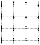
(a)

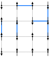
(b)

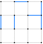
(c)

Figure 1: Cluster Representation on $\mathbb{Z}^{2}$. (a). Some Ising spin configuration chosen from the Ising Gibbs state. (b). A constructed subgraph $\omega$ based on the Ising spin configuration in Fig. 1a. Note that not all ordered edges are included in $\omega$, since an edge $e$ is included with some probability. However, all disordered edges are not included (based on the edge probability defined in Eq. (6)). (c). The subgraph after integrating over all possible spin configurations.

The standard Ising model on a finite graph $G$,

$$H^{\text{Is}}(\tau)=-\sum_{e=ij}\tau_{i}\tau_{j}$$ (4)

Defines a probability distribution over Ising spin configurations, i.e.,

$$\mathbb{P}^{\text{Is}}[\tau]\propto\prod_{e=ij}w^{\text{Is}}_{e}(\tau),\quad w_{e}^{\text{Is}}(\tau)=e^{\beta\tau_{i}\tau_{j}}$$ (5)

Where the product is over all edges with a weight $w_{e}^{\text{Is}}$ that depends on the spin configuration $\tau$ implicitly through its values on the endpoints $i,j$ of edge $e$.

Given a fixed spin configuration $\tau$ (see Fig. 1a), the Wolff algorithm then generates a subgraph $\omega:E\to\{0,1\}$ in the following manner. Let

$$p_{e}^{\text{Is}}(\tau)=\left[1-\frac{w_{e}^{\text{Is}}(\tau^{i})}{w_{e}^{\text{Is}}(\tau)}\right]1\{\tau_{i}\tau_{j}=+1\}$$ (6)

Where $\tau^{i}$ is the spin configuration derived from $\tau$ by flipping $\tau_{i}\mapsto-\tau_{i}$ (where $i$ is an endpoint of edge $e$) and keeping all other spins the same. As shown in Fig. 1b, each edge $e$ is included in the subgraph $\omega$, i.e., $\omega_{e}=1$ with probability $p_{e}^{\text{Is}}(\tau)$ (otherwise, set $\omega_{e}=0$). Note that the procedure for each edge $e$ is independent of each other (conditionally independent with respect to the fixed spin configuration $\tau$) and thus defines a probability distribution on subgraphs $\omega$ and spin configurations $\tau$, i.e.,

$$\mathbb{P}^{\text{Is}}[\omega|\tau] =\prod_{e\in\omega}p_{e}^{\text{Is}}(\tau)\prod_{e\notin\omega}(1-p_{e}^{\text{Is}}(\tau))$$ (7)

$$\mathbb{P}^{\text{Is}}[(\omega,\tau)] =\mathbb{P}^{\text{Is}}[\omega|\tau]\mathbb{P}^{\text{Is}}[\tau]$$ (8)

By integrating over all spin configurations $\tau$, one then obtains the cluster representation, i.e., a probability distribution over subgraphs of the system (see Fig. 1c)

$$\mathbb{P}^{\text{Is}}[\omega]=\sum_{\tau}\mathbb{P}^{\text{Is}}[(\omega,\tau)]$$ (9)

In language of the Wolff algorithm and Monte Carlo [34], the edge probabilities $p_{e}^{\text{Is}}(\tau)$ are chosen to satisfy detailed balance. In language of probability theory, the edge probabilities are chosen so that the operation of flipping all spins in a cluster keeps the probability distribution invariant [35, 29], i.e.,

$$\mathbb{P}^{\text{Is}}[(\omega,\tau)]=\mathbb{P}^{\text{Is}}[(\omega,\tau^{C(\omega)})]$$ (10)

Where $C(\omega)$ is some cluster in $\omega$ that has been chosen to be flipped and $\tau^{C(\omega)}$ is obtained from the original spin configuration $\tau$ via flipping all spins in $C(\omega)$, i.e., $\tau_{i}\mapsto-\tau_{i}$ for all $i\in C(\omega)$, and keep all remaining spins the same.

The property of cluster-flip invariance allows us to further prove that the correlation functions are in 1-1 correspondence with percolation events in the cluster representation [29, 35], i.e.,

$$\langle\tau_{0}\tau_{R}\rangle^{\text{Is}}_{G,\beta}=\mathbb{P}_{G,\beta}^{\text{Is}}[0\leftrightarrow_{\omega}R]$$ (11)

where $\{0\leftrightarrow_{\omega}R\}$ is the event of all subgraphs $\omega$ which connect lattice sites $0,R$, and we have added the subscripts to denote dependence of inverse temperature $\beta$ and graph $G$.

Indeed, the argument is quite straightforward. Note that

$$\langle\tau_{0}\tau_{R}\rangle^{\text{Is}}=\mathbb{E}^{\text{Is}}[\tau_{0}\tau_{R}(1\{0\leftrightarrow_{\omega}R\}+1\{0\not\leftrightarrow_{\omega}R\})]$$ (12)

If $\{0\leftrightarrow_{\omega}R\}$, then by the definition of the edge probability $p_{e}^{\text{Is}}$ (if an edge is included, the edge is ordered), we see that $\tau_{0}\tau_{R}=1$. Conversely, if $\{0\not\leftrightarrow_{\omega}R\}$, then we can flip the spins $\tau$ in the cluster of $\omega$ containing lattice site 0, so that $\tau_{0}\mapsto-\tau_{0}$ but $\tau_{R}\mapsto\tau_{R}$. Since this operation leaves the probability invariant, we see that

$$\mathbb{E}^{\text{Is}}[\tau_{0}\tau_{R}1\{0\not\leftrightarrow_{\omega}R\}]=-\mathbb{E}^{\text{Is}}[\tau_{0}\tau_{R}1\{0\not\leftrightarrow_{\omega}R\}]=0$$ (13)

The correlation-percolation correspondence is thus established.

III.2 Application to the $U(1)\times\mathbb{Z}_{2}$ Model

The cluster representation was later generalized to the XY model (and more generally to $O(n)$ models) [36] roughly two decades ago. By noticing that the sign $\xi$ of the $x$-component $\cos\theta$ of the XY spins can be used as a “substitute” of the Ising spin in the cluster representation, the author established the correspondence between conventional correlations $\langle\cos(\theta_{0}-\theta_{R})\rangle^{\text{XY}}$ and percolation (analogous to Eq. (11)). However, despite the straightforward generalization of the Wolff algorithm to the standard XY model, it wasn’t until recently [35] was there significant progress on establishing a similar correspondence for the higher-order correlation $\langle\cos 2(\theta_{0}-\theta_{R})\rangle^{\text{XY}}$.

The philosophy and techniques developed for the standard Ising and XY models can thus be straightforwardly extended to the $U(1)\times\mathbb{Z}_{2}$ Hamiltonian in Eq. (1) (see Appendix (B) for explicit details). The only difficulty lies in finding a relation (inequality) between the percolation events so that

Theorem 1 (see Appendix (B)).

Let the $U(1)\times\mathbb{Z}_{2}$ Hamiltonian $H$ in Eq. (1) be defined on a finite graph $G$. Then for any temperature

$$\langle\cos 2(\theta_{0}-\theta_{R})\rangle_{G,\beta}\leq 2\langle\tau_{0}\tau_{R}\rangle_{G,\beta}$$ (14)

Sketch of Proof.

To be concrete, the Hamiltonian in Eq. (1) defines a probability distribution over spin configurations, i.e.,

$$\mathbb{P}[(\sigma,\tau)] \propto\prod_{e=ij}w_{e}(\sigma,\tau)$$ (15)

$$w_{e}(\sigma,\tau) =e^{\beta\kappa_{e}(1+\tau_{i}\tau_{j})\cos(\theta_{i}-\theta_{j})}$$ (16)

Given a fixed spin configuration $\sigma,\tau$, we can generate a subgraph $\hat{\tau}:E\to\{0,1\}$ using the edge probabilities (see also explicit form in Eq. (140))

$$p_{e}^{\tau}(\sigma,\tau)=\left[1-\frac{w_{e}(\sigma,\tau^{i})}{w_{e}(\sigma,\tau)}\right]1\{w_{e}(\sigma,\tau^{i})<w_{e}(\sigma,\tau)\}$$ (17)

We can then define a probability distribution $\mathbb{P}[(\hat{\tau},\sigma,\tau)]$ as previously discussed in Sec. (III.1), and establish the correspondence between correlations $\langle\tau_{0}\tau_{R}\rangle$ and percolation $\mathbb{P}[0\leftrightarrow_{\hat{\tau}}R]$, analogous to Eq. (11).

Similarly, we can generate a subgraph $\hat{\sigma}$ using the edge probabilities [35] (see also explicit form in Eq. (141))

$$p_{e}^{\sigma}(\sigma,\tau) =\left[1+\frac{w_{e}(\sigma^{\xi\eta,i},\tau)}{w_{e}(\sigma,\tau)}\right.$$ (18)

$$\quad\left.-\frac{w_{e}(\sigma^{\xi,i},\tau)}{w_{e}(\sigma,\tau)}-\frac{w_{e}(\sigma^{\eta,i},\tau)}{w_{e}(\sigma,\tau)}\right]$$

$$\quad\times 1\{w_{e}(\sigma^{\xi,i},\tau),w_{e}(\sigma^{\eta,i},\tau)<w_{e}(\sigma,\tau)\}$$

Where $\xi,\eta=\pm 1$ denote the signs of the $x,y$ components of the XY spin $\sigma=e^{i\theta}$, and $\sigma^{\xi,i}$ denotes the spin configuration derived from $\sigma$ by flipping the spin at site $i$ along the $x$-component, i.e., $\xi_{i}\mapsto-\xi_{i}$ or $\theta_{i}\mapsto\pi-\theta_{i}$, and keeping all other sites the same. We similarly define $\sigma^{\eta,i}$ (via $\theta_{i}\mapsto-\theta_{i}$) and $\sigma^{\xi\eta,i}$ (via $\theta_{i}\mapsto\theta_{i}+\pi$). We then define a probability distribution $\mathbb{P}[(\hat{\sigma},\sigma,\tau)]$ as before, and establish the correspondence between correlations $\langle\cos 2(\theta_{0}-\theta_{R})\rangle$ and percolation $\mathbb{P}[0\leftrightarrow_{\hat{\tau}}R]$.

Note that in our construction, we extended the probability distribution $\mathbb{P}$ over spin configurations to either that of $(\hat{\tau},\sigma,\tau)$ or $(\hat{\sigma},\sigma,\tau)$. However, if we wish to compare the (probability of) percolation events $\mathbb{P}[0\leftrightarrow_{\hat{\tau}}R]$ and $\mathbb{P}[0\leftrightarrow_{\hat{\sigma}}R]$, it is necessary to extend the probability distribution $\mathbb{P}$ to that of $(\hat{\sigma},\hat{\tau},\sigma,\tau)$, or simply that of $(\hat{\sigma},\hat{\tau})$ after integrating over all spin configurations.

One way that has turned out to be useful is to consider the conditional probability with respect to fixed spin configuration $\sigma,\tau$. Since each edge $e$ is constructed independently, we shall consider a fixed edge $e=ij$ so that $\hat{\tau}_{e},\hat{\sigma}_{e}=0,1$ correspond to Bernoulli random variables. To extend the conditional probability to both $(\hat{\sigma},\hat{\tau})$, we must define a correlation $c_{e}(\sigma,\tau)$ between the two variables so that the following probability is well-defined, i.e., the following probabilities are all $\geq 0$

$$\mathbb{P}[\hat{\sigma}_{e}=1,\hat{\tau}_{e}=1|\sigma,\tau] =c_{e}$$ (19)

$$\mathbb{P}[\hat{\sigma}_{e}=0,\hat{\tau}_{e}=1|\sigma,\tau] =p_{e}^{\tau}-c_{e}$$ (20)

$$\mathbb{P}[\hat{\sigma}_{e}=1,\hat{\tau}_{e}=0|\sigma,\tau] =p_{e}^{\sigma}-c_{e}$$ (21)

$$\mathbb{P}[\hat{\sigma}_{e}=0,\hat{\tau}_{e}=0|\sigma,\tau] =1-p_{e}^{\tau}-p_{e}^{\sigma}+c_{e}$$ (22)

If such a condition is satisfied by choosing the correlation $c_{e}$ appropriately, then by integrating over say, $\hat{\tau}_{e}=0,1$, the conditional probability of $\hat{\sigma}_{e}$ (with respect to the fixed spin configuration $(\sigma,\tau)$) will be exactly what was required, i.e., $p_{e}^{\sigma}$.

Indeed, the key observation is to notice that $p_{e}^{\tau}\geq p_{e}^{\sigma}$ regardless of the spin configuration $(\sigma,\tau)$ and thus we can choose the correlation $c_{e}\equiv p_{e}^{\sigma}$ so that the previous conditions in Eq. (19)-(22) are satisfied. In particular, Eq. (21) is always zero and thus within this setup, we have defined a probability distribution $\mathbb{P}$ over $(\hat{\sigma},\hat{\tau},\sigma,\tau)$ such that $\hat{\sigma}$ is always (with probability $=1$) a subgraph of $\hat{\tau}$. Therefore, if lattice sites $0,R$ are connected within $\hat{\sigma}$, it must also be connected within $\hat{\tau}$, i.e.,

$$\mathbb{P}[0\leftrightarrow_{\hat{\sigma}}R]\leq\mathbb{P}[0\leftrightarrow_{\hat{\tau}}R]$$ (23)

The statement then follows (the extra factor of $2$ is due to the fact that the correlation $\langle\cos 2(\theta_{0}-\theta_{R})\rangle$ is not strictly equal to $\mathbb{P}[0\leftrightarrow_{\hat{\sigma}}R]$. See Appendix (B) for details.) ∎

IV Random Current Representation

The current representation dates back to Griffith et. al. [37] and Aizenman [38], where it was developed to study the Ising model. Similar to the cluster representation, the current representation establishes a correlation-percolation correspondence in the Ising model. This representation has proven useful in numerous occasions in obtaining rigorous results regarding the standard Ising model [29, 39, 40, 41]. However, unlike the cluster representation, the current representation has been mostly limited to the Ising model. Only until recently has the representation been extended to the standard XY model [42]. Therefore, in this section, we will provide a short review by considering the standard Ising and XY models. The developed techniques will be used towards prove the main result (Theorem (2)) for the $U(1)\times\mathbb{Z}_{2}$ Hamiltonian in Eq. (1).

IV.1 A short review of the Ising model

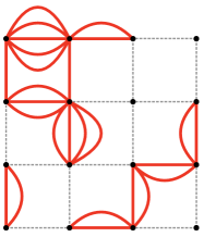
(a)

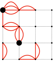
(b)

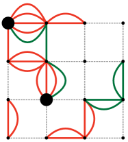
(c)

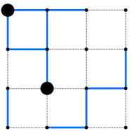
(d)

Figure 2: Current representation of the Ising model on $\mathbb{Z}^{2}$. (a) A current configuration $n:E\to\mathbb{N}$ contributing to the partition function $Z^{\text{Is}}$. (b) A current configuration contributing to the unnormalized correlation function $Z^{\text{Is}}\langle\tau_{0}\tau_{R}\rangle^{\text{Is}}$ where the large dots denote the lattice sites $0,R$. (c). A double current representation, where the red and green lines representation distinct configurations $n_{1},n_{2}$ contributing to the unnormalized correlation function $(Z^{\text{Is}}\langle\tau_{0}\tau_{R}\rangle^{\text{Is}})^{2}$. The large dots denote the lattice sites $0,R$. (d). A double current representation, where only the trace $\hat{n}$ (compared to Fig. 2c) is shown.

Consider the standard Ising model on a finite graph $G$,

$$H^{\text{Is}}(\tau)=-\sum_{e=ij}\tau_{i}\tau_{j}$$ (24)

So that the partition function is given by

$$Z^{\text{Is}}=\sum_{\tau}\prod_{e=ij}e^{\beta\tau_{i}\tau_{j}}$$ (25)

For each edge $e=ij$, we can expand the Boltzmann weight $e^{\beta\tau_{i}\tau_{J}}$ via Taylor series. This introduces an extra $\mathbb{N}$ degree of freedom on each edge $e$ corresponding to the order of the Taylor series expansion, and thus a current configuration on the edges $n:E\to\mathbb{N}$ [29]. Integrating over all spin configurations $\tau$ induces an interaction between the currents on distinct edges. More specifically, we have

$$Z^{\text{Is}}=\sum_{n}\frac{\beta^{n}}{n!}\times 1\{\partial n=\emptyset\}$$ (26)

Where $\beta^{n}\equiv\prod_{e}\beta^{n_{e}}$ and $n!\equiv\prod_{e}n_{e}!$. Note that $\partial n$ denote the endpoints of the current configuration $n$, that is, the set of vertices $i$ with an odd parity of neighboring edges in $n$, i.e., $\delta_{i}n=\sum_{e\sim i}n_{e}$. A typical current configuration is shown in Fig. 2a. Due to the restriction that $\partial n=\emptyset$, we see that each vertex must be adjacent to an even (possibly 0) number of edges in $n$.

One can perform a similar expansion for the unnormalized correlation function

$$Z^{\text{Is}}\langle\tau_{0}\tau_{R}\rangle^{\text{Is}}=\sum_{n}\frac{\beta^{n}}{n!}\times 1\{\partial n=0,R\}$$ (27)

Where the only difference is that the summation only includes current configurations with endpoints at lattice sites $0,R$ (see Fig. 2b for a typical configuration).

Notice that the partition function and unnormalized correlation functions are written over different sums of current configurations, and thus cannot define a probability distribution. Mathematicians have realized that one can circumvent this problem by applying a double current representation [29, 40]: create two identical copies of the same Hamiltonian so that one can compute the square of the unnormalized correlation functions, i.e.,

$$(Z^{\text{Is}}\langle\tau_{0}\tau_{R}\rangle^{\text{Is}})^{2}=\sum_{n_{1},n_{2}}\prod_{i=1}^{2}\frac{\beta^{n_{i}}}{n_{i}!}1\{\partial n_{i}=0,R\}$$ (28)

The key observation is to note that while each (duplicated) current configuration $n_{1},n_{2}$ must have endpoints at lattice site $0,R$, their sum $n\equiv n_{1}+n_{2}$ does not have any endpoints, as shown in Fig. 2c. The switching lemma [29, 38] formalizes this intuition so that one can rewrite

$$(Z^{\text{Is}}\langle\tau_{0}\tau_{R}\rangle^{\text{Is}})^{2} =\sum_{n_{1},n_{2}}1\{0\underset{n_{1}+n_{2}}{\leftrightarrow}R\}(\mu^{\text{Is}})^{\otimes 2}[n_{1},n_{2}]$$ (29)

$$(\mu^{\text{Is}})^{\otimes 2}[n_{1},n_{2}] =\prod_{i=1}^{2}\frac{\beta^{n_{i}}}{n_{i}!}1\{\partial n_{i}=\emptyset\}$$ (30)

Where $\{0\leftrightarrow_{n_{1}+n_{2}}R\}$ denotes the percolation event where lattice sites $0,R$ are connected in a cluster of $n_{1}+n_{2}$. Since the partition functions $(Z^{\text{Is}})^{2}$ is the normalization factor of the weights $(\mu^{\text{Is}})^{\otimes 2}[n_{1},n_{2}]$, we find that the correlation function can be written as the probability of a percolation event, i.e.,

$$(\langle\tau_{0}\tau_{R}\rangle^{\text{Is}})^{2} =(\mathbb{P}^{\text{Is}})^{\otimes 2}[0\underset{n_{1}+n_{2}}{\leftrightarrow}R]$$ (31)

$$(\mathbb{P}^{\text{Is}})^{\otimes 2}[n_{1},n_{2}] =\frac{(\mu^{\text{Is}})^{\otimes 2}[n_{1},n_{2}]}{(Z^{\text{Is}})^{2}}$$ (32)

We emphasize that the percolation event $\{0\leftrightarrow_{n_{1}+n_{2}}R\}$ is only dependent on the sum $n\equiv n_{1}+n_{2}$ of the two individual configurations; in fact, it only depends on the trace, which is a subgraph $\hat{n}:E\to\{0,1\}$ defined by including an edge $e$ in $\hat{n}$ if $n_{e}>0$, i.e., $\hat{n}=1\{n>0\}$. Therefore, we simplify our notation and write

$$(\langle\tau_{0}\tau_{R}\rangle^{\text{Is}})^{2}=(\mathbb{P}^{\text{Is}})^{\otimes 2}[0\leftrightarrow_{\hat{n}}R]$$ (33)

IV.2 A short review of the XY model

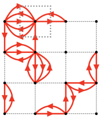
(a)

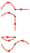
(b)

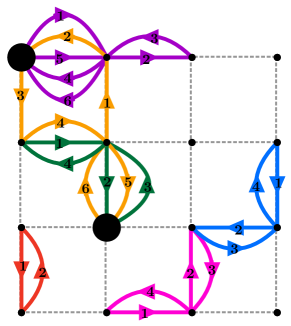
(c)

Figure 3: Current representation of the XY model on $\mathbb{Z}^{2}$. (a). A directed current configuration $\bm{\mathrm{n}}$ contributing to the partition function, i.e., with zero flow $\delta\bm{\mathrm{n}}=0$. (b). A possible pairing of incoming and outgoing edges of the boxed vertex in Fig. 3a. (c). A possible cyclic decomposition $\bm{\mathcal{C}}$ of the direct current $\bm{\mathrm{n}}$ in Fig. 3a. Distinct colors denote distinct loops and the numbers denote the ordering, e.g., $1\to 2\to 3\to 4\to 5\to 6\to 1$ for the orange cycle. Large black dots denote lattice site $0,R$.

Similar to the Ising model in the previous subsection, we can write the correlation functions of the standard XY model as percolation events in corresponding current representation. Here, we shall outline the main argument and refer the reader to Ref. [42] for details (see Appendix (C) for its application to the $U(1)\times\mathbb{Z}_{2}$ Hamiltonian). Consider the standard XY model on a finite graph $G$,

$$H^{\text{XY}}=-\sum_{e=ij}\sigma_{i}\cdot\sigma_{j}=-\frac{1}{2}\sum_{\bm{\mathrm{e}}=i\to j}\bar{\sigma}_{i}\sigma_{j}$$ (34)

Where $\sigma_{i}=e^{i\theta_{i}}\in\mathbb{S}^{1}\cong\mathbb{C}$. Notice that in contrast to the Ising model, the summation is over directed edges $\bm{\mathrm{e}}\in\bm{\mathrm{E}}$ and thus when computing the partition function $Z^{\text{XY}}$, the induced current is a directed configuration, i.e., $\bm{\mathrm{n}}:\bm{\mathrm{E}}\to\mathbb{N}$ and

$$Z^{\text{XY}}=\sum_{\bm{\mathrm{n}}}\cdots\times 1\{\delta\bm{\mathrm{n}}=0\}$$ (35)

Where we have omitted the corresponding weights $\cdots$ and chosen to focus on the interaction term induced by integrating over all XY spins. More concretely, $\delta_{i}\bm{\mathrm{n}}$ is the flow of the current out of the lattice site $i$, defined by $\delta_{i}\bm{\mathrm{n}}=\sum_{j\sim i}(\bm{\mathrm{n}}_{i\to j}-\bm{\mathrm{n}}_{j\to i})$ so that the condition $\delta\bm{\mathrm{n}}=0$ requires $\delta_{i}\bm{\mathrm{n}}=0$ at all lattice sites $i$. A typical directed configuration satisfying this condition is shown in Fig. 3a.

It would then appear that we can repeat the procedure outlined for the Ising model and write the correlation functions as a percolation event of the direct currents $\bm{\mathrm{n}}$. However, as first noticed by Ref. [42], a further degree of freedom is required. As shown in Fig. 3a, the zero flow requirement implies that we can decompose the directed current configuration into distinct cycles. More concretely, as shown in Fig. 3b (which corresponds to the boxed vertex in Fig. 2a), we can pair up the incoming- and outgoing-edges in any manner. By performing this decomposition at each vertex, we obtain a collection of directed cycles $\bm{\mathcal{C}}$. A typical configuration of $\bm{\mathcal{C}}$ is shown in Fig. 3c, where each distinct color denotes a distinct directed loop and the numbers specify the ordering, e.g., $1\to 2\to 3\to 4\to 5\to 6\to 1$ for the orange cycle.

By using an analogue of the switching lemma [29, 38] for the Ising model, the following correspondence was established

$$\langle\cos 2(\theta_{0}-\theta_{R})\rangle^{\text{XY}}\cong\mathbb{P}^{\text{XY}}[0\leftrightarrow_{\mathcal{C}}R]$$ (36)

Where $\cong$ denotes that the ratio of the two values are bounded above and below by constants, and $\{0\leftrightarrow_{\mathcal{C}}R\}$ denotes the percolation event in which there exists a directed loop in the collection $\bm{\mathcal{C}}$ which connects lattice sites $0,R$ (e.g., orange cycle in Fig. 3c). Similar to the Ising model, we emphasize that the percolation event $\{0\leftrightarrow_{\mathcal{C}}R\}$ is independent of the direction of each cycle in $\bm{\mathcal{C}}$ and thus warrants the notation $\mathcal{C}$ instead of $\bm{\mathcal{C}}$.

IV.3 Main result of $U(1)\times\mathbb{Z}_{2}$ Model

Similar to the cluster representation, the correlation-percolation correspondence in the current representation extends to the $U(1)\times\mathbb{Z}_{2}$ model and that the difficulty lies in finding the relation between two percolation event so that

Theorem 2 (see Appendix (C)).

Let the $U(1)\times\mathbb{Z}_{2}$ Hamiltonian $H$ in Eq. (1) be defined on a finite graph $G$. Then for any temperature,

$$\langle\cos 2(\theta_{0}-\theta_{R})\rangle_{G,\beta}\leq\langle\tau_{0}\tau_{R}\rangle_{G,\beta}$$ (37)

Sketch of Proof.

If we repeat the procedure for the standard XY models and define directed cyclic decomposition $\bm{\mathcal{C}}$, we see that the $U(1)$ correlations are related to the percolation events $\{0\leftrightarrow_{\mathcal{C}}R\}$. Since every directed cyclic decomposition corresponds to a directed current, i.e., $\bm{\mathcal{C}}\to\bm{\mathrm{n}}$, and each directed current corresponds to an undirected current, i.e., $\bm{\mathrm{n}}\to n$ (remove the directions), we see that we can also establish a correspondence between the $\mathbb{Z}_{2}$ correlations and the percolation event $\{0\leftrightarrow_{\hat{n}}R\}$. It’s then clear that if $\bm{\mathcal{C}}$ percolates between lattice sites $0,R$, then its induced undirected current configuration $n$ must also percolate, i.e.,

$$\{0\leftrightarrow_{\mathcal{C}}R\} \subseteq\{0\leftrightarrow_{\hat{n}}R\}$$ (38)

$$\mathbb{P}[0\leftrightarrow_{\mathcal{C}}R] \leq\mathbb{P}[0\leftrightarrow_{\hat{n}}R]$$ (39)

The statement then follows. ∎

One natural question that may arise is why not compare the conventional $U(1)$ correlations $\langle\cos(\theta_{0}-\theta_{R})\rangle$ with the $\mathbb{Z}_{2}$ correlations $\langle\tau_{0}\tau_{R}\rangle$ since, schematically, both require a double current representation. In short, the $U(1)\times\mathbb{Z}_{2}$ model is (heuristically) “already” a double current representation, since it is physically motivated by identical layers (e.g., twisted bilayer BSCCO). More concretely, note that in the standard Ising model, the correlations are obtained by considering two identical copies of the same Hamiltonian, i.e.,

$$H^{\text{Is}}(\sigma)+H^{\text{Is}}(\tau)=-\sum_{e=ij}(1+(\tau_{i}\sigma_{i})(\tau_{j}\sigma_{j}))\sigma_{i}\sigma_{j}$$ (40)

Where we need to sum over all Ising spin configuration $(\sigma,\tau)$. Note, however, that $(\sigma,\tau)\mapsto(\sigma,\tau\sigma)$ (where $\tau\sigma$ denotes site-wise multiplication), is a bijective mapping between spin configurations, and thus the duplicated Ising Hamiltonian is equivalent to

$$-\sum_{e=ij}(1+\tau_{i}\tau_{j})\sigma_{i}\sigma_{j}$$ (41)

This has the same form as the $U(1)\times\mathbb{Z}_{2}$ Hamiltonian in Eq. (1) with constant $\kappa_{e}=1$, except that the $U(1)$ spins in the latter are replaced by the simpler $\mathbb{Z}_{2}$ spins, i.e., $U(1)\mapsto\mathbb{Z}_{2}$. Therefore, heuristically, the $U(1)\times\mathbb{Z}_{2}$ model is “already” duplicated with respect to the Ising spins $\tau$.

V Comparison and Implications

V.1 Absence of Floating Phase on any Lattice - Rigorous

The main results in Theorem (1) and (2), proven using the distinct methods of cluster and current representation, are slightly different, i.e., the latter provides a slightly tighter bound. In any case, we see that if the $\mathbb{Z}_{2}$ Ising spins are disordered (exponentially decaying with respect to $R$) at some temperature $T$, then so must the $U(1)$ XY spins, and thus there cannot be a floating phase, i.e.,

$$T_{\text{TRSB}}\geq T_{c}$$ (42)

This guarantees the existence of a high $T_{c}$ TRSB superconductivity.

V.2 Suggestive Evidence of Absence of Vestigial Order

Apart from providing a stronger inequality over Theorem (1), the current representation in Theorem (2) also provides suggestive insight into why the converse may also hold (at least for the constant $\kappa_{e}=1$ scenario on a regular lattice such as $\mathbb{Z}^{d}$), i.e., the absence of vestigial order $T_{\text{TRSB}}\leq T_{c}$, as suggested by mean-field theory [1, 8] and numerics [22, 2, 23]. More specifically, we have shown that

$$\langle\cos 2(\theta_{0}-\theta_{R})\rangle\cong\mathbb{P}[0\leftrightarrow_{\mathcal{C}}R]$$ (43)

$$\langle\tau_{0}\tau_{R}\rangle\cong\mathbb{P}[0\leftrightarrow_{\hat{n}}R]$$ (44)

Where the cyclic decomposition $\bm{\mathcal{C}}$ induces the undirected current $n$ as argued previously, i.e., $\bm{\mathcal{C}}\to\bm{\mathrm{n}}\to n$. It is thus worth mentioning that the constructed current representation $\mathbb{P}$ for the $U(1)\times\mathbb{Z}_{2}$ Hamiltonian with constant $\kappa_{e}=1$ is related to that of the standard XY model $\mathbb{P}^{\text{XY}}$ via the following relation

$$\mathbb{P}[\bm{\mathcal{C}}]\propto 2^{C(\hat{n})}\mathbb{P}^{\text{XY}}[\bm{\mathcal{C}}]$$ (45)

Where $C(\hat{n})$ denote the number of clusters in the induced trace $\hat{n}$ (e.g., $C(\hat{n})=6$ in the example of Fig. 2d, where isolated vertices are also counted). Note the two percolation events $\{0\leftrightarrow_{\mathcal{C}}R\}$ and $\{0\leftrightarrow_{\hat{n}}R\}$ also occur in the standard XY model. However, since it’s well-known that the standard XY model only has a single phase transition on $\mathbb{Z}^{d}$, the two percolation events are expected to coincide in the XY model. The extra factor $2^{C(\hat{n})}$ is not expected to change this behavior, though it may change the critical temperature.

V.3 Extension to Finite Coupling Strength $J_{2}<\infty$

Based on the previous two discussions, it would seem that the current representation is always better than the cluster representation, since the former provides (slightly) stronger statements and better insights. However, we argue that the cluster representation may possibly have its own virtues. Mathematically, it is well known that the cluster representation satisfies the FKG condition [43, 29], which has been extensively used to provide elegant statements regarding the standard Ising [31, 30, 29] and XY model [36]. The corresponding current representation, however, is known to not possess such a quality. This begs the question as to whether the cluster representation for the $U(1)\times\mathbb{Z}_{2}$ model possesses similar attributes.

More physically relevant, though, is that the cluster representation can be easily extended to the finite coupling $J_{2}<\infty$ system to establish a correlation-percolation correspondence analogous to Eq. (11). However, the difficulty there is that the relation between the percolation events corresponding to the $U(1)$ and $\mathbb{Z}_{2}$ transition is less clear, i.e., the analogous $p^{\sigma}_{e}\geq p_{e}^{\tau}$ used in Theorem (1) is no longer true. This is to be expected, since the edge (conditional) probabilities $p_{e}$ only depend on the edge weights $w_{e}$ of the spin configurations and not the priori distribution of each $\sigma_{i}$ (i.e., what if we integrate over a non-uniform distribution of $\sigma_{i}\in\mathbb{S}^{1}$, which occurs, for example, in the presence of a magnetic field). For example, suppose that the probability distribution of spin configurations (analogous to Eq. (5)) is schematically written as

$$\mathbb{P}[\sigma]\propto\prod_{e=ij}w_{e}(\sigma)\prod_{i}\nu_{i}(\sigma)$$ (46)

Where $w_{e}(\sigma)$ depends on $\sigma$ implicitly through the values of $\sigma_{i},\sigma_{j}$, and $\nu_{i}(\sigma)$ depends on $\sigma$ implicitly through its value $\sigma_{i}$ on lattice site $i$ ($\nu_{i}(\sigma)=1$ in the standard Ising or XY models). In this case, the corresponding edge probabilities $p_{e}$ will be independent of $\nu_{i}$. In the finite coupling strength system in Eq. (2), the Josephson tunneling acts as a priori distribution $\nu_{i}$ and thus is not detected on the level of conditional probability $\sim\mathbb{P}[\omega|\sigma]$; rather, one must consider the joint distribution $\sim\mathbb{P}[(\omega,\sigma)]$, which is much more difficult.

V.4 Insights towards Order of Criticality

Another interesting question is the nature (first order or higher) of the transition, provided that the conjectured single phase transition exists, i.e., $T_{\text{TRSB}}=T_{c}$. Indeed, from mean-field theory [1, 8], we know that the transition is of second order for all $J_{2}>0$ (and not just the strong coupling limit $J_{2}\to\infty$) and thus should hold true for $d\geq 4$ dimensions in $\mathbb{Z}^{d}$. In Ref. [2], the authors numerically found that the transition is first order in $d=3$ dimensions (regardless of the coupling strength), and thus brings into question whether there is a change in behavior between $d=3,4$ dimensions. Although we do not have a definitive answer for this question, the following discussion may prove insightful.

Consider $d=2$ dimensions. For the standard XY model, it is usually argued that the transition is continuous (higher than first order) due to the absence of spontaneous symmetry breaking by Mermin-Wagner. For the $U(1)\times\mathbb{Z}_{2}$ Hamiltonian with $\kappa_{e}=1$, recent 2D numerical results suggest that the $U(1)$ correlations undergo a BKT phase transition [22], and thus one would can argue that $U(1)$ correlation length diverges as $T\searrow T_{c}$. If so, the inequalities in Theorem (1) and (2) would imply that the $\mathbb{Z}_{2}$ correlation length also diverges (again assuming that $T_{c}=T_{\text{TRSB}}$). Hence, the conjectured single phase transition is presumably continuous in $d=2$ dimensions. With that in mind, the transition is continuous in $d=2$ and $d\geq 4$ dimension, what reason could cause the transition to become discontinuous in $d=3$ dimensions?

Admittedly, the previous argument is not definitive, and one may attempt to circumvent it. For example, Mermin-Wagner by itself does not imply that the transition is BKT or continuous. Indeed, in Ref. [48, 49, 50], the authors constructed a counter example in which the system has a continuous symmetry (thus obeying Mermin-Wagner) and yet exhibited long-range order in $d=2$ dimension, i.e., even though the magnetization is $=0$, the spin-spin correlation functions do not decay to zero. More specifically, they proved that the counterexample exhibited a first order phase transition in $d=2$. However, we argue the above counter example does not apply to our system:

1. The constructed example is quite unphysical since they require to take a parameter $p\to\infty$, in which the phase transition changes from being higher order at $p=1$ to first order as $p\to\infty$. In comparison, although our model corresponds to the strong coupling limit $J_{2}\to\infty$, it has been consistently shown (in 2D [22] and 3D [23, 2]) that the transition is qualitatively independent of the coupling strength.

2. 2D numerics [22] suggest that at arbitrary finite coupling $J_{2}>0$ (though they did not go to the strong coupling limit), the $U(1)$ spin-spin correlations decay algebraically below the critical temperature and thus exhibit a BKT transition. This is in contrast to the counter example constructed in Ref. [48, 49, 50].

VI Simplified Models

So far, we have shown that the system in Eq. (1) cannot have a floating phase, i.e., must satisfy $T_{\text{TRSB}}\geq T_{c}$ on any lattice. The converse inequality (absence of vestigial order) $T_{\text{TRSB}}\leq T_{c}$, however is much more difficult for the $U(1)\times\mathbb{Z}_{2}$ model. Therefore, in this section, we will attempt to provide insight by studying two simplified models, i.e., replacing the $U(1)$ degree of freedom $\sigma$ in Eq. (1) with $\mathbb{Z}_{4}$ and $\mathbb{Z}_{2}$ clock models. In fact, with this simplification, we are capable of studying a larger class of $U(1)\times\mathbb{Z}_{2}$ Hamiltonian, i.e., before simplification,

$$H_{\rho}(\sigma,\tau)=-\sum_{e=ij}\kappa_{e}(\rho_{+}+\rho_{-}\tau_{i}\tau_{j})\sigma_{i}\cdot\sigma_{j}$$ (47)

Where $\rho\in[0,1]$ and $\rho_{\pm}=1\pm\rho$. Note that $\rho=0$ corresponds to the Hamiltonian in Eq. (1). The simplifications $U(1)\mapsto\mathbb{Z}_{2},\mathbb{Z}_{4}$ can then be regarded as adding an arbitrary interaction $-\lambda_{2}\sum_{i}\cos(2\theta_{i})$ and $-\lambda_{4}\sum_{i}\cos(4\theta_{i})$ and taking the limit $\lambda_{2},\lambda_{4}\to\infty$, respectively.

Similar to Eq. (1), the larger class $H_{\rho}$ with constant $\kappa_{e}=1$ can be mapped to the strong coupling limit of twisted bilayer BSCCO and frustrated $n\geq 3$-band superconductors. Indeed, the latter was derived in Eq. (8) of Ref. [2]. The former corresponds to the case where there is nonzero 1^st order Josephson coupling $J_{1}$ between the two layers, i.e., in addition to Eq. (2), we have

$$H_{J_{1},J_{2}}(\phi^{\pm})=H_{J_{2}}(\phi^{\pm})-J_{1}\sum_{i}\cos\phi_{i}$$ (48)

In this case, $H_{\rho}$ corresponds to the Hamiltonian $H_{J_{1},J_{2}}$ with $\rho=J_{1}/4J_{2}$ kept fixed while we take $J_{2}\to\infty$.

Due to the correspondence, it is conjectured that the two transitions $T_{c},T_{\text{TRSB}}$ coincide at $\rho=0$ and split for $\rho\neq 0$, i.e., $T_{\text{TRSB}}<T_{c}$. Indeed, an exact understanding of $H_{J_{1},J_{2}}$ is known within the context of mean-field theory [8] without the need for simplifications. Therefore, the simplifications $U(1)\mapsto\mathbb{Z}_{4},\mathbb{Z}_{2}$ are to probe the behavior of the system in low dimensions (though we will prove the statements for any lattice).

VI.1 $U(1)\mapsto\mathbb{Z}_{2}$

Consider the simplification

$$H_{\rho}^{\mathbb{Z}_{2}}(\sigma,\tau)=-\sum_{e=ij}\kappa_{e}(\rho_{+}+\rho_{-}\tau_{i}\tau_{j})\sigma_{i}\sigma_{j}$$ (49)

Where $\sigma_{i}=\pm 1$. Since $(\sigma,\tau)\mapsto(\sigma,\tau\sigma)$ (where $\tau\sigma$ denotes site-wise multiplication) is a bijective mapping between spin configurations, we see that $H_{\rho}^{\mathbb{Z}_{2}}$ is equivalent to decoupled Ising models, and thus we have the following statement.

Theorem 3 (see Appendix (D)).

Let $G$ be any finite graph, and $\langle\cdots\rangle^{\mathrm{Is}}_{\beta}$ denotes the thermal average with respect to the Ising model (with $s_{i}=\pm 1$) on $G$ with edge-coupling $\kappa_{e}$ and inverse temperature $\beta$. Then

$$\langle\sigma_{0}\sigma_{R}\rangle_{\rho,\beta}^{\mathbb{Z}_{2}} =\langle s_{0}s_{R}\rangle^{\mathrm{Is}}_{\beta\rho_{+}}$$ (50)

$$\langle\tau_{0}\tau_{R}\rangle_{\rho,\beta}^{\mathbb{Z}_{2}} =\langle s_{0}s_{R}\rangle^{\mathrm{Is}}_{\beta\rho_{+}}\langle s_{0}s_{R}\rangle^{\mathrm{Is}}_{\beta\rho_{-}}$$ (51)

The previous correspondence then implies that

$$``T_{c}"=\rho_{+}T^{\mathrm{Is}}_{c}\quad\geq\quad T_{\text{TRSB}}=\rho_{-}T^{\mathrm{Is}}_{c}$$ (52)

Where equality only holds at $\rho=0$. Here, $T_{c}^{\text{Is}}$ is the critical temperature of the corresponding Ising model and we write $``T_{c}"$ since the original $U(1)$ spins are replaced by $\mathbb{Z}_{2}$ spins.

VI.2 $U(1)\mapsto\mathbb{Z}_{4}$

Note that the previous simplification $U(1)\mapsto\mathbb{Z}_{2}$ was trivial in the sense that the system is can be exactly mapped to decoupled Ising models. In this section, we shall consider the slightly more general case where $U(1)\mapsto\mathbb{Z}_{4}$, i.e., $\sigma_{i}=(1,0),(0,1),(-1,0),(0,-1)$ at each lattice site $i$. It should be noted that the $\mathbb{Z}_{4}$ clock model is special in the sense that the $(X,Y)$ degree of freedom can be replaced by 2 independent Ising degrees of freedom, i.e., $\xi,\eta=X\pm Y$. Therefore, the Hamiltonian can be rewritten as

$$H^{\mathbb{Z}_{4}}_{\rho}=-\frac{1}{2}\sum_{e=ij}\kappa_{e}(\rho_{+}+\rho_{-}\tau_{i}\tau_{j})(\xi_{i}\xi_{j}+\eta_{i}\eta_{j})$$ (53)

To simplify notation, let $\langle\psi\rangle$ be shorthand for the correlation $\langle\psi_{0}\psi_{R}\rangle^{\mathbb{Z}_{4}}_{\rho,\beta}$ where $\psi$ can be any of the 7 options $\psi=\tau,\xi,\eta,\tau\xi,\tau\eta,\xi\eta,\tau\xi\eta$, each of which can (in principle) define a separate transition temperature $T_{\psi}$. However, using the symmetries of the Hamiltonian in Eq. (53) and the corresponding FKG inequalities [21, 29, 27], the following (in)equalities can be shown.

Theorem 4.

For any $0\leq\rho\leq 1$,

$$\langle\xi\rangle =\langle\eta\rangle,\quad\langle\tau\xi\rangle=\langle\tau\eta\rangle$$ (54)

$$\langle\tau\rangle =\langle\tau\xi\eta\rangle\geq\langle\tau\xi\rangle\langle\xi\rangle$$ (55)

$$\langle\xi\rangle \geq\langle\tau\xi\rangle\geq\langle\tau\rangle\langle\xi\rangle$$ (56)

$$\langle\xi\rangle \geq\langle\xi\eta\rangle\geq\langle\xi\rangle^{2}$$ (57)

Moreover,

$$\langle\xi\eta\rangle\geq\langle\tau\rangle$$ (58)

Where equality holds if $\rho=0$.

Proof.

From the Hamiltonian in Eq. (53), it’s clear that $\langle\xi\rangle=\langle\eta\rangle$ and $\langle\tau\xi\rangle=\langle\tau\eta\rangle$ due to the symmetry $\xi\leftrightarrow\eta$. Also notice that when summing over the configuration $(\tau,\xi,\eta)$, the mapping $\tau\mapsto\tau\xi\eta$ is a bijective transformation which keeps the Hamiltonian invariant. Therefore, $\langle\tau\rangle=\langle\tau\xi\eta\rangle$. By Ginibre’s/FKG inequality (Prop 3, 5 and Example 4 of Ref. [27]), we see that

$$\langle\tau\xi\eta\rangle \geq\langle\tau\xi\rangle\langle\eta\rangle=\langle\tau\xi\rangle\langle\xi\rangle$$ (59)

$$\langle\tau\xi\rangle \geq\langle\tau\rangle\langle\xi\rangle$$ (60)

$$\langle\xi\eta\rangle \geq\langle\xi\rangle\langle\eta\rangle=\langle\xi\rangle^{2}$$ (61)

It should be noted that the conditional expectation $\langle\xi\rangle^{\tau}$ (i.e., computing the thermal average of $\xi_{0}\xi_{R}$ if the $\mathbb{Z}_{2}$ configuration $\tau$ were fixed) is equal to that of an Ising model $-\sum_{e}\kappa_{e}^{\prime}\xi_{i}\xi_{j}$ with edge coupling

$$\kappa_{e}^{\prime}=\frac{1}{2}\kappa_{e}(\rho_{+}+\rho_{-}\tau_{i}\tau_{j})\geq 0,\quad e=ij$$ (62)

Therefore, by Griffiths 1^st inequality [27, 21, 29], we see that $\langle\xi\rangle^{\tau}=\langle\xi\rangle^{\mathrm{Is}^{\prime}}\geq 0$, and thus

$$\langle\tau\xi\rangle=\langle\tau\langle\xi\rangle^{\tau}\rangle\leq\langle\langle\xi\rangle^{\tau}\rangle=\langle\xi\rangle$$ (63)

Where the first equality can be understood as first averaging over $\xi,\eta$, then averaging over $\tau$. The inequality uses the trivial fact $\tau_{0}\tau_{R}\leq 1$. Similarly, we have

$$\langle\xi\eta\rangle=\langle\xi\langle\eta\rangle^{\xi,\tau}\rangle\leq\langle\langle\eta\rangle^{\xi,\tau}\rangle=\langle\eta\rangle=\langle\xi\rangle$$ (64)

Where $\langle\eta\rangle^{\xi,\tau}$ is the conditional expectation with respect to fixing $\xi,\tau$.

For the last inequality, note that $\langle\tau\rangle=\langle\tau\xi\eta\rangle$ and as before, the conditional expectation $\langle\xi\eta\rangle^{\tau}=\langle\xi\rangle^{\mathrm{Is}^{\prime}}\langle\eta\rangle^{\mathrm{Is}^{\prime}}$ (fixing the $\mathbb{Z}_{2}$ spin configuration $\tau$) is equal to two independent Ising models with edge couplings $\kappa_{e}^{\prime}$. Therefore, by Griffiths 1st inequality [27, 21, 29], we see that $\langle\xi\rangle^{\mathrm{Is}^{\prime}},\langle\eta\rangle^{\mathrm{Is}^{\prime}}\geq 0$ and thus

$$\langle\tau\rangle =\langle\tau\xi\eta\rangle$$ (65)

$$=\langle\tau\langle\xi\eta\rangle^{\tau}\rangle$$ (66)

$$\leq\langle\langle\xi\eta\rangle^{\tau}\rangle,\quad\tau_{0}\tau_{R}\leq 1$$ (67)

$$=\langle\xi\eta\rangle$$ (68)

In the case where $\rho=0$, we see that $\tau\leftrightarrow\xi\eta$ is a bijective transform which leaves the Hamiltonian invariant and thus we obtain equality,

$$\langle\tau\rangle=\langle\xi\eta\rangle$$ (69)

∎

Using the inequalities, it’s straightforward to check that $T_{\text{TRSB}}\equiv T_{\tau}$ and $``T_{c}"\equiv T_{\xi\eta}$ are the only (possibly) independent transition temperatures, i.e.,

$$T_{\xi} =T_{\eta}=T_{\xi\eta}$$ (70)

$$T_{\tau} =T_{\tau\xi\eta}$$ (71)

$$T_{\tau\xi} =T_{\tau\eta}=\min(T_{\tau},T_{\xi\eta})$$ (72)

Moreover, the last inequality implies that

$$T_{\text{TRSB}}\leq``T_{c}"$$ (73)

Where equality holds at $\rho=0$. Hence, we see that the system cannot exhibit vestigial order on any lattice despite having short-range interactions (in comparison to claims of Ref. [24]); at most, the two transitions coincide at the critical point $\rho=0$.

VII Summary and Discussion

As discussed in the main text (especially Sec. (V)), we have rigorously proven that the $U(1)\times\mathbb{Z}_{2}$ Hamiltonian in Eq. (1) does not exhibit a floating phase on any lattice structure, i.e., $T_{\text{TRSB}}\geq T_{c}$ (which includes the boundary cases where the transition temperature is possibly $=0,\infty$). The model is physically motivated by the either twisted bilayer BSCCO with only 2^nd order inter-layer Josephson coupling $J_{2}$ or $n\geq 3$-band superconductors with frustrated 1^st order inter-band Josephson coupling. In fact, it corresponds to the strong coupling limit (e.g., $J_{2}\to\infty$) of the previous models, which we have shown to be continuously connected to finite but large $J_{2}$ values [26]. From numerical simulations in 2D [22], 3D [23, 2] and exact mean-field understanding (for $d\geq 4$) [20, 1], it is believed that the qualitative properties of the systems are insensitive to the coupling strength and thus our result on the strong coupling limit sheds light onto the phase diagram. More concretely, it was conjectured that the two transitions coincide $T_{c}=T_{\text{TRSB}}$ for all coupling strength and dimensions. This is equivalent to both (1) the absence of a floating phase, $T_{\text{TRSB}}\geq T_{c}$ and (2) the absence of vestigial TRSB, $T_{\text{TRSB}}\leq T_{c}$. Therefore, the main result of this paper is that, at least in the strong coupling limit, property (1) holds true exactly on any lattice structure and thus guarantees the existence of high $T_{c}$ superconductivity with TRSB (and possibly high $T_{c}$ topological superconductivity [1]).

On the other hand, we do not definitively show whether property (2) holds true or not. However, if we were to make reasonable simplifications (as discussed in Sec. (VI) where we replace the $U(1)$ symmetry with $\mathbb{Z}_{4},\mathbb{Z}_{2}$ clock models), we can prove that the conjecture holds for the related $\mathbb{Z}_{4}\times\mathbb{Z}_{2}$ and $\mathbb{Z}_{2}\times\mathbb{Z}_{2}$ models on any lattice structure. In fact, the simplification permits us to study a larger class of Hamiltonians (which corresponds, for example, to the strong coupling limit of twisted bilayer BSCCO with arbitrary ratio of 1^st and 2^nd order Jospherson coupling $J_{1}/J_{2}$), and prove that the systems must satisfy property (2) on any lattice structure. This provides us a counter-example in which short-range interactions do not necessarily induce vestigial order and thus raises concerns for the claims of in Ref. [24].

Further implications (such as whether the conjectured single phase transition is of first or higher order, and possible extensions to finite coupling strengths) are also discussed in Sec. (V). However, since it is mostly suggestive evidence, we do not repeat them here.

VIII Acknowledegements

I am grateful for Steve A. Kivelson’s support and generosity during this project and also for providing extensive comments and suggestions on the draft. This work was supported, in part, by NSF Grant No. DMR-2000987 at Stanford University.

Appendix A Change of Variables

Lemma 5.

Let $f:\mathbb{S}^{1}\times\mathbb{S}^{1}\mapsto\mathbb{R}$ be bounded. Then

$$\int_{(-\pi,\pi)^{2}}\frac{d\phi_{+}}{2\pi}\frac{d\phi_{-}}{2\pi}f(\phi_{+},\phi_{-})=\int_{(-\pi,\pi)^{2}}\frac{d\theta}{2\pi}\frac{d\phi}{2\pi}f(\theta+\phi/2,\theta-\phi/2)$$ (74)

Where $\theta=(\phi_{+}+\phi_{-})/2$ is the average phase and $\phi=\phi_{+}-\phi_{-}$ is the phase difference.

Proof.

For simplicity, we will drop the normalization $1/2\pi$. Indeed, notice that

$$\int_{(-\pi,\pi)^{2}}d\phi_{\pm}f(\phi_{+},\phi_{-}) =\int_{-\pi}^{\pi}d\phi_{-}\int_{-\phi_{-}}^{2\pi-\phi_{-}}d\phi f(\phi_{-}+\phi,\phi_{-}),\quad\phi=\phi_{+}-\phi_{-}$$ (75)

$$=\int_{-\pi}^{\pi}d\phi_{-}\int_{-\pi_{-}}^{\pi-}d\phi f(\phi_{-}+\phi,\phi_{-})$$ (76)

$$=\int_{-\pi}^{\pi}d\phi\int_{-\pi}^{\pi}d\phi_{-}f(\phi_{-}+\phi,\phi_{-})$$ (77)

$$=\int_{-\pi}^{\pi}d\phi\int_{-\pi+\phi/2}^{\pi+\phi/2}d\theta f(\theta+\phi/2,\theta-\phi/2),\quad\theta=\phi_{-}+\phi/2$$ (78)

$$=\int_{(-\pi,\pi)^{2}}d\theta d\phi f(\theta+\phi/2,\theta-\phi/2)$$ (79)

Where the 2nd and 5th equality uses the fact that $\phi_{\pm}\mapsto f$ is $2\pi$-periodic, and thus the integration limits can be an arbitrarily chosen $2\pi$-interval. ∎

Appendix B (Random) Cluster Representation

In the main text, we have claimed that by choosing the edge probabilities $p_{e}^{\tau},p_{e}^{\sigma}$ appropriately and defining the subgraphs $\hat{\tau},\hat{\sigma}$, the $\mathbb{Z}_{2}$ and $U(1)$ spin-spin correlations can be mapped to percolation events. By comparing the edge probabilities $p_{e}^{\tau}\geq p_{e}^{\sigma}$, the ordering of percolation events (and thus correlations) becomes apparent. Therefore, in this section, we will follow Ref. [35] and prove our claim of correlation-percolation correspondence of the $U(1)\times\mathbb{Z}_{2}$ Hamiltonian in Eq. (1). As discussed in the main text, let $\mathbb{P}[\sigma,\tau]$ be the probability distribution of the spin configurations defined by the $U(1)\times\mathbb{Z}_{2}$ Hamiltonian in Eq. (1), i.e.,

$$\mathbb{P}[(\sigma,\tau)] \propto\prod_{e=ij}w_{e}(\sigma,\tau)$$ (80)

$$w_{e}(\sigma,\tau) =e^{\beta\kappa_{e}(1+\tau_{i}\tau_{j})\cos(\theta_{i}-\theta_{j})}$$ (81)

B.1 $\mathbb{Z}_{2}$ Correlations

Similar to that discussed in the main text for the standard Ising model (see Fig. 1), for a fixed spin configuration $(\sigma,\tau)$, define a random variable of subgraphs $\hat{\tau}:E\to\{0,1\}$ via the edge probability

$$p_{e}^{\tau}(\sigma,\tau) =\left[1-\frac{w_{e}(\sigma,\tau^{i})}{w_{e}(\sigma,\tau)}\right]1\{w_{e}(\sigma,\tau^{i})<w_{e}(\sigma,\tau)\}$$ (82)

$$=\left[1-e^{-2\beta\kappa_{e}\tau_{i}\tau_{j}\cos(\theta_{i}-\theta_{j})}\right]1\{\tau_{i}\tau_{j}\cos(\theta_{i}-\theta_{j})>0\}$$ (83)

So that

$$\mathbb{P}[\hat{\tau}|\sigma,\tau] =\prod_{e\in\hat{\tau}}p_{e}^{\tau}(\sigma,\tau)\prod_{e\notin\hat{\tau}}(1-p_{e}^{\tau}(\sigma,\tau))$$ (84)

$$\mathbb{P}[\hat{\tau},\sigma,\tau] =\mathbb{P}[\hat{\tau}|\sigma,\tau]\mathbb{P}[\sigma,\tau]$$ (85)

Theorem 6 (Cluster-Flip Invariance).

Let $\mathbb{P}_{G,\beta}$ be the probability distribution on $(\hat{\tau},\sigma,\tau)$ as befined previously on a finite graph $G$. Then $\mathbb{P}$ is invariant under cluster flips with respect to $\tau$, i.e.,

$$\mathbb{P}_{G,\beta}[(\hat{\tau},\sigma,\tau)]=\mathbb{P}_{G,\beta}[(\hat{\tau},\sigma,\tau^{C_{0}(\hat{\tau})})]$$ (86)

Where $C_{0}(\hat{\tau})$ is the cluster in $\hat{\tau}$ intersecting the lattice site $0$ and $\tau^{C_{0}(\hat{\tau})}$ denotes flipping the spins of $\tau$ only in $C_{0}(\hat{\tau})$. In particular, the $\mathbb{Z}_{2}$ correlation-percolation is established, i.e.,

$$\langle\tau_{0}\tau_{R}\rangle_{G,\beta}=\mathbb{P}_{G,\beta}[0\leftrightarrow_{\hat{\tau}}R]$$ (87)

Proof.

For notation simplicity, we shall omit the subscripts $G,\beta$. Notice that

$$\frac{\mathbb{P}[(\hat{\tau},\sigma,\tau^{C_{0}(\hat{\tau})})]}{\mathbb{P}[(\hat{\tau},\sigma,\tau)]} =\frac{\mathbb{P}[\hat{\tau}|\sigma,\tau^{C_{0}(\hat{\tau})}]}{\mathbb{P}[\hat{\tau}|\sigma,\tau]}\times\frac{\mathbb{P}[\sigma,\tau^{C_{0}(\hat{\tau})}]}{\mathbb{P}[\sigma,\tau]}$$ (88)

Note that the ratios only depends on edge $e$ on the boundary of $C_{0}(\hat{\tau})$ since $w_{e}(\sigma,\tau)$ is invariant if both endpoints are flipped, i.e., $\tau_{i},\tau_{j}\mapsto-\tau_{i}\tau_{j}$ where $e=ij$. More specifically,

$$\frac{\mathbb{P}[(\hat{\tau},\sigma,\tau^{C_{0}(\hat{\tau})})]}{\mathbb{P}[(\hat{\tau},\sigma,\tau)]} =\prod_{e=ij\in\partial C_{0}(\hat{\tau})\atop{i\in C_{0}(\hat{\tau}),j\notin C_{0}(\hat{\tau})}}\frac{p_{e}^{\tau}(\sigma,\tau^{i})w_{e}(\sigma,\tau^{i})}{p_{e}^{\tau}(\sigma,\tau)w_{e}(\sigma,\tau)}$$ (89)

By definition of $p_{e}^{\tau}$, it’s straightforward to check that each term in the product is $=1$. The statement then follows. ∎

B.2 $U(1)$ Correlations

The $U(1)$ correlation-percolation correspondence for the higher order term $\langle\cos 2(\theta_{0}-\theta_{R})\rangle$ is much more difficult to establish than $\mathbb{Z}_{2}$ correlation.; in fact, it relies on first establishing a correspondence for the conventional term $\langle\cos(\theta_{0}-\theta_{R})\rangle$. In this section, we shall follow Ref. [35] (with slight modifications) in establishing the correspondence for the $U(1)\times\mathbb{Z}_{2}$ model in Eq. (1). Similar to the $\mathbb{Z}_{2}$ subgraph $\hat{\tau}$, let $\hat{\xi}:E\to\{0,1\}$ be constructed with edge probability

$$p_{e}^{\xi}(\sigma,\tau) =\left[1-\frac{w_{e}(\sigma^{\xi,i},\tau)}{w_{e}(\sigma,\tau)}\right]1\{w_{e}(\sigma^{\xi,i},\tau)<w_{e}(\sigma,\tau)\}$$ (90)

$$=\left[1-e^{-4\beta\kappa_{e}\cos\theta_{i}\cos\theta_{j}}\right]1\{\tau_{i}\tau_{j}=\xi_{i}\xi_{j}=1\}$$ (91)

Where $\xi$ is the sign of the $x$ component of $\sigma$ ($\cos\theta$), and $\sigma^{\xi,i}$ denotes flipping the spin only at the lattice site $i$ along the $x$ direction, i.e., $\xi_{i}\mapsto-\xi_{i}$ or $\theta_{i}\mapsto\pi-\theta_{i}$. As before, this defines a probability distribution on $(\hat{\xi},\sigma,\tau)$. Similarly, define the subgraph $\hat{\sigma}^{\eta}:E\to\{0,1\}$ by using the sign $\eta=\pm 1$ of the $y$ component of $\sigma$ ($\sin\theta$), i.e., the edge probability is

$$p_{e}^{\eta}(\sigma,\tau)=\left[1-\frac{w_{e}(\sigma^{\eta,i},\tau)}{w_{e}(\sigma,\tau)}\right]1\{w_{e}(\sigma^{\eta,i},\tau)<w_{e}(\sigma,\tau)\}$$ (92)

And thus this defines a probability on $(\hat{\eta},\sigma,\tau)$.

As mentioned in the main text, to establish the correspondence for $\langle\cos 2(\theta_{0}-\theta_{R})\rangle$, we require both $\hat{\xi},\hat{\eta}$ and thus the first question is then whether we can define a joint probability on $(\hat{\xi},\hat{\eta},\sigma,\tau)$. Since each edge is independently established (conditional with respect to the fixed spin configuration $\sigma,\tau$), $\hat{\xi}_{e},\hat{\eta}_{e}$ are Bernoulli random variables and thus whether we can define a joint distribution depends on choosing the appropriate correlation $c_{e}(\sigma,\tau)$ so that the following values are $\geq 0$, i.e.,

$$\mathbb{P}[\hat{\xi}_{e}=1,\hat{\eta}_{e}=1|\sigma,\tau] =c_{e}$$ (93)

$$\mathbb{P}[\hat{\xi}_{e}=0,\hat{\eta}_{e}=1|\sigma,\tau] =p_{e}^{\eta}-c_{e}$$ (94)

$$\mathbb{P}[\hat{\xi}_{e}=1,\hat{\eta}_{e}=0|\sigma,\tau] =p_{e}^{\xi}-c_{e}$$ (95)

$$\mathbb{P}[\hat{\xi}_{e}=0,\hat{\eta}_{e}=0|\sigma,\tau] =1-p_{e}^{\xi}-p_{e}^{\eta}+c_{e}$$ (96)

Moreover, we wish to choose the correlation $c_{e}$ so that a analogous cluster-flip invariance property is satisfied. Hence, it turns out that we should choose the correlation $c_{e}=p_{e}^{\sigma}$ as defined in the proof of the main result, Theorem (1), i.e.,

$$p_{e}^{\sigma}(\sigma,\tau) =\left[1+\frac{w_{e}(\sigma^{\xi\eta,i},\tau)}{w_{e}(\sigma,\tau)}-\frac{w_{e}(\sigma^{\xi,i},\tau)}{w_{e}(\sigma,\tau)}-\frac{w_{e}(\sigma^{\eta,i},\tau)}{w_{e}(\sigma,\tau)}\right]\times 1\{w_{e}(\sigma^{\xi,i},\tau),w_{e}(\sigma^{\eta,i},\tau)<w_{e}(\sigma,\tau)\}$$ (97)

Indeed, let us verify that this choice of correlation satisfies the necessary properties.

Theorem 7 (Cluster-Flip Invariance).

Let $\mathbb{P}_{G,\beta}$ denote the joint probability on $(\hat{\xi},\hat{\eta},\sigma,\tau)$ on a finite graph $G$ defined previously. Then $\mathbb{P}_{G,\beta}$ is well-defined and satisfies the cluster-flip invariance with respect to $\xi,\eta$, i.e.,

$$\mathbb{P}_{G,\beta}[(\hat{\xi},\hat{\eta},\sigma,\tau)] =\mathbb{P}_{G,\beta}[(\hat{\xi},\hat{\eta},\sigma^{\xi,C_{0}(\hat{\xi})},\tau)]$$ (98)

$$\mathbb{P}_{G,\beta}[(\hat{\xi},\hat{\eta},\sigma,\tau)] =\mathbb{P}_{G,\beta}[(\hat{\xi},\hat{\eta},\sigma^{\eta,C_{0}(\hat{\eta})},\tau)]$$ (99)

Where $C_{0}(\hat{\xi})$ is the cluster in $\hat{\xi}$ intersecting the lattice site $0$ and $\sigma^{\xi,C_{0}(\hat{\xi})}$ denotes flipping the spin configuration $\sigma$ only at lattice sites within the cluster $C_{0}(\hat{\xi})$ along the $x$ component, i.e., $\xi_{i}\mapsto-\xi_{i}$ or $\theta_{i}\mapsto\pi-\theta_{i}$ for $i\in C_{0}(\hat{\xi})$. The notation is similar for $\xi\mapsto\eta$.

Proof.

The proof follows that given in Ref. [35], though we simplify/modify some parts to illuminate some of the situation. For the $U(1)\times\mathbb{Z}_{2}$ Hamiltonian in Eq. (1), the appropriate probability $p_{e}^{\sigma}$ happens to satisfy

$$p_{e}^{\sigma}=p_{e}^{\xi}\times p_{e}^{\eta}$$ (100)

And thus conditions (93)-(96) are easily seen to satisfy. For general weights $w_{e}$, this is not as simple [35]. Let us now show that the cluster flip invariance holds true along $\xi$. The proof is similarly applied to that along $\eta$. Notice that

$$\frac{\mathbb{P}[(\hat{\xi},\hat{\eta},\sigma,\tau^{C_{0}(\hat{\xi})})]}{\mathbb{P}[(\hat{\xi},\hat{\eta},\sigma,\tau)]} =\frac{\mathbb{P}[\hat{\xi},\hat{\eta}|\sigma^{\xi,C_{0}(\hat{\xi})},\tau]}{\mathbb{P}[\hat{\xi},\hat{\eta}|\sigma,\tau]}\times\frac{\mathbb{P}[\sigma^{\xi,C_{0}(\hat{\xi})},\tau]}{\mathbb{P}[\sigma,\tau]}$$ (101)

Similar to the proof in Theorem (6), we see that if an edge $e=ij$ has endpoints $i,j$ entirely in $C_{0}(\hat{\xi})$ or entirely outside of the cluster, then the edge weights $w_{e}(\sigma,\tau),w_{e}(\sigma^{\xi,i},\tau),w_{e}(\sigma^{\eta,i},\tau)$ and $w_{e}(\sigma^{\xi\eta,i},\tau)$ are all invariant under $\sigma\mapsto\sigma^{\xi,C_{0}(\hat{\xi})}$. Therefore, we only need to consider edges in the boundary of $C_{0}(\hat{\xi})$ so that $e=ij$ with $i\in C_{0}(\hat{\xi})$ and $j\notin C_{0}(\hat{\xi})$, i.e.,

$$\frac{\mathbb{P}[(\hat{\xi},\hat{\eta},\sigma,\tau^{C_{0}(\hat{\xi})})]}{\mathbb{P}[(\hat{\xi},\hat{\eta},\sigma,\tau)]} =\prod_{e=ij\in\partial C_{0}(\hat{\xi})\atop i\in C_{0}(\hat{\xi}),j\notin C_{0}(\hat{\xi})}\frac{\mathbb{P}[\hat{\xi}_{e}=0,\hat{\eta}_{e}|\sigma^{\xi,C_{0}(\hat{\xi})},\tau]}{\mathbb{P}[\hat{\xi}_{e}=0,\hat{\eta}_{e}|\sigma,\tau]}\frac{w_{e}(\sigma^{\xi,i},\tau)}{w_{e}(\sigma,\tau)}$$ (102)

Where we used the fact that since $e\in\partial C_{0}(\hat{\xi})$, it cannot be in $\hat{\xi}$ (the cluster $C_{0}(\hat{\xi})$ stops growing at its boundary). However, the value of $\hat{\eta}_{e}$ could be either $0$ or $1$ and thus we must consider all possible cases as described by Eqs. (94) and (96). More specifically, it is sufficient to prove that the following term

$$w_{e}(\sigma,\tau)\mathbb{P}[\hat{\xi}_{e}=0,\hat{\eta}_{e}|\sigma,\tau]$$ (103)

Is invariant under spin-flip $\sigma\mapsto\sigma^{\xi,i}$ where $i$ is an endpoint of the edge $e\in\partial C_{0}(\hat{\xi})$.

For notation simplicity, let me fix an edge $e=ij$ in the boundary for the remainder of this proof so that we can omit the subscript. We shall also write

$$w \equiv w_{e}(\sigma,\tau)$$ (104)

$$w^{\xi} \equiv w_{e}(\sigma^{\xi,i},\tau)$$ (105)

$$w^{\eta} \equiv w_{e}(\sigma^{\xi,i},\tau)$$ (106)

$$w^{\xi\eta} \equiv w_{e}(\sigma^{\xi\eta,i},\tau)$$ (107)

And similarly for $p^{\xi},p^{\eta},p^{\sigma}$ so that

$$wp^{\xi} =\left[w-w^{\xi}\right]1\{w^{\xi}<w\}$$ (108)

$$wp^{\eta} =\left[w-w^{\eta}\right]1\{w^{\eta}<w\}$$ (109)

$$wp^{\sigma} =\left[w+w^{\xi\eta}-w^{\xi}-w^{\eta}\right]1\{w^{\xi},w^{\eta}<w\}$$ (110)

In fact, it is more illuminating if we write the previous equations in the following form

$$w(1-p^{\xi}) =\min(w,w^{\xi})$$ (111)

$$w(1-p^{\eta}) =\min(w,w^{\eta})$$ (112)

Note that under spin-flip $\sigma\mapsto\sigma^{\xi,i}$ (where $i$ is one endpoint of the fixed edge $e$), we have

$$w,w^{\xi},w^{\eta},w^{\xi\eta} \mapsto w^{\xi},w,w^{\xi\eta},w^{\eta}$$ (113)

And thus $w(1-p^{\xi})$ is invariant under the spin-flip. If we compare the 2 possible cases (corresponding to $\hat{\eta}=1,0$) in Eq. (94) and (96), we see that they differ by the invariant variable $w(1-p^{\xi})$ and thus we only need to consider one of the two cases, say that corresponding to Eq. (94), i.e.,

$$w(p^{\eta}-p^{\sigma})=[w-w^{\eta}]1\{w^{\eta}<w<w^{\xi}\}+[w^{\xi}-w^{\xi\eta}]1\{w^{\xi},w^{\eta}<w\}$$ (114)

Under spin flip $\sigma\mapsto\sigma^{\xi,i}$, we have

$$w(p^{\eta}-p^{\sigma})\mapsto[w^{\xi}-w^{\xi\eta}]1\{w^{\xi\eta}<w^{\xi}<w\}+[w-w^{\eta}]1\{w,w^{\xi\eta}<w^{\xi}\}$$ (115)

Note that the condition $w^{\xi\eta}<w^{\xi}$ is equivalent to $w^{\eta}<w$ and thus we can write

$$w(p^{\eta}-p^{\sigma}) \mapsto[w^{\xi}-w^{\xi\eta}]1\{w^{\xi},w^{\eta}<w\}+[w-w^{\eta}]1\{w^{\eta}<w<w^{\xi}\}$$ (116)

$$=w(p^{\eta}-p^{\sigma})$$ (117)

Hence, the term $w(p^{\eta}-p^{\sigma})$ is invariant under spin-flip $\sigma\mapsto\sigma^{\xi,i}$, and thus the statement follows.

∎

Theorem 8.

Let $\mathbb{P}_{G,\beta}$ denote the joint probability on $(\hat{\xi},\hat{\eta},\sigma,\tau)$ on a finite graph $G$ defined previously. Then there exists constants $c>0$ depending only on $\beta$ and the degree (number of nearest neighbors) of the lattice sites $0,R$ in $G$ such that

$$c\mathbb{P}_{G,\beta}[0\leftrightarrow_{\hat{\xi}\hat{\eta}}R]\leq\langle\cos 2(\theta_{0}-\theta_{R})\rangle_{G,\beta}\leq 2\mathbb{P}_{G,\beta}[0\leftrightarrow_{\hat{\xi}\hat{\eta}}R]$$ (118)

Where $\hat{\xi}\hat{\eta}$ is the intersection of the two subgraphs $\hat{\xi},\hat{\eta}$ (edge-wise multiplication when viewed as a map $E\mapsto\{0,1\}$). Moreover, if $\xi,\eta$ denote the sign of the $x,y$ components of the XY spins $\sigma=e^{i\theta}$, then

$$\langle\xi_{0}\eta_{0}\xi_{R}\eta_{R}\rangle_{G,\beta}=\mathbb{P}_{G,\beta}[0\leftrightarrow_{\hat{\xi}\hat{\eta}}R]$$ (119)

Before starting the proof, we remark that the percolation event $\{0\leftrightarrow_{\hat{\xi}\hat{\eta}}R\}$ only depends on each subgraph $\hat{\xi},\hat{\eta}$ implicitly through their intersection, and thus if we were to fix a given subgraph $\hat{\sigma}$ and integrate the probability $\mathbb{P}$ over all $\hat{\xi},\hat{\eta}$ which have an intersection $\hat{\xi}\hat{\eta}=\hat{\sigma}$, we would obtain a probability distribution on $(\hat{\sigma},\sigma,\tau)$. This is equal to that constructed by using the edge probability $p_{e}^{\sigma}$ as done in the main text. The “hidden” parameters $\hat{\xi},\hat{\eta}$ were necessary to establish the cluster-flip property (and thus the correlation-percolation correspondence) but is not necessary in defining $\mathbb{P}[0\leftrightarrow_{\hat{\sigma}}R]$. Hence,

$$\langle\cos 2(\theta_{0}-\theta_{R})\rangle_{G,\beta}\cong\mathbb{P}_{G,\beta}[0\leftrightarrow_{\hat{\sigma}}R]$$ (120)

We also note that for the intent of this paper (in which we prove the absence of a floating phase) the upper bound is sufficient and much simpler. However, for the sake of completeness, we will also prove the lower bound.

Proof of Upper Bound.

The proof follows that given in Ref. [35], though we modify it to fit our consideration of free boundary conditions (where as the proof in Ref. [35] considered fixed boundary conditions). For notation simplicity, we shall omit the subscripts $G,\beta$ unless otherwise stated. For the $U(1)\times\mathbb{Z}_{2}$ Hamiltonian in Eq. (1), we have

$$\langle\cos 2(\theta_{0}-\theta_{R})\rangle =\langle\cos 2\theta_{0}\cos 2\theta_{R}\rangle+\langle\sin 2\theta_{0}\sin 2\theta_{R}\rangle$$ (121)

$$=2\langle\sin 2\theta_{0}\sin 2\theta_{R}\rangle$$ (122)

$$=2^{3}\langle\sin\theta_{0}\cos\theta_{0}\sin\theta_{R}\cos\theta_{R}\rangle$$ (123)

Using our constructed joint probability $\mathbb{P}$, we find that

$$\langle\sin\theta_{0}\cos\theta_{0}\sin\theta_{R}\cos\theta_{R}\rangle =\mathbb{E}[\sin\theta_{0}\cos\theta_{0}\sin\theta_{R}\cos\theta_{R}(1\{0\leftrightarrow_{\hat{\xi}}R\}+1\{0\not\leftrightarrow_{\hat{\xi}}R\})]$$ (124)

$$=\mathbb{E}[\sin\theta_{0}\cos\theta_{0}\sin\theta_{R}\cos\theta_{R}1\{0\leftrightarrow_{\hat{\xi}}R\}]$$ (125)

Where we used the fact that $\mathbb{P}$ is invariant under cluster-spin flip and thus the second term is invariant under $\cos_{0}\mapsto-\cos\theta_{0}$ (and keep the other terms invariant). Hence, the second term must be $=0$. Similarly, we have

$$\mathbb{E}[\sin\theta_{0}\cos\theta_{0}\sin\theta_{R}\cos\theta_{R}1\{0\leftrightarrow_{\hat{\xi}}R\}] =\mathbb{E}[\sin\theta_{0}\cos\theta_{0}\sin\theta_{R}\cos\theta_{R}1\{0\leftrightarrow_{\hat{\xi}}R\}(1\{0\leftrightarrow_{\hat{\eta}}R\}+1\{0\not\leftrightarrow_{\hat{\eta}}R\})]$$ (126)

$$=\mathbb{E}[\sin\theta_{0}\cos\theta_{0}\sin\theta_{R}\cos\theta_{R}1\{0\leftrightarrow_{\hat{\xi}\hat{\eta}}R\}]$$ (127)

Since the term $\sin\theta_{0}\cos\theta_{0}\sin\theta_{R}\cos\theta_{R}\leq 1/4$, the upper bounded with the extra factor of $2$ follows. Note that the same argument shows that

$$\langle\xi_{0}\eta_{0}\xi_{R}\eta_{R}\rangle=\mathbb{P}[0\leftrightarrow_{\hat{\xi}\hat{\eta}}R]$$ (128)

∎

Proof of Lower Bound.

Continuing the process in the proof of the upper bound, let $N_{0}$ denote the neighboring lattice sites of site 0 and let $S_{0}\subseteq N_{0}$ denote the subset of lattice sites $i\in N_{0}$ which are connected to lattice site $R$ in $\hat{\sigma}$, if we remove all the edge adjacent to 0. Since $S_{0}$ only depends on $\hat{\sigma}$ implicitly through its value on edges not adjacent to 0, we write $S_{0}(\hat{\sigma}_{\not\sim 0})$. Note that $0\leftrightarrow_{\hat{\sigma}}R$ if and only if there exist nonempty $\emptyset\neq S\subseteq N_{0}$ such that $S_{0}(\hat{\sigma})=S$ and that $0$ is connected to $S$ within $\hat{\sigma}$, restricted on edges $e$ adjacent to $\sim 0$ (which we denote by $0\leftrightarrow_{\hat{\sigma}|\sim 0}R$). Therefore,

$$\mathbb{E}[\sin\theta_{0}\cos\theta_{0}\sin\theta_{R}\cos\theta_{R}1\{0\leftrightarrow_{\hat{\sigma}}R\}] =\sum_{\emptyset\neq S\subseteq N_{0}}\mathbb{E}[\sin\theta_{0}\cos\theta_{0}\sin\theta_{R}\cos\theta_{R}1\{S_{0}(\hat{\sigma}_{\not\sim 0})=S\}1\{0\leftrightarrow_{\hat{\sigma}|\sim 0}S\}]$$ (129)

$$\geq\sum_{\emptyset\neq S\subseteq N_{0}}\mathbb{E}[\sin\theta_{0}\cos\theta_{0}\sin\theta_{R}\cos\theta_{R}1\{S_{0}(\hat{\sigma}_{\not\sim 0})=S\}1\{0\leftrightarrow_{\hat{\sigma}|\sim 0}S\}$$ (130)

$$\quad\quad\quad\times 1\{\pi/8<\theta_{0},\theta_{R}<3\pi/8\}]$$ (131)

$$\geq 1/8\sum_{\emptyset\neq S\subseteq N_{0}}\mathbb{P}[S_{0}(\hat{\sigma}_{\not\sim 0})=S,0\leftrightarrow_{\hat{\sigma}|\sim 0}S,\pi/8<\theta_{0},\theta_{R}<3\pi/8]$$ (132)

Notice that if we fix the spin values on $N_{0}$, then we have effectively partitioned the graph structure into decoupled systems consisting of edges adjacent to $\sim 0$ and those not adjacent $\sim 0$ (the fixed spin value act as boundary conditions of the two partitions). Therefore, the conditional probability of fixing spins on $N_{x}$ is given by

$$\mathbb{P}[S_{0}(\hat{\sigma}_{\not\sim 0})=S,0\leftrightarrow_{\hat{\sigma}|\sim 0}S,\pi/8<\theta_{0},\theta_{R}<3\pi/8|\theta_{N_{0}}] =\mathbb{P}[S_{0}(\hat{\sigma}_{\not\sim 0})=S,\pi/8<\theta_{R}<3\pi/8|\theta_{N_{0}}]$$ (133)

$$\quad\quad\times\mathbb{P}[0\leftrightarrow_{\hat{\sigma}|\sim 0}S,\pi/8<\theta_{0}<3\pi/8|\theta_{N_{0}}]$$ (134)

It’s straightforward [35] to check that there exists some constant $\delta(\beta,\deg 0)>0$ depending on $\beta$ and the degree of site $0$ such that

$$\mathbb{P}[0\leftrightarrow_{\hat{\sigma}|\sim 0}S,\pi/8<\theta_{0}<3\pi/8|\theta_{N_{0}}]\geq\delta(\beta,\deg 0)$$ (135)

Indeed, this probability corresponds to the finite system consisting of edges $e$ adjacent to site 0 with boundary conditions $\theta_{N_{0}}$. Therefore,

$$\mathbb{P}[S_{0}(\hat{\sigma}_{\not\sim 0})=S,0\leftrightarrow_{\hat{\sigma}|\sim 0}S,\pi/8<\theta_{0},\theta_{R}<3\pi/8|\theta_{N_{0}}] \geq\delta(\beta,\deg 0)\times\mathbb{P}[S_{0}(\hat{\sigma}_{\not\sim 0})=S,\pi/8<\theta_{R}<3\pi/8|\theta_{N_{0}}]$$ (136)

Integrating over all fixed spins $\theta_{N_{0}}$ and substituting back, we find that

$$\mathbb{E}[\sin\theta_{0}\cos\theta_{0}\sin\theta_{R}\cos\theta_{R}1\{0\leftrightarrow_{\hat{\sigma}}R\}]\geq\frac{1}{8}\delta(\beta,\deg 0)\times\mathbb{P}[0\leftrightarrow_{\hat{\sigma}}R,\pi/8<\theta_{R}<3\pi/8]$$ (137)

Repeat the argument for the lattice site $R$ to obtain

$$\mathbb{E}[\sin\theta_{0}\cos\theta_{0}\sin\theta_{R}\cos\theta_{R}1\{0\leftrightarrow_{\hat{\sigma}}R\}]\geq\frac{1}{8}\delta(\beta,\deg 0)\delta(\beta,\deg R)\times\mathbb{P}[0\leftrightarrow_{\hat{\sigma}}R]$$ (138)

Hence, the lower bound follows. ∎

B.3 Relation between Percolation Events

In the proof of Theorem (1), we noted that the key observation is that $p^{\tau}_{e}(\sigma,\tau)\geq p^{\sigma}_{e}(\sigma,\tau)$ for all spin configurations $(\sigma,\tau)$. Here we provide a short proof of the statement.

Theorem 9.

Let $p_{e}^{\tau},p_{e}^{\sigma}$ be defined with respect to the $U(1)\times\mathbb{Z}_{2}$ Hamiltonian in Eq. (1) as shown in Appendices (B.2) and (B.1). Then

$$p_{e}^{\tau}(\sigma,\tau)\geq p_{e}^{\sigma}(\sigma,\tau)$$ (139)

For all spin configurations $(\sigma,\tau)$.

Proof.

Note we can rewrite the edge probabilities as

$$p^{\tau}_{e} =[1-e^{-2\beta\kappa_{e}\cos(\theta_{i}-\theta_{j})}]1\{\tau_{i}\tau_{j}\cos(\theta_{i}-\theta_{j})>0\}$$ (140)

$$p_{e}^{\sigma} =[1+e^{4\beta\kappa_{e}\cos(\theta_{i}-\theta_{j})}-e^{-4\beta\kappa_{e}\sin\theta_{i}\sin\theta_{j}}-e^{-4\beta\kappa_{e}\cos\theta_{i}\cos\theta_{j}}]1\{\tau_{i}\tau_{j}=\xi_{i}\xi_{j}=\eta_{i}\eta_{j}=+1\}$$ (141)

Where $\xi,\eta=\pm 1$ are the signs of the $x,y$ components of the spin $\sigma$. Notice that if the condition in $p_{e}^{\sigma}$ is not satisfied, i.e., we do not have $\tau_{i}\tau_{j}=\xi_{i}\xi_{j}=\eta_{i}\eta_{j}=1$, then $p_{e}^{\sigma}=0$ and must be trivially $\leq p_{e}^{\tau}$. Hence, we shall consider the case where the condition is satisfied. In this case, we see that the condition for $p_{e}^{\tau}$ is also satisfied, i.e., $\tau_{i}\tau_{j}\cos(\theta_{i}-\theta_{j})>0$. Hence,

$$p_{e}^{\tau}-p_{e}^{\sigma} =[e^{-4\beta\kappa_{e}\sin\theta_{i}\sin\theta_{j}}+e^{-4\beta\kappa_{e}\cos\theta_{i}\cos\theta_{j}}]-e^{-2\beta\kappa_{e}\cos(\theta_{i}-\theta_{j})}[1+e^{-2\beta\kappa_{e}\cos(\theta_{i}-\theta_{j})}]$$ (142)

$$=e^{-2\beta\kappa_{e}\cos(\theta_{i}-\theta_{j})}[2\cosh(2\beta\kappa_{e}\cos(\theta_{i}-\theta_{j}))-1-e^{-2\beta\kappa_{e}\cos(\theta_{i}-\theta_{j})}]$$ (143)

$$\geq 0$$ (144)

Where we used the fact that $\cos(\theta_{i}-\theta_{j})>0$ and that $\cosh\geq 1$. ∎

Appendix C (Random) Current Representation

C.1 $\mathbb{Z}_{2}$ Correlations

In this section, we shall derive the random current representation given in Sec. (IV) for the $U(1)\times\mathbb{Z}_{2}$ Hamiltonian in Eq. (1), i.e.,

Theorem 10.

Let $H$ be that given in Eq. (1). Then the partition function $Z_{G,\beta}$ on a finite graph $G$ is given by

$$Z_{G,\beta}=\frac{1}{2^{V}}\sum_{\bm{\mathrm{n}}:\bm{\mathrm{E}}\to\mathbb{N}}2^{C(\hat{n})}\frac{(\beta\kappa)^{|\bm{\mathrm{n}}|}}{\bm{\mathrm{n}}!}1\{\delta\bm{\mathrm{n}}=0\}$$ (145)

Where $|\bm{\mathrm{n}}|$ is the (undirected) current induced by $\bm{\mathrm{n}}$, i.e., $|\bm{\mathrm{n}}|_{ij}=\bm{\mathrm{n}}_{i\to j}+\bm{\mathrm{n}}_{j\to i}$, and

$$\left(\beta\kappa\right)^{|\bm{\mathrm{n}}|}\equiv\prod_{e}\left(\beta\kappa_{e}\right)^{|\bm{\mathrm{n}}|_{e}},\quad\bm{\mathrm{n}}!\equiv\prod_{\bm{\mathrm{e}}}\bm{\mathrm{n}}_{\bm{\mathrm{e}}}$$ (146)

$C(\hat{|\bm{\mathrm{n}}|})$ is the number of clusters in the trace $\hat{|\bm{\mathrm{n}}|}$ and $\delta\bm{\mathrm{n}}$ is the flow of $\bm{\mathrm{n}}$ as defined in the main text.

Proof.

Notice that

$$Z =\sum_{\tau}\int_{\theta}\prod_{\bm{\mathrm{e}}=i\to j\in\bm{\mathrm{E}}}\exp\left(\frac{\beta\kappa_{e}}{2}(1+\tau_{i}\tau_{j})\bar{\sigma}_{i}\sigma_{j}\right)$$ (147)

$$=\sum_{\tau}\int_{\theta}\prod_{\bm{\mathrm{e}}=i\to j\in\bm{\mathrm{E}}}\sum_{\bm{\mathrm{n}}_{\bm{\mathrm{e}}}=0}^{\infty}\frac{1}{\bm{\mathrm{n}}_{\bm{\mathrm{e}}}!}\left(\frac{\beta\kappa_{e}}{2}\right)^{\bm{\mathrm{n}}_{\bm{\mathrm{e}}}}(1+\tau_{i}\tau_{j})^{\bm{\mathrm{n}}_{\bm{\mathrm{e}}}}e^{-i(\theta_{i}-\theta_{j})}$$ (148)

$$=\sum_{\bm{\mathrm{n}}:\bm{\mathrm{E}}\to\mathbb{N}}\frac{1}{\bm{\mathrm{n}}!}\left(\frac{\beta\kappa}{2}\right)^{|\bm{\mathrm{n}}|}\left[\sum_{\tau}\prod_{e=ij\in E}(1+\tau_{i}\tau_{j})^{|\bm{\mathrm{n}}|_{e}}\right]\left[\int_{\theta}\prod_{i\in V}e^{-i\theta_{i}\delta_{i}\bm{\mathrm{n}}}\right]$$ (149)

Where $|\bm{\mathrm{n}}|$ is the (undirected) current induced by $\bm{\mathrm{n}}$, i.e., $|\bm{\mathrm{n}}|_{ij}=\bm{\mathrm{n}}_{i\to j}+\bm{\mathrm{n}}_{j\to i}$, and

$$\left(\frac{\beta\kappa}{2}\right)^{|\bm{\mathrm{n}}|}=\prod_{e}\left(\frac{\beta\kappa_{e}}{2}\right)^{|\bm{\mathrm{n}}|_{e}}$$ (150)

Note that by Lemma (12), we have

$$\sum_{\tau}\prod_{e=ij}(1+\tau_{i}\tau_{j})^{|\bm{\mathrm{n}}|_{e}} =\sum_{m:E\to\mathbb{N},m\leq|\bm{\mathrm{n}}|}\left(|\bm{\mathrm{n}}|\atop m\right)1\{\partial m=\emptyset\}$$ (151)

$$=2^{|\bm{\mathrm{n}}|-V+C(\hat{|\bm{\mathrm{n}}|})}$$ (152)

Where

$$\left(|\bm{\mathrm{n}}|\atop m\right)=\prod_{e}\left(|\bm{\mathrm{n}}|_{e}\atop m_{e}\right)$$ (153)

And $C(\hat{|\bm{\mathrm{n}}|})$ is the number of clusters in the trace $\hat{|\bm{\mathrm{n}}|}$ as defined in the main text. Also notice that

$$\int_{\theta}\prod_{i\in V}e^{-i\theta_{i}\delta_{i}\bm{\mathrm{n}}}=1\{\delta\bm{\mathrm{n}}=0\}$$ (154)

Where $\delta\bm{\mathrm{n}}$ is the flow of the current as defined in the main text. Hence, the statement follows. ∎

Theorem 11.

Let $\mathbb{P}_{G,\beta}$ be the probability distribution on directed currents $\bm{\mathrm{n}}$ defined on a finite graph $G$ with weights

$$\mathbb{P}_{G,\beta}[\bm{\mathrm{n}}]\propto 2^{C(\hat{n})}\frac{(\beta\kappa)^{|\bm{\mathrm{n}}|}}{\bm{\mathrm{n}}!}1\{\delta\bm{\mathrm{n}}=0\}$$ (155)

Where the notation is as in the previous Theorem (10), and let $\langle\cdots\rangle_{G,\beta}$ be the thermal average with respect to the $U(1)\times\mathbb{Z}_{2}$ Hamiltonian in Eq. (1). Then

$$\langle\tau_{0}\tau_{R}\rangle_{G,\beta}=\mathbb{P}_{G,\beta}[0\leftrightarrow_{\hat{|\bm{\mathrm{n}}|}}R]$$ (156)

Proof.

For notation simplicity, let us omit the subscripts $G,\beta$. Notice that we can repeat the proof in obtaining the previous Theorem (10) so that

$$Z\langle\tau_{0}\tau_{R}\rangle =\sum_{\bm{\mathrm{n}}:\bm{\mathrm{E}}\to\mathbb{N}}\frac{1}{\bm{\mathrm{n}}!}\left(\frac{\beta\kappa}{2}\right)^{|\bm{\mathrm{n}}|}\left[\sum_{\tau}\tau_{0}\tau_{R}\prod_{e=ij\in E}(1+\tau_{i}\tau_{j})^{|\bm{\mathrm{n}}|_{e}}\right]\left[\int_{\theta}\prod_{i\in V}e^{-i\theta_{i}\delta_{i}\bm{\mathrm{n}}}\right]$$ (157)

$$=\sum_{\bm{\mathrm{n}}:\bm{\mathrm{E}}\to\mathbb{N}}\frac{1}{\bm{\mathrm{n}}!}\left(\frac{\beta\kappa}{2}\right)^{|\bm{\mathrm{n}}|}\left[\sum_{m:E\to\mathbb{N},m\leq n}\left(|\bm{\mathrm{n}}|\atop m\right)1\{\partial m=0,R\}\right]1\{\delta\bm{\mathrm{n}}=0\}$$ (158)

By the switching lemma [29] states that

$$\sum_{m:E\to\mathbb{N},m\leq n}\left(|\bm{\mathrm{n}}|\atop m\right)1\{\partial m=0,R\}=1\{0\leftrightarrow_{\hat{|\bm{\mathrm{n}}|}}R\}\sum_{m:E\to\mathbb{N},m\leq n}\left(|\bm{\mathrm{n}}|\atop m\right)1\{\partial m=\emptyset\}$$ (159)

Therefore,

$$Z\langle\tau_{0}\tau_{R}\rangle =\sum_{\bm{\mathrm{n}}:\bm{\mathrm{E}}\to\mathbb{N}}1\{0\leftrightarrow_{\hat{|\bm{\mathrm{n}}|}}R\}\times 2^{C(\hat{n})}\frac{(\beta\kappa)^{|\bm{\mathrm{n}}|}}{\bm{\mathrm{n}}!}1\{\delta\bm{\mathrm{n}}=0\}$$ (160)

$$\langle\tau_{0}\tau_{R}\rangle_{G} =\mathbb{P}[0\leftrightarrow_{\hat{|\bm{\mathrm{n}}|}}R]$$ (161)

∎

Lemma 12.

Let $G=(V,E)$ denote a finite graph with vertices $V$ and edges $E$. Let $n:E\to\mathbb{N}$ be a current configuration on $G$ with trace $\hat{n}$ as defined in the main text. Then

$$\sum_{m:E\to\mathbb{N},m\leq n}\left(n\atop m\right)1\{\partial m=\emptyset\}=2^{n-V+C(\hat{n})}$$ (162)

Where $C(\hat{n})$ denotes the number of clusters in the subgraph $\hat{n}$, and $m\leq n$ denote $m_{e}\leq n_{e}$ for all edges $e$ and

$$\left(n\atop m\right)=\prod_{e\in E}\left(n_{e}\atop m_{e}\right)$$ (163)

Proof.

For a given $n:E\to\mathbb{N}$, construct a multigraph $\mathcal{N}$ as in Fig. 2a, i.e., each edge $e$ is duplicated $n_{e}$ times. Note that if $m:E\to\mathbb{N}$ is such that $m\leq n$, then we can construct a sub-multigraph $\mathcal{M}$ of $\mathcal{N}$ by choosing $m_{e}$ edge copies of the total $n_{e}$ edge copies. Since for each edge $e$, there are exactly

$$\left(n_{e}\atop m_{e}\right)$$ (164)

many ways to select $m_{e}$ edges, we see that the summation computes the number of sub-multigraphs $\mathcal{M}$ of $\mathcal{N}$ without endpoints, i.e.,

$$\sum_{m:E\to\mathbb{N},m\leq n}\left(n\atop m\right)1\{\partial m=\emptyset\}=\sum_{\mathcal{M}\subseteq\mathcal{N}}1\{\partial\mathcal{M}=\emptyset\}$$ (165)

Where $\partial\mathcal{M}$ is defined similarly as $\partial m$. Since the summation counts the number of loops, by Theorem 1.9.5. of Ref. [51], the statement follows. ∎

C.2 $U(1)$ Correlations

Similar to the standard XY model as discussed in the main text, the directed currents $\bm{\mathrm{n}}$ are insufficient to establish a correspondence between the $U(1)$ spin-spin correlation and percolation events in the corresponding current representation. Extra degrees of freedom correspond to cyclic decompositions $\bm{\mathcal{C}}$ is required. More specifically, we have

Theorem 13.

Let $H$ be that given in Eq. (1). Then the partition function $Z_{G,\beta}$ on a finite graph $G$ is given by

$$Z_{G,\beta}=\frac{1}{2^{V}}\sum_{\bm{\mathcal{C}}}2^{C(\hat{n})}\frac{(\beta\kappa)^{n}}{n!}\frac{1}{\lambda_{n}}1\{\bm{\mathcal{C}}\mapsto n\}$$ (166)

Where $\bm{\mathrm{n}}$ is the directed current induced by $\bm{\mathcal{C}}$ (unpair all the directed edges at each vertex as discussed in the main text. See Fig. 3) and $n$ is the undirected current induced by $\bm{\mathrm{n}}$, i.e., $\bm{\mathcal{C}}\mapsto\bm{\mathrm{n}}\mapsto n$ and

$$\lambda_{n}=\prod_{i\in V}(\delta_{i}n/2)!$$ (167)

Proof.

For notation simplicity, we shall omit the subscripts $G,\beta$. From Theorem (10), we see that

$$Z=\frac{1}{2^{V}}\sum_{\bm{\mathrm{n}}:\bm{\mathrm{E}}\to\mathbb{N}}2^{C(\hat{n})}\frac{(\beta\kappa)^{|\bm{\mathrm{n}}|}}{\bm{\mathrm{n}}!}1\{\delta\bm{\mathrm{n}}=0\}$$ (168)

Let us rewrite this as

$$Z =\sum_{n:E\to\mathbb{N}}2^{C(\hat{n})}\frac{\left(\beta\kappa\right)^{n}}{n!}\underbrace{\left[\sum_{\bm{\mathrm{n}}:\bm{\mathrm{E}}\to\mathbb{N}}\frac{n!}{\bm{\mathrm{n}}!}1\{|\bm{\mathrm{n}}|=n\}1\{\delta\bm{\mathrm{n}}=0\}\right]}_{\mathcal{I}_{n}}$$ (169)

Let us now attempt to compute $\mathcal{I}_{n}$ in terms of cycle collections $\bm{\mathcal{C}}$. Indeed, given an undirected current $n:E\to\mathbb{N}$ (see Fig. (2a)) and a directed current $\bm{\mathrm{n}}$ which induces $n$, for each edge $e=ij$, there are

$$\frac{n_{e}!}{\bm{\mathrm{n}}_{i\to j}!\bm{\mathrm{n}}_{j\to i}}$$ (170)

Many ways to assign $\bm{\mathrm{n}}_{i\to j}$ edge copies with the direction $i\to j$ and the rest with $j\to i$ (see. Fig. (3a). Since this can be done independently for each edge, there are exactly $n!/\bm{\mathrm{n}}!$ many ways to assign directions to the undirected current $n$ so that it is consistent with the directed current $\bm{\mathrm{n}}$ (we refer to this as the stacking order). As discussed in the main text, at each vertex, we can then pair up incoming and outgoing edges in any manner (see Fig. (3b)). Since the flow $\delta\bm{\mathrm{n}}=0$ for all vertices, we see that there are an equal number of incoming and outgoing edges and thus $(\delta_{i}n/2)!$ many ways to pair up edges. Since each vertex is independent, we see that there are exactly $\lambda_{n}$ many ways to pair up edges. Then the mapping from $\bm{\mathcal{C}}\to n$ (reversing the decomposition from $n$ to $\bm{\mathrm{n}}$ and then to $\bm{\mathcal{C}}$) must be $(n!/\bm{\mathrm{n}}!\times\lambda_{n})$-to-1. Hence, we have

$$Z=\sum_{n:E\to\mathbb{N}}2^{C(\hat{n})}\frac{\left(\beta\kappa\right)^{n}}{n!}\times\frac{1}{\lambda_{n}}\left[\sum_{\bm{\mathcal{C}}}1\{\bm{\mathcal{C}}\mapsto n\}\right]$$ (171)

Hence, the statement follows. ∎

Theorem 14.

Let $\mathbb{P}_{G,\beta}$ be the probability distribution on directed cycle collections $\bm{\mathcal{C}}$ defined on a finite graph $G$ with weights

$$\mathbb{P}_{G,\beta}[\bm{\mathcal{C}}]\propto 2^{C(\hat{n})}\frac{(\beta\kappa)^{n}}{n!}\frac{1}{\lambda_{n}}1\{\bm{\mathcal{C}}\mapsto n\}$$ (172)

Where the notation is as in the previous Theorem (13), and let $\langle\cdots\rangle_{G,\beta}$ be the thermal average with respect to the $U(1)\times\mathbb{Z}_{2}$ Hamiltonian in Eq. (1). Then

$$\frac{1}{2}\mathbb{P}_{G,\beta}[0\leftrightarrow_{\mathcal{C}}R]\leq\langle\cos 2(\theta_{0}-\theta_{R})\rangle_{G,\beta}\leq\mathbb{P}_{G,\beta}[0\leftrightarrow_{\mathcal{C}}R]$$ (173)

(a)

(b)

Figure 4: Current Representation on $\mathbb{Z}^{2}$. (a). Some cycle/path decomposition with cut at lattice sites $0,R$, wich are denoted by the large black dots. Distinct colors denote distinct loops/paths, while the numbers indicate the order of edges. Note, for example, the purple path start and ends at one of the cuts, and thus should be regarded as a path rather than a loop (the numbers are not modulo the length of the path, e.g., 4). (b). The cycle/path decomposition of Fig. 4a, but with the brown path reversed, i.e., $(\bm{\mathcal{C}},\bm{\gamma})\mapsto(\bm{\mathcal{C}}^{\prime},\bar{\bm{\gamma}})$ where $\bm{\mathcal{C}}^{\prime}=\bm{\mathcal{C}}\Delta\{\bm{\gamma},\bar{\bm{\gamma}}\}$ (where $\Delta$ denotes the symmetric difference).

Proof.

The proof follows that given in Ref. [42], in which the $U(1)$ spin-spin correlation (but for the standard XY model) was related to a percolation event by reversing one of the 2 “paths” from $0\to R$, and thus forming a new cycle. Since path reversal does not change the undirected current $n$, the proof can be applied to our model, which only differs from the XY model by a extra weight of $2^{C(\hat{n})}$. Indeed, we provide the details here for the $U(1)\times\mathbb{Z}_{2}$ Hamiltonian, in a way that (the author feels) is more physically motivated (though ultimately the same as in Ref. [42], which focuses a bit more on rigorous definitions).

As before, we shall omit the subscripts $G,\beta$ for notation simplicity. Notice that we can repeat the proof of Theorem (10) and obtain

$$Z\langle\sigma_{R}^{2}\bar{\sigma}_{0}^{2}\rangle =\sum_{\bm{\mathrm{n}}:\bm{\mathrm{E}}\to\mathbb{N}}2^{C(\hat{|\bm{\mathrm{n}}|})}\frac{(\beta\kappa)^{|\bm{\mathrm{n}}|}}{\bm{\mathrm{n}}!}1\{\delta\bm{\mathrm{n}}=2\delta_{0}-2\delta_{R}\}$$ (174)

Where the flow $\delta\bm{\mathrm{n}}$ of the current is zero everywhere except at the latice sites 0,R, at which $\delta_{i}\bm{\mathrm{n}}=\pm 2$, respectively. It’s then evident that the unnormalized correlation $Z\langle\sigma_{R}^{2}\bar{\sigma}_{0}^{2}\rangle$ is equal to a summation over currents $\bm{\mathrm{n}}$ which have two “paths” from $0\to R$; instead of loop configurations as in the partition function $Z$. Therefore, the intuition is to reverse one of the two “paths” from $0\to R$ so that the resulting configuration is a loop configuration. The definition of a “path” in its current form, however, is a bit ambiguous to achieve this, and thus warrants us to pair up incoming & outgoing edges at each lattice site as done for the partition function in Theorem (13). More concretely, rewrite the unnormalized correlation as such

$$Z\langle\sigma_{R}^{2}\bar{\sigma}_{0}^{2}\rangle =\sum_{n:E\to\mathbb{N}}2^{C(\hat{n})}\frac{1}{n!}\left(\frac{\beta}{2}\right)^{n}\underbrace{\left[\sum_{\bm{\mathrm{n}}:\bm{\mathrm{E}}\to\mathbb{N}}\frac{n!}{\bm{\mathrm{n}}!}1\{|\bm{\mathrm{n}}|=n\}1\{\delta\bm{\mathrm{n}}=f^{(2)}\}\right]}_{\mathcal{I}_{n}^{(2)}}$$ (175)

Where we have introduced an extra degree of freedom corresponding to undirected currents $n:E\to\mathbb{N}$ and $f^{(2)}=2\delta_{0}-2\delta_{R}$. The summation $\mathcal{I}_{n}^{(2)}$ is regulated by the condition $1\{|\bm{\mathrm{n}}|=n\}$, i.e., only sum over direct currents $\bm{\mathrm{n}}$ which induce $n$. As before in Theorem (13), given a fixed undirect current $n$, for each edge $e=ij\in E$, there are exactly $n!/\bm{\mathrm{n}}!$ ways to assign directions so that it is consistent with $\bm{\mathrm{n}}$ (see Fig. (3a)). To generalize the notion of cycle decompositions $\bm{\mathcal{C}}$ used in the previous theorem, let us define

1. A cycle/path decomposition $\bm{\mathcal{C}}$ of the undirected current $n$ is a partition of $n$ into directed paths and directed loops (loosely speaking, uses up all the edge copies in $n$ exactly once). See Fig. 4a

2. $\bm{\mathcal{C}}$ has a cut at lattice sites $S\subseteq V$ if every directed path/loop in $\bm{\mathcal{C}}$ is segmented at lattice sites in $S$. See Fig. 4a.

3. Denote $\bm{\mathcal{L}}^{S}_{n}(f)$ to be the collection of all cycle/path decompositions $\bm{\mathcal{C}}$ on $n$ with cuts $S$ and satisfies the flow equation $\delta\bm{\mathrm{n}}=f$ where $\bm{\mathcal{C}}\mapsto\bm{\mathrm{n}}$. In the case where $f=0$ everywhere and $S=\emptyset$, we denote $\bm{\mathcal{L}}_{n}\equiv\bm{\mathcal{L}}_{n}^{\emptyset}(f\equiv 0)$, and denote $\bm{\mathcal{L}}\equiv\bigsqcup_{n}\bm{\mathcal{L}}_{n}$ be the union of all possible cycle/path decompositions with no cuts and zero flow. The elements in $\bm{\mathcal{L}}$ are exactly the cycle decomposition we defined previously for the partition function.

Based on our previous observation, it’s then clear that $\mathcal{I}_{n}^{(2)}=|\bm{\mathcal{L}}_{n}^{V}(f^{(2)})|$. Moreover, notice that given cycle/path decomposition $\bm{\mathcal{C}}\in\bm{\mathcal{L}}_{n}^{V}(f^{(2)})$ (since we cut at every lattice site, $\bm{\mathcal{C}}$ can be regarded as the collection of directed edge (copies)), and a lattice site $i\in V,i\neq 0,R$, there are exactly $\delta_{i}n/2$ incoming & outgoing edges, respectively. Therefore, there are exactly $(\delta_{i}n/2)!$ many ways to pair up incoming & outgoing edges at $i$, in which each pairing induces a distinct cycle decomposition $\bm{\mathcal{C}}^{\prime}\in\bm{\mathcal{L}}_{n}^{V-i}(f^{(2)})$. Conversely, every cycle decomposition $\bm{\mathcal{C}}^{\prime}\in\bm{\mathcal{L}}_{n}^{V-i}(f^{(2)})$ (with $i\neq 0,R)$ induces a cycle decomposition in $\bm{\mathcal{L}}_{n}^{V}(f^{(2)})$ (by segmenting at $i$). Therefore, the mapping is $(\delta_{i}n/2)!$-to-$1$ from $\bm{\mathcal{L}}_{n}^{V-i}(f^{(2)})\to\bm{\mathcal{L}}_{n}^{V}(f^{(2)})$, i.e., given fixed $\bm{\mathcal{C}}\in\bm{\mathcal{L}}_{n}^{V}(f^{(2)})$, we have

$$\sum_{\bm{\mathcal{C}}^{\prime}\in\bm{\mathcal{L}}_{n}^{V-i}(f^{(2)})}1\{\bm{\mathcal{C}}^{\prime}\mapsto\bm{\mathcal{C}}\}=(\delta_{i}n/2)!$$ (176)

And in particular,

$$\frac{|\bm{\mathcal{L}}_{n}^{V-i}(f^{(2)})|}{|\bm{\mathcal{L}}_{n}^{V}(f^{(2)})|}=(\delta_{i}n/2)!$$ (177)

We can repeat this argument inductively on all lattice sites $i\neq 0,R$ to obtain

$$\sum_{\bm{\mathcal{C}}^{\prime}\in\bm{\mathcal{L}}_{n}^{0,R}(f^{(2)})}1\{\bm{\mathcal{C}}^{\prime}\mapsto\bm{\mathcal{C}}\}=\frac{|\bm{\mathcal{L}}_{n}^{0,R}(f^{(2)})|}{|\bm{\mathcal{L}}_{n}^{V}(f^{(2)})|}=\lambda^{0,R}_{n}$$ (178)

Where we use $\lambda^{S}_{n}$ to denote

$$\lambda^{S}_{n}\equiv\prod_{i\notin S}(\delta_{i}n/2)!,\quad\lambda_{n}=\lambda^{\emptyset}_{n}$$ (179)

Therefore,

$$\mathcal{I}_{n}^{(2)}=\frac{1}{\lambda^{0,R}_{n}}|\bm{\mathcal{L}}_{n}^{0,R}(f^{(2)})|=\frac{1}{\lambda^{0,R}_{n}}\sum_{\bm{\mathcal{C}}\in\bm{\mathcal{L}}_{n}^{0,R}(f^{(2)})}1$$ (180)

Notice that for every $\bm{\mathcal{C}}\in\bm{\mathcal{L}}_{n}^{0,R}(f^{(2)})$ (see Fig. (4a)), the number of directed paths from $0\to R$ in the collection $\bm{\mathcal{C}}$ must be 2 more than that from $R\to 0$, i.e., $|\bm{\mathcal{P}}_{0\to R}(\bm{\mathcal{C}})|=|\bm{\mathcal{P}}_{R\to 0}(\bm{\mathcal{C}})|+2\geq 2$, where $\bm{\mathcal{P}}_{a\to b}(\bm{\mathcal{C}})$ is the subset of $\bm{\mathcal{C}}$ consisting of directed path from $a\to b$. For every directed path $\bm{\gamma}\in\bm{\mathcal{P}}_{0\to R}(\bm{\mathcal{C}})$, we can reverse the direction to obtain $\bar{\bm{\gamma}}$, and replace $\bm{\gamma}\mapsto\bar{\bm{\gamma}}$ within the collection $\bm{\mathcal{C}}$ to obtain the new decomposition, i.e., $\bm{\mathcal{C}}^{\prime}=\bm{\mathcal{C}}\Delta\{\bm{\gamma},\bar{\bm{\gamma}}\}$ (where $\Delta$ is the symmetric difference). See Fig. 4b for an example. The induced cycle decomposition satisfies $\bm{\mathcal{C}}^{\prime}\in\bm{\mathcal{L}}_{n}^{0,R}(f\equiv 0)$ and $\bar{\bm{\gamma}}\in\bm{\mathcal{P}}_{R\to 0}(\bm{\mathcal{C}}^{\prime})$, and thus we obtain a mapping $(\bm{\mathcal{C}},\bm{\gamma})\mapsto(\bm{\mathcal{C}}^{\prime},\bar{\bm{\gamma}})$. A similar argument shows that the mapping is injective (1-to-1), and thus

$$\sum_{\bm{\mathcal{C}}\in\bm{\mathcal{L}}_{n}^{0,R}(f^{(2)})}1 =\sum_{\bm{\mathcal{C}}\in\bm{\mathcal{L}}_{n}^{0,R}(f^{(2)})}\sum_{\bm{\gamma}\in\bm{\mathcal{P}}_{0\to R}(\bm{\mathcal{C}})}\frac{1}{|\bm{\mathcal{P}}_{0\to R}(\bm{\mathcal{C}})|}$$ (181)

$$=\sum_{(\bm{\mathcal{C}},\bm{\gamma})}\frac{1}{|\bm{\mathcal{P}}_{0\to R}(\bm{\mathcal{C}})|}$$ (182)

$$=\sum_{(\bm{\mathcal{C}}^{\prime},\bm{\gamma}^{\prime})}\frac{1}{|\bm{\mathcal{P}}_{0\to R}(\bm{\mathcal{C}^{\prime}})|+1}$$ (183)

$$=\sum_{\bm{\mathcal{C}}^{\prime}\in\bm{\mathcal{L}}_{n}^{0,R}(f\equiv 0)}\frac{|\bm{\mathcal{P}}_{0\to R}(\bm{\mathcal{C}^{\prime}})|}{|\bm{\mathcal{P}}_{0\to R}(\bm{\mathcal{C}^{\prime}})|+1}$$ (184)

Notice that by a similar argument, we have

$$\sum_{\bm{\mathcal{C}}\in\bm{\mathcal{L}}_{n}^{0,R}(f\equiv 0)}1\{\bm{\mathcal{C}}\mapsto\bm{\mathcal{C}}^{\prime}\}=\frac{|\bm{\mathcal{L}}_{n}|}{|\bm{\mathcal{L}}_{n}^{0,R}(f^{(2)})|}=\prod_{i=0,R}(\delta_{i}n/2)!$$ (185)

Therefore,

$$\frac{1}{\lambda_{n}^{0,R}}\sum_{\bm{\mathcal{C}}\in\bm{\mathcal{L}}_{n}^{0,R}(f^{(2)})}1 =\frac{1}{\lambda_{n}}\sum_{\bm{\mathcal{C}}\in\bm{\mathcal{L}}_{n}}\frac{|\bm{\mathcal{P}}_{0\to R}(\bm{\mathcal{C}})|}{|\bm{\mathcal{P}}_{0\to R}(\bm{\mathcal{C}})|+1}$$ (186)

Where we have abused notation and also use $\bm{\mathcal{P}}_{0\to R}(\bm{\mathcal{C}})$ to denote the collection of directed paths from $0\to R$ after cutting $\bm{\mathcal{C}}$ at $0,R$. In particular, we find that

$$Z\langle\sigma_{R}^{2}\bar{\sigma}_{0}^{2}\rangle =\sum_{n:E\to\mathbb{N}}2^{C(\hat{n})}\frac{1}{n!}\left(\frac{\beta}{2}\right)^{n}\frac{1}{\lambda_{n}}\sum_{\bm{\mathcal{C}}\in\bm{\mathcal{L}}_{n}}\frac{|\bm{\mathcal{P}}_{0\to R}(\bm{\mathcal{C}})|}{|\bm{\mathcal{P}}_{0\to R}(\bm{\mathcal{C}})|+1}$$ (187)

$$=\sum_{\bm{\mathcal{C}}\in\bm{\mathcal{L}}}2^{C(\hat{n})}\frac{1}{n!}\left(\frac{\beta}{2}\right)^{n}\frac{1}{\lambda_{n}}\times\frac{|\bm{\mathcal{P}}_{0\to R}(\bm{\mathcal{C}})|}{|\bm{\mathcal{P}}_{0\to R}(\bm{\mathcal{C}})|+1}$$ (188)

Where it’s understood that $n:E\to\mathbb{N}$ the current obtained from $\bm{\mathcal{C}}\in\bm{\mathcal{L}}$, i.e., $\bm{\mathcal{C}}\mapsto\bm{\mathrm{n}}\mapsto n$. Therefore,

$$\langle\sigma_{R}^{2}\bar{\sigma}_{0}^{2}\rangle=\mathbb{E}\left[\frac{|\bm{\mathcal{P}}_{0\to R}(\bm{\mathcal{C}})|}{|\bm{\mathcal{P}}_{0\to R}(\bm{\mathcal{C}})|+1}\right]$$ (189)

Notice, however, that

$$\frac{1}{2}1\{|\bm{\mathcal{P}}_{0\to R}(\bm{\mathcal{C}})|\geq 1\}\leq\frac{|\bm{\mathcal{P}}_{0\to R}(\bm{\mathcal{C}})|}{|\bm{\mathcal{P}}_{0\to R}(\bm{\mathcal{C}})|+1}\leq 1\{|\bm{\mathcal{P}}_{0\to R}(\bm{\mathcal{C}})|\geq 1\}$$ (190)

Therefore,

$$\frac{1}{2}\mathbb{P}[|\bm{\mathcal{P}}_{0\to R}(\bm{\mathcal{C}})|\geq 1]\leq\langle\sigma_{R}^{2}\bar{\sigma}_{0}^{2}\rangle\leq\mathbb{P}[|\bm{\mathcal{P}}_{0\to R}(\bm{\mathcal{C}})|\geq 1]$$ (191)

Notice that the event $\{|\bm{\mathcal{P}}_{0\to R}(\bm{\mathcal{C}})|\geq 1\}$ is exactly the event $\{0\leftrightarrow_{\mathcal{C}}R\}$. Therefore, the statement follows. ∎

C.3 Redundancies in the Percolation Event $\{0\leftrightarrow_{\mathcal{C}}R\}$

As discussed in the main text, there are redundancies when considering the percolation event $\{0\leftrightarrow_{\bm{\mathcal{C}}}R\}$.

1. The event $\{0\leftrightarrow_{\bm{\mathcal{C}}}R\}$ does not depend on the direction of each directed cycle $\bm{\gamma}_{i}\in\bm{\mathcal{C}}$ in the cycle decomposition $\bm{\mathcal{C}}=\{\bm{\gamma}_{1},...,\bm{\gamma}_{\ell}\}$, and thus there exists a $2^{\ell}$ degeneracy.

2. Since $\bm{\mathcal{C}}$ is a cycle decomposition of a unique current $n:E\to\mathbb{N}$, there is a $n!\equiv\prod_{e\in E}n_{e}!$ redundancy of which edge (copy) of $e=ij\in E$ the cycle traverses (referred to as the stacking order). Since the percolation event $\{0\leftrightarrow_{\mathcal{C}}R\}$ does not depend on the stacking order, we can integrate over this redundancy to obtain a factor of $n!$.

After removing the direction and stacking order, the resulting equivalence class is a collection $\mathcal{C}=\{\gamma_{1},...,\gamma_{\ell}\}$ of undirected closed random walks $C_{i}$ on $G$, i.e., $\bm{\mathcal{C}}\mapsto\mathcal{C}$ is a $2^{\ell}n!$-to-1 mapping. In particular, we find that

$$\mathbb{P}[\mathcal{C}]\propto 2^{C(\omega_{\mathcal{C}})}\left[\prod_{\gamma\in\mathcal{C}}2\left(\frac{\beta}{2}\right)^{|\gamma|}\right]\frac{1}{\lambda_{\mathcal{C}}}1\{\mathcal{C}\in\mathcal{L}\}\propto 2^{C(\omega_{\mathcal{C}})}\mathbb{P}_{G}^{\mathrm{XY}}[\mathcal{C}]$$ (192)

Where $|\gamma|$ is the length of the closed random walk $\gamma\in\mathcal{C}$, while $\mathcal{L}$ is the collection of all possible sets of closed random walks. We also denote $\omega_{\mathcal{C}}:E\to\{0,1\}$ to be the subgraph consisting of edges traversed by the random walks $\gamma\in\mathcal{C}$, so that $C(\omega_{\mathcal{C}})$ is the number of clusters in $\omega_{\mathcal{C}}$. Similarly, $\lambda_{\mathcal{C}}$ is defined to be

$$\lambda_{\mathcal{C}}=\prod_{i\in V}N_{i}(\mathcal{C})!,\quad N_{i}(\mathcal{C})\equiv\sum_{\gamma\in\mathcal{C}}N_{i}(\gamma)$$ (193)

Where $N_{i}(\gamma)$ is the number of times the closed random walk visits site $i\in V$. Therefore, we find that

$$\mathbb{P}_{G}[0\leftrightarrow_{\hat{n}}R] =\mathbb{P}_{G}[0\leftrightarrow_{\omega_{\mathcal{C}}}R]$$ (194)

$$\mathbb{P}_{G}[0\leftrightarrow_{\bm{\mathcal{C}}}R] =\mathbb{P}_{G}[0\leftrightarrow_{\mathcal{C}}R]$$ (195)

Where the percolation event $\{0\leftrightarrow_{\mathcal{C}}R\}$ corresponds to the event in which a random walk $\gamma\in\mathcal{C}$ visits both lattice sites $0,R$.

Appendix D Details to Simplified Models

Theorem 15.

Let $G$ be any finite graph, and $\langle\cdots\rangle^{\mathrm{Is}}_{\beta}$ denotes the thermal average with respect to the Ising model (with $s_{i}=\pm 1$) on $G$ with edge-coupling $\kappa_{e}$ and inverse temperature $\beta$. Then

$$\langle\sigma_{0}\sigma_{R}\rangle_{\rho,\beta}^{\mathbb{Z}_{2}} =\langle s_{0}s_{R}\rangle^{\mathrm{Is}}_{\beta\rho_{+}}$$ (196)

$$\langle\tau_{0}\tau_{R}\rangle_{\rho,\beta}^{\mathbb{Z}_{2}} =\langle s_{0}s_{R}\rangle^{\mathrm{Is}}_{\beta\rho_{+}}\langle s_{0}s_{R}\rangle^{\mathrm{Is}}_{\beta\rho_{-}}$$ (197)

Proof.

Notice that the Hamiltonian is given by

$$H^{\mathbb{Z}_{2}}_{\rho}=-\sum_{e=ij\in E}\kappa_{e}(\rho_{+}+\rho_{-}\tau_{i}\tau_{j})\sigma_{i}\sigma_{j}$$ (198)

When computing the partition function, we need to sum over all spin configurations $(\tau,\sigma)$. Notice, however, that $(\tau,\sigma)\mapsto(\tau\sigma,\sigma)$ is a bijective map, and thus we have

$$Z_{\rho,\beta}^{\mathbb{Z}_{2}} =\sum_{\tau,\sigma}\exp\left[\beta\sum_{e=ij\in E}\kappa_{e}(\rho_{+}+\rho_{-}\tau_{i}\tau_{j})\sigma_{i}\sigma_{j}\right]$$ (199)

$$=\sum_{\tau^{\prime},\sigma}\exp\left[\beta\sum_{e=ij\in E}\kappa_{e}(\rho_{+}+\rho_{-}\tau^{\prime}_{i}\tau^{\prime}_{j}\sigma_{i}\sigma_{j})\sigma_{i}\sigma_{j}\right],\quad\tau^{\prime}=\tau\sigma$$ (200)

$$=\left[\sum_{\sigma}\exp{\left(\beta\rho_{+}\sum_{e=ij}\kappa_{e}\sigma_{i}\sigma_{j}\right)}\right]\left[\sum_{\tau^{\prime}}\exp{\left(\beta\rho_{-}\sum_{e=ij}\kappa_{e}\tau^{\prime}_{i}\tau^{\prime}_{j}\right)}\right]$$ (201)

$$=Z^{\mathrm{Is}}_{\beta\rho_{+}}\times Z^{\mathrm{Is}}_{\beta\rho_{-},}$$ (202)

A similar transform can be applied to the correlation functions, and thus the statement follows. ∎

References

- Can et al. [2021] O. Can, T. Tummuru, R. P. Day, I. Elfimov, A. Damascelli, and M. Franz, High-temperature topological superconductivity in twisted double-layer copper oxides, Nature Physics 17, 519 (2021).
- Bojesen et al. [2014] T. A. Bojesen, E. Babaev, and A. Sudbø, Phase transitions and anomalous normal state in superconductors with broken time-reversal symmetry, Physical Review B 89, 104509 (2014).
- Wang and Fu [2017] Y. Wang and L. Fu, Topological phase transitions in multicomponent superconductors, Physical review letters 119, 187003 (2017).
- Kivelson et al. [2020] S. A. Kivelson, A. C. Yuan, B. Ramshaw, and R. Thomale, A proposal for reconciling diverse experiments on the superconducting state in Sr2RuO4, npj Quantum Materials 5, 43 (2020).
- Yuan et al. [2021] A. C. Yuan, E. Berg, and S. A. Kivelson, Strain-induced time reversal breaking and half quantum vortices near a putative superconducting tetracritical point in Sr2RuO4, Physical Review B 104, 054518 (2021).
- Yuan et al. [2023a] A. C. Yuan, E. Berg, and S. A. Kivelson, Multiband mean-field theory of the superconductivity scenario in Sr2RuO4, Physical Review B 108, 014502 (2023a).
- Laughlin [1998] R. Laughlin, Magnetic induction of order in high-Tc superconductors, Physical review letters 80, 5188 (1998).
- Yuan et al. [2023b] A. C. Yuan, Y. Vituri, E. Berg, B. Spivak, and S. A. Kivelson, Inhomogeneity-induced time-reversal symmetry breaking in cuprate twist-junctions, arXiv preprint arXiv:2305.15472 (2023b).
- Ghosh et al. [2020] S. K. Ghosh, M. Smidman, T. Shang, J. F. Annett, A. D. Hillier, J. Quintanilla, and H. Yuan, Recent progress on superconductors with time-reversal symmetry breaking, Journal of Physics: Condensed Matter 33, 033001 (2020).
- Ghosh et al. [2021] S. Ghosh, A. Shekhter, F. Jerzembeck, N. Kikugawa, D. A. Sokolov, M. Brando, A. Mackenzie, C. W. Hicks, and B. Ramshaw, Thermodynamic evidence for a two-component superconducting order parameter in Sr2RuO4, Nature Physics 17, 199 (2021).
- Schemm et al. [2014] E. Schemm, W. Gannon, C. Wishne, W. Halperin, and A. Kapitulnik, Observation of broken time-reversal symmetry in the heavy-fermion superconductor UPt3, Science 345, 190 (2014).
- Grinenko et al. [2021] V. Grinenko, D. Weston, F. Caglieris, C. Wuttke, C. Hess, T. Gottschall, I. Maccari, D. Gorbunov, S. Zherlitsyn, J. Wosnitza, et al., State with spontaneously broken time-reversal symmetry above the superconducting phase transition, Nature Physics 17, 1254 (2021).
- Maiti and Chubukov [2013] S. Maiti and A. V. Chubukov, s+ i s state with broken time-reversal symmetry in fe-based superconductors, Physical Review B 87, 144511 (2013).
- Mukherjee and Agterberg [2011] S. Mukherjee and D. Agterberg, Role of d-wave pairing in a 15 superconductors, Physical Review B 84, 134520 (2011).
- Lee et al. [2009] W.-C. Lee, S.-C. Zhang, and C. Wu, Pairing state with a time-reversal symmetry breaking in feas-based superconductors, Physical review letters 102, 217002 (2009).
- Platt et al. [2012] C. Platt, R. Thomale, C. Honerkamp, S.-C. Zhang, and W. Hanke, Mechanism for a pairing state with time-reversal symmetry breaking in iron-based superconductors, Physical Review B 85, 180502 (2012).
- Yerin et al. [2017] Y. Yerin, A. Omelyanchouk, S.-L. Drechsler, D. V. Efremov, and J. van den Brink, Anomalous diamagnetic response in multiband superconductors with broken time-reversal symmetry, Physical Review B 96, 144513 (2017).
- Yerin et al. [2022] Y. Yerin, S.-L. Drechsler, M. Cuoco, and C. Petrillo, Magneto-topological transitions in multicomponent superconductors, Physical Review B 106, 054517 (2022).
- Stanev and Tešanović [2010] V. Stanev and Z. Tešanović, Three-band superconductivity and the order parameter that breaks time-reversal symmetry, Physical review B 81, 134522 (2010).
- Yuan [2023] A. C. Yuan, Exactly solvable model of randomly coupled twisted superconducting bilayers, Phys. Rev. B 108, 184515 (2023).
- Friedli and Velenik [2017] S. Friedli and Y. Velenik, Statistical mechanics of lattice systems: a concrete mathematical introduction (Cambridge University Press, 2017).
- Song and Zhang [2022] F.-F. Song and G.-M. Zhang, Phase coherence of pairs of cooper pairs as quasi-long-range order of half-vortex pairs in a two-dimensional bilayer system, Physical Review Letters 128, 195301 (2022).
- Maccari and Babaev [2022] I. Maccari and E. Babaev, Effects of intercomponent couplings on the appearance of time-reversal symmetry breaking fermion-quadrupling states in two-component london models, Physical Review B 105, 214520 (2022).
- Zeng et al. [2021] M. Zeng, L.-H. Hu, H.-Y. Hu, Y.-Z. You, and C. Wu, Phase-fluctuation induced time-reversal symmetry breaking normal state, arXiv preprint arXiv:2102.06158 (2021).
- How and Yip [2023] P. T. How and S. K. Yip, Absence of ginzburg-landau mechanism for vestigial order in the normal phase above a two-component superconductor, Physical Review B 107, 104514 (2023).
- [26] The correct order of limits is to take the thermodynamic limit first and then the coupling strength . However, we seem to have done the opposite in defining the Hamiltonian. The reason is that the correlation functions, e.g., where is the average phase, can be shown to be monotonically increasing with respect to system size and coupling strength [27], and thus the limits can be replaced be taking supremums (maxes) and it is clear that supremums can be interchanged. Similar statements hold for the correlation where is the phase difference.
- Ginibre [1970] J. Ginibre, General formulation of griffiths’ inequalities, Communications in mathematical physics 16, 310 (1970).
- Fortuin and Kasteleyn [1972] C. M. Fortuin and P. W. Kasteleyn, On the random-cluster model: I. introduction and relation to other models, Physica 57, 536 (1972).
- Duminil-Copin [2017] H. Duminil-Copin, Lectures on the ising and potts models on the hypercubic lattice, in PIMS-CRM Summer School in Probability (Springer, 2017) pp. 35–161.
- Duminil-Copin et al. [2017] H. Duminil-Copin, V. Sidoravicius, and V. Tassion, Continuity of the phase transition for planar random-cluster and Potts models with , Communications in Mathematical Physics 349, 47 (2017).
- Duminil-Copin et al. [2016] H. Duminil-Copin, M. Gagnebin, M. Harel, I. Manolescu, and V. Tassion, Discontinuity of the phase transition for the planar random-cluster and potts models with , arXiv preprint arXiv:1611.09877 (2016).
- Pfister and Velenik [1997] C. E. Pfister and Y. Velenik, Random-cluster representation of the ashkin-teller model, Journal of statistical physics 88, 1295 (1997).
- Aoun et al. [2023] Y. Aoun, M. Dober, and A. Glazman, Phase diagram of the ashkin-teller model, arXiv preprint arXiv:2301.10609 (2023).
- Binder [2022] K. Binder, Monte carlo simulations in statistical physics, in Statistical and Nonlinear Physics (Springer, 2022) pp. 85–97.
- Dubédat and Falconet [2022] J. Dubédat and H. Falconet, Random clusters in the villain and xy models, arXiv preprint arXiv:2210.03620 (2022).
- Chayes [1998] L. Chayes, Discontinuity of the spin-wave stiffness in the two-dimensional xy model, Communications in mathematical physics 197, 623 (1998).
- Griffiths et al. [1970] R. B. Griffiths, C. A. Hurst, and S. Sherman, Concavity of magnetization of an ising ferromagnet in a positive external field, Journal of Mathematical Physics 11, 790 (1970).
- Aizenman [2005] M. Aizenman, Geometric analysis of fields and ising models, in Mathematical Problems in Theoretical Physics: Proceedings of the VIth International Conference on Mathematical Physics Berlin (West), August 11–20, 1981 (Springer, 2005) pp. 37–46.
- Aizenman et al. [1987] M. Aizenman, D. J. Barsky, and R. Fernández, The phase transition in a general class of ising-type models is sharp, Journal of Statistical Physics 47, 343 (1987).
- Aizenman et al. [2015] M. Aizenman, H. Duminil-Copin, and V. Sidoravicius, Random currents and continuity of ising model’s spontaneous magnetization, Communications in Mathematical Physics 334, 719 (2015).
- Aizenman and Duminil-Copin [2021] M. Aizenman and H. Duminil-Copin, Marginal triviality of the scaling limits of critical 4d ising and phi_4^4 models, Annals of Mathematics 194, 163 (2021).
- van Engelenburg and Lis [2023] D. van Engelenburg and M. Lis, An elementary proof of phase transition in the planar xy model, Communications in Mathematical Physics 399, 85 (2023).
- Grimmett [2006] G. Grimmett, The random-cluster model, Vol. 333 (Springer, 2006).
- Simon [1980] B. Simon, Correlation inequalities and the decay of correlations in ferromagnets, Communications in Mathematical Physics 77, 111 (1980).
- Lieb [1980] E. H. Lieb, A refinement of simon’s correlation inequality, Communications in Mathematical Physics 77, 127 (1980).
- Rivasseau [1980] V. Rivasseau, Lieb’s correlation inequality for plane rotors, Communications in Mathematical Physics 77, 145 (1980).
- Bauerschmidt [2016] R. Bauerschmidt, Ferromagnetic spin systems, Lecture notes available at http://www. statslab. cam. ac. uk/ rb812/doc/spin. pdf (2016).
- Van Enter and Shlosman [2002] A. C. Van Enter and S. B. Shlosman, First-order transitions for n-vector models in two and more dimensions: Rigorous proof, Physical review letters 89, 285702 (2002).
- van Enter and Shlosman [2005] A. van Enter and S. Shlosman, First-order transitions for very nonlinear sigma models, arXiv preprint cond-mat/0506730 (2005).
- Van Enter et al. [2006] A. C. Van Enter, S. Romano, and V. A. Zagrebnov, First-order transitions for some generalized xy models, Journal of Physics A: Mathematical and General 39, L439 (2006).
- Diestel and Diestel [2017] R. Diestel and R. Diestel, Extremal graph theory, Graph theory , 173 (2017).