PatchContrast: Self-Supervised Pre-training for
3D Object Detection

Abstract

Accurately detecting objects in the environment is a key challenge for autonomous vehicles. However, obtaining annotated data for detection is expensive and time-consuming. We introduce PatchContrast, a novel self-supervised point cloud pre-training framework for 3D object detection. We propose to utilize two levels of abstraction to learn discriminative representation from unlabeled data: proposal-level and patch-level. The proposal-level aims at localizing objects in relation to their surroundings, whereas the patch-level adds information about the internal connections between the object’s components, hence distinguishing between different objects based on their individual components. We demonstrate how these levels can be integrated into self-supervised pre-training for various backbones to enhance the downstream 3D detection task. We show that our method outperforms existing state-of-the-art models on three commonly-used 3D detection datasets.

1 Introduction

One of the key challenges in autonomous driving is the accurate detection—localization and classification—of objects in the environment, e.g. Pedestrians, Vehicles, and Cyclists. In effort to overcome this challenge, autonomous vehicles are equipped with 3D LiDAR scanners that produce 3D point cloud data, which provide detailed information about the surrounding environment. Current state-of-the-art approaches for object detection rely on learning an effective embedding that can capture complex features [1, 2, 3, 4]. These approaches greatly rely on having annotated data, in the form of 3D bounding boxes. However, annotating 3D point cloud data is expensive and time-consuming. For example, a typical data acquisition vehicle can collect about $25K$ 3D point cloud frames within an hour, but a skilled annotator can only annotate up to $25$ frames per hour [5].

Our objective is to learn a discriminative representation of objects for 3D object detection, even in the absence of labeled data. The primary challenge is how to acquire representations that can be learned effectively without relying on annotations. By addressing this challenge, we will be able to leverage the available vast amount of unlabeled data.

To address this challenge, we propose utilizing Self-Supervised Learning (SSL), which has emerged as a promising approach for learning embeddings from unlabeled data. Recent works [6, 7, 8, 9] have presented various self-supervised frameworks for 3D detection. The common thread is to pre-train a detector’s backbone on a large unlabeled dataset using contrastive learning and then use a small annotated dataset to learn detection-specific features. This approach has demonstrated improved performance compared to supervised learning with limited data trained from scratch. A key difference between the above methods is the level of abstraction used, either a global scene representation [7, 9] or a local point/voxel representation [6, 8]. Using a scene-level representation might fail to capture fine details, while using only point/voxel-level might miss the broader context required to classify objects. To address this issue and improve localization,  [10] propose an intermediate level, the proposal level, which is a subset of points likely to capture an object within its surroundings.

We propose an additional intermediate level of abstraction, patch level, which is in-between proposals and points. Intuitively, this level captures the connections between the components of an object, such as tires, windows, and side doors of a vehicle, which is essential for accurate classification.

By incorporating two intermediate levels of abstraction, namely the proposal level and the patch level, our approach overcomes the limitations of global and local approaches, boosting the discriminative power of the learned embeddings.

An additional benefit of the intermediate levels of abstraction is that they enable the division of the massive 3D scene into smaller and more manageable regions. This is particularly significant since despite their size, 3D scenes are sparse and contain numerous points that are not relevant to the objects of interest. Additionally, our approach effectively amplifies the number of negative examples available for contrastive learning, i.e., patches and proposals within a single scene, which is crucial.

We present PatchContrast—a novel framework for contrastive learning that aims to learn accurate and efficient embedding for 3D object detection in autonomous vehicles, which realizes the proposed levels of abstraction. As depicted in Fig. 1, our method applies contrastive learning to proposal representations from two randomly augmented scenes and to a proposal and its composing patches representation. In particular, we incorporate spatial relationship among object’s patches by employing an auxiliary task of masked attention, which masks a patch embedding and reconstructs it using its neighbors. We evaluate the performance of PatchContrast on large-scale 3D object detection datasets, including Waymo [11], KITTI [12], and ONCE [5] and demonstrate that it outperforms existing state-of-the-art self-supervised pre-training methods. For example, PatchContrast improves the performance of PV-RCNN [2] by $2.40\%$, on average, over the Moderate difficulty of KITTI. Furthermore, even when using only $50\%$ of the labeled data, we improve the results by $1.82\%$.

Our contributions are summarized as follows:

• We present a novel approach, called PatchContrast, for self-supervised pre-training of 3D object detectors. PatchContrast leverages available extensive unlabeled 3D point cloud data.

• We introduce a multi-level self-supervision strategy that extracts information from proposals and patches and applies contrastive learning between them. Our approach provides a viable alternative to supervision in scenarios where labeled data is limited.

• We perform extensive experiments on three widely-used 3D object detection datasets: Waymo [11], KITTI [12], and ONCE [5]. Our results demonstrate that PatchContrast surpasses previous state-of-the-art self-supervised pre-training techniques in these benchmarks.

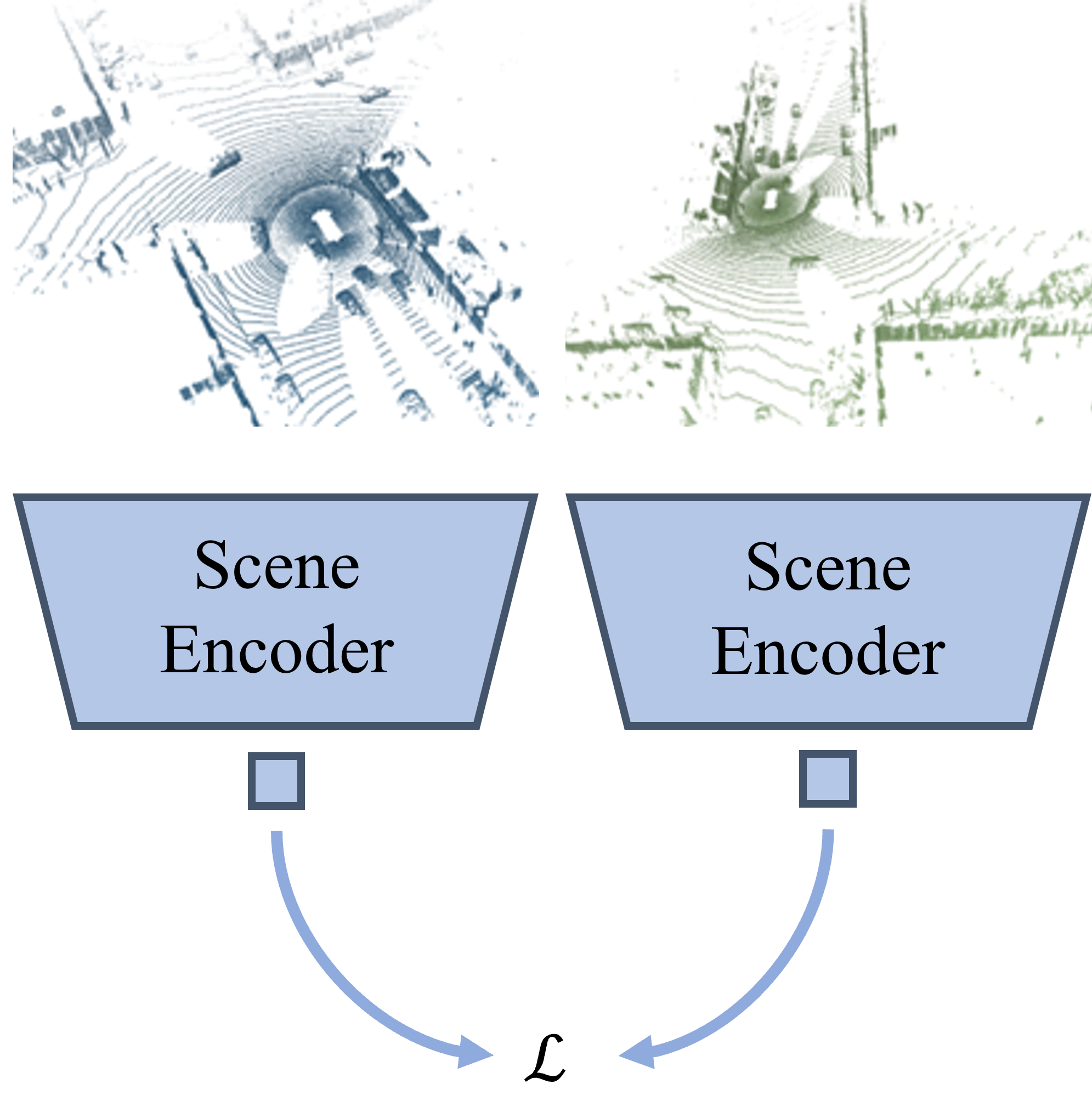
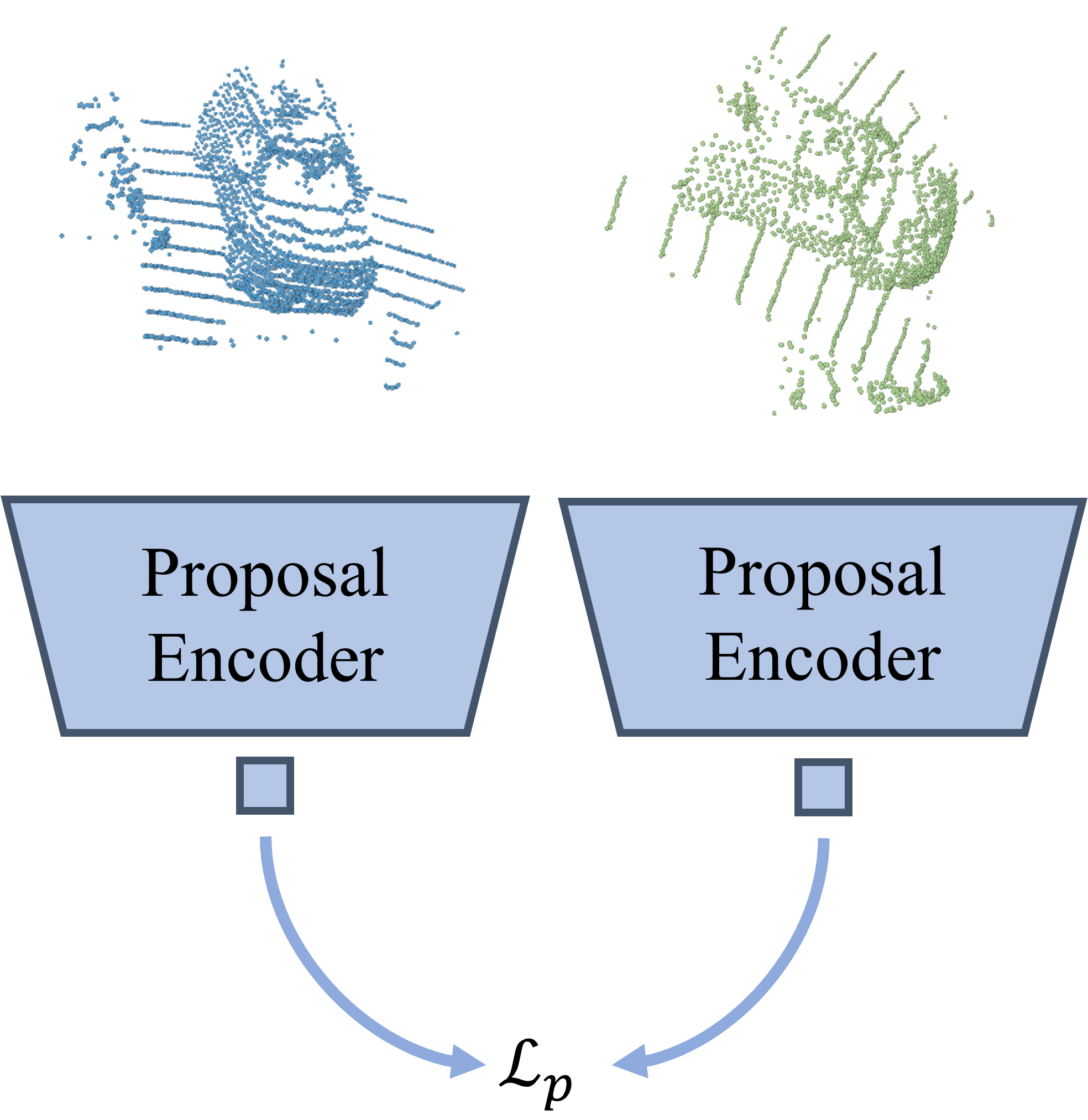
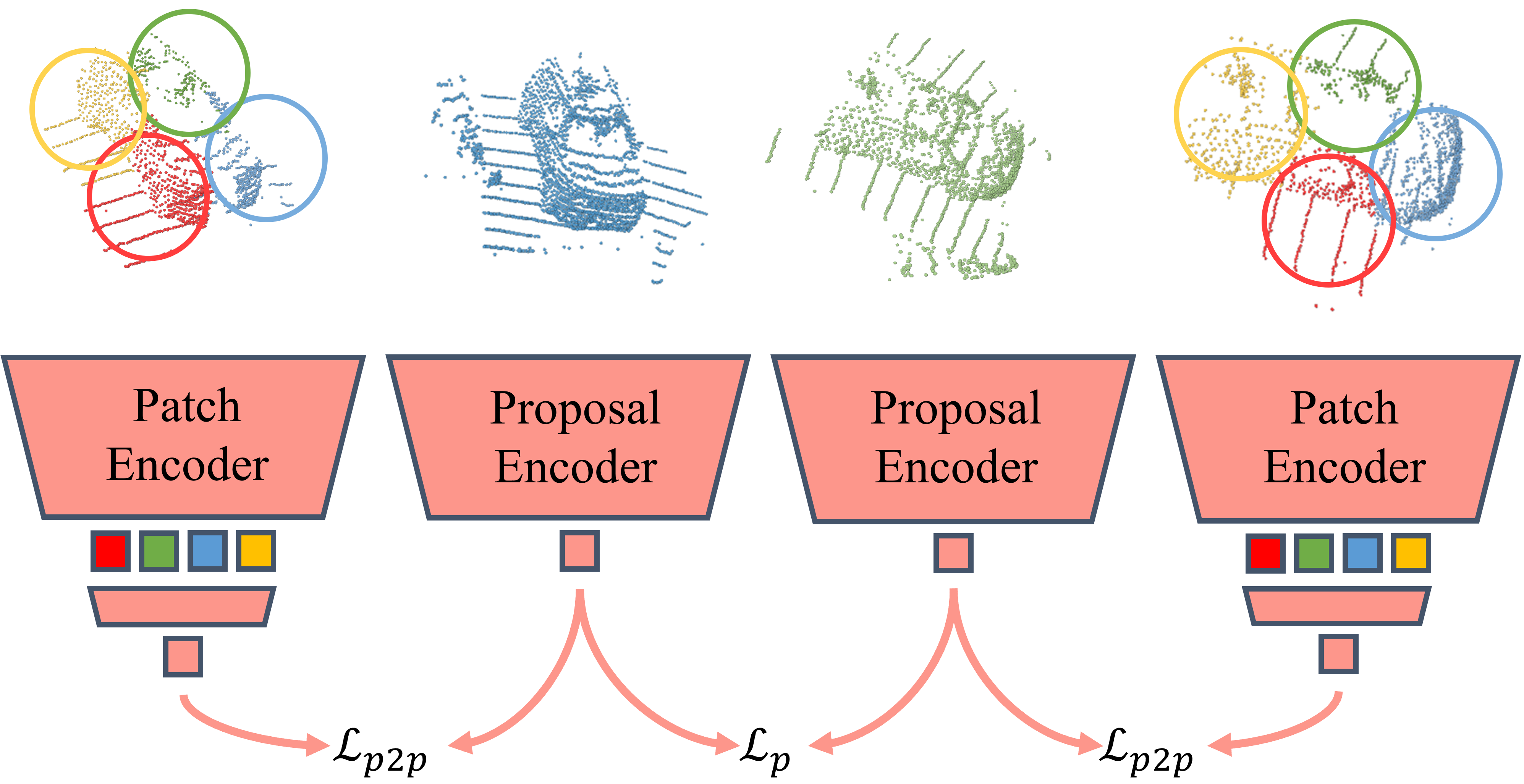
(a) DepthContrast [7]	(b) ProposalContrast [10]	(c) PatchContrast (Ours)

Figure 1: PatchContrast overview. Contrastive learning frameworks for object detection focus on different levels of abstraction. (a) DepthContrast [7] learns by contrasting a scene-level (global) representation. (b) ProposalContrast [10] learns by contrasting a proposal-level (object) representation. (c) Our PatchContrast learns by contrasting two levels: proposals and patches which inform localization and classification respectively.

2 Related Work

Hereafter, we present an overview of existing research in three relevant fields.

Supervised 3D object detecion. Object Detection refers to the task of localizing and classifying objects in a given scene. 3D methods can be divided into three categories: point-based [4, 13, 14, 15], grid-based [1, 16, 17, 18, 19, 20, 21, 22, 23, 24, 25, 26, 27], and hybrid point-voxel approaches [2, 3, 28]. Point-based methods extract features directly from the raw point cloud usually using PointNet-like architectures [29, 30], while grid-based methods transform the point cloud into a regular representation, i.e. voxels or a 2D Bird-Eye View (BEV), and utilize 3D or 2D convolutional networks. These three approaches are supervised, necessitating ground truth labels for each object in the scene during learning. To circumvent the laborious task of labeling 3D data, self-supervised approaches offer an alternative. They enable pre-training of models on large, unlabeled datasets and subsequent fine-tuning on smaller labeled datasets.

Self-supervised learning in 2D. Self-supervised learning (SSL) refers to methods that process unlabeled data to derive valuable representations for downstream learning tasks. These techniques can be categorized as generative approaches [31, 32, 33] or discriminative methods [34, 35, 36, 37, 38, 39, 40]. For a comprehensive review, please refer to [41]. Among discriminative methods, contrastive learning pre-training methods have demonstrated competitive performance compared to supervised pre-training [35, 37, 38]. However, the complexity of the data presents distinct challenges for 3D detection, as described next.

Self-supervised learning in 3D. The application of contrastive learning in the context of 3D processing has received less attention compared to its use in 2D processing. Previous studies have mainly focused on developing a representations for individual objects, which can be employed in tasks such as classification [9, 42, 43, 44, 45, 46, 47, 48, 49], reconstruction [42, 46, 50], and part segmentation [42, 43, 45, 46, 47, 48]. Recent works have introduced techniques for 3D object detection [6, 7, 8, 51]. DepthContrast [7] proposes a cross-modal contrastive learning method that leverages information from both 3D point clouds and voxel representations. PointContrast [6] utilizes contrastive learning on sampled points between two views of a point cloud scene. GCC-3D [8] presents a two-step pre-training framework, where a 3D encoder is initially trained using a geometric-aware contrast module, and then the 3D and 2D encoders are further trained with harmonized pseudo-instance clustering. ALSO [51] estimates the surface of a scene using an implicit representation (occupancy) and self-supervises through a reconstruction loss. These approaches demonstrate performance improvements compared to supervised training with limited data. However, they have not fully capitalized on the fact that the core region of interest should be at the object-level, rendering local or global representations insufficiently discriminative. A recent work, ProposalContrast [10], proposes learning an object-level representation by contrasting local subsets (proposals). Building on this approach for localization, we show how contrasting proposals also with their constituent patches further improves detection. Intuitively, this is so since the inter-relations between the components of an object are very informative. We propose a cross-level loss that encodes proposal-level information into the patch-level and vice versa.

3 PatchContrast framework

We present a novel approach for self-supervised pre-training in 3D object detection, called PatchContrast. It offers a promising alternative to fully-supervised methods when annotated data is scarce. It is built upon two main ideas: (1) extracting semantic features at the proposal level to aid in localization, and (2) extracting local features at the patch level to enable region discrimination, which is essential for classification. Our framework is general and can pre-train any 3D backbone used in 3D detectors; the weights of the pre-trained backbone can then be used in the downstream detection task. In Section 4 we present results for two widely-used backbones employed in current detectors [1, 2, 3, 17, 20]. The PatchContrast framework has three components, shown in Fig. 2: Proposal feature extraction, Patch feature extraction, and Region discrimination. We elaborate on each component below.

3.1 Proposal feature extraction

This module aims to extract small subsets, proposals, from the scene where objects are likely to appear and learn a semantically discriminative representation for each of them. The module takes as input three scene views: the input cloud $S_{0}$, as well as $S_{1},S_{2}$, obtained by applying two transformations, $T_{1},T_{2}$ on $S_{0}$. The transformations are sampled randomly from a family of augmentations, such as rotation, scaling, and dropout (see the supplemental for the family of augmentations). We note that the views $S_{i}\in\mathbb{R}^{N_{i}\times d}$, where $N_{i}$ is the number of points in $S_{i}$ and $d$ is the number of input channels for each point (e.g., $x,y,z$ and intensity). These different views are crucial for our contrastive learning process.

Two parallel branches are utilized: one to generate proposals and the second for extracting features from the scene for each proposal. In the first branch (middle in Fig. 2(a)), we aim to capture object-level geometric information for the two augmented views $S_{1},S_{2}$, by leveraging proposals. The proposals should capture subsets of the scene that are likely to contain objects and cover the regions of interest in the scene. All the proposals from both views will later be used for finding positive and negative examples in the proposal-level contrastive loss (see Section 3.3).

Specifically, the proposal extractor proceeds as follows. It first employs the RANSAC algorithm [52] to fit a plane to the input scene $S_{0}$ and remove points on the background (i.e., road). Next, it identifies the subset of non-background points in $S_{0}$ that are present in both views $S_{1}$ and $S_{2}$. This subset provides a correspondence mapping between $S_{1}$ and $S_{2}$ that will be used for contrastive learning. From this subset, $N$ query points are sampled, using Furthest Point Sampling (FPS) to encourage scene coverage. Finally, proposal $S_{pr}^{i}$ is defined as a subset of points from $S_{i}$ that fall within a fixed-radius sphere centered around a query point.

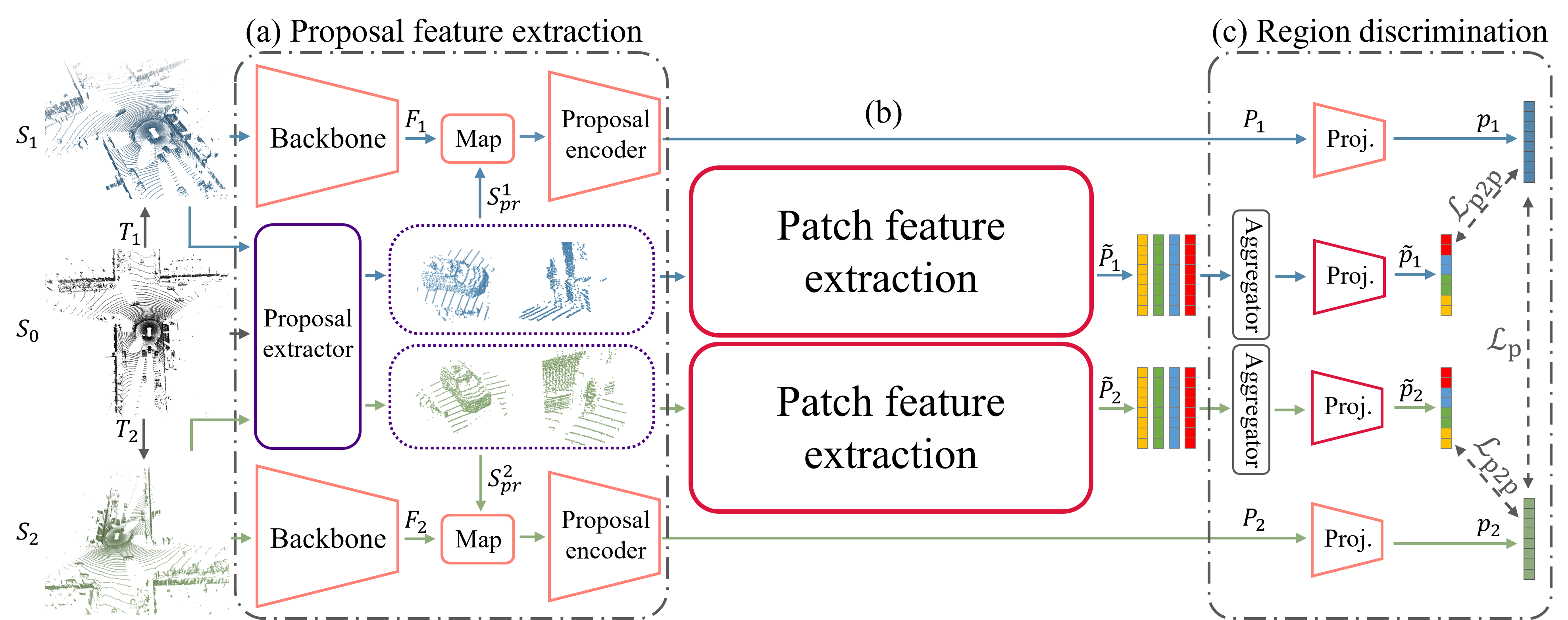
Figure 2: PatchContrast framework. (a) Given a point cloud $S_{0}$ with two augmented views $S_{1},S_{2}$, we first extract proposals from each view. Scene view features $F_{1},F_{2}$ are then extracted using a backbone and mapped onto the proposals $S^{1}_{pr},S^{2}_{pr}$. To get proposal-level features $P_{1},P_{2}$ we feed them into a proposal encoder. (b) Simultaneously, we feed the proposals into the patch feature extraction module, where patches are extracted and encoded from each proposal to get patch-level features $\tilde{P}_{1},\tilde{P}_{2}$ (see Fig. 3). (c) Finally, the region discrimination module enforces similarity between matching proposals from the two views and between a proposal and its composing patches.

Recall that our objective is to pre-train a 3D backbone, which encodes the scene into a spatial-aware representation vector. Thus, the primary aim of the second branch (upper and lower in Fig. 2(a)) is to extract a local embedding for each proposal, given its respective scene view representation vector. As current 3D detectors typically operate on a projected 2D Bird-Eye View (BEV) [1, 2, 3, 17, 20], our backbone consists of a 3D detector backbone and a 2D encoder. The weights of the 3D backbone will be transferred to the downstream detection task. The 3D backbone extracts features from each scene view, which are then projected onto the BEV space and encoded by the 2D encoder. The result is a feature map on a 2D grid, $F_{i}$, with dimension $H\times W\times C$, where $H\times W$ represents the 2D spatial subdivision of XY plane, and $C$ represents the feature dimension.

Finally, to learn a semantic representation for each proposal using the backbone-encoded feature vector $F_{i}$ and the extracted proposals from the corresponding scene view $S_{i}$, we adopt an approach similar to anchor-based detectors [2, 3, 17, 20]. First, we project each proposal $S_{pr}^{i}$ onto the BEV space to identify relevant features in $F_{i}$ for each point in the proposal. Since $F_{i}$ is a grid feature map, features are assigned to each point using bilinear interpolation. This is done for all points in all proposals, resulting in a set of per-point proposal features. To obtain a semantic representation for the entire proposal, we use a point-based encoder to encode and aggregate over all the points within the proposal, generating the proposal embedding set $P_{i}\in\mathbb{R}^{N\times C}$.

3.2 Patch feature extraction module

Given a proposal, we divide it into patches. Each patch is expected to capture valuable local information about the individual parts of the proposals, which could aid in the classification of objects. The two-stage process of our patch feature extraction module includes patch encoding and patch refinement, as shown in Fig. 3.

Patch encoding. This stage, illustrated in Fig. 3(a), aims to extract patches from each proposal and encode them into meaningful local representation vectors. A patch is a subset of points of a given proposal, where the union of the patches should cover the proposal.

Our patch extractor operates in the following manner: Initially, four keypoints are selected through the following process: Given a spherical proposal $S_{pr}^{i}$ with center coordinates $q_{0}=(x_{0},y_{0},z_{0})$, we define the candidate initial centers as $(x_{0}\pm t,y_{0},z_{0}),(x_{0},y_{0}\pm t,z_{0})$, where $t$ represents a translation. Each patch’s new origin is set to be the closest point to the candidate center. It should be noted that due to the fact that the initial proposal’s center altitude coordinate $z_{0}$ is sampled from non-background points, the keypoints (and consequently, the patches) are likely to belong to an object.

To create a patch representation, we start by encoding the scene view features $F_{i}$ into each patch. This is accomplished by mapping the features from $F_{i}$ onto each of the patch’s points, feeding them through a point-based encoder, and aggregating them to generate a per-patch feature vector $\tilde{P}_{i}\in\mathbb{R}^{N\times m\times C}$. Here $m$ is the number of patches. Since the proposals are intended to capture objects, the resulting patches are highly likely to represent object components, thereby encoding valuable semantic information about them.

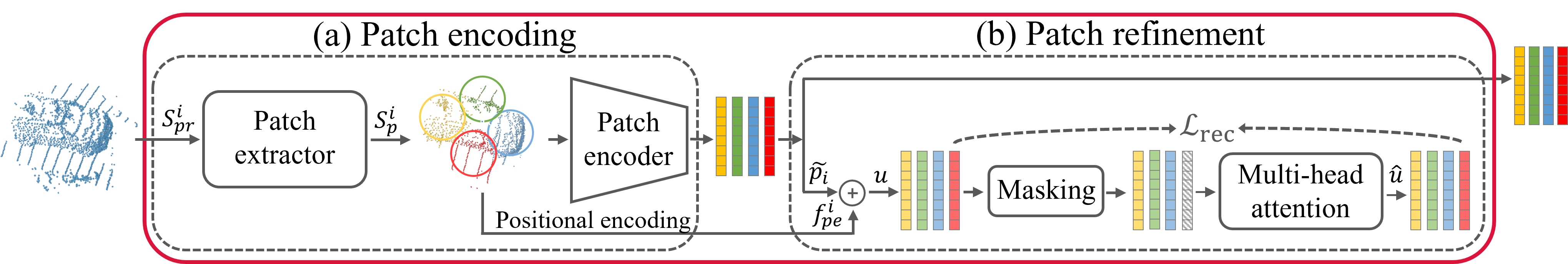
Figure 3: Patch feature extraction module. (a) Given a proposal, we extract and encode patches for patch-level representation. (b) Then, we refine the patches’ representations using a masked attention auxiliary task. This is done by masking one patch embedding and reconstructing it by leveraging information from its neighbors’ embeddings.

Patch refinement. The goal of this sub-module is to enhance the informativeness of the patch embedding (Fig. 3(b)). To achieve this objective, we suggest using an auxiliary task that modifies the representation of a patch by leveraging its neighboring patches. Intuitively, suppose that we mask one of the patches of a vehicle, for example, the one containing a tire. As humans, it is a straightforward task to determine what lies behind the mask, since the global context provides enough information to deduce spatial relationships [53]. Our patch refinement approach is inspired by this human ability.

We propose an approach to enhance the representation of patches by incorporating spatial relationship information into their high-dimensional embeddings. This is achieved through the combination of masked attention and positional encoding techniques. The masked attention mechanism takes all four patch embeddings as input, masks one of them, and reconstructs it using the remaining three. However, when dealing with proposals containing patches from different objects, the traditional masked attention approach may not yield informative results and could introduce noise. For instance, when a proposal consists of patches from both the Vehicle and the Pedestrian categories, masking out a patch embeddings from the Vehicle and using a Pedestrian patch for the reconstruction might not produce informative results. To address this issue, we add positional encoding, which encodes the normalized center coordinates of patches. This encoding provides spatial information about the patches’ relationships, allowing the masked attention mechanism to give more weight to the correlated patches and produce more accurate representations.

Formally, let $q_{p}=(x_{p},y_{p},z_{p})$ denote the center of a patch $S_{p}^{i}$ within a proposal $S_{pr}^{i}$ that is centered at $q_{pr}=(x_{pr},y_{pr},z_{pr})$ and let $\tilde{p}_{i}\in\tilde{P}_{i}$ be the associated encoded feature of $S_{p}^{i}$. We obtain the normalized center of $S_{p}^{i}$ as $\bar{q}_{p}=(x_{p}-x_{pr},y_{p}-y_{pr},z_{p}-z_{pr})$. To add the relative positional encoding feature $f^{i}_{pe}(\bar{q}_{p})\in\mathbb{R}^{C}$ that accounts for the spatial relationship between the patches, we project $\bar{q}_{p}$ using a single hidden layer MLP. As a result, the input to the masked attention is given by $u=f^{i}_{pe}(\bar{q}_{p})+\tilde{p}_{i}$.

The masked attention is trained using cosine similarity as the loss function. Specifically, the loss encourages similarity between the original patch embedding $u$ and its reconstructed embedding $\hat{u}$ from the masked attention. The loss is defined as:

$$\mathcal{L}_{rec}=1-\frac{u^{T}\hat{u}}{\|u\|\|\hat{u}\|}.$$ (1)

3.3 Region discrimination

The objective of this module is to learn a discriminative representation of a region, consisting of a proposal and its associated patches. Specifically, we are given matched proposals representation vectors from the two scene views, along with their associated patches representation vectors. We propose to employ two contrastive learning losses. The first loss is between matching proposals, promoting similarity between the two views at the proposal level. The second loss focuses on the relationship between a proposal in a certain view and its constituent patches, refining the representation of the proposal.

For the proposal loss, let $P_{1},P_{2}\in\mathbb{R}^{N\times C}$ be $N$ proposal representation sets from the scene views $S_{1},S_{2}$ respectively. We project $P_{1},P_{2}$ using a proposal projector (one hidden layer MLP) and merge the output projections to form $P$. Here, $P$ is a set with $2N$ samples, such that $p_{2k}\in P$ matches $p_{2k-1}\in P$ and $k\in[1,N]$ i.e., two consecutive elements in $P$ are positive samples. The rest $2(N-1)$ samples are negatives of $p_{2k}$ and $p_{2k-1}$. The loss between matching proposals is defined as

$$\mathcal{L}_{p}=\frac{1}{2N}\sum_{k=1}^{N}\bigl{(}\ell(p_{2k},p_{2k-1})+\ell(p_{2k-1},p_{2k})\bigr{)}.$$ (2)

In Equation 2 $\ell(p_{i},p_{j})$ is the NT-Xent loss [37], which is defined as

$$\ell(p_{i},p_{j})=-\log\frac{\exp{(\text{sim}(p_{i},p_{j})/\tau)}}{\sum_{k=1}^{2N}\mathbbm{1}_{[k\neq i]}\exp{(\text{sim}(p_{i},p_{k})/\tau)}},$$ (3)

for a positive pair $(p_{i},p_{j})$. In this equation, $\text{sim}(p_{i},p_{j})=p_{i}^{T}p_{j}/\|p_{i}\|\|p_{j}\|$ is the cosine similarity between $p_{i}$ and $p_{j}$, and $\tau$ denotes the temperature parameter.

For the patch loss, let $\tilde{P}_{1},\tilde{P}_{2}\in\mathbb{R}^{N\times m\times C}$ be patch representations with $m$ patches in each of the $N$ proposals. We first aggregate all the patch representations within each proposal, to form a single patch-level representation. This aggregated representation can be used as a positive or negative sample against the proposals. Next, we employ a patch projector, which is a one-hidden-layer MLP, to project the aggregated output. The output projections are then merged to obtain the final representation $\tilde{P}$. Here, $\tilde{P}$ is a set comprising $2N$ samples, where each $\tilde{p}_{k}\in\tilde{P}$ corresponds to the matching sample for $p_{k}\in P$ for $k\in[1,2N]$. Therefore, the second loss, which measures the dissimilarity between a proposal representation and its corresponding patch-level representation, is defined as

$$\mathcal{L}_{p2p}=\frac{1}{4N}\sum_{k=1}^{2N}\bigl{(}\ell(p_{k},\tilde{p}_{k})+\ell(\tilde{p}_{k},p_{k})\bigr{)}.$$ (4)

The overall loss is computed as a weighted sum of the two losses mentioned above, along with the reconstruction loss defined in Equation 1:

$$\mathcal{L}=\lambda_{1}\mathcal{L}_{p}+\lambda_{2}\mathcal{L}_{p2p}+\lambda_{3}\mathcal{L}_{rec}.$$ (5)

4 Experiments

A major advantage of self-supervised pre-training is the ability to transfer knowledge gained from large unlabeled datasets to small annotated ones. In order to evaluate our method we conducted experiments on the most widely-used benchmarks for 3D object detection in autonomous driving, which include KITTI [12], Waymo [11], and ONCE [5]. For all the experiments we adopt Waymo for the self-supervised pre-training, where we evaluate our pre-trained backbone generalizability by transfer learning to KITTI and ONCE. We also report results within the domain, i.e., on Waymo. Specifically, we finetune several detectors [1, 2, 3, 20] on different 3D object detection benchmarks and show that our approach outperforms previous SoTA self-supervised approaches. Implementation details, ablation study, and more results are provided in the supplemental.

Datasets and metrics. Waymo [11] contains $798$ training sequences and $202$ validation sequences, resulting in $158,081$ and $40,077$ LiDAR samples, respectively. Average Precision (AP) and Average Precision weighted by Heading (APH) are used for evaluation. We report results on the two difficulty levels and $3$ classes, with the IoU threshold set as $0.7$ for Vehicle detection and $0.5$ for Pedestrian and Cyclist. KITTI’s [12] training set contains $7,481$ examples that are divided into a training subset, with $3,712$ examples, and a validation subset, with $3,769$ examples [54]. A mean Average Precision (mAP) with $40$ recall positions is used for evaluation [55]. For precision and recall we use the standard IoU thresholds of $0.7$ for the Car class and $0.5$ for Pedestrian, and Cyclist classes. ONCE [5] contains $1M$ scenes, most of which are unannotated. For supervised training/finetuning, there are $4,961$ and $3,321$ annotated scenes in the train and validation splits, respectively. For unsupervised pre-training, the dataset contains 3 subsets, with different amounts of unlabeled data: $U_{s}$, $U_{m}$, and $U_{l}$, corresponding to $100K$, $500K$ and $1M$ scenes, respectively. An orientation-aware AP, which accounts for object orientations, is used for evaluation.

4.1 Transfer learning for 3D detection

Table 1: Transfer learning on KITTI. Our approach outperforms previous SoTA methods, especially when a limited number of labels are available. Green signifies an increase in comparison to Scratch.

Labels	Method	mAP	Car			Pedestrian			Cyclist
		Mod.	Easy	Mod.	Hard	Easy	Mod.	Hard	Easy	Mod.	Hard
20%	Scratch	66.71	91.81	82.52	80.11	58.78	53.33	47.61	86.74	64.28	59.53
	ProposalContrast [10]	68.13(+1.42)	91.96	82.65	80.15	62.58	55.05	50.06	88.58	66.68	62.32
	PatchContrast (Ours)	70.75(+4.04)	91.81	82.63	81.83	65.95	57.77	52.94	90.54	71.84	67.25
50%	Scratch	69.63	91.77	82.68	81.9	63.70	57.10	52.77	89.77	69.12	64.61
	ProposalContrast [10]	71.76(+2.13)	92.29	82.92	82.09	65.82	59.92	55.06	91.87	72.45	67.53
	PatchContrast (Ours)	72.39(+2.76)	91.78	84.47	82.23	68.21	60.76	54.84	90.59	71.94	67.37
100%	Scratch	70.57	-	84.50	-	-	57.06	-	-	70.14	-
	GCC-3D [8]	71.26(+0.69)	-	-	-	-	-	-	-	-	-
	STRL [9]	71.46(+0.89)	-	84.70	-	-	57.80	-	-	71.88	-
	PointContrast[6]	71.55(+0.98)	91.40	84.18	82.25	65.73	57.74	52.46	91.47	72.72	67.95
	ProposalContrast [10]	72.92(+2.35)	92.45	84.72	82.47	68.43	60.36	55.01	92.77	73.69	69.51
	ALSO [51]	72.96(+2.39)	-	84.68	-	-	60.16	-	-	74.04	-
	PatchContrast (Ours)	72.97(+2.40)	92.08	84.67	82.35	66.95	59.92	54.43	91.83	74.33	69.83

Transfer learning on KITTI dataset. We finetune with different amounts of labeled data of the train split and report on the entire validation split, as in [7, 10]. Specifically, we split the train set to $20\%$, $50\%$, and $100\%$, resulting in $\sim 0.7K$, $\sim 1.9K$ and $3.7K$ scenes, respectively. Table 1 reports the results on the KITTI 3D detection benchmark for PV-RCNN [2] detector. The results show that for all splits our approach improves the performance over training from scratch. An important observation is that the improvement is higher whenever less labeled data is available. When all training examples are available ($100\%$) we achieve on-par results with [10, 51]. However, with a limited number of annotated samples, we achieve better results than training from scratch on the full annotated dataset. Specifically, on the Moderate level, we improve the baseline (with $100\%$ annotations) by $0.18$ and $1.82$ when trained with only $20\%$ and $50\%$ annotations, respectively.

Object detection on Waymo dataset. In order to assess the quality of our pre-trained backbone’s embedding for detection, we evaluate on Waymo. We follow the common protocol of [56] and finetune with $20\%$ labeled examples ($\sim 31.6K$ scenes) from the train set for $30$ epochs and evaluate on the validation set. Table 2 reports the results on Level-2 to other SoTA pre-training methods: GCC-3D [8], ProposalContrast [10], and DepthContrast [7]. To show that our approach is general, we report on three different detectors  [1, 2, 3] with two variants of the backbone architecture: VResBB, and VBB (see supplementary for backbone details). The results show that our approach achieves improved performance over the baseline (training from scratch), as well as outperforming other methods. See supplemental for results on Level-1. Note that our approach improves the results, even though it strictly uses only the training split data for pre-training (some methods also use the validation split).

Table 2: 3D object detection on Waymo. We pre-train two backbones (VResBB, and VBB) and finetuned three detectors on $20\%$ of Waymo train set. ${\dagger}$ indicates our reproduction using their code (as the papers do not report on the respective detector).

Method	Avg. (L2)		Vehicle (L2)		Ped. (L2)		Cyc. (L2)
	AP	APH	AP	APH	AP	APH	AP	APH
PV-RCNN [8] (VResBB)	59.84	56.23	64.99	64.38	53.80	45.14	60.72	59.18
+ GCC-3D [8]	61.30(+1.83)	58.18(+1.95)	65.65	65.10	55.54	48.02	62.72	61.43
+ ProposalContrast [10]	62.62(+2.78)	59.28(+3.05)	66.04	65.47	57.58	49.51	64.23	62.86
+ PatchContrast (Ours)	66.51(+6.67)	62.87 (+6.64)	67.23	66.65	65.32	56.42	66.98	65.56
PV-RCNN [2] (VBB)	64.84	60.86	67.44	66.80	63.70	53.95	63.39	61.82
+ DepthCont. [7] †	65.04(+0.20)	60.96(+0.10)	67.15	66.52	63.82	53.97	64.15	62.38
+ PatchContrast (Ours)	65.51(+0.67)	61.45(+0.59)	67.12	66.48	64.03	54.16	65.37	63.70
PV-RCNN++ [3] (VBB)	69.43	66.87	69.07	68.62	69.92	63.74	69.31	68.26
+ DepthCont [7] †	69.46(+0.03)	66.95(+0.08)	68.99	68.53	70.59	64.59	68.79	67.73
+ PatchContrast (Ours)	69.56(+0.13)	67.02(+0.15)	69.17	68.72	70.95	64.89	68.54	67.45
CenterPoint [1] (VResBB)	63.46	60.95	61.81	61.30	63.62	57.79	64.96	63.77
+ GCC-3D [8]	65.29(+1.83)	62.79(+1.84)	63.97	63.47	64.23	58.47	67.68	66.44
+ ProposalContrast [10]	66.42(+2.96)	63.85(+2.90)	64.94	64.42	66.13	60.11	68.19	67.01
+ PatchContrast (Ours)	66.82(+3.36)	64.38(+3.43)	64.81	64.32	67.16	61.49	68.51	67.32

Table 3: Label efficiency on Waymo. We train with the standard protocol with different amounts of labeled data and report results on Waymo Level-2. Our approach benefits from fewer labeled data.

Labels	Method	Average		Vehicle		Pedestrian		Cyclist
		AP	APH	AP	APH	AP	APH	AP	APH
1% ($\sim 1.6K$ frames)	CenterPoint [1]	50.10	47.25	49.51	48.86	48.59	41.98	52.20	50.92
	PatchContrast (Ours)	52.23(+2.13)	49.33(+2.08)	51.08	50.41	51.01	44.42	54.60	53.16
5% ($\sim 7.9K$ frames)	CenterPoint [1]	61.47	58.84	59.42	58.90	61.25	55.22	63.73	62.40
	PatchContrast (Ours)	62.04(+0.57)	59.40(+0.56)	60.20	59.69	61.21	55.17	64.69	63.32
10% ($\sim 15.8K$ frames)	CenterPoint [1]	63.91	61.39	62.40	61.90	63.72	57.90	65.60	64.38
	PatchContrast (Ours)	64.56(+0.65)	62.06(+0.67)	62.57	62.07	64.21	58.44	66.89	65.66

Table 4: Transfer learning on ONCE. Our framework outperforms previous approaches, even when pre-trained on a different dataset.

Method	Pre-trained dataset	mAP	Vehicle	Pedestrian	Cyclist
SECOND [20]	-	51.89	71.19	26.44	58.04
+ BYOL [39]	$U_{s}$	46.04(-5.85)	68.02	19.50	50.61
+ PointContrast [6]	$U_{s}$	49.98(-1.91)	71.07	22.52	56.36
+ SwAV [38]	$U_{s}$	51.96(+0.07)	72.71	25.13	58.05
+ DeepCluster [57]	$U_{s}$	52.06(+0.17)	73.19	24.00	58.99
+ ALSO [51]	$U_{s}$	52.68(+0.79)	71.73	28.16	58.13
+ DepthContrast [7] †	Waymo	52.21(+0.32)	71.93	26.77	57.93
+ PatchContrast (Ours)	Waymo	54.18(+2.29)	73.35	30.87	58.33

Label efficiency on Waymo dataset. In this experiment, we evaluate the performance of our pre-trained backbones under a label-efficient setting i.e., with different amounts of labeled data. Specifically, we finetune CenterPoints [1] with $1\%$, $5\%$, and $10\%$ of Waymo’s [11] train set for $30$ epochs, and evaluate on the validation set. The results, reported in Table 4, clearly show that our pre-trained framework provides significant benefits when fewer labeled samples are available, thus providing a good alternative to supervised approaches when labeled data is limited.

Transfer learning on ONCE dataset. We further evaluate our backbones’ generalizability on ONCE [5] dataset. We pre-train on Waymo, as in the previous experiments, finetune SECOND [20] on ONCE’s train set and evaluate on the validation set. Table 4 report on the official self-supervised benchmark results and compares to other SoTA approaches. It clearly shows that even when pre-trained on a different dataset, our method improves the baselines and outperforms previous methods.

4.2 Insights

To gain insights into our results, we performed clustering on the scene’s points in the embedding space using the k-means algorithm. Each point was assigned a cluster ID, and the points were colored accordingly. Fig. 4 illustrates a typical outcome, obtained from our pre-trained VBB backbone. The results demonstrate that the embedding space of the backbone captures a semantic representation of objects. For instance, cars are clustered together (grey, golden, and pink). Moreover, our approach successfully captures local information about objects and their constituent parts. As an example, the front right wheels of all cars are grouped in the same cluster, indicated by the color pink. This ability to capture the structural information can be attributed to our patch-level abstraction learning. Furthermore, since our approach is self-supervised and does not rely on labeled data, it can locate objects that do not fall into pre-defined classes. For instance, it detects the traffic sign within the green rectangle on the right, even though it is not part of the pre-defined categories.

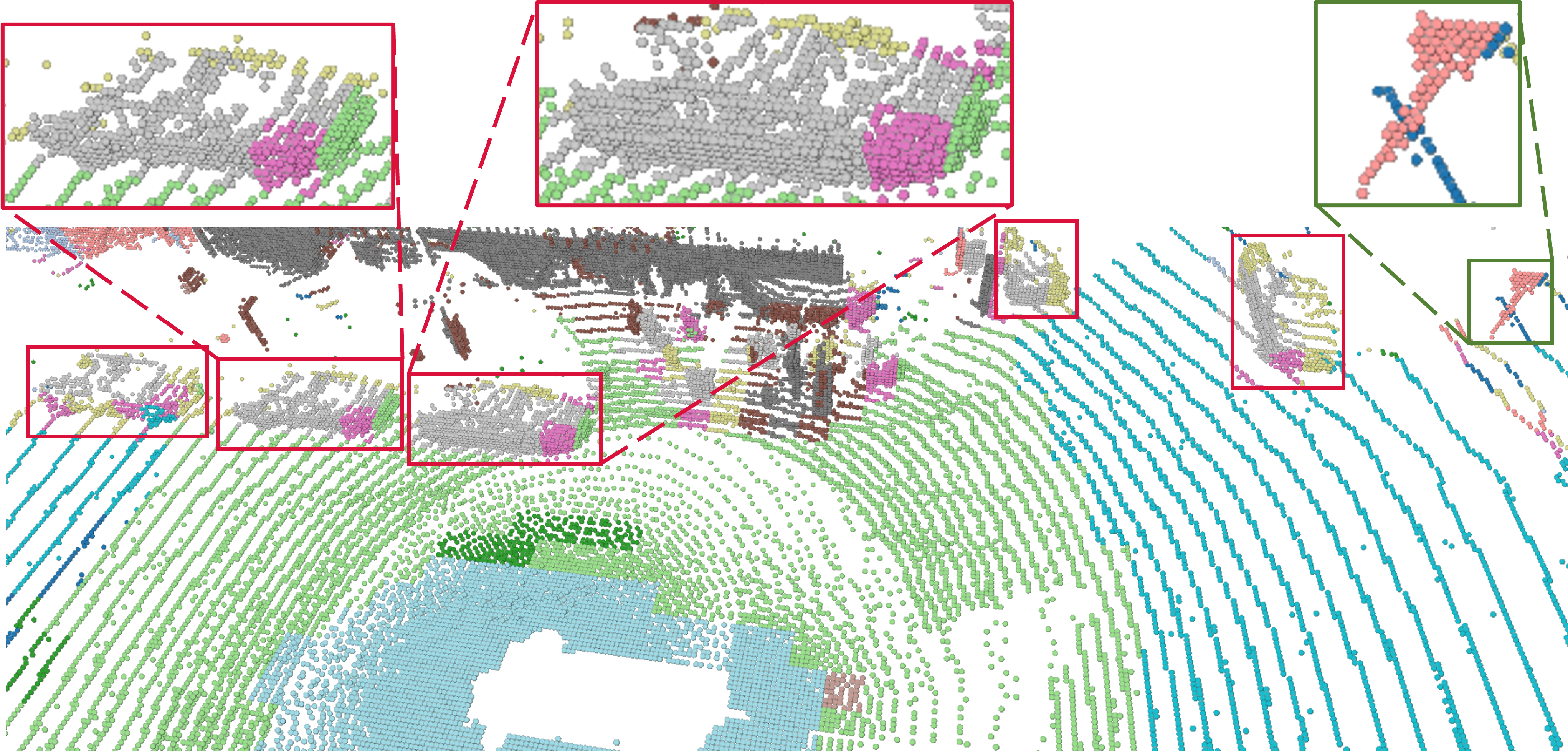
Figure 4: Qualitative result. When clustering the embeddings, we can observe semantically meaningful object components, such as cars (grey) and wheels (pink). Remarkably, these meaningful components are discovered without any supervision.

Limitations. In comparison to the approach of extracting only proposals that cover the regions of interest [10], our method additionally extracts patches. Our improved performance comes at the cost of an increased number of parameters in the overall framework, leading to higher memory consumption and longer training time. A larger number of parameters are also required for fine-tuning.

Broader impact. Self-supervised 3D detection algorithms improve object detection without heavy reliance on labeled data. This approach enhances scalability, versatility, and reduces dependency on human annotation. However, the reliance on unlabeled data might increase computational complexity and raise ethical concerns regarding privacy and data security. Addressing these issues is essential for the practical implementation of autonomous driving.

5 Conclusion

We introduced a self-supervised pre-training framework, called PatchContrast, for 3D object detection. PatchContrast incorporates two levels of abstraction: proposal level and patch level, enabling the learning of discriminative embedding. Patches reveal the inter-relation between the components of the object within the proposal. These inter-relations, refined through an auxiliary task, allow for contrasting different representations of the proposal, considering both its components and the proposal as a whole. Through the combination of the levels of abstraction, PatchContrast effectively learns discriminative representations for the detection task. We validated the efficacy of PatchContrast on three widely-used 3D object detection datasets, surpassing previous state-of-the-art approaches. Additionally, our results demonstrated that pre-training on large unlabeled data can significantly enhance detection accuracy, particularly when labeled data is limited.

References

- [1] T. Yin, X. Zhou, and P. Krahenbuhl, “Center-based 3d object detection and tracking,” in Proceedings of the IEEE/CVF conference on computer vision and pattern recognition, 2021, pp. 11 784–11 793.
- [2] S. Shi, C. Guo, L. Jiang, Z. Wang, J. Shi, X. Wang, and H. Li, “Pv-rcnn: Point-voxel feature set abstraction for 3d object detection,” in Proceedings of the IEEE/CVF Conference on Computer Vision and Pattern Recognition, 2020, pp. 10 529–10 538.
- [3] S. Shi, L. Jiang, J. Deng, Z. Wang, C. Guo, J. Shi, X. Wang, and H. Li, “Pv-rcnn++: Point-voxel feature set abstraction with local vector representation for 3d object detection,” International Journal of Computer Vision, vol. 131, no. 2, pp. 531–551, 2023.
- [4] S. Shi, X. Wang, and H. Li, “Pointrcnn: 3d object proposal generation and detection from point cloud,” in Proceedings of the IEEE/CVF conference on computer vision and pattern recognition, 2019, pp. 770–779.
- [5] J. Mao, M. Niu, C. Jiang, H. Liang, J. Chen, X. Liang, Y. Li, C. Ye, W. Zhang, Z. Li et al., “One million scenes for autonomous driving: Once dataset,” arXiv preprint arXiv:2106.11037, 2021.
- [6] S. Xie, J. Gu, D. Guo, C. R. Qi, L. Guibas, and O. Litany, “Pointcontrast: Unsupervised pre-training for 3d point cloud understanding,” in Computer Vision–ECCV 2020: 16th European Conference, Glasgow, UK, August 23–28, 2020, Proceedings, Part III 16. Springer, 2020, pp. 574–591.
- [7] Z. Zhang, R. Girdhar, A. Joulin, and I. Misra, “Self-supervised pretraining of 3d features on any point-cloud,” in Proceedings of the IEEE/CVF International Conference on Computer Vision, 2021, pp. 10 252–10 263.
- [8] H. Liang, C. Jiang, D. Feng, X. Chen, H. Xu, X. Liang, W. Zhang, Z. Li, and L. Van Gool, “Exploring geometry-aware contrast and clustering harmonization for self-supervised 3d object detection,” in Proceedings of the IEEE/CVF International Conference on Computer Vision, 2021, pp. 3293–3302.
- [9] S. Huang, Y. Xie, S.-C. Zhu, and Y. Zhu, “Spatio-temporal self-supervised representation learning for 3d point clouds,” in Proceedings of the IEEE/CVF International Conference on Computer Vision, 2021, pp. 6535–6545.
- [10] J. Yin, D. Zhou, L. Zhang, J. Fang, C.-Z. Xu, J. Shen, and W. Wang, “Proposalcontrast: Unsupervised pre-training for lidar-based 3d object detection,” in Computer Vision–ECCV 2022: 17th European Conference, Tel Aviv, Israel, October 23–27, 2022, Proceedings, Part XXXIX. Springer, 2022, pp. 17–33.
- [11] P. Sun, H. Kretzschmar, X. Dotiwalla, A. Chouard, V. Patnaik, P. Tsui, J. Guo, Y. Zhou, Y. Chai, B. Caine et al., “Scalability in perception for autonomous driving: Waymo open dataset,” in Proceedings of the IEEE/CVF conference on computer vision and pattern recognition, 2020, pp. 2446–2454.
- [12] A. Geiger, P. Lenz, and R. Urtasun, “Are we ready for autonomous driving? the kitti vision benchmark suite,” in 2012 IEEE conference on computer vision and pattern recognition. IEEE, 2012, pp. 3354–3361.
- [13] W. Shi and R. Rajkumar, “Point-gnn: Graph neural network for 3d object detection in a point cloud,” in Proceedings of the IEEE/CVF conference on computer vision and pattern recognition, 2020, pp. 1711–1719.
- [14] Z. Yang, Y. Sun, S. Liu, and J. Jia, “3dssd: Point-based 3d single stage object detector,” in Proceedings of the IEEE/CVF conference on computer vision and pattern recognition, 2020, pp. 11 040–11 048.
- [15] Z. Yang, Y. Sun, S. Liu, X. Shen, and J. Jia, “Std: Sparse-to-dense 3d object detector for point cloud,” in Proceedings of the IEEE/CVF International Conference on Computer Vision, 2019, pp. 1951–1960.
- [16] Y. Chen, S. Liu, X. Shen, and J. Jia, “Fast point r-cnn,” in Proceedings of the IEEE/CVF International Conference on Computer Vision, 2019, pp. 9775–9784.
- [17] J. Deng, S. Shi, P. Li, W. Zhou, Y. Zhang, and H. Li, “Voxel r-cnn: Towards high performance voxel-based 3d object detection,” arXiv preprint arXiv:2012.15712, vol. 1, no. 2, p. 4, 2020.
- [18] A. H. Lang, S. Vora, H. Caesar, L. Zhou, J. Yang, and O. Beijbom, “Pointpillars: Fast encoders for object detection from point clouds,” in Proceedings of the IEEE/CVF Conference on Computer Vision and Pattern Recognition, 2019, pp. 12 697–12 705.
- [19] S. Shi, Z. Wang, J. Shi, X. Wang, and H. Li, “From points to parts: 3d object detection from point cloud with part-aware and part-aggregation network,” IEEE transactions on pattern analysis and machine intelligence, vol. 43, no. 8, pp. 2647–2664, 2020.
- [20] Y. Yan, Y. Mao, and B. Li, “Second: Sparsely embedded convolutional detection,” Sensors, vol. 18, no. 10, p. 3337, 2018.
- [21] B. Yang, M. Liang, and R. Urtasun, “Hdnet: Exploiting hd maps for 3d object detection,” in Conference on Robot Learning. PMLR, 2018, pp. 146–155.
- [22] B. Yang, W. Luo, and R. Urtasun, “Pixor: Real-time 3d object detection from point clouds,” in Proceedings of the IEEE conference on Computer Vision and Pattern Recognition, 2018, pp. 7652–7660.
- [23] M. Ye, S. Xu, and T. Cao, “Hvnet: Hybrid voxel network for lidar based 3d object detection,” in Proceedings of the IEEE/CVF conference on computer vision and pattern recognition, 2020, pp. 1631–1640.
- [24] W. Zheng, W. Tang, S. Chen, L. Jiang, and C.-W. Fu, “Cia-ssd: Confident iou-aware single-stage object detector from point cloud,” in Proceedings of the AAAI conference on artificial intelligence, vol. 35, no. 4, 2021, pp. 3555–3562.
- [25] W. Zheng, W. Tang, L. Jiang, and C.-W. Fu, “Se-ssd: Self-ensembling single-stage object detector from point cloud,” in Proceedings of the IEEE/CVF Conference on Computer Vision and Pattern Recognition, 2021, pp. 14 494–14 503.
- [26] Y. Zhou and O. Tuzel, “Voxelnet: End-to-end learning for point cloud based 3d object detection,” in Proceedings of the IEEE conference on computer vision and pattern recognition, 2018, pp. 4490–4499.
- [27] O. Shrout, Y. Ben-Shabat, and A. Tal, “Gravos: Voxel selection for 3d point-cloud detection,” in Proceedings of the IEEE/CVF Conference on Computer Vision and Pattern Recognition, 2023, pp. 21 684–21 693.
- [28] Z. Liu, H. Tang, Y. Lin, and S. Han, “Point-voxel cnn for efficient 3d deep learning,” Advances in Neural Information Processing Systems, vol. 32, 2019.
- [29] C. R. Qi, H. Su, K. Mo, and L. J. Guibas, “Pointnet: Deep learning on point sets for 3d classification and segmentation,” in Proceedings of the IEEE conference on computer vision and pattern recognition, 2017, pp. 652–660.
- [30] C. R. Qi, L. Yi, H. Su, and L. J. Guibas, “Pointnet++: Deep hierarchical feature learning on point sets in a metric space,” Advances in neural information processing systems, vol. 30, 2017.
- [31] J. Donahue, P. Krähenbühl, and T. Darrell, “Adversarial feature learning,” arXiv preprint arXiv:1605.09782, 2016.
- [32] J. Donahue and K. Simonyan, “Large scale adversarial representation learning,” Advances in neural information processing systems, vol. 32, 2019.
- [33] L. Mescheder, S. Nowozin, and A. Geiger, “Adversarial variational bayes: Unifying variational autoencoders and generative adversarial networks,” in International conference on machine learning. PMLR, 2017, pp. 2391–2400.
- [34] A. v. d. Oord, Y. Li, and O. Vinyals, “Representation learning with contrastive predictive coding,” arXiv preprint arXiv:1807.03748, 2018.
- [35] K. He, H. Fan, Y. Wu, S. Xie, and R. Girshick, “Momentum contrast for unsupervised visual representation learning,” in Proceedings of the IEEE/CVF conference on computer vision and pattern recognition, 2020, pp. 9729–9738.
- [36] X. Chen, H. Fan, R. Girshick, and K. He, “Improved baselines with momentum contrastive learning,” arXiv preprint arXiv:2003.04297, 2020.
- [37] T. Chen, S. Kornblith, M. Norouzi, and G. Hinton, “A simple framework for contrastive learning of visual representations,” in International conference on machine learning. PMLR, 2020, pp. 1597–1607.
- [38] M. Caron, I. Misra, J. Mairal, P. Goyal, P. Bojanowski, and A. Joulin, “Unsupervised learning of visual features by contrasting cluster assignments,” Advances in neural information processing systems, vol. 33, pp. 9912–9924, 2020.
- [39] J.-B. Grill, F. Strub, F. Altché, C. Tallec, P. Richemond, E. Buchatskaya, C. Doersch, B. Avila Pires, Z. Guo, M. Gheshlaghi Azar et al., “Bootstrap your own latent-a new approach to self-supervised learning,” Advances in neural information processing systems, vol. 33, pp. 21 271–21 284, 2020.
- [40] E. Xie, J. Ding, W. Wang, X. Zhan, H. Xu, P. Sun, Z. Li, and P. Luo, “Detco: Unsupervised contrastive learning for object detection,” in Proceedings of the IEEE/CVF International Conference on Computer Vision, 2021, pp. 8392–8401.
- [41] X. Liu, F. Zhang, Z. Hou, L. Mian, Z. Wang, J. Zhang, and J. Tang, “Self-supervised learning: Generative or contrastive,” IEEE Transactions on Knowledge and Data Engineering, vol. 35, no. 1, pp. 857–876, 2021.
- [42] K. Hassani and M. Haley, “Unsupervised multi-task feature learning on point clouds,” in Proceedings of the IEEE/CVF International Conference on Computer Vision, 2019, pp. 8160–8171.
- [43] A. Alliegro, D. Boscaini, and T. Tommasi, “Joint supervised and self-supervised learning for 3d real world challenges,” in 2020 25th International Conference on Pattern Recognition (ICPR). IEEE, 2021, pp. 6718–6725.
- [44] S. Huang, Y. Xie, S.-C. Zhu, and Y. Zhu, “Spatio-temporal self-supervised representation learning for 3d point clouds,” in Proceedings of the IEEE/CVF International Conference on Computer Vision, 2021, pp. 6535–6545.
- [45] L. Zhang and Z. Zhu, “Unsupervised feature learning for point cloud by contrasting and clustering with graph convolutional neural network,” arXiv preprint arXiv:1904.12359, 2019.
- [46] J. Sauder and B. Sievers, “Self-supervised deep learning on point clouds by reconstructing space,” Advances in Neural Information Processing Systems, vol. 32, 2019.
- [47] H. Liu, M. Cai, and Y. J. Lee, “Masked discrimination for self-supervised learning on point clouds,” in Computer Vision–ECCV 2022: 17th European Conference, Tel Aviv, Israel, October 23–27, 2022, Proceedings, Part II. Springer, 2022, pp. 657–675.
- [48] Y. Pang, W. Wang, F. E. Tay, W. Liu, Y. Tian, and L. Yuan, “Masked autoencoders for point cloud self-supervised learning,” in Computer Vision–ECCV 2022: 17th European Conference, Tel Aviv, Israel, October 23–27, 2022, Proceedings, Part II. Springer, 2022, pp. 604–621.
- [49] S. Yan, Z. Yang, H. Li, L. Guan, H. Kang, G. Hua, and Q. Huang, “Implicit autoencoder for point cloud self-supervised representation learning,” arXiv preprint arXiv:2201.00785, 2022.
- [50] I. Achituve, H. Maron, and G. Chechik, “Self-supervised learning for domain adaptation on point clouds,” in Proceedings of the IEEE/CVF winter conference on applications of computer vision, 2021, pp. 123–133.
- [51] A. Boulch, C. Sautier, B. Michele, G. Puy, and R. Marlet, “Also: Automotive lidar self-supervision by occupancy estimation,” arXiv preprint arXiv:2212.05867, 2022.
- [52] M. A. Fischler and R. C. Bolles, “Random sample consensus: a paradigm for model fitting with applications to image analysis and automated cartography,” Communications of the ACM, vol. 24, no. 6, pp. 381–395, 1981.
- [53] K. He, X. Chen, S. Xie, Y. Li, P. Dollár, and R. Girshick, “Masked autoencoders are scalable vision learners,” in Proceedings of the IEEE/CVF Conference on Computer Vision and Pattern Recognition, 2022, pp. 16 000–16 009.
- [54] X. Chen, K. Kundu, Y. Zhu, A. G. Berneshawi, H. Ma, S. Fidler, and R. Urtasun, “3d object proposals for accurate object class detection,” Advances in neural information processing systems, vol. 28, 2015.
- [55] A. Simonelli, S. R. Bulo, L. Porzi, M. López-Antequera, and P. Kontschieder, “Disentangling monocular 3d object detection,” in Proceedings of the IEEE/CVF International Conference on Computer Vision, 2019, pp. 1991–1999.
- [56] O. D. Team, “Openpcdet: An open-source toolbox for 3d object detection from point clouds,” https://github.com/open-mmlab/OpenPCDet, 2020.
- [57] M. Caron, P. Bojanowski, A. Joulin, and M. Douze, “Deep clustering for unsupervised learning of visual features,” in Proceedings of the European conference on computer vision (ECCV), 2018, pp. 132–149.