Hierarchical variable clustering using singular value decomposition

Abstract

In this work, we present a novel method for hierarchically variable clustering using singular value decomposition. Our proposed approach provides a non-parametric solution to identify block diagonal patterns in covariance (correlation) matrices, thereby grouping variables according to their dissimilarity. We explain the methodology and outline the incorporation of linkage functions to assess dissimilarities between clusters. To validate the efficiency of our method, we perform both a simulation study and an analysis of real-world data. Our findings show the approach’s robustness. We conclude by discussing potential extensions and future directions for research in this field. Supplementary materials for this article can be accessed online.

1 Introduction

The study of multidimensional phenomena often requires the exploration of hierarchical structures to represent the underlying concepts. Within psychometric research, several examples of such phenomena have been described. For instance, Carroll’s three-stratum theory (Carroll, 1993) and the Cattell-Horn-Carroll theory, which combines Carroll’s three-stratum theory with Horn-Cattell’s theory (McGrew, 2009), serve to structure cognitive abilities. Likewise, personality traits, such as the Big Five, are organized into groups (Digman, 1990).

Several methodologies have been proposed to model and analyze hierarchical structures in data. In this context, Holzinger (1944) and Jöreskog (1969) derived factor models for cases where the number of factors and relations between groups are known. Cavicchia and Vichi (2022) introduced a latent factor model called second-order disjoint factor analysis, which aims to model an unknown hierarchical structure of order two. Cavicchia et al. (2022) proposed a hierarchical principal component analysis model consisting of disjoint groups of observed variables, while Vichi and Saporta (2009) presented a constrained principal component analysis for simultaneous clustering of objects and partitioning of variables.

In portfolio management and neuroscience, there are approaches that transform correlation matrices into dissimilarity matrices to cluster variables (Mantegna, 1999; Liu et al., 2012; de Prado, 2016). This way, observation-clustering methods can be applied to identify patterns and groupings. However, it is important to be cautious of misspecification issues that arise due to the greedy nature of these algorithms when applied to cluster variables (Kaufman and Rousseeuw, 1990).

There are also approaches for grouping variables based on correlation coefficients. Vigneau and Qannari (2003) discuss a non-hierarchical approach where it is desirable to cluster correlated variables, while Plasse et al. (2007) propose a clustering method specifically designed for large data with binary attributes. Soffritti (1999) provides a general comparison of measures to calculate dissimilarities of variable clusters based on the correlation coefficient.

The method proposed by Revelle (1979) suggests a hierarchical variable clustering approach based on a weighted correlation measure between a cluster and a variable outside the cluster. The number of variables can be calculated using cluster reliability.

Clustered variables are characterized by a block diagonal shape of the covariance (correlation) matrix. Previous research by Cavicchia et al. (2020) identified the clusters by reconstructing the correlation matrix through an ultrametric correlation matrix. However, apart from their work, no efforts have been made to uncover the block diagonal structure of the covariance (correlation) matrix for hierarchical variable clustering. To address this gap, we propose a non-parametric approach that directly identifies the block diagonal structure of the matrix for clustering. Our approach is based on the eigenvectors of the covariance matrix, which are obtained through singular value decomposition (SVD) of the sample. By splitting the variables divisively based on the identified structure, we can effectively cluster them. In addition to clustering, we provide methods to measure the dissimilarity between clusters. This allows us to visualize the hierarchical structure using a dendrogram.

This article is organized as follows: Section 2 introduces the necessary notation that will be used throughout the article. In Section 3, we present our novel approach to hierarchical variable clustering. We discuss the identification of clusters and provide an algorithm for conducting hierarchical variable clustering in practice. A simulation study to evaluate the performance of the model is given in Section 4. The results obtained from this study contribute to the validation of the model. In Section 5, we present a real data example that showcases the application of hierarchical variable clustering. Section 6 discusses potential extensions and future directions of the model. The code to replicate our results is included in the supplementary material.

2 Setup

We introduce some notations in this section. We consider a random vector $\bm{X}=(\bm{X}_{1},\bm{X}_{2})\in\mathbb{R}^{P+Q}$ that consists of $M=P+Q$ random variables and is divided into two subvectors $\bm{X}_{1}\in\mathbb{R}^{P}$ and $\bm{X}_{2}\in\mathbb{R}^{Q}$. We assume $\mathbb{E}(\bm{X})=\bm{0}$ such that

$$\mathbb{E}(\bm{X}\bm{X}^{\top})\equiv\bm{\Sigma}\equiv\begin{pmatrix}\bm{\Sigma}_{1}&\bm{\mathrm{E}}\\ \bm{\mathrm{E}}^{\top}&\bm{\Sigma}_{2}\end{pmatrix}\;,$$ (1)

is the covariance matrix of $\bm{X}$. The covariance matrix $\bm{\Sigma}$ consists of the covariance matrices $\bm{\Sigma}_{1}$ and $\bm{\Sigma}_{2}$ of $\bm{X}_{1}$ and $\bm{X}_{2}$ respectively, along with the covariances $\bm{\mathrm{E}}$ between these two subvectors. The eigendecomposition of the covariance matrix $\bm{\Sigma}$ is denoted as $\bm{\Sigma}=\bm{V}\bm{\Lambda}\bm{V}^{\top}$, where $\bm{\Lambda}$ is a diagonal matrix containing the non-negative eigenvalues of $\bm{\Sigma}$ in descending order, and $\bm{V}$ is an orthonormal matrix containing the respective eigenvectors. In the sample case, the right singular vectors of the sample correspond to $\bm{V}$.

For matrices, we use the Frobenius norm denoted as $\|\cdot\|_{F}$, and for vectors, we use the $\mathcal{L}_{p}$ norms denoted as $\|\cdot\|_{p}$, where $p\in\{1,\infty\}$ .

3 Hierarchical variable clustering

This section discusses hierarchical variable clustering, in which similar variables are grouped and dissimilar variables are seperated into different groups. Therefore, a measure for assessing similarity and dissimilarity between variables is required. The correlation coefficient is a natural choice for such a measure. Using the correlation coefficient, groups of variables are characterized that are strongly correlated within the group and less strongly correlated with variables outside the group. This is reflected by a block diagonal structure in the underlying covariance matrix, where the groups are represented as blocks.

We discuss the identification of the block diagonal structure to detect the variable groups. Further, we provide linkage functions to assess dissimilarity between clusters, and present an algorithm for conducting hierarchical variable clustering in practice.

3.1 Group identification

In this section, we discuss the detection of the block diagonal covariance matrix structure.

Initially, we assume no correlation between the variables contained in the subvectors $\bm{X}_{1}$ and $\bm{X}_{2}$ (i.e., $\bm{\mathrm{E}}=\bm{0}$). This simplifies the covariance matrix $\bm{\Sigma}$ given in (1) to a block diagonal matrix $\bm{\Sigma}=\mathrm{diag}(\bm{\Sigma}_{1},\bm{\Sigma}_{2})$, and we have $P$ eigenvectors of shape

$$\bm{v}_{p}=\begin{pmatrix}\bm{\ast}_{P}\\ \bm{0}_{Q}\end{pmatrix}\;\text{ for all }p\in\{1,\ldots,P\}\;,$$ (2)

and $Q$ eigenvectors of shape

$$\bm{v}_{q}=\begin{pmatrix}\bm{0}_{P}\\ \bm{\ast}_{Q}\end{pmatrix}\;\text{ for all }q\in\{P+1,\ldots,M\}\;,$$ (3)

where $\bm{\ast}_{P}\in\mathbb{R}^{P}$ and $\bm{\ast}_{Q}\in\mathbb{R}^{Q}$ denote vectors containing components not necessarily equal to zero. Hence the block diagonal structure of $\bm{\Sigma}$ can be identified by analyzing the shape of the eigenvectors $\bm{V}$.

In more realistic scenarios where $\bm{\mathrm{E}}\neq\bm{0}$, Bauer and Drabant (2021) and Bauer (2022) showed that the eigenvectors follow the shape reflecting the block diagonal structure, however perturbed by $\bm{\mathrm{E}}$. This can be concluded from the Davis-Kahan theorem (Yu et al., 2015). To deal with the perturbation, they propose either hard-thresholding the eigenvectors or using sparse loadings, i.e., sparse representations of the eigenvectors (Zou et al., 2006; Shen and Huang, 2008; Witten et al., 2009), to detect the underlying block-diagonal structure of the covariance matrix.

Their methods detect the underlying block diagonal structure for a small $\bm{\mathrm{E}}$. In variable clustering, $\bm{\mathrm{E}}$ reflects the hierarchical structure of the clusters: A small $\bm{\mathrm{E}}$ reflects dissimilarity and a large $\bm{\mathrm{E}}$ reflects similarity. Therefore, the aim is to detect the block diagonal shape of the covariance matrix, even for large values of $\bm{\mathrm{E}}$, when there is a strong similarity between groups. In this case, different groups are not reflected by zero components in the sparse loadings, but rather by small components. We approach this using a combination of the two methods by Bauer and Drabant (2021) and Bauer (2022): We calculate sparse loadings $\bm{U}=(\bm{u}_{1},\ldots,\bm{u}_{M})$ and check if they follow the expected shapes in (2) and (3) by a margin $\tau$ in the $\mathcal{L}_{\infty}$ norm. That is, we use hard-thresholding on the sparse loadings.

We note that large thresholds might lead to misspecification. However, since we evaluate the distance between the detected groups (Section 3.2), we control for this concern and misspecification is therefore no issue. This will be demonstrated by a simulation study in Section 4 which showed high accuracy for our method.

3.2 Measuring the dissimilarity between groups

The concept presented in this work relies on the eigenvectors to identify potential group splits. Furthermore, we split groups based on the highest dissimilarity as determined by a linkage function. Hence the selection of an appropriate linkage function, denoted as $d(\bm{X}_{1},\bm{X}_{2})$ between groups $\bm{X}_{1}$ and $\bm{X}_{2}$, is crucial. In this section, we will consider eligible functions that serve this purpose.

It is important to note that our concept revolves around correlation-based measures which give similarities between random variables. Hierarchical classification requires changing similarities into dissimilarities. To this end, our linkage functions are constructed to take the difference between the value one and a correlation-based measure. Hence values for $d(\bm{X}_{1},\bm{X}_{2})$ close to one indicate dissimilarity, while values for $d(\bm{X}_{1},\bm{X}_{2})$ close to zero indicate similarity.

First, we consider the distance correlation, which we translate to a linkage function as

$$d_{\mathrm{dCor}}(\bm{X}_{1},\bm{X}_{2})\equiv 1-\mathrm{dCor}(\bm{X}_{1},\bm{X}_{2})\equiv 1-\frac{\mathrm{dCov}(\bm{X}_{1},\bm{X}_{2})}{\sqrt{\mathrm{dVar}(\bm{X}_{1})\cdot\mathrm{dVar}(\bm{X}_{2})}}\in[0,1]\;,$$ (4)

where $\mathrm{dCov}(\bm{X}_{1},\bm{X}_{2})$ is the distance covariance and $\mathrm{dVar}(\bm{X}_{1})\equiv\mathrm{dCov}(\bm{X}_{1},\bm{X}_{1})$ is the distance variance (Székely et al., 2007). The distance correlation measures the dependency between two random vectors and equals zero if and only if the random vectors are independent. Hence, the linkage function $d_{\mathrm{dCor}}(\bm{X}_{1},\bm{X}_{2})$ equals one if and only if the random variables are independent and, therefore, if there is a high dissimilarity between them. In applications, the sample distance covariance can be calculated as an average of linear functions of $\mathcal{L}_{2}$ distances between observations. For a detailed explanation of the population and sample case, please refer to Székely et al. (2007).

Second, we consider a linkage function based on the RV-coefficient which is an extension of the squared correlation coefficient to random vectors and, therefore, is a measure of closeness between them (Escoufier, 1973; Robert and Escoufier, 1976):

$$d_{\mathrm{RV}}(\bm{X}_{1},\bm{X}_{2})\equiv 1-\frac{\|\bm{\mathrm{E}}\|_{F}^{2}}{\|\bm{\Sigma}_{1}\|_{F}\|\bm{\Sigma}_{2}\|_{F}}\in[0,1]\;.$$ (5)

When clustering observations, linkage functions use non-negative observation dissimilarities. We can adapt these functions to variable clustering by considering the absolute correlation coefficients between random variables. Complete linkage (CL) takes the intergroup dissimilarity to be that of the most dissimilar pair of random variables

$$d_{\mathrm{CL}}(\bm{X}_{1},\bm{X}_{2})\equiv 1-\|\mathrm{Vec}(\bm{\mathrm{E}})\|_{\infty}\in[0,1]\;,$$ (6)

and average linkage (AL) uses the average of the correlation coefficients between groups in absolute values

$$d_{\mathrm{AL}}(\bm{X}_{1},\bm{X}_{2})\equiv 1-\frac{1}{P\cdot Q}\|\mathrm{Vec}(\bm{\mathrm{E}})\|_{1}\in[0,1]\;.$$ (7)

Approaches like complete-linkage might overweight correlations between variables, while procedures such as average-linkage or the RV coefficient might underweight these bivariate correlations. In Section 4, we evaluate the performance of the linkage methods.

3.3 Procedure

In this section, we provide the algorithm to conduct hierarchical variable clustering using SVD.

The block structure is identified as described in Section 3.1, and the linkage functions provide a dissimilarity measure between groups. In order to detect the hierarchical structure, we perform the block identification recursively. An illustration of the concept on a mean-centred sample $\bm{x}\in\mathbb{R}^{N\times M}$ or on the respective sample covariance matrix $\hat{\bm{\Sigma}}\in\mathbb{R}^{M\times M}$ is provided in Algorithm 1.

Algorithm 1 Pseudocode for hierarchical variable clustering using SVD

1:Input mean-centred sample $\bm{x}\in\mathbb{R}^{N\times M}$ or sample covariance matrix $\hat{\bm{\Sigma}}\in\mathbb{R}^{M\times M}$ with $M>2$.

2:Calculate sparse loadings $\{\hat{\bm{u}}_{i}\}_{i\in\{1,\ldots,M\}}$ of the right singular vectors of $\bm{x}$ or of the eigenvectors of $\hat{\bm{\Sigma}}$.

3:Detect if $\bm{x}$ consists of two blocks $\bm{x}_{1}\in\mathbb{R}^{N\times P}$ and $\bm{x}_{2}\in\mathbb{R}^{N\times Q}$ by assessing if the eigenvectors follow the shape of (2) and (3) after hard-thresholding.

4:Calculate the dissimilarity $d(\bm{x}_{1},\bm{x}_{2})$ between $\bm{x}_{1}$ and $\bm{x}_{2}$ using a linkage function.

5:Repeat step 1 to 3 for $\bm{x}_{1}$ and $\bm{x}_{2}$ until each block consists of only a single variable.

6:Output Hierarchical variable structure with dissimilarities between and withing groups.

In the subsequent part, we provide remarks on the steps of Algorithm 1. Step 1: For a mean-centered sample, the right singular vectors of the sample are equivalent to the eigenvectors of the sample covariance matrix. Therefore, we can choose to use either the sample itself or the sample covariance matrix as input for the algorithm. However, when using the distance correlation as the linkage function, we are limited to using the sample as our input. Step 2: The underlying random vector and hence the sample may consist of $B>2$ disjoint subvector blocks, denoted as $\bm{X}=(\bm{X}_{1},\ldots,\bm{X}_{B})$ or $\bm{x}=(\bm{x}_{1},\ldots,\bm{x}_{B})$. In Step 3, we calculate the dissimilarity $d(\bm{x}_{b},\bm{x}_{-b})$ between the $b$th block and the remaining sample $\bm{x}_{-b}\equiv(\bm{x}_{1},\ldots,\bm{x}_{b-1},\bm{x}_{b+1},\ldots,\bm{x}_{B})$ for all $b\in\{1,\ldots,B\}$. We then split the sample where the dissimilarity is greatest, or in other words, where the linkage function is smallest. Specifically, we set $\bm{x}_{1}=\bm{x}_{b^{\ast}}$ and $\bm{x}_{2}=\bm{x}_{-b^{\ast}}$ with

$$b^{\ast}\equiv\operatorname*{arg\,min}\limits_{b\in\{1,\ldots,B\}}d(\bm{x}_{b},\bm{x}_{-b})\;.$$

It is important to note that a random vector of two variables is split without calculating the sparse loadings.

4 Simulation study

In this section, we assess the performance of hierarchical variable clustering using SVD through simulations. We generate samples with a hierarchical covariance (correlation) matrix and apply Algorithm 1 to conduct the clustering analysis. All computational results were obtained using R 4.1.3 (R Core Team, 2022) on PCs running macOS version 12.5.1.

4.1 Simulation design

We begin by generating a random vector $\bm{X}=(X_{1},\ldots,X_{10})$ consisting of ten variables that form the five clusters $(X_{1},X_{2})$, $(X_{3},X_{4})$, $(X_{5},X_{6})$, $(X_{7},X_{8})$, and $(X_{9},X_{10})$ in hierarchical order. To obtain this structure, each variable is constructed by

$$X_{j}=Z_{i}+\sum_{i<p<5}\rho_{p}\cdot(p-1)^{1/2}\cdot Z_{p}+W_{j}\;,$$ (8)

for $(j,i)\in\{(1,1),(2,1),(3,2),(4,2),\ldots,(9,5),(10,5)\}$ where $Z_{i}$ for $i\in\{1,\ldots,5\}$ are IID $N(0,10)$ distributed, and $W_{j}$ for $j\in\{1,\ldots,10\}$ are IID $N(0,1)$ distributed. The coefficients $\rho_{1}$, $\rho_{2}$ and $\rho_{3}$ are set to $0.7$, $0.5$, and $0.3$ respectively, and some $X_{j}$ where randomly multiplied with negative one to ensure negative and positive correlations among the variables.

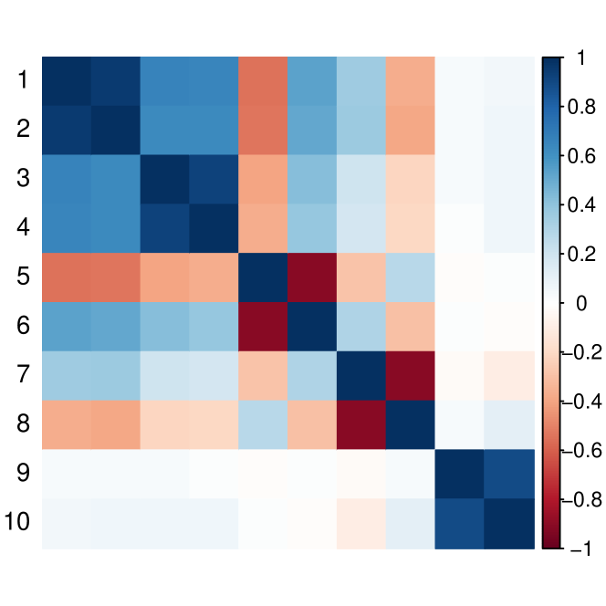
(a) $\delta=0$

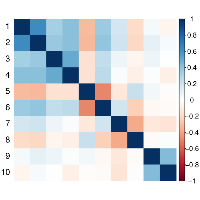
(b) $\delta=10$

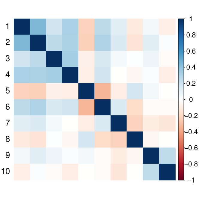
(c) $\delta=20$

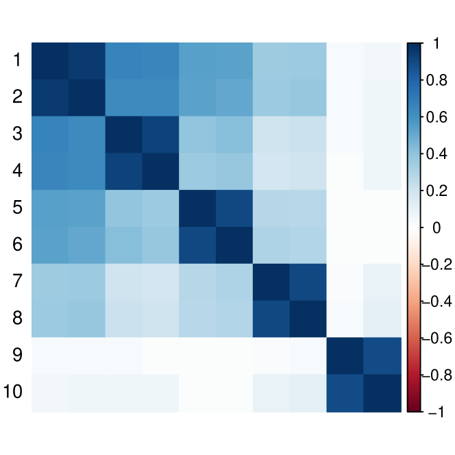
(d) $\delta=0$

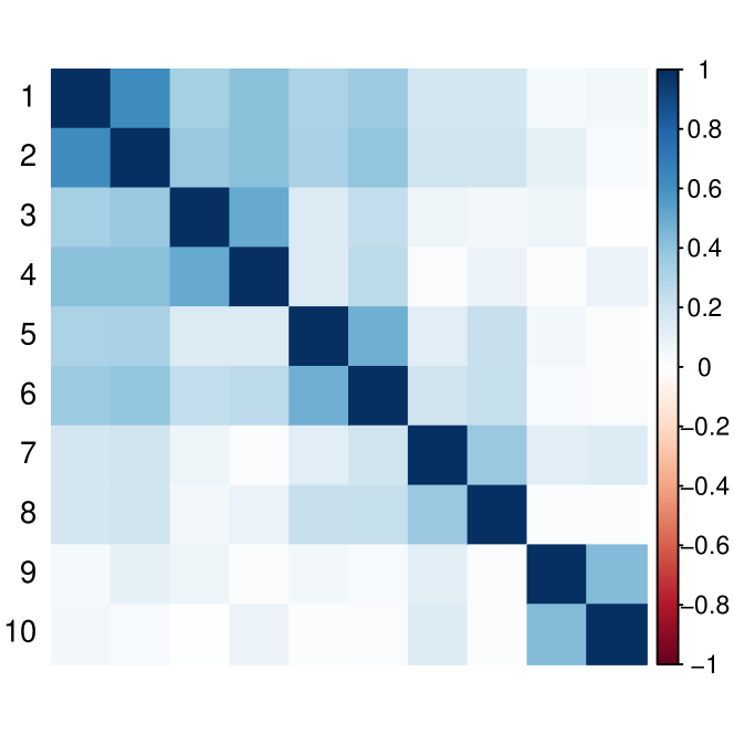
(e) $\delta=10$

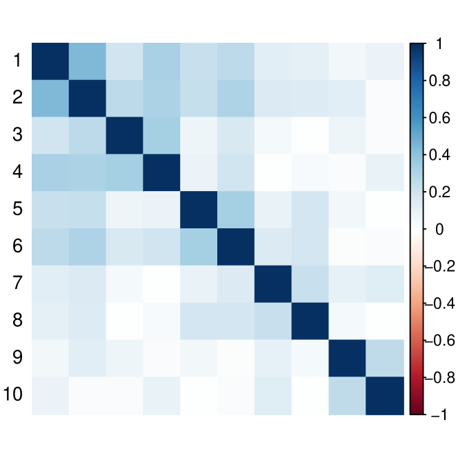
(f) $\delta=20$

Figure 1: Illustrative instances of simulated covariance matrices with six hierarchical groups, namely $(X_{1},X_{2})$, $(X_{3},X_{4})$, $(X_{5},X_{6})$, $(X_{7},X_{8})$, and $(X_{9},X_{10})$, with controlled deformation $\delta\in\{0,10,20\}$. The lower visualizations exhibit the covariance matrices presented in absolute values, enhancing the visualization of the hierarchical structure. Illustrations for $\delta\in\{5,15\}$ can be found in Supplementary Material 1.

We conduct a simulation study involving 1000 samples, where each sample contains $N=100$ observations drawn in accordance with equation (8). In addition to the inherent sample noise, we introduce a noise matrix that follows a $N(\bm{0},\delta\bm{I})$ distribution, with $\delta\in\{0,5,10,15,20\}$. The noise matrix is added to each sample. To ensure uniformity for comparison, we standardize each sample, resulting in the sample covariance matrix being equal to the sample correlation matrix. When $\delta$ is low, the generated data exhibit a hierarchical structure comprising six groups, each consisting of two strongly correlated variables. However, with an increase in $\delta$, the inter-group correlations decrease. For an illustrative representation, refer to Figure 1, which illustrates the covariance matrix for $\delta\in\{0,10,20\}$.

As explained in Section 3.1 and Algorithm 1, our approach to identifying the hierarchical block diagonal structure of the covariance matrix involves employing hard-thresholding sparse approximations of the singular vectors. The calculation of sparse loadings relies on a penalization parameter, denoted as $\theta$, while the hard-thresholding procedure is dependent on a specified cut-off value $\tau$.

Sparse loadings were calculated using the penalized matrix decomposition (PMD) introduced by Witten et al. (2009). In PMD, the penalization parameter $\theta$ is chosen within the range $[1,\sqrt{M}]$. A value of $\theta=1$ applies the strongest penalization, often resulting in unit vectors, while $\theta=\sqrt{M}$ imposes no penalization, producing singular vectors without enforced sparseness. We utilized a grid search approach to select the regularization and hard-thresholding parameters. The grid search involved exploring combinations of $(\theta,\tau)$ values from the cartesian product $\{1,1.1,1.2,\ldots,\sqrt{M}\}\times\{0,0.05,0.1,\ldots,0.5\}$. The aim was to identify the blocks with the largest dissimilarity.

We used the functions for the parameter tuning and for the block detection provided by the CRAN contributed package prinvars (Bauer and Holzapfel, 2023). These functions were specifically developed for this work and were used in the simulations. We compare the performance of our method with ICLUST (Revelle, 1979) which is aivailable in the CRAN contributed package psych (Revelle, 2023).

4.2 Simulation results

We calculated the accuracy of correctly detecting each group in the hierarchical structure for our proposed method using the four distinct linkage functions discussed in Section 3.2. For comparison, we also calculated the accuracy of the ICLUST method (Revelle, 1979). The objective was to sequentially detect $(X_{9},X_{10})$ first, followed by $(X_{8},X_{9})$, and so on, in the hierarchical arrangement. The outcomes of these analyses are visually presented in Figure 2, while precise numerical results can be found in Table LABEL:table:SimulationResults in A.

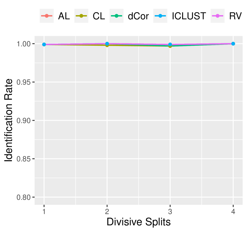
(a) $\delta=0$

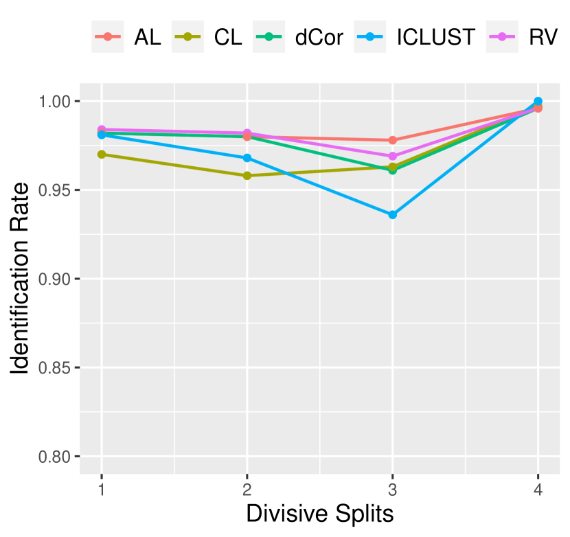
(b) $\delta=10$

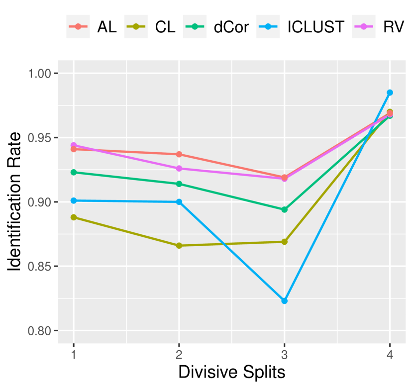
(c) $\delta=20$

Figure 2: Identification rates as a measure of accuracy for our method with linkage functions discussed in Section 3.2, and for the ICLUST method. The four splits of $(X_{9},X_{10})$, $(X_{7},X_{8})$, $(X_{5},X_{6})$, and $(X_{4},X_{5})$ needed to be detected in recursive order. The identification rate is illustrated for $\delta\in\{0,10,20\}$ and all numerical results are provided in Table LABEL:table:SimulationResults in A. Illustrations for $\delta\in\{5,15\}$ can be found in Supplementary Material 1.

In total, our proposed method for detecting distinct blocks and identifying the underlying hierarchical structure demonstrates a noteworthy level of accuracy. Complete linkage performs worse than the distance correlation, RV-coefficient, and average linkage, all of which yield similar outcomes. In contrast, the ICLUST method exhibits better performance relative to the complete linkage approach, albeit slightly trailing behind our proposed method using the remaining linkage functions. The identification rate decreases with $\delta$ for all approaches, however, it remains consistently high across the spectrum of analyzed values.

5 Example

In this section, we present the application of hierarchical variable clustering using SVD on the Bechtoldt sample (Thurstone and Thurstone, 1941; Bechtoldt, 1961) consisting of $M=17$ variables representing six mental ability tests: Memory (First Names, Word Number), Verbal (Sentences, Vocabulary, Completion), Words (First Letter, Four Letter Words, Suffixes), Space (Flags, Figures, Cards), Number (Addition, Multiplication, Three Higher), and Reasoning (Letter Series, Pedigrees, Letter Grouping).

The correlation matrix corresponding to the data is available in the CRAN contributed package psych (Revelle, 2023). We visualize the outcome using a dendrogram along with the sample covariance matrix in Figure 3(b). Based on the performance analysis in Section 4.2, we selected the average linkage function for the clustering procedure. The numerical dissimilarities calculated using the average linkage function are provided in Supplementary Material 2. For completeness, the dendrograms created with the other linkage functions can also be found in Supplementary Material 2, along with the dissimilarities calculated in each case.

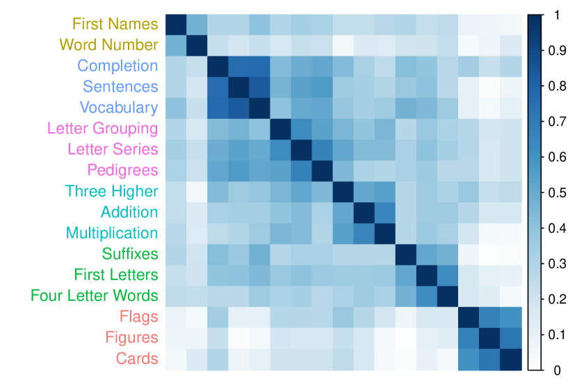
(a) Correlation matrix of the Bechtoldt sample

(b) Dendrogram using average linkage $d_{\mathrm{AL}}$

Figure 3: Correlation matrix of the Bechtoldt sample and the outcome of hierarchical variable clustering using SVD visualized as a dendrogram. The dendrogram illustrates the detection of the six mental abilities and provides the dissimilarity between these groups calculated using the average linkage function.

Hierarchical variable clustering using SVD reveals the hierarchical structure within and between the mental abilities. The dendrogram illustrates the detection of the six mental abilities: Space, Memory, Words, Number, Verbal, and Reasoning. The abilities are recursively split in descending order from left to right in the dendrogram. For example, Space is split first from the remaining mental abilities, while Verbal is closest to Reasoning and therefore split last.

Notably, there is no distinct horizontal cut-point for the dendrogram to separate the six mental abilities as different clusters. This is due to the high similarity of Verbal and Reasoning, and is illustrated in Figure 4. The results of hierarchical variable clustering using SVD therefore challenge the assumption of six different mental ability tests. Rather, we conclude that the tests contained in the sample test for five different abilities rather than six, where Verbal and Reasoning can be considered as one single mental ability due to their similarity.

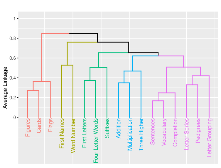
(a) Dendrogram with five groups

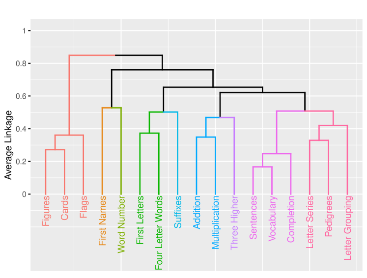
(b) Dendrogram with nine groups.

Figure 4: Dendrogram for the Bechtoldt sample with two different horizontal cut-points different numbers of groups. To split Verbal and Reasoning, a cut-point is needed that results in a total of nine groups.

6 Conclusion

In this research paper, we proposed a non-parametric approach for hierarchical variable clustering using SVD. Our method aims to identify the block diagonal structure of the covariance matrix using the singular vectors of the sample or the eigenvectors of the covariance matrix. We group variables based on their dissimilarity and we propose different linkage functions to assess the dissimilarity. We demonstrate the effectiveness of our approach through a simulation study and by applying it to a real data example. The results of our study contribute to the validation of the model and highlight its potential applications.

There are several possible directions for future research on our proposed model. First, more linkage functions could be evaluated to determine their effectiveness in identifying the hierarchical structure of variables. This would provide a more comprehensive understanding of the different approaches and their suitability for different types of data. Second, the method could be applied to evaluate the number of factors to be selected in factor analysis based on the number of clusters with a similar dissimilarity between them.

7 Supplementary Material

1. Supplementary illustrations corresponding to Figure 1 and Figure 2. Specifically addressing the scenario in which $\delta\in\{5,15\}$.

2. Extended results for the example in Section 5.

3. Code to replicate the simulations in Section 4 and the example in Section 5.

Appendix A Complementary Results

This section contains complementary results for the simulation study in Section 4. We provide the identification rates for our method using the four linkage functions discussed in Section 3.2, and for the ICLUST method (Revelle, 1979) in Table LABEL:table:SimulationResults.

Table 1: Numerical simulation results for the identification rate. We conducted ICLUST (Revelle, 1979) and hierarchical variable clustering using SVD using linkage functions based on the distance correlation ($d_{\mathrm{dCor}}$), RV-coefficient ($d_{\mathrm{RV}}$), complete linkage ($d_{\mathrm{CL}}$), and average linkage ($d_{\mathrm{AL}}$).

$\delta$	Block	$d_{\mathrm{dCor}}$	$d_{\mathrm{RV}}$	$d_{\mathrm{CL}}$	$d_{\mathrm{AL}}$	ICLUST
$\delta=0$	$(X_{9},X_{10})$	0.999	0.999	0.999	0.999	0.999
$\delta=0$	$(X_{7},X_{8})$	1.000	1.000	0.998	1.000	1.000
$\delta=0$	$(X_{5},X_{6})$	0.997	0.999	0.997	0.999	0.999
$\delta=0$	$(X_{3},X_{4})$	1.000	1.000	1.000	1.000	1.000
$\delta=5$	$(X_{9},X_{10})$	0.995	0.997	0.992	0.995	0.993
$\delta=5$	$(X_{7},X_{8})$	0.991	0.994	0.984	0.993	0.994
$\delta=5$	$(X_{5},X_{6})$	0.989	0.996	0.992	0.996	0.976
$\delta=5$	$(X_{3},X_{4})$	1.000	1.000	1.000	1.000	1.000
$\delta=10$	$(X_{9},X_{10})$	0.982	0.984	0.970	0.982	0.981
$\delta=10$	$(X_{7},X_{8})$	0.980	0.982	0.958	0.980	0.968
$\delta=10$	$(X_{5},X_{6})$	0.961	0.969	0.963	0.978	0.936
$\delta=10$	$(X_{3},X_{4})$	0.996	0.996	0.997	0.996	1.000
$\delta=15$	$(X_{9},X_{10})$	0.954	0.970	0.939	0.966	0.942
$\delta=15$	$(X_{7},X_{8})$	0.937	0.951	0.920	0.958	0.942
$\delta=15$	$(X_{5},X_{6})$	0.932	0.946	0.916	0.948	0.867
$\delta=15$	$(X_{3},X_{4})$	0.987	0.987	0.988	0.988	0.999
$\delta=20$	$(X_{9},X_{10})$	0.923	0.944	0.888	0.941	0.901
$\delta=20$	$(X_{7},X_{8})$	0.914	0.926	0.866	0.937	0.900
$\delta=20$	$(X_{5},X_{6})$	0.894	0.918	0.869	0.919	0.823
$\delta=20$	$(X_{3},X_{4})$	0.967	0.968	0.970	0.969	0.985

Table 1: Numerical simulation results for the identification rate. We conducted ICLUST (Revelle, 1979) and hierarchical variable clustering using SVD using linkage functions based on the distance correlation ($d_{\mathrm{dCor}}$), RV-coefficient ($d_{\mathrm{RV}}$), complete linkage ($d_{\mathrm{CL}}$), and average linkage ($d_{\mathrm{AL}}$). (continued).

References

- Bauer (2022) Bauer, J. O., 2022. Variable selection and covariance structure identification using sparse principal loading analysis. arXiv:2211.16155.
- Bauer and Drabant (2021) Bauer, J. O., Drabant, B., 2021. Principal loading analysis. J. Multivar. Anal. 184.
- Bauer and Holzapfel (2023) Bauer, J. O., Holzapfel, R., 2023. prinvars: Principal Variables. R package version 1.0.0.
- Bechtoldt (1961) Bechtoldt, H. P., 1961. An empirical study of the factor analysis stability hypothesis. Psychometrika 26, 405–432.
- Carroll (1993) Carroll, J. B., 1993. Human cognitive abilities: A survey of factor-analytic studies. Cambridge University Press, New York, NY, USA.
- Cavicchia and Vichi (2022) Cavicchia, C., Vichi, M., 2022. Second-order disjoint factor analysis. Psychometrika 87, 289–309.
- Cavicchia et al. (2020) Cavicchia, C., Vichi, M., Zaccaria, G., 2020. The ultrametric correlation matrix for modelling hierarchical latent concepts. AStA Adv. Stat. Anal. 14, 837–853.
- Cavicchia et al. (2022) Cavicchia, C., Vichi, M., Zaccaria, G., 2022. Hierarchical disjoint principal component analysis. AStA Adv. Stat. Anal.
- de Prado (2016) de Prado, M. L., 2016. Building diversified portfolios that outperform out of sample. J. Portf. Manag. 42 (4), 59–69.
- Digman (1990) Digman, J. M., 1990. Personality structure: Emergence of the five-factor model. Annu. Rev. Psychol. 41 (1), 417–440.
- Escoufier (1973) Escoufier, Y., 1973. Le traitement des variables vectorielles. Biometrics 29 (4), 751–760.
- Holzinger (1944) Holzinger, K. J., 1944. A simple method of factor analysis. Psychometrika 9, 257–262.
- Jöreskog (1969) Jöreskog, K. G., 1969. A general approach to confirmatory maximum-likelihood factor analysis. Psychometrika 34 (2), 183–202.
- Kaufman and Rousseeuw (1990) Kaufman, L., Rousseeuw, P. J., 1990. Finding Groups in Data: An Introduction to Cluster Analysis. Wiley, New York.
- Liu et al. (2012) Liu, X., Zhu, X.-H., Qiu, P., Chen, W., 2012. A correlation-matrix-based hierarchical clustering method for functional connectivity analysis. J. Neurosci. Methods 211 (1), 94–102.
- Mantegna (1999) Mantegna, R. N., 1999. Hierarchical structure in financial markets. Eur. Phys. J. B 11, 193–197.
- McGrew (2009) McGrew, K. S., 2009. Chc theory and the human cognitive abilities project: Standing on the shoulders of the giants of psychometric intelligence research. Intelligence 37 (1), 1–10.
- Plasse et al. (2007) Plasse, M., Niang, N., Saporta, G., Villeminot, A., Leblond, L., 2007. Combined use of association rules mining and clustering methods to find relevant links between binary rare attributes in a large data set. Comput. Stat. Data Anal. 52 (1), 596–613.
- R Core Team (2022) R Core Team, 2022. R: A Language and Environment for Statistical Computing. R Foundation for Statistical Computing, Vienna, Austria.
- Revelle (1979) Revelle, W., 1979. Hierarchical cluster analysis and the internal structure of tests. Multivar. Behav. Res. 14 (1), 57–74.
- Revelle (2023) Revelle, W., 2023. psych: Procedures for Psychological, Psychometric, and Personality Research. R package version 2.3.3.
- Robert and Escoufier (1976) Robert, P., Escoufier, Y., 1976. A unifying tool for linear multivariate statistical methods: The RV-coefficient. J. R. Stat. Soc. C 25 (3), 257–265.
- Shen and Huang (2008) Shen, H., Huang, J. Z., 2008. Sparse principal component analysis via regularized low rank matrix approximation. J. Multivar. Anal. 99 (6), 1015–1034.
- Soffritti (1999) Soffritti, G., 1999. Hierarchical clustering of variables: a comparison among strategies of analysis. Commun. Stat. Simul. Comput. 28 (4), 977–999.
- Székely et al. (2007) Székely, G. J., Rizzo, M. L., Bakirov, N. K., 2007. Measuring and testing dependence by correlation of distances. Ann. Stat. 35 (6), 2769–2794.
- Thurstone and Thurstone (1941) Thurstone, L. L., Thurstone, T. G., 1941. Factorial studies of intelligence. University of Chicago Press, Chicago.
- Vichi and Saporta (2009) Vichi, M., Saporta, G., 2009. Clustering and disjoint principal component analysis. Comput. Stat. Data Anal. 53 (8), 3194–3208.
- Vigneau and Qannari (2003) Vigneau, E., Qannari, E. M., 2003. Clustering of variables around latent components. Comm. Statist. Simulation Comput. 32 (4), 1131–1150.
- Witten et al. (2009) Witten, D. M., Tibshirani, R., Hastie, T. A., 2009. A penalized matrix decomposition, with applications to sparse principal components and canonical correlation analysis. Biostatistics 10 (3), 515–534.
- Yu et al. (2015) Yu, Y., Wang, T., Samworth, R. J., 2015. A useful variant of the Davis–Kahan theorem for statisticians. Biometrika 102 (2), 315–323.
- Zou et al. (2006) Zou, H., Hastie, T., Tibshirani, R., 2006. Sparse principal component analysis. J. Comp. Graph. Stat. 15 (2), 265–286.