Optimal strategies for kiiking: active pumping to invert a swing

Abstract

Kiiking is an extreme sport in which athletes alternate between standing and squatting to pump a stationary swing till it is inverted and completes a rotation. A minimal model of the sport may be cast in terms of the control of an actively driven pendulum of varying length to determine optimal strategies. We show that an optimal control perspective, subject to known biological constraints, yields time-optimal control strategy similar to a greedy algorithm that aims to maximize the potential energy gain at the end of every cycle. A reinforcement learning algorithms with a simple reward is consistent with the optimal control strategy. When accounting for air drag, our theoretical framework is quantitatively consistent with experimental observations while pointing to the ultimate limits of kiiking performance.

Introduction.

Sports offer a fertile playground for the interaction of physics, physiology and cognitive neuroscience, raising questions about how humans learn and execute extreme motor tasks, sometimes accompanied by fame and fortune. The playground swing offers a humble and familiar example: a child wiggles on it randomly at first, but soon learns to move their body rhythmically, leading to limited amplitudes, but unlimited pleasure! But how does an individual learn to swing? What are the optimal strategies for pumping a swing? And how do physical and biological constraints enter in constraining the solution? Here, we study an extreme version of this problem termed Kiiking, invented in Estonia [1]. An athlete strapped on a platform connected to an especially long ($\sim~{}7$ m) rigid swing (Estonian: kiik) made of rigid bars Fig. 1(a) pumps the swing by standing and squatting, with the goal of inverting the longest possible swing and completing a full rotation within the shortest time.

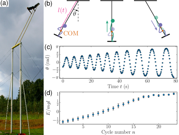
Figure 1: (a) An athlete on a tall kiiking swing. The arms of the swing are rigid, and the athlete is attached to the base by their feet. Adapted from Estonian Kiiking Association [2], ©2014 Estonian Kiiking Association. (b) A schematic of an athlete pumping the kiiking swing by squatting and standing. The swing-athlete system is modeled as a simple (point-mass) pendulum with variable length $l(t)$. Over the course of one cycle, the athlete quickly stands up when the swing is near its lowest point, and squats down as the swing reaches its highest point. This stand-squat cycle is repeated twice over each oscillation of the swing’s motion. (c) The angle $\theta$ measured from experiments [3] as a function of time for a successful kiiking attempt. The length of the swing is approximately $7\text{\,}\mathrm{m}\text{/}$. (d) Nondimensionalized energy $E/mgl_{0}\approx-\cos\theta$ after the $n$th cycle, i.e. at the $n$th extremum of $\theta$.

Swings can be minimally modeled as an active pendulum, driven by either leaning back and forth  [4, 5], or by standing and squatting [6]. In the linearized, small amplitude limit, the standing-squatting mode Fig. 1(a), modeled as a pendulum with time-varying length $l$, is a prototypical example of a parametrically driven oscillator [7, 8]. However, to properly understand kiiking from a neurophysical perspective requires one to go beyond this and address the nonlinear problem from the perspective of optimal strategies for modulating the length, and further how this might be learned. A step in this direction takes the perspective of optimal control theory and maximize the angle $\theta$ of the swing at its highest point over a half-period e.g. [9], or minimize the time needed to reach a given target angle or target potential energy [10, 11, 12, 13]. Assuming that the length $l$ can change discontinuously leads to the following intuitive result: stand up at the lowest point of the swing, and squat at the highest point. However, biological and physical constraints limit the rate at which any athlete can stand and squat, especially at higher angular speeds when fighting gravity. Here we combine the analysis of publicly available videos of kiiking [3, 14, 15, 16, 17] to extract time series, and use simple estimates of constraints on human athletic performance, e.g. maximum power exerted to constrain a minimal model of kiiking in terms of an extensible controllable pendulum.

Experimental data analysis.

In order to develop a quantitative understanding of kiiking strategies we found videos of kiiking online [1, 2] and took snapshots of the videos at a rate of 3 Hertz, which we analyzed using the Fiji software platform [18] to measure the angle the swing makes with the vertical, as shown in Figure 1(c) as the athlete makes a full swing up to 180^∘ (see SI SI). To estimate the speed and power limits on human performance, we note that athletes can squat/standup in about a second, consistent with the maximum rate of standing from the video data of about $140$ cm/s, and that the reported peak power output during a jump squat is on the order of 5000 W [19]. We use these estimates later to set simulation parameters as we search for optimal swinging strategies.

Mathematical model.

We model the kiiking system as a pendulum with a bob of mass $m$ connected to a pivot by a massless rigid rod of variable length $l$, with $l_{-}<l<l_{+}$, the bounds corresponding to squatting and standing, and $\theta$ the angle between the pendulum and the downward vertical direction Figure 1(b). Neglecting any motion of the center of mass perpendicular to the swing arms, as well as friction and air resistance for now, the kinetic and potential energy of the system are $T=\frac{1}{2}m\big{[}(l\dot{\theta})^{2}+\dot{l}^{2}\big{]}$ and $V=-mgl\cos\theta$ respectively. Defining the conjugate momentum $p=ml^{2}\dot{\theta}$, the evolution of the state $\mathbf{x}=(\theta,p,l)$ is given by Hamilton’s equations

$$\dot{\theta} =\frac{1}{ml^{2}}p,$$ (1)

$$\dot{p} =-mgl\sin\theta,$$

$$\dot{l} =u,$$

where $u$ is the rate of change of $l$, which we take as the control variable. We nondimensionalize the system (1) by choosing units so that $m=l_{0}=t_{0}=1$ where $l_{0}=(l_{+}+l_{-})/2$ is a characteristic length scale and $t_{0}=\sqrt{l_{0}/g}$ is a corresponding time scale. We write the nondimensionalized equations in the form

$$\begin{gathered}\dot{\mathbf{x}}=\mathbf{f}(\mathbf{x},u)=\mathbf{F}(\mathbf{x})+\mathbf{G}(\mathbf{x})u,\;\mathbf{x}(0)=\mathbf{x}_{0},\\ \mathbf{F}(\mathbf{x})=\begin{pmatrix}p/l^{2}\\ -l\sin\theta\\ 0\end{pmatrix},\quad\mathbf{G}(\mathbf{x})=\begin{pmatrix}0\\ 0\\ 1\end{pmatrix}\end{gathered}$$ (2)

to emphasize that the system is affine in the control $u$. For simplicity, we only consider initial conditions of the form $\mathbf{x}_{0}=(\theta_{0},0,l_{+})$ where $\theta_{0}\neq 0$.

Our goal is to find a control $u$ so that the system reaches the target set $S=\{(\theta,p,l)\mid\theta=\pm\pi\}$ in minimum time, subject to certain constraints on $u$ and the trajectory $\mathbf{x}(t)$, which will be detailed below. The control may be given in the form of an open-loop control $u=u(t)$, or else as a feedback control policy $u=\pi(\mathbf{x})$. Importantly, the bound $l_{-}\leq l\leq l_{+}$ means that, for most initial conditions, any control which steers the system to $S$ must involve several cycles of squatting followed by standing. These individual cycles will be analyzed first before turning to the full optimal control problem.

To gain some intuition about the system, we note that the rate of change of the (nondimensionalized) energy is

$$\dot{E}=u\dot{u}-(p^{2}/l^{3}+\cos\theta)u.$$ (3)

The first term vanishes over a cycle, so we consider only the second term. For the system to gain energy, we must take $u<0$ (corresponding to standing up) when the mass is near its lowest point, so that $p^{2}/l^{3}+\cos\theta$ is maximal. Conversely, we should take $u>0$ near the highest point in order to minimize energy losses during the squatting phase. In our chosen units, the minimum energy needed to reach the target set $S$ is simply $E=l_{-}$.

We make the natural assumption that the rate $u=\dot{l}$ at which the length of the pendulum can be changed is bounded by some maximum, $\lvert u\rvert\leq u_{m}$. Motivated by equation (3), we also impose a power bound of the form $-(p^{2}/l^{3}+\cos\theta)u\leq P_{m}$ for some $P_{m}>0$ . The two constraints imply that $u^{-}\leq u\leq u^{+}$ where

$$u^{\pm}=u^{\pm}(\mathbf{x})=\pm\min\big{(}u_{m},\frac{\mp P_{m}}{p^{2}/l^{3}+\cos\theta}\big{)}$$ (4)

Finally, we define the dimensionless parameter $\Delta l\coloneqq(l_{+}-l_{-})/2$ so that $l$ is bounded between $1-\Delta l$ and $1+\Delta l$. For kiiking athletes, typical ranges for the dimensionless parameters are $0.04\leq\Delta l\leq 0.08$, $0.1\leq u_{m}\leq 0.15$, and $0.1\leq P_{m}\leq 0.25$.

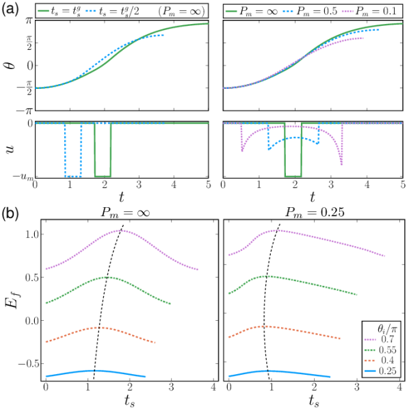
Figure 2: Analysis of the standing phase of a stand-squat cycle. Starting at the switching time $t=t_{s}$, the athlete decreases the swing length $l$ at the maximum rate $u=u^{-}$ (Eq. (4)) until $l$ reaches the minimum value $l_{-}$. (a) The angle $\theta$ and control $u=\dot{l}$ as functions of (nondimensionalized) time. Left: The switching time $t_{s}$ is varied in the absence of power constraints ($P_{m}=\infty$). The greedy switching time $t_{s}^{g}$ (solid green lines) maximizes the energy gained by the system. Right: Solutions with $t_{s}=t_{s}^{g}$ and varying power bounds $P_{m}$. In both cases, $\Delta l=0.115$, $u_{m}=0.5$. (b) Energy $E_{f}$ at the end of a cycle as a function of the switching time $t_{s}$. Each solid curve corresponds to a different initial angle $\theta_{i}=\theta(0)$. The dashed black curve indicates the greedy switching time $t_{s}^{g}$ for each $\theta_{i}$. For sufficiently large $P_{m}$, $t_{s}^{g}$ increases monotonically with $\theta_{i}$. Here, $\Delta l=0.05$, $u_{m}=0.1$.

Greedy control algorithm.

Figure 2 shows numerical solutions of equation (2) subject to the constraints $l_{-}\leq l\leq l_{+}$ and $u^{-}\leq u\leq u^{+}$ (see Eq. 4) for the standing phase of a single cycle. At $t=0$, the swing starts from rest at an initial angle $\theta_{i}$ and remains in the lowest position ($l=l_{+}$) until a switching time $t_{s}$, when $u$ is taken to be the minimum value allowed by the rate and power constraints, i.e. $u(t)=u^{-}$ where $u^{-}$ is defined in equation (4). This $u(t)$ is maintained until $l$ reaches the minimum length $l_{-}$, after which $u(t)$ is identically zero. In particular, $u(t)$ is piecewise constant in the absence of power constraints ($P_{m}=\infty$). Figure 2 (a) shows some representative solutions and the corresponding controls. The angle $\theta$ at the end of the standing phase, and thus the energy gained by the system, is seen to depend sensitively on the switching time $t_{s}$. The dependence of the final energy $E_{f}$ on the switching time is shown explicitly in Figure 2 (b). We denote by $t_{s}^{g}$ the greedy switching time, which maximizes the energy at the end of the standing phase. In the limiting cases $P_{m}\to\infty$, $u_{m}\to\infty$, the greedy switching time is precisely when $\theta=0$, i.e. when the swing reaches its lowest point. This is in agreement with previous results [13, 12]. Since the period of a pendulum increases with amplitude, $t_{s}^{g}$ increases monotonically with $\theta_{i}$ for sufficiently large $P_{m}$. In the power-constrained case, the dependence is more complicated due to a competing effect: As $\theta_{i}$ increases, the power constraint becomes more strict, leading to smaller $\lvert u\rvert$ and earlier switching times $t_{s}^{g}$.

The preceding discussion suggests a greedy control strategy, obtained by repeatedly switching between standing and squatting at the greedy switching times. Specifically, let $u(t)=u^{(i)}(t)$ for $t^{(i)}\leq t<t^{(i+1)}$ ($i=1,\ldots,N$) where the $u^{(i)}$ vary cyclically between the values $u=u^{-}$, $u=0$ and $u=u^{+}$, and the switching times $t^{(i)}$ are chosen greedily, i.e. in order to maximize the energy at the end of each stand-squat cycle. By construction, this strategy achieves the task of reaching $S$ in the fewest number of stand-squat cycles. Moreover, it approximates the behavior observed from kiiking athletes. As we will show, the time-optimal solution has the same structure as the greedy strategy, but with slightly different switching times. We will now precisely pose the time-optimal control problem.

Time-optimal control.

We say that a measurable function $u\colon{}_{+}\to U$, $U=[-u_{m},u_{m}]$, is an admissible control if $u$ and the corresponding state trajectory $\mathbf{x}$, solution of (1), satisfy the inequality constraints

$$g(\mathbf{x}(t),u(t))\geq 0,\quad\mathbf{h}(\mathbf{x}(t))\geq 0,$$ (5)

where

$$g(\mathbf{x},u)=P_{m}+(p^{2}/l^{3}+\cos\theta)u,\;\mathbf{h}(\mathbf{x})=\begin{pmatrix}l_{+}-l\\ l-l_{-}\end{pmatrix}.$$

Define the terminal time $t_{f}=t_{f}(u)$ as the first time that the corresponding trajectory $\mathbf{x}$ hits the target set $S=\{(\theta,p,l)\mid\theta=\pm\pi\}$. Then the time-optimal control problem (TOCP) for the kiiking system can be stated as follows: Given an initial state $\mathbf{x}_{0}$, find an admissible control $u\in\mathcal{U}$ which minimizes $t_{f}$ subject to the state constraints (5).

The presence of the pure state constraints, represented by $\mathbf{h}(\mathbf{x})$ in equation (5), makes this a difficult problem to solve by variational methods. A set of necessary conditions for a control-trajectory pair to solve the optimal control problem are provided by the Pontryagin Maximum Principle (PMP) for both mixed control-state inequality constraints as well as pure state constraints [21]. Defining the control Hamiltonian associated with the TOCP as

$$H(\mathbf{x},\bm{\lambda},u)=\bm{\lambda}\cdot(\mathbf{F}(\mathbf{x})+u\mathbf{G}(\mathbf{x})),$$

the time derivative of the constraint function $\mathbf{h}$ is

$$\mathbf{h}^{1}(\mathbf{x},u)=\nabla\mathbf{h}(\mathbf{x})\cdot\mathbf{f}(\mathbf{x},u)=(-u,u)^{T}$$

and we define the restricted control set

$$\begin{gathered}\tilde{U}(\mathbf{x})\coloneqq\{u\in U\mid g(\mathbf{x},u)\geq 0\text{ and }\\ h^{1}_{i}(\mathbf{x},u)\geq 0\text{ if }h_{i}(\mathbf{x})=0,\;i=1,2\}.\end{gathered}$$ (6)

The PMP states that if $u^{*}\colon[0,t_{f}]\to U$ is an optimal control and $\mathbf{x}^{*}$ is the corresponding trajectory, then there exists a nowhere vanishing function $\bm{\lambda}^{*}\colon[0,t_{f}]\to{}^{3}$ (the costate) so that at any time $t$ the function $u\mapsto H(\mathbf{x}^{*}(t),\bm{\lambda}^{*}(t),u)$ attains its maximum on the restricted control region $\tilde{U}(\mathbf{x}^{*}(t))$ at $u=u^{*}(t)$.

In our case, the control Hamiltonian $H(\mathbf{x},\bm{(}\lambda),u)=\bm{\lambda}\cdot\mathbf{F}(\mathbf{x})+u\lambda_{3}$ depends on $u$ only through the term $u\lambda_{3}$. The coefficient $\varphi(t)=\lambda_{3}(t)$ multiplying $u$ is called the switching function and determines the structure of the optimal control. On interior arcs, i.e. at times $t$ when the constraint $\mathbf{h}$ is inactive, the PMP states that $u^{*}(t)=u^{+}$ if $\varphi(t)>0$ and $u^{*}(t)=u^{-}$ if $\varphi(t)<0$. In other words, $u^{*}$ changes between the maximum and minimum value at switching times when $\varphi$ switches sign. This completely determines $u^{*}(t)$ on interior arcs unless a singular arc occurs, i.e. if $\varphi(t)$ vanishes on a nontrivial interval. We find that singular arcs do not appear in our problem, so we do not consider them further. A time interval $[t_{1},t_{2}]$ on which the constraint $\mathbf{h}$ is active is called a boundary arc and its endpoints $t_{1},t_{2}$ are called junction times. We see that in the interior of a boundary arc, we necessarily have $u^{*}(t)=0$.

Computing the costate $\bm{\lambda}$ (and thus the switching function) requires solving a difficult nonlinear multi-point boundary value problem. Alternately, we can use standard nonlinear programming methods to determine $u^{*}(t)$ in terms of the sequence of switching times and junction times after we transcribe the time-optimal control problem into a finite-dimensional optimization problem [22]. This approach requires an initial guess which is sufficiently close to the optimal switching times. Since the greedy algorithm described in the previous section is near-optimal, it provides a suitable initial guess. The computed optimal control was verified using a direct collocation method implemented in CasADi [23] (See SI SIII). The optimal control and corresponding $\theta(t)$ are shown in Figure 3 (black lines). As expected, the optimal control has the same structure as the greedy strategy, and differs only slightly in the switching and junction times.

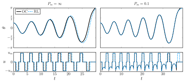
Figure 3: Time-optimal solution of the kiiking problem. The angle $\theta$ and control $u=\dot{l}$ as functions of (nondimensionalized) time for the numerically computed optimal control solution (OC, black lines) and the solutions obtained from reinforcement learning (RL, blue lines). Left: When the system is not power-constrained, the OC solution consists of several interior arcs where $u=\pm u_{m}$, separated by boundary arcs where $\lvert l-1\rvert=\Delta l$ and $u=0$. Right: In the presence of power constraints, $u$ takes the value $u^{\pm}$ (equation (4)) on the interior arcs. In both cases, the RL solution has the same form but with slightly different switching times. For both simulations, $\theta_{0}=\pi/4$, $\Delta l=0.05$, $u_{m}=0.1$.

Reinforcement learning.

Reinforcement learning (RL) provides an alternate approach to optimal decision and control problems [24]. While RL methods do not provide the same optimality guarantees as control theory methods, they are nevertheless very powerful as direct approaches, but need to phrased in terms of a state space $\mathcal{S}$, an action space $\mathcal{A}$, and a reward signal $\mathcal{R}$. For kiiking following the state space is given by Eq. 1, $S_{t}=(\theta_{t},p_{t},l_{t})$. Since the athletes must stand or squat as quickly as possible and otherwise do nothing, the action space is then $\mathcal{A}=\{-u_{m},0,u_{m}\}$, where $u_{m}$ is the maximum rate the athlete can stand or squat. At every time step the RL agent chooses an action and then follows the dynamics in equation 1, while ensuring that the power bounds are not exceeded at each time step.

To achieve the goal of training the agent to swing up to $\theta=\pi$ as quickly as possible, we supplement the time based reward with a reward which encourages incremental progress of the form

$$R_{t}=\begin{cases}1&\text{if }\theta=\pi\\ -1+E_{t}/E_{max}&\mathrm{otherwise}\end{cases}$$ (7)

where $E_{max}$ is the gravitational potential energy of the swing at $\theta=\pi$ and $E_{t}$ is the energy at time $t$. Energy increases as the swing cycles become larger in amplitude so an energy based reward is similar, but not identical, to a time based reward (see Fig 2). While using informative intermediate rewards via reward shaping is frequently used in RL problems [25], we found no improvement in performance after starting with the hybrid time-energy optimal agent and retraining it with the time based reward. As such we present results using the hybrid reward. Practically, we parameterized the policy as a neural network and use the Proximal Policy Optimization (PPO) [26] algorithm, a variant of traditional policy optimization, to update the network weights towards the optimal policy, and used the PPO implementation from Stable Baselines 3 [27], a thoroughly tested software package with implementations of various reinforcement learning algorithms (see SI SIII).

Figure 3 compares solutions obtained by the optimal control (OC)-based method to solutions found by the reinforcement learning (RL) algorithm (see also Videos 1-2 in the Supplemental Information). The solutions are identical apart from minor differences in switching and junction times. In particular, both solutions agree qualitatively with the general strategy of kiiking athletes, namely standing up as quickly as possible as $\theta$ passes through $0$ and squatting near zeros of $p$ (the extrema of $\theta$).

Comparison with data.

To validate our model, we compare the computed OC solutions to experimental data collected from trials by five different kiiking athletes [3, 14, 15, 16, 17]. In the absence of (mass and geometric) data on the athletes, it is not possible to directly compare $\theta(t)$ time series with our predictions, and so we compare the maximum scaled potential energy $E(n)$ at the end of each stand-squat cycle $n$, $E=-\cos\theta$. In figure 4 we see that for the longer trials, the $E(n)$ curves have a distinctive sigmoidal shape. Recalling equation (3), we see that the energy gain is initially limited by the small term $(p^{2}/l^{3}+\cos\theta)u\approx p^{2}u$, but at larger velocities, air resistance becomes non-negligible, and the $E(n)$ curve levels off. To capture these qualitative features, we modify our model Eq. (1) by adding a quadratic drag term $\dot{p}=-l\sin\theta-d\lvert p\rvert p/l,$ where $d$ is a dimensionless constant. Figure 4 shows the corresponding $E(n)$ using this form of the energy, for a challenging kiiking exercise requiring over twenty stand-squat cycles and captures the sigmoidal shape seen in data.

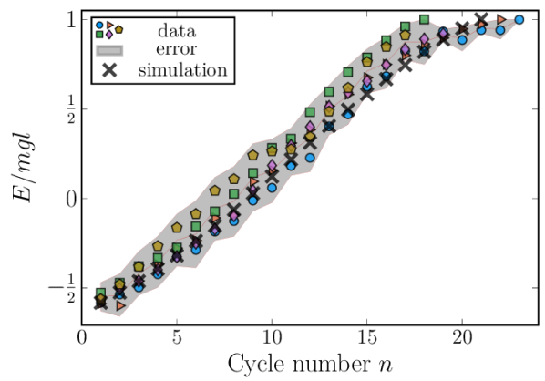
Figure 4: Nondimensionalized energy $E/mgl$ at the end of each stand-squat cycle for five trials by different kiiking trials. The gray ribbon shows the envelope of the error bars for all five trials. In the two longest trials (circles and triangles) the length of the swing arms is approximately $7\text{\,}\mathrm{m}\text{/}$. For the other trials, the length is smaller but not precisely known. Two of the series (diamonds and pentagons) show failed attempts, which ended without reaching $\theta=\pi$. A simulation with parameters $\Delta l=0.05$, $u_{m}=0.125$, $P_{m}=0.125$, $d=$2.75\text{\cdot}{10}^{-2}$$ is shown for comparison, and captures the sigmoidal shape of the $E(n)$ curves.

We note that adding the effects of air drag also has a qualitative implication for kiiking, i.e. for some parameter values, the set $S$ cannot be reached in finite time. To see this, we note that for given $u_{m},\Delta l,d>0$ there is, intuitively, a minimum power $P_{m}$ needed to complete the kiiking task. Furthermore, there is also a maximum swing length (minimum $\Delta l$) set by $u_{m},d$ above which the problem is infeasible for every $P_{m}>0$. In other words, there is a theoretical maximum swing length that a given athlete can use to successfully complete the kiiking task, regardless of the maximum power (see SI SIV).

Discussion.

Inspired by the humble swing and the extreme Estonian sport of kiiking, we considered the dynamics of an actively pumped pendulum. Using various approaches derived from control and learning theory, we computed strategies for the feedforward (open-loop) control of the swing and how an athlete or a robot might learn to complete the kiiking task from repeated attempts. Our results are consistent with observations of experimental data and serve to highlight the role of explicitly including physiological limitations on dynamics and energetics. Beyond the specific study, our work points to how even seemingly simple problems in physics. e.g. the playground swing, can be a rich source of new questions that link physics, physiology and neuroscience, when approached from a constrained learning perspective.

References

- Estonian Kiiking Association [2013] Estonian Kiiking Association, Eesti kiikinguliit, https://www.youtube.com/@EestiKiikingiLiit (2013), accessed: 01-10-23.
- Estonian Kiiking Association [2014a] Estonian Kiiking Association, Kiiking, https://commons.wikimedia.org/wiki/File:Kiiking_07.JPG (2014a), accessed: 01-10-23.
- Estonian Kiiking Association [2014b] Estonian Kiiking Association, Kaspar taimsoo, https://www.youtube.com/watch?v=Tz5UJX7N26s (2014b), accessed: 01-10-23.
- Case and Swanson [1990] W. B. Case and M. A. Swanson, The pumping of a swing from the seated position, American Journal of Physics 58, 463 (1990).
- Case [1996] W. B. Case, The pumping of a swing from the standing position, American Journal of Physics 64, 215 (1996).
- Wirkus et al. [1998] S. Wirkus, R. Rand, and A. Ruina, How to pump a swing, The College Mathematics Journal 29, 266 (1998).
- Burns [1970] J. A. Burns, More on pumping a swing, American Journal of Physics 38, 920 (1970).
- Berry [2018] M. Berry, Pumping a swing revisited: minimal model for parametric resonance via matrix products, European Journal of Physics 39, 055007 (2018).
- Lavrovskii and Formal’skii [1993] E. Lavrovskii and A. Formal’skii, Optimal control of the pumping and damping of a swing, Journal of Applied Mathematics and Mechanics 57, 311 (1993).
- Piccoli [1995] B. Piccoli, Time-optimal control problems for the swing and the ski, International Journal of Control 62, 1409 (1995).
- Kulkarni [2003] J. E. Kulkarni, Time-optimal control of a swing, in 42nd IEEE International Conference on Decision and Control (IEEE Cat. No. 03CH37475), Vol. 2 (IEEE, 2003) pp. 1729–1733.
- Piccoli and Kulkarni [2005] B. Piccoli and J. Kulkarni, Pumping a swing by standing and squatting: do children pump time optimally?, IEEE Control Systems Magazine 25, 48 (2005).
- Luo and Lee [1998] J. Luo and E. Lee, Time-optimal control of the swing using impulse control actions, in Proceedings of the 1998 American Control Conference. ACC (IEEE Cat. No. 98CH36207), Vol. 1 (IEEE, 1998) pp. 200–204.
- Estonian Kiiking Association [2014c] Estonian Kiiking Association, Ants tamme, https://www.youtube.com/watch?v=khGZLFHmqz0 (2014c), accessed: 01-10-23.
- Caters Video [2022] Caters Video, Woman daringly swings in full circle while kiiking, https://www.youtube.com/watch?v=FZ4O09AFzDw (2022), accessed: 01-10-23.
- KiikingTeam [2011a] KiikingTeam, Daniel kiiking record attempt (fail), https://www.youtube.com/watch?v=N4VJx_B1Cfo (2011a), accessed: 01-10-23.
- KiikingTeam [2011b] KiikingTeam, Jake kiiking record attempt (fail), https://www.youtube.com/watch?v=FDvtODCUrkk (2011b), accessed: 01-10-23.
- Schindelin et al. [2012] J. Schindelin, I. Arganda-Carreras, E. Frise, and et al, Fiji: an open-source platform for biological-image analysis., Nature Methods 9, 676 (2012).
- Cormie et al. [2007] P. Cormie, R. Deane, and J. M. McBride, Methodological concerns for determining power output in the jump squat, The Journal of Strength & Conditioning Research 21, 424 (2007).
- Note [1] Note that this bound does not take into account the contribution to . This is done for the sake of simplicity; however, this term is usually small compared to the other two terms when the constraint is active, except on very short times when almost has a jump-like discontinuity.
- Sethi [2021] S. P. Sethi, The maximum principle: Pure state and mixed inequality constraints, in Optimal Control Theory: Applications to Management Science and Economics (Springer International Publishing, 2021) pp. 115–144.
- Maurer and Vossen [2009] H. Maurer and G. Vossen, Sufficient conditions and sensitivity analysis for optimal bang-bang control problems with state constraints, in System Modeling and Optimization: 23rd IFIP TC 7 Conference, Cracow, Poland, July 23-27, 2007, Revised Selected Papers 23 (Springer, 2009) pp. 82–99.
- Andersson et al. [2019] J. A. E. Andersson, J. Gillis, G. Horn, J. B. Rawlings, and M. Diehl, CasADi – A software framework for nonlinear optimization and optimal control, Mathematical Programming Computation 11, 1 (2019).
- Sutton and Barto [2018] R. S. Sutton and A. G. Barto, Reinforcement learning: An introduction 2nd Ed. (MIT Press Ltd, 2018).
- Ng et al. [1999] A. Y. Ng, D. Harada, and S. Russell, Policy invariance under reward transformations: Theory and application to reward shaping, in ICML, Vol. 99 (Citeseer, 1999) pp. 278–287.
- Schulman et al. [2017] J. Schulman, F. Wolski, P. Dhariwal, A. Radford, and O. Klimov, Proximal policy optimization algorithms (2017).
- Raffin et al. [2021] A. Raffin, A. Hill, A. Gleave, A. Kanervisto, M. Ernestus, and N. Dormann, Stable-baselines3: Reliable reinforcement learning implementations, Journal of Machine Learning Research 22, 1 (2021).