Forces inside a strongly-coupled scalar nucleon
Abstract
We investigate the gravitational form factors of a strongly coupled scalar theory that mimic the interaction between the nucleon and the pion. The non-perturbative calculation is based on the light-front Hamiltonian formalism. We renormalize the energy-momentum tensor with a Fock sector dependent scheme. We also systematically analyze the Lorentz structure of the energy-momentum tensor and identify the suitable hadron matrix elements to extract the form factors, avoiding the contamination of spurious contributions. We verify that the extracted form factors obey momentum conservation as well as the mechanical stability condition. From the gravitational form factors, we compute the energy and pressure distributions of the system. Furthermore, we show that utilizing the Hamiltonian eigenvalue equation, the off-diagonal Fock sector contributions from the interaction term can be converted to diagonal Fock sector contributions, yielding a systematic non-perturbative light-front wave function representation of the energies and forces inside the system.
I Introduction
One of the biggest mysteries in physics is the nature of the strong force that holds the quarks together inside the nucleons. This force is responsible for quark confinement, gluon binding, and 99% of the nucleon mass. The hadronic energy-momentum tensor (EMT) is a direct probe of how the force is distributed inside the hadrons, and has sparked renewed interest in recent research. For recent reviews, see Refs. Polyakov:2018zvc ; Burkert:2023wzr .
By virtue of the Lorentz symmetry, the hadron matrix element of the EMT of the nucleon (spin-1/2) can be parametrized by the gravitational form factors (GFFs) Kobzarev:1962wt ; Pagels:1966zza ,
| (1) |
where, , , , and is the hadron mass. The Lorentz scalars , and encode the information about the energy, momentum and stress distributions inside the hadrons. Similarly, for scalar hadrons (spin-0), the hadron matrix elements of the EMT can be written as Polyakov:2018zvc ,
| (2) |
The GFFs and exist for particles of all spins.
The term is associated with the stress component of the EMT, which reveals the mechanical properties of the nucleons. However, this form factor remains poorly understood. In fact, the term is dubbed as “the last global unknown” Polyakov:2018zvc . Unlike other GFFs, the value of the term at zero-momentum transfer is not fixed by global conservation laws. It depends on the internal QCD dynamics. Based on mechanical stability, Polyakov et al. conjectured that should be negative Perevalova:2016dln . This is supported by various model calculations Polyakov:2018zvc ; Ji:1997gm ; Petrov:1998kf ; Polyakov:1998ze ; Polyakov:2002yz ; Guzey:2005ba ; Cebulla:2007ei ; Pasquini:2007xz ; Hwang:2007tb ; Mai:2012yc ; Mai:2012cx ; Jung:2013bya ; Cantara:2015sna ; Hudson:2017oul ; Polyakov:2018exb ; Chakrabarti:2020kdc ; Metz:2021lqv ; Mamo:2022eui ; More:2021stk ; Fujita:2022jus ; GarciaMartin-Caro:2023klo ; More:2023pcy ; Freese:2022jlu ; Amor-Quiroz:2023rke ; Chakrabarti:2023djs . However, Ji and Liu argued that is positive for the hydrogen atom, a stable system Ji:2021mfb . The term also contributes to the anomalous mass of the proton, which probes the gluon distribution inside the nucleons Ji:1994av (cf. Lorce:2018egm ; Lorce:2021xku ; Burkert:2023wzr ). The term of the vacuum state gives the cosmological constant Teryaev:2013qba .
In the parton picture, the term contributes to the generalized parton distributions (GPDs) in the off-forward region Polyakov:2002yz ; Ji:1996nm , which provide the experimental access to the term. Burkert et al. extracted the force distributions inside the proton from the deeply virtual Compton scattering data collected at Jefferson lab Burkert:2018bqq ; Burkert:2021ith . However, the result has large systematic uncertainty and model dependence, due to the limited energy and luminosity of the experiment Kumericki:2019ddg ; Dutrieux:2021nlz . These measurements are expected to be significantly improved with the advent of electron ion colliders (EICs) Accardi:2012qut ; Anderle:2021wcy ; Accardi:2023chb . In the time-like region, the term can also be extracted from the two-photon production of the particle-antiparticle pair, as shown by Kumano et al. Kumano:2017lhr . Kharzeev proposed to use the near-threshold quarkonium photo-production to extract the anomalous mass Kharzeev:2021qkd . The nucleon term is also extracted from Lattice QCD Shanahan:2018nnv ; Hackett:2023nkr and a light-cone sum rule approach Anikin:2019kwi .
The term has been extensively investigated in perturbation theory, e.g. QCD at large momentum transfer Tong:2022zax . However, calculations with non-perturbative couplings are scarce. The force distribution has also been explored in phenomenological models Petrov:1998kf ; Polyakov:1998ze ; Polyakov:2002yz ; Guzey:2005ba ; Cebulla:2007ei ; Pasquini:2007xz ; Hwang:2007tb ; Mai:2012yc ; Mai:2012cx ; Jung:2013bya ; Cantara:2015sna ; Hudson:2017oul ; Polyakov:2018exb ; Chakrabarti:2020kdc ; Metz:2021lqv ; Mamo:2022eui ; More:2021stk ; Fujita:2022jus ; GarciaMartin-Caro:2023klo ; More:2023pcy ; Freese:2022jlu ; Amor-Quiroz:2023rke ; Chakrabarti:2023djs , such as holography Mamo:2022eui ; Fujita:2022jus , light-front quark-diquark model Chakrabarti:2020kdc , and Dyson-Schwinger equations with contact interaction Xing:2022mvk . One of the challenges of computing the term is that the stress component of the EMT involves the interaction, which needs to be properly renormalized and consistent with the dynamical solution of the hadron state. Otherwise, the extracted term may have unphysical divergences, as reported in prior work Chakrabarti:2020kdc .
Light-front quantization is a natural framework to investigate the structures of the hadrons in the non-perturbative regime Brodsky:1997de ; Bakker:2013cea ; Gross:2022hyw . It is the native language for parton physics, which describes how the hadrons are seen in modern high energy scattering experiments Feynman:1969ej ; Kogut:1972di ; Brodsky:1981rp . The spatial distribution of hadrons is only meaningful on the light front Miller:2010nz . This approach is closely related to physics in the infinite momentum frame Ji:2021znw . Furthermore, it also offers a systematic non-perturbative framework to tackle the strong interaction based on the Hamiltonian formalism Brodsky:1997de . Remarkable progress has been made in recent years with the development of theoretical methods and the increase of the computational power Gross:2022hyw ; Li:2015zah ; Xu:2022abw ; Kreshchuk:2020aiq ; Qian:2021jxp ; Vary:2016ccz . One of the core quantities in light-front quantization is the light-front wave function (LFWF), which encodes the full quantum information of the system Brodsky:1997de . The LFWF representation has been crucial in the investigation of the GFFs and . For instance, this representation provides a non-perturbative derivation of the absence of the anomalous gravitomagnetic moment, i.e. Brodsky:2000ii , where .
In non-relativistic quantum many-body theory, the quantum stress can be expressed as the virial using quantum many-body wave functions Godfrey:1988 ; Rogers:2001 . It is natural to expect that such a formulation can be generalized to quantum field theories (QFTs) using LFWFs. One of the main challenges in QFT is the involvement of the interaction terms in the EMT, which change the particle numbers and generate non-diagonal contributions within the Fock space.It has been posited that a LFWF representation of the term is not useful unless the full set of LFWFs was obtained Polyakov:2018zvc . Indeed, in phenomenological models, only the lowest Fock sectors111Quite often, only the valence sector is retained. See Refs. Lan:2021wok ; Xu:2022abw ; Pasquini:2023aaf for recent progress in incorporating higher Fock sector contributions. are available, and the effective quark-antiquark interactions are used. The interaction part of the EMT is effectively neglected.
In this work, we investigate the GFFs and in a strong-coupling scalar theory. The theory is one of the simplest yet nontrivial QFTs. It can be used to model the low-energy interaction of the (mock) nucleon and the (mock) pion. This theory is used to illustrate the properties of the term and its relation to GPDs based leading-order perturbative calculation Pobylitsa:2002vw ; Polyakov:1999gs . It is interesting to see how the forces inside the mock nucleon evolve as the coupling increases. This theory can be systematically renormalized using Fock sector dependent renormalization (FSDR) developed by Karmanov et al. Karmanov:2008br , which ensures the cancellation of the UV divergences even in the strong coupling regime. The eigenstate in the one-nucleon system is obtained in the light front Hamiltonian approach up to 4 particles (one mock nucleon plus three mock pions), where the Fock sector convergence is achieved Karmanov:2016yzu ; Li:2015iaw . This theory serves as an ideal playground for exploring the properties of the EMT in the non-perturbative regime. We evaluate the hadron matrix elements of the EMT and extract the GFFs. The EMT is renormalized with FSDR. From these results, we also obtain a general LFWF representation of the term, independent of the interaction details.
The rest of this work is organized as follows. In Sect. II, we introduce the light-front Hamiltonian formalism and set up the basic framework for the calculation. In Sect. III, we compute the hadron matrix elements of the EMT. In Sect. IV, we first analyze the covariant structure of the hadron matrix elements using covariant light-front dynamics (CLFD) Carbonell:1998rj . Based on these analyses and the expressions obtained in Sect. III, we extract the GFFs and and present their numerical results. In Sect. V, we further analyze the hadron matrix elements using the LFWF representation. In the forward limit (), momentum conservations and the Hamiltonian dynamics lead to well-known constraints on the GFFs. In the off-forward limit (), we derive a general LFWF representation for the term as well as the term. Finally, we conclude in Sect. VI. Some technical details are given in the Appendix.
II Light-front Hamiltonian formalism
The Lagrangian of the theory reads,
| (3) |
Here, and are the bare masses of the complex scalar field (mock nucleon) and real scalar field (mock pion), respectively. The physical masses are taken to be the nucleon mass and the pion mass , respectively. is the bare coupling. We also introduce a dimensionless coupling, , where is the physical coupling, is the physical mass of the mock nucleon. In the semi-classical limit, this theory describes a Yukawa type interaction with the coupling strength .
To simplify our calculations, we quench the theory, i.e., we neglect the contributions of nucleon-antinucleon loops, which would otherwise destabilize the vacuum Gross:2001ha . This approximation is justified by the large mass gap between the nucleons and the pions, which suppresses the pair creation effects. It is useful to introduce the mass counterterm: . In the quenched theory, the mock pion mass is not renormalized, viz. . The Fock space is built with Fock particles with the physical masses. N.B. we do not renormalize the fields, but instead normalize the state vector. The bare parameters are determined in FSDR Karmanov:2016yzu ; Li:2015iaw .
The EMT can be obtained as a Noether current of the translational symmetry222Note that for this simple scalar theory, the EMT is symmetric.,
| (4) |
Note that the EMT contains the bare parameters and needs to be renormalized. We adopt the same sector dependent bare parameters determined in FSDR. We quantize the theory on the light front , and the light-front Hamiltonian is obtained as the conserved charge of Dirac:1949cp ,
| (5) |
Here, the light-front component of a 4-vector is defined as,
| (6) |
In particular, is the light-front time and is the light-front energy. The integration measure is defined as .
At the initial time , the field operators can be expanded in terms of the creation and annihilation operators,
| (7) | ||||
| (8) |
The creation and annihilation operators obey the canonical commutation relations,
| (9) |
The state vectors of the physical particles are the solutions of the light-front Schrödinger equation,
| (10) |
In this work, we consider the one-nucleon sector, i.e., the mock nucleon dressed by mock pions. The mass eigenvalue is simply the physical nucleon mass . The state vector can be expressed in the Fock space,
| (11) |
where, is the -body phase space measure. is called the LFWF, which only depends on the longitudinal momentum fractions and the relative transverse momenta . And is the -body Fock state. Each Fock particle is on their mass shell: . The state vector is normalized as . Consequently, the LFWFs are normalized to unity,
| (12) |
It is useful to introduce the vertex functions , where, is the invariant mass squared of the Fock sector. It can be shown that the vertex function is the matrix element of the matrix,
| (13) |
Using the vertex functions, we can generalize the light-cone perturbation theory to the non-perturbative regime Weinberg:1966jm ; Karmanov:1976iv ; Carbonell:1998rj .
The theory is super-renormalizable. However, ultraviolet divergence does exist in loop integrals. We introduce the Pauli-Villars degree of freedom to regularize the divergence prior to renormalizing the theory. After a successful renormalization of the EMT operator, the GFFs are independent of the Pauli-Villars mass, as expected for the conserved current. We will suppress the Pauli-Villars regularization throughout. In Ref. Li:2015iaw , the theory is solved in the one-nucleon system up to 4 particles (1 mock nucleon plus 3 mock pions). By comparing with the solution from the three-body truncation Karmanov:2008br ; Karmanov:2016yzu , the Fock sector expansion is shown to converge up to the three-body truncations for the field strength renormalization constant as well as the electromagnetic form factor up to non-perturbative couplings. In this work, we adopt the three-body truncation to compute the GFFs.
III Hadron matrix elements
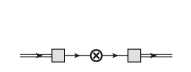
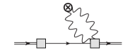
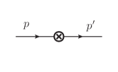
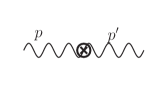
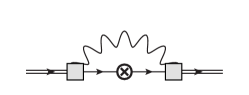
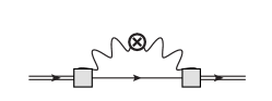
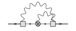
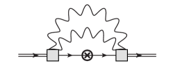
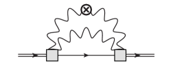
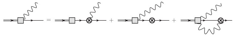
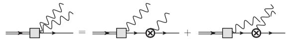
With the LFWFs solved from the light-front Schrödinger equation (10), we can compute the hadron matrix elements of the EMT using Eqs. (7–9, 11 & 4). The calculation can be neatly represented using light-front time-ordered diagrams as shown in Fig. 1. See Ref. Brodsky:1997de for a summary of the old-fashioned diagrammatic rules for light-front dynamics, also known as the Weinberg rules Weinberg:1966jm . The rules for the interaction vertices associated with the EMT can be obtained from the operator expression (4), as shown in Fig. 2. These rules are generalized to the non-perturbative regime by adopting the vertex functions for the hadron vertices Karmanov:1976iv ; Carbonell:1998rj . It is useful to introduce kinematical variables and . We also adopt the Drell-Yan frame to evaluate the hadron matrix elements, which dramatically simplify the algebra Drell:1969km .

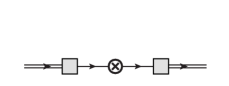
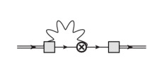
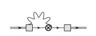
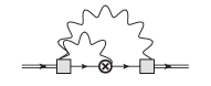
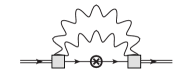
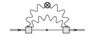
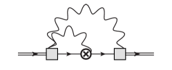
As we mentioned, the EMT contains counterterms. We adopt the FSDR scheme and assign the counterterms according to the Fock sector in which they reside. The values of the counterterms were obtained from solving the Schrödinger equation in the previous work Li:2015iaw ; Karmanov:2016yzu . These counterterms are sufficient to renormalize the EMT. To see this point, let us first see an example. Consider diagrams (a) & (b), as shown in Fig. 3. The corresponding expressions are,
| (14) | ||||
| (15) |
Here, is the one-body normalization constant. contains a mass counterterm . Compare with the self-energy function within the 3-body truncation,
| (16) |
We obtain,
| (17) |
as expected. Therefore, cancels out the mass counterterm contribution in diagram (a),
| (18) |
We collect the result of each diagram as follows.
III.1 Diagram (c)
III.2 Diagram (d)
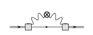
III.3 Diagram (e)
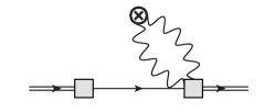
The relevant diagram is shown in Fig. 6. In the Drell-Yan frame , this diagram and its complex conjugate (denoted as ) vanish, .
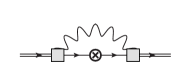
III.4 Diagram (f)
The relevant diagram is shown in Fig. 7.
| (33) |
A related diagram, (), is the Hermitian conjugate of diagram (f), as shown in Fig. 8,
| (34) |
III.5 Diagram (g)
III.6 Diagram (h)
III.7 Forward limit
To see the renormalization of the EMT, let us first examine the hadron matrix elements in the forward limit (). As we will see later in Sect. IV, to extract the GFFs, it is sufficient to consider and .
In the LFWF representation, , where is the probability of the one-body Fock sector. On the other hand,
| (49) | ||||
| (50) |
Hence, in the forward limit,
| (51) |
where,
| (52) |
is the two-body normalization constant. Similarly, one obtains, , where,
| (53) |
is the three-body normalization constant. Note that . Therefore, in the forward limit,
| (54) |
Here, we have used the normalization condition for the three-body truncation, .
Next, let us consider . This hadron matrix element is more complicated since it involves the interaction. The one-body part of is:
| (55) |
For the 2-body part, let us first consider the kinematical contribution, viz. excluding terms proportional to ,
| (56) |
Similarly, the 3-body kinematical contributions:
| (57) |
Next, let us consider the interacting terms, viz. all terms proportional to , in the forward limit. These involve diagrams . Note that the parts of and cancel out. The two-body interacting contribution, reads:
| (58) |
The expression in the curly bracket can be simplified using the equation of motion as shown in Fig. 11:
| (59) |
Hence, Eq. (58) becomes,
| (60) |
The full 2-body contribution becomes,
| (61) |
Finally, the only 3-body contribution of the interacting part is ,
| (62) | ||||
| (63) |
Again, applying the equation of motion (Fig. 12), the expression in the curly bracket becomes,
| (64) |
The interacting part of diagram- is,
| (65) |
Therefore, the full 3-body contribution is,
| (66) |
Summing over all three Fock sector contributions, the full EMT is,
| (67) |
As one can see, the hadron matrix elements do not depend on any counterterms, nor do they contain any additional divergence.
IV Gravitational form factors
IV.1 Covariant light-front dynamics
By virtue of the Lorentz symmetry, the hadron matrix elements of the EMT for a scalar particle can be parametrized by 2 GFFs,
| (68) |
where, and . In practical non-perturbative calculations, including those on the light front, however, the full Lorentz symmetry can only be retained in the exact continuum limit. As we impose truncations and approximations (e.g., neglecting higher Fock sectors), the dynamical symmetries, i.e. symmetries involving interactions, are likely to be broken and only the kinematical symmetries are manifest. As a result, the hadron matrix element of the EMT has to be reparametrized with the reduced symmetries Carbonell:1998rj .
In CLFD, this can be systematically constructed by introducing a null vector , which indicates the orientation of the quantization surface, the light front Carbonell:1998rj . Effectively, the state vector depends on . The standard light-front coordinate is recovered by choosing , viz. . Note that since the null vector is only defined up to a scaling factor, the dependence on is always in the form .
In CLFD, the form factors are complex functions of two Lorentz scalars, and . Hermiticity of the EMT operator implies . In the Drell-Yan frame Drell:1969km , the form factors become real functions. In this frame, the most general Lorentz structures of the hadron matrix element read,
| (69) |
where, and . The new GFFs are the spurious form factors. They are expected to vanish in the continuum limit when the full dynamics is incorporated. To extract the GFFs, we can compute the components of the EMT as follows.
| (70) | |||
| (71) | |||
| (72) | |||
| (73) | |||
| (74) | |||
| (75) |
Further simplification can be achieved by taking the Breit frame, ,
| (76) | |||
| (77) | |||
| (78) | |||
| (79) | |||
| (80) | |||
| (81) | |||
| (82) | |||
| (83) |
From these analyses, the term can be extracted from , while the term can be extracted from ,
| (84) | ||||
| (85) |
Note that the popular choice , the transverse stress tensor, is contaminated by the spurious GFF . Using these components to extract the term is not reliable, unless a proper combination is used Chakrabarti:2020kdc .
IV.2 Physical densities
From these two GFFs, we can compute several physical densities. These physical densities attain the same physical interpretation as those in classical field theory Li:2023 ,
| (86) |
Here, is the proper energy density. is the pressure, trace part of the stress tensor. Both quantities are Lorentz invariants. is the (traceless) shear tensor. The energy density is defined as Li:2023 ,
| (87) |
Note that the energy density is different from the Fourier transform of . Similarly, the pressure is Li:2023 ,
| (88) |
The shear tensor is also related to the term.
Another quantity of interest is the trace of the EMT , which is related to the anomalous mass in the proton. The trace density is,
| (89) |
As a comparison, the Fourier transform of in the Breit frame is,
| (90) |
The trace of the light-front EMT gives rise to a spurious contribution,
| (91) |
Note that our definition here differs from the empirical definitions introduced by Polyakov et al. by a Darwin factor Polyakov:2018zvc .
Energy conservation requires that the energy density integrated over the entire space gives the total mass of the system,
| (92) |
This condition is fulfilled if
| (93) |
We will prove this is the case in our model.
The state vector is an eigenstate of the light-front longitudinal momentum operator ,
| (94) |
which is related to as,
| (95) |
where . Combining these two expressions we obtain,
| (96) |
which is consistent with our result Eq. (54). Combining this with Eq. (84), we obtain
| (97) |
Similar analysis is also applied to . Therefore, the momentum conservation guarantees the proper normalization of the term, independent of the truncation and other approximations that we employ.
The proof of the second condition333Note that is not necessarily finite in the forward limit , which is actually the case for long-range interactions Varma:2020crx . requires a consistency between the EMT and the Hamiltonian dynamics. The state vector satisfies the light-front Schrödinger equation (10), and the light-front Hamiltonian operator is related to by (5). Sandwiching with the eigenstates and applying Eqs. (10) & (5), we obtain,
| (98) |
Indeed, this is exactly our result Eq. (67) from the diagrams. This expression together with Eqs. (73 & 97) implies that,
| (99) |
This condition is also related to the force balance inside the composite particles, known as the von Laue condition Laue:1911lrk , which requires that the pressure integrated over the entire space vanishes,
| (100) |
IV.3 Numerical results
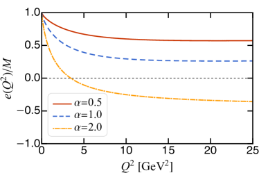
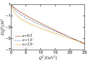
The numerical results of the GFFs are shown in Fig. 13. In this figure, we compare results at various couplings from the perturbative regime to the strong coupling regime , where the dimensionless coupling constant is related to the physical coupling as . In this figure, the term is normalized to unity in the forward limit, viz., , and the term in the same limit is finite and negative . In fact, in our model. Fig. 14 shows the as a function of the coupling . As the coupling increases, becomes more negative. The value of appears quite sensitive to the coupling, thus providing a good probe of the interaction strength of the system. At large , the form factors approach to their one-body contribution, i.e., , and , where is the field strength renormalization constant.
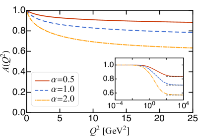
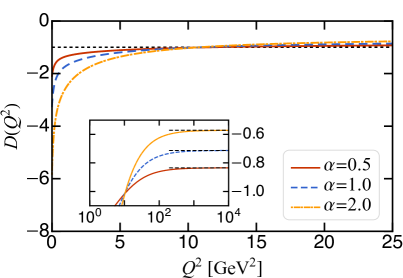
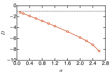
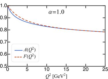
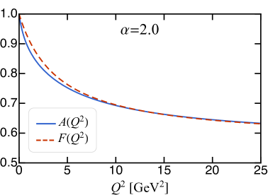
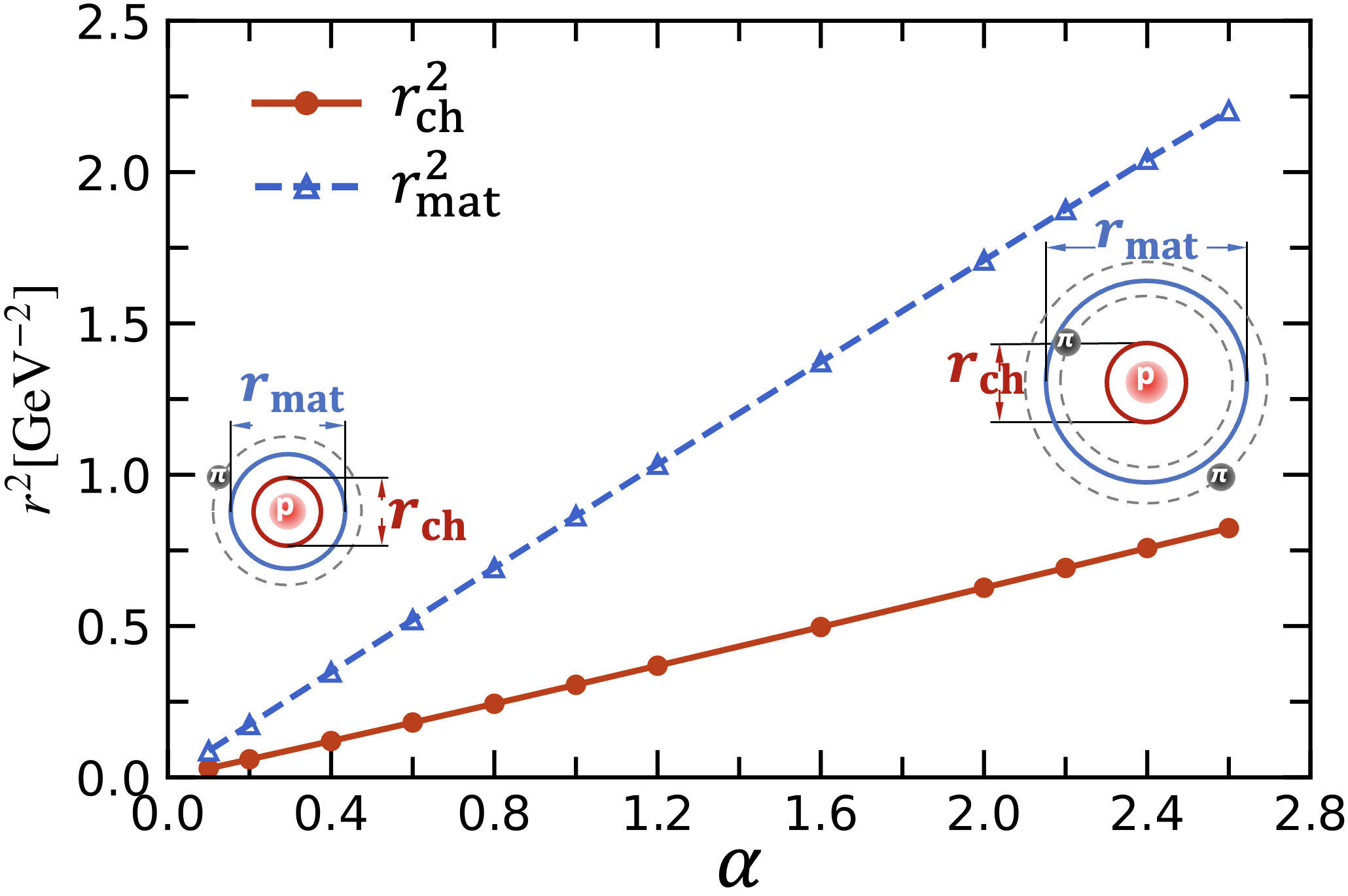
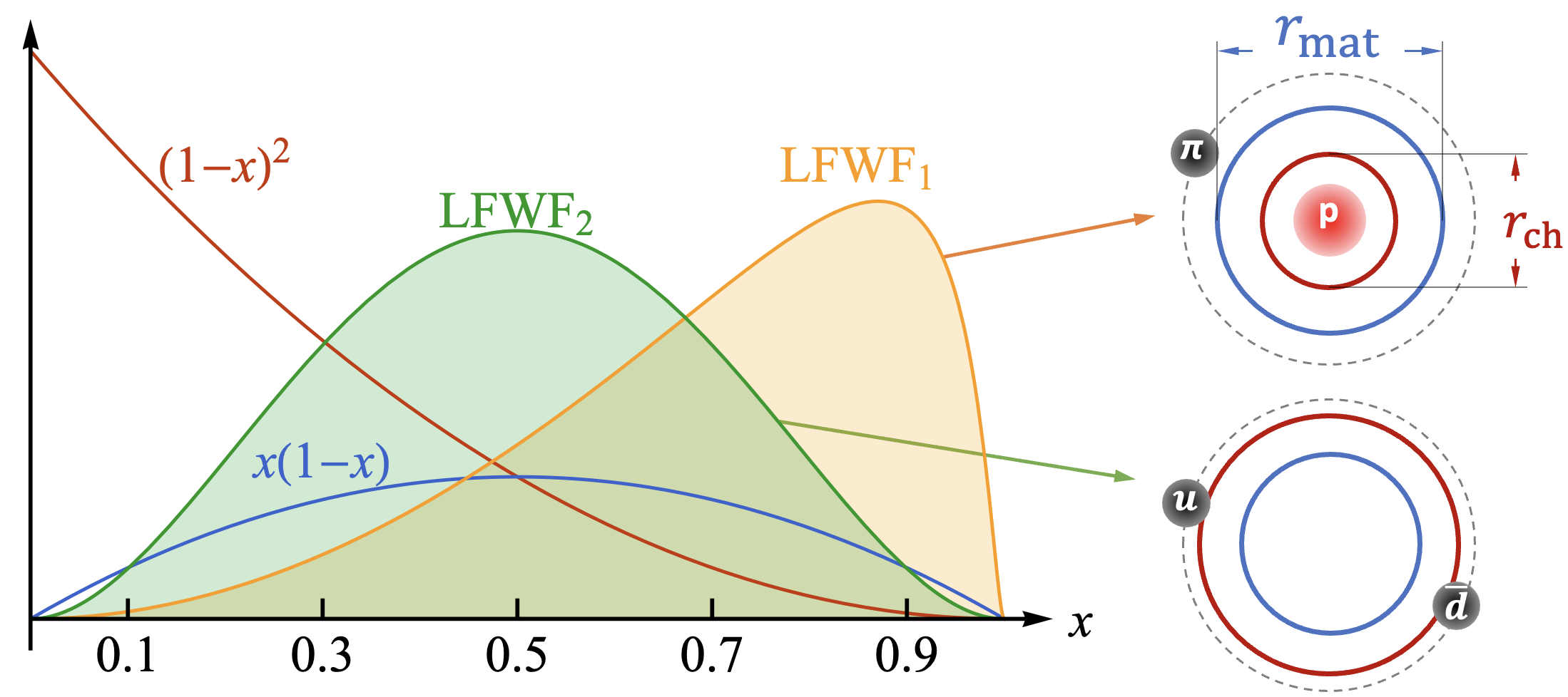
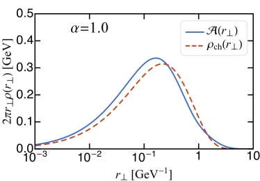
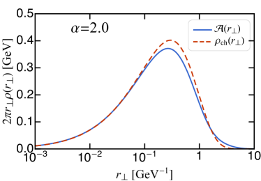
Figure 15 compares the GFF and the charge form factor . Both quantities approach to the same limit at large . However, at small , appears softer than , which implies a larger matter radius than the charge radius, viz., , where and . Indeed, is always larger than for the couplings we consider as shown in Fig. 16. Recall that for mesons, the relative size is reversed Li:2016wwu . These can be understood in the LFWF representation (see Sect. V for more details). In this representation, the charge radius while the matter radius . The cartoon in Fig. 17 illustrates the origins of the mean radii for two systems. For the pion, the LFWF is approximately symmetric with respect to . This shows its charge radius is larger than its matter radius. By contrast, for our pion-dressed proton, the LFWF concentrates on the side, and its matter radius becomes larger than its charge radius.
From the form factors, we can extract the corresponding transverse densities by a Fourier transformation. To avoid the numerical difficulties, we first fit the form factors with the multi-monopole function,
| (101) |
The corresponding density is,
| (102) |
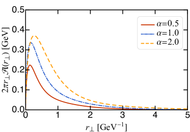
Chiral effective field theory predicts a pion cloud at the periphery of the nucleon transverse charge density () Granados:2013moa ; Granados:2015lxa ; Granados:2015rra . The ansatz we adopt here is qualitatively in agreement with this picture. The extracted matter density444This quantity is also called the mass density, longitudinal momentum density, the tensor density or simply the -density in the literature. However, from our analysis above, is the density associated with all three momenta . On the other hand, both the proper energy density and the invariant mass squared density (Sect. V.2) differ from . For this reason, we feel it is more justified to call this quantity the matter density. is shown in Fig. 18, in comparison with the charge density , the Fourier transform of the charge form factor . Fig. 19 shows the transverse matter density and pressure for various couplings. The expected node within the pressure is squeezed to the origin due to the point-like repulsive core (not shown in the figure).

V Light-front wave function representation
In this section, we further analyze the LFWF representation. Our goal is to obtain a general non-perturbative representation independent of the interactions.
V.1 and the term
We summarize the hadron matrix element computed in Sect. III as follows,
| (103) | ||||
| (104) | ||||
| (105) | ||||
| (106) | ||||
| (107) | ||||
| (108) |
Based on the above expression, it is not hard to conclude a general formula for :
| (109) |
where,
| (110) |
And the -body integration measure is defined as,
| (111) |
where, is the symmetry factor.
Using the transverse coordinate representation introduced in Appendix A, the hadron matrix element (109) can be written as,
| (112) |
The corresponding GFF is,
| (113) |
The light-front distribution is defined as the Fourier transform of the form factor ,
| (114) | ||||
| (115) |
This expression is in agreement with the classic results by Brodsky et al. Brodsky:2000ii . It generalizes the one-body density on the light front. Hence should be understood as the one-body (number) density.
The matter radius is defined as the slope of the form factor multiplied by 6, which is equivalent to times of the mean transverse squared radius,
| (116) |
In LFWF representation,
| (117) |
V.2 and the term
We summarize the hadron matrix element computed in Sect. III as follows. The one-body contribution (diagram , ) is,
| (118) |
The two-body contribution (diagram , , , ) reads,
| (119) | ||||
| (120) | ||||
| (121) |
Similarly, the three-body contribution (diagram , , ) reads,
| (122) | ||||
| (123) | ||||
| (124) |
From the above expressions, the general -body contribution should be,
| (125) |
where,
| (126) | ||||
| (127) | ||||
| (128) |
The first line of Eq. (125) represents the off-forward kinetic energy whereas the second line is the off-forward potential energy (mass eigenvalue minus kinetic energy), thus generalizing Eq. (13) to the off-forward region,
| (129) |
In the transverse coordinate-space,
| (130) |
The corresponding total density is the one-body light-cone energy density
| (131) |
where the one-body (off-forward) kinetic energy density is,
| (132) | ||||
| (133) |
The one-body potential energy density in our case only involves the diagonal Fock sector contributions,
| (134) |
where, is the -body light-cone kinetic energy. Note that the Dirac- only samples the -th parton, the mock nucleon. This is because of the quenched approximation: all interaction is associated with the mock nucleon. It is remarkable that the EMT “knows” the quenched approximation.
The Fourier transforms of , and are the corresponding form factors, , and . At zero-momentum transfer, the squared invariant mass form factor gives the total squared invariant mass . From these expressions, we obtain,
| (135) |
The von Laue mechanical equilibrium condition is automatically fulfilled as long as , a consequence of momentum conservation (97). The GFF is,
| (136) |
In particular, the term is finite,
| (137) |
The term contains a term resembling the virial term. This term measures how the wave function scales in terms of a dilation transformation in the transverse direction. The Fourier transform of the term is a quantity of interest.
| (138) |
The pressure distribution is,
| (139) |
And the proper energy density is,
| (140) |
Note that we have introduced several energy related densities Lorce:2018egm , e.g. , and . is the energy density of the hadron measured in its local rest frame. It is normalized to the hadron rest energy, i.e. hadron mass . is the light-front energy density multiplied by , the state normalization factor. It is normalized to the hadron light-front energy. is the one-body invariant mass squared density. It is the light-front energy density in the Breit frame. It is normalized to the hadron invariant mass squared:
| (141) | ||||
| (142) | ||||
| (143) |
Figure 20 shows the energy form factors, i.e., the Fourier transform of the energy densities.
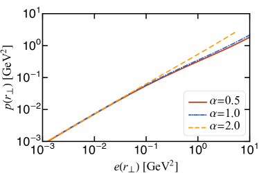
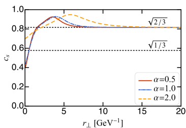
An interesting quantity to investigate is the the pressure as a function of the energy, which can be interpreted as the equation of state Rajan:2018zzy , as shown in Fig. 21. The derivative of the pressure-energy curve, i.e. , is the local speed of the sound. In our model, the speed of the sound exceeds the conformal limit in a large region Altiparmak:2022bke . At the periphery, it approaches .
VI Summary and outlooks
In this work, we computed the forces inside a dressed scalar nucleon in the non-perturbative regime using the light-front Hamiltonian formalism. The calculation is based on a previous non-perturbative solution of the quenched scalar Yukawa model with a systematic Fock sector truncation up to four particles where the Fock sector convergence was demonstrated. The non-perturbative renormalization is implemented using the Fock sector dependent renormalization. In this work, the same counterterms are used to renormalize the hadronic energy-momentum tensor (EMT). The hadron matrix elements of the EMT are computed up to three particles.
Instead of using empirical current components, e.g. , to extract the notoriously challenging term, we performed a detailed analysis of the Lorentz structure of the EMT and concluded that is consistent with the Hamiltonian dynamics that generates the LFWF of the system, and is a reliable current component for extracting the forces inside the composite particles. The extracted term satisfies the von Laue mechanical equilibrium condition. In the forward limit, its value is negative, consistent with the mechanical stability conjecture. term
Using the higher Fock sector expressions, we not only derived the well-known LFWF representation for the term, but also obtained a general LFWF expression for the term. This expression does not involve the details of the interaction, and can be used to investigate the general properties of the forces inside composite particles in the non-perturbative regime. The expression only involves the diagonal Fock sector contributions and thus can be adapted in phenomenological models to investigate the dynamical structures of the nucleons. For example, for effective interactions between the quark and the antiquark, a reasonable approximation is to couple the graviton to the transverse center of mass of the system , i.e.,
| (144) |
where, is the two-body effective interaction. Note that for boost invariant interactions.
An immediate extension of the present work is to incorporate the spin degree of freedom. Another improvement is to lift the quench truncation, which was used to stabilize the scalar theory. Both improvements are required for obtaining a general LFWF representation of the forces in QCD.
The method we used here can also be applied to investigate the inelastic gravitational form factors, which provide a range of applications from particle production near compact stars, to detecting dark matter, and to gravitational transitions Ozdem:2019pkg ; Kim:2022bwn ; Ozdem:2022zig .
Acknowledgements
The authors acknowledge fruitful discussions with S. Xu, C. Mondal, S. Nair, Y. Duan, A. Freese, X. Zhao, K. Serafin and Q. Wang. Y.L. thanks V.A. Karmanov for enlightening discussions on the covariant decomposition of the energy-momentum tensor. Y.L. is supported by the New faculty start-up fund of the University of Science and Technology of China. This work was supported in part by the National Natural Science Foundation of China (NSFC) under Grant No. 12375081, and by the US Department of Energy (DOE) under Grant No. DE-SC0023692.
Appendix A Transverse Coordinate Space Representation
Let us introduce the transverse coordinate space wave function as the Fourier transform of the LFWFs,
| (145) |
where, is the single-particle momentum, and () is the single-particle momentum-space (coordinate-space) light-front wave function. Since the light-front wave functions are boost invariant, the momentum-space wave function can be written in an explicitly boost invariant form,
| (146) |
where, is the relative transverse momentum, and is the total transverse momentum. The -body integration measure can also factorize,
| (147) |
Here, we have denoted,
| (148) |
Taking advantage of the light-front boost invariance, Eq. (145) becomes,
| (149) | ||||
| (150) | ||||
| (151) |
Here, we have introduced the intrinsic coordinate-space wave function,
| (152) |
From Eq. (145), the momentum-space wave function can be expressed as its Fourier transform,
| (153) | ||||
| (154) |
Here, again, and is the total momentum.
Let us next consider the derivatives. From Eqs. (145 & 153), it is not hard to conclude,
| (155) | ||||
| (156) |
Since we work with intrinsic variables, let us reduce the both sides of the second expression,
| (157) | ||||
| (158) | ||||
| (159) | ||||
| (160) | ||||
| (161) |
We can conclude,
| (162) |
Similarly, let us consider
| (163) | ||||
| (164) | ||||
| (165) | ||||
| (166) | ||||
| (167) | ||||
| (168) | ||||
| (169) | ||||
| (170) |
where, . In the last equality, we have used the fact that . We have used a change of variable: . Therefore, we can conclude,
| (171) |
We write the -body integration measure as,
| (172) |
where, is the symmetry factor. The longitudinal measure is,
| (173) |
Recall, the transverse measure is,
| (174) |
We also define a new -body measure based on the transverse coordinates,
| (175) |
References
- (1) M. V. Polyakov and P. Schweitzer, Int. J. Mod. Phys. A 33, no.26, 1830025 (2018) doi:10.1142/S0217751X18300259 [arXiv:1805.06596 [hep-ph]].
- (2) V. D. Burkert, L. Elouadrhiri, F. X. Girod, C. Lorcé, P. Schweitzer and P. E. Shanahan, [arXiv:2303.08347 [hep-ph]].
- (3) I. Y. Kobzarev and L. B. Okun, Zh. Eksp. Teor. Fiz. 43, 1904-1909 (1962); [Sov. Phys. JETP 16 (1963) 1343-1346]
- (4) H. Pagels, Phys. Rev. 144, 1250-1260 (1966) doi:10.1103/PhysRev.144.1250
- (5) I. A. Perevalova, M. V. Polyakov and P. Schweitzer, Phys. Rev. D 94, no.5, 054024 (2016) doi:10.1103/PhysRevD.94.054024 [arXiv:1607.07008 [hep-ph]].
- (6) X. D. Ji, W. Melnitchouk and X. Song, Phys. Rev. D 56, 5511-5523 (1997) doi:10.1103/PhysRevD.56.5511 [arXiv:hep-ph/9702379 [hep-ph]].
- (7) V. Y. Petrov, P. V. Pobylitsa, M. V. Polyakov, I. Bornig, K. Goeke and C. Weiss, Phys. Rev. D 57, 4325-4333 (1998) doi:10.1103/PhysRevD.57.4325 [arXiv:hep-ph/9710270 [hep-ph]].
- (8) M. V. Polyakov, Nucl. Phys. B 555, 231 (1999) doi:10.1016/S0550-3213(99)00314-4 [arXiv:hep-ph/9809483 [hep-ph]].
- (9) M. V. Polyakov, Phys. Lett. B 555, 57-62 (2003) doi:10.1016/S0370-2693(03)00036-4 [arXiv:hep-ph/0210165 [hep-ph]].
- (10) V. Guzey and M. Siddikov, J. Phys. G 32, 251-268 (2006) doi:10.1088/0954-3899/32/3/002 [arXiv:hep-ph/0509158 [hep-ph]].
- (11) C. Cebulla, K. Goeke, J. Ossmann and P. Schweitzer, Nucl. Phys. A 794, 87-114 (2007) doi:10.1016/j.nuclphysa.2007.08.004 [arXiv:hep-ph/0703025 [hep-ph]].
- (12) B. Pasquini and S. Boffi, Phys. Lett. B 653, 23-28 (2007) doi:10.1016/j.physletb.2007.07.037 [arXiv:0705.4345 [hep-ph]].
- (13) D. S. Hwang and D. Mueller, Phys. Lett. B 660, 350-359 (2008) doi:10.1016/j.physletb.2008.01.014 [arXiv:0710.1567 [hep-ph]].
- (14) M. Mai and P. Schweitzer, Phys. Rev. D 86, 076001 (2012) doi:10.1103/PhysRevD.86.076001 [arXiv:1206.2632 [hep-ph]].
- (15) M. Mai and P. Schweitzer, Phys. Rev. D 86, 096002 (2012) doi:10.1103/PhysRevD.86.096002 [arXiv:1206.2930 [hep-ph]].
- (16) J. H. Jung, U. Yakhshiev and H. C. Kim, J. Phys. G 41, 055107 (2014) doi:10.1088/0954-3899/41/5/055107 [arXiv:1310.8064 [hep-ph]].
- (17) M. Cantara, M. Mai and P. Schweitzer, Nucl. Phys. A 953, 1-20 (2016) doi:10.1016/j.nuclphysa.2016.04.032 [arXiv:1510.08015 [hep-ph]].
- (18) J. Hudson and P. Schweitzer, Phys. Rev. D 97, no.5, 056003 (2018) doi:10.1103/PhysRevD.97.056003 [arXiv:1712.05317 [hep-ph]].
- (19) M. V. Polyakov and H. D. Son, JHEP 09, 156 (2018) doi:10.1007/JHEP09(2018)156 [arXiv:1808.00155 [hep-ph]].
- (20) D. Chakrabarti, C. Mondal, A. Mukherjee, S. Nair and X. Zhao, Phys. Rev. D 102, 113011 (2020) doi:10.1103/PhysRevD.102.113011 [arXiv:2010.04215 [hep-ph]].
- (21) A. Metz, B. Pasquini and S. Rodini, Phys. Lett. B 820, 136501 (2021) doi:10.1016/j.physletb.2021.136501 [arXiv:2104.04207 [hep-ph]].
- (22) K. A. Mamo and I. Zahed, Phys. Rev. D 106, no.8, 086004 (2022) doi:10.1103/PhysRevD.106.086004 [arXiv:2204.08857 [hep-ph]].
- (23) M. Fujita, Y. Hatta, S. Sugimoto and T. Ueda, PTEP 2022, no.9, 093B06 (2022) doi:10.1093/ptep/ptac110 [arXiv:2206.06578 [hep-th]].
- (24) J. More, A. Mukherjee, S. Nair and S. Saha, Phys. Rev. D 105, no.5, 056017 (2022) doi:10.1103/PhysRevD.105.056017 [arXiv:2112.06550 [hep-ph]].
- (25) A. Garcia Martin-Caro, Y. Hatta and M. Huidobro, [arXiv:2304.05994 [nucl-th]].
- (26) A. Amor-Quiroz, W. Focillon, C. Lorcé and S. Rodini, [arXiv:2304.10339 [hep-ph]].
- (27) J. More, A. Mukherjee, S. Nair and S. Saha, Phys. Rev. D 107, no.11, 116005 (2023) doi:10.1103/PhysRevD.107.116005 [arXiv:2302.11906 [hep-ph]].
- (28) A. Freese, A. Metz, B. Pasquini and S. Rodini, Phys. Lett. B 839, 137768 (2023) doi:10.1016/j.physletb.2023.137768 [arXiv:2212.12197 [hep-ph]].
- (29) D. Chakrabarti, P. Choudhary, B. Gurjar, R. Kishore, T. Maji, C. Mondal and A. Mukherjee, Phys. Rev. D 108, no.1, 014009 (2023) doi:10.1103/PhysRevD.108.014009 [arXiv:2304.09908 [hep-ph]].
- (30) X. Ji and Y. Liu, Phys. Rev. D 106, no.3, 034028 (2022) doi:10.1103/PhysRevD.106.034028 [arXiv:2110.14781 [hep-ph]].
- (31) X. D. Ji, Phys. Rev. Lett. 74, 1071-1074 (1995) doi:10.1103/PhysRevLett.74.1071 [arXiv:hep-ph/9410274 [hep-ph]].
- (32) C. Lorcé, H. Moutarde and A. P. Trawiński, Eur. Phys. J. C 79, no.1, 89 (2019) doi:10.1140/epjc/s10052-019-6572-3 [arXiv:1810.09837 [hep-ph]].
- (33) C. Lorcé, A. Metz, B. Pasquini and S. Rodini, JHEP 11, 121 (2021) doi:10.1007/JHEP11(2021)121 [arXiv:2109.11785 [hep-ph]].
- (34) O. Teryaev, Nucl. Phys. B Proc. Suppl. 245, 195-198 (2013) doi:10.1016/j.nuclphysbps.2013.10.039 [arXiv:1309.1985 [hep-ph]].
- (35) X. D. Ji, Phys. Rev. D 55, 7114-7125 (1997) doi:10.1103/PhysRevD.55.7114 [arXiv:hep-ph/9609381 [hep-ph]].
- (36) V. D. Burkert, L. Elouadrhiri and F. X. Girod, Nature 557, no.7705, 396-399 (2018) doi:10.1038/s41586-018-0060-z
- (37) V. D. Burkert, L. Elouadrhiri and F. X. Girod, [arXiv:2104.02031 [nucl-ex]].
- (38) K. Kumerički, Nature 570, no.7759, E1-E2 (2019) doi:10.1038/s41586-019-1211-6
- (39) H. Dutrieux, C. Lorcé, H. Moutarde, P. Sznajder, A. Trawiński and J. Wagner, Eur. Phys. J. C 81, no.4, 300 (2021) doi:10.1140/epjc/s10052-021-09069-w [arXiv:2101.03855 [hep-ph]].
- (40) A. Accardi, J. L. Albacete, M. Anselmino, N. Armesto, E. C. Aschenauer, A. Bacchetta, D. Boer, W. K. Brooks, T. Burton and N. B. Chang, et al. Eur. Phys. J. A 52, no.9, 268 (2016) doi:10.1140/epja/i2016-16268-9 [arXiv:1212.1701 [nucl-ex]].
- (41) D. P. Anderle, V. Bertone, X. Cao, L. Chang, N. Chang, G. Chen, X. Chen, Z. Chen, Z. Cui and L. Dai, et al. Front. Phys. (Beijing) 16, no.6, 64701 (2021) doi:10.1007/s11467-021-1062-0 [arXiv:2102.09222 [nucl-ex]].
- (42) A. Accardi, P. Achenbach, D. Adhikari, A. Afanasev, C. S. Akondi, N. Akopov, M. Albaladejo, H. Albataineh, M. Albrecht and B. Almeida-Zamora, et al. [arXiv:2306.09360 [nucl-ex]].
- (43) S. Kumano, Q. T. Song and O. V. Teryaev, Phys. Rev. D 97, no.1, 014020 (2018) doi:10.1103/PhysRevD.97.014020 [arXiv:1711.08088 [hep-ph]].
- (44) D. E. Kharzeev, Phys. Rev. D 104, no.5, 054015 (2021) doi:10.1103/PhysRevD.104.054015 [arXiv:2102.00110 [hep-ph]].
- (45) P. E. Shanahan and W. Detmold, Phys. Rev. Lett. 122, no.7, 072003 (2019) doi:10.1103/PhysRevLett.122.072003 [arXiv:1810.07589 [nucl-th]].
- (46) D. C. Hackett, P. R. Oare, D. A. Pefkou and P. E. Shanahan, [arXiv:2307.11707 [hep-lat]].
- (47) I. V. Anikin, Phys. Rev. D 99, no.9, 094026 (2019) doi:10.1103/PhysRevD.99.094026 [arXiv:1902.00094 [hep-ph]].
- (48) X. B. Tong, J. P. Ma and F. Yuan, JHEP 10, 046 (2022) doi:10.1007/JHEP10(2022)046 [arXiv:2203.13493 [hep-ph]].
- (49) Z. Xing, M. Ding and L. Chang, Phys. Rev. D 107, no.3, L031502 (2023) doi:10.1103/PhysRevD.107.L031502 [arXiv:2211.06635 [hep-ph]].
- (50) S. J. Brodsky, H. C. Pauli and S. S. Pinsky, Phys. Rept. 301, 299-486 (1998) doi:10.1016/S0370-1573(97)00089-6 [arXiv:hep-ph/9705477 [hep-ph]].
- (51) B. L. G. Bakker, A. Bassetto, S. J. Brodsky, W. Broniowski, S. Dalley, T. Frederico, S. D. Glazek, J. R. Hiller, C. R. Ji and V. Karmanov, et al. Nucl. Phys. B Proc. Suppl. 251-252, 165-174 (2014) doi:10.1016/j.nuclphysbps.2014.05.004 [arXiv:1309.6333 [hep-ph]].
- (52) F. Gross, E. Klempt, S. J. Brodsky, A. J. Buras, V. D. Burkert, G. Heinrich, K. Jakobs, C. A. Meyer, K. Orginos and M. Strickland, et al. [arXiv:2212.11107 [hep-ph]].
- (53) R. P. Feynman, Phys. Rev. Lett. 23, 1415-1417 (1969) doi:10.1103/PhysRevLett.23.1415
- (54) J. B. Kogut and L. Susskind, Phys. Rept. 8, 75-172 (1973) doi:10.1016/0370-1573(73)90009-4
- (55) S. J. Brodsky and G. P. Lepage, Phys. Rev. D 24, 1808 (1981) doi:10.1103/PhysRevD.24.1808
- (56) G. A. Miller, Ann. Rev. Nucl. Part. Sci. 60, 1-25 (2010) doi:10.1146/annurev.nucl.012809.104508 [arXiv:1002.0355 [nucl-th]].
- (57) X. Ji and Y. Liu, Phys. Rev. D 105, no.7, 076014 (2022) doi:10.1103/PhysRevD.105.076014 [arXiv:2106.05310 [hep-ph]].
- (58) Y. Li, “Ab initio approach to quantum field theories on the light front,” Ph.D. thesis. https://doi.org/10.31274/etd-180810-4540
- (59) S. Xu, C. Mondal, X. Zhao, Y. Li and J. P. Vary, [arXiv:2209.08584 [hep-ph]].
- (60) M. Kreshchuk, S. Jia, W. M. Kirby, G. Goldstein, J. P. Vary and P. J. Love, Phys. Rev. A 103, no.6, 062601 (2021) doi:10.1103/PhysRevA.103.062601 [arXiv:2011.13443 [quant-ph]].
- (61) W. Qian, R. Basili, S. Pal, G. Luecke and J. P. Vary, Phys. Rev. Res. 4, no.4, 043193 (2022) doi:10.1103/PhysRevResearch.4.043193 [arXiv:2112.01927 [quant-ph]].
- (62) J. P. Vary, L. Adhikari, G. Chen, M. Li, Y. Li, P. Maris, W. Qian, J. R. Spence, S. Tang and K. Tuchin, et al. Few Body Syst. 58, no.2, 56 (2017) doi:10.1007/s00601-016-1210-1 [arXiv:1612.03963 [nucl-th]].
- (63) S. J. Brodsky, D. S. Hwang, B. Q. Ma and I. Schmidt, Nucl. Phys. B 593, 311-335 (2001) doi:10.1016/S0550-3213(00)00626-X [arXiv:hep-th/0003082 [hep-th]].
- (64) M. J. Godfrey, Phys. Rev. B 37, 10176 (1988)
- (65) C. L. Rogers and A. M. Rappe. Phys. Rev. B 65 (2001): 224117.
- (66) J. Lan et al. [BLFQ], Phys. Lett. B 825, 136890 (2022) doi:10.1016/j.physletb.2022.136890 [arXiv:2106.04954 [hep-ph]].
- (67) B. Pasquini et al. [MAP (Multi-dimensional Analyses of Partonic distributions)], Phys. Rev. D 107, no.11, 114023 (2023) doi:10.1103/PhysRevD.107.114023 [arXiv:2303.01789 [hep-ph]].
- (68) P. V. Pobylitsa, Phys. Rev. D 67, 094012 (2003) doi:10.1103/PhysRevD.67.094012 [arXiv:hep-ph/0210238 [hep-ph]].
- (69) M. V. Polyakov and C. Weiss, Phys. Rev. D 60, 114017 (1999) doi:10.1103/PhysRevD.60.114017 [arXiv:hep-ph/9902451 [hep-ph]].
- (70) V. A. Karmanov, J. F. Mathiot and A. V. Smirnov, Phys. Rev. D 77, 085028 (2008) doi:10.1103/PhysRevD.77.085028 [arXiv:0801.4507 [hep-th]].
- (71) V. A. Karmanov, Y. Li, A. V. Smirnov and J. P. Vary, Phys. Rev. D 94, no.9, 096008 (2016) doi:10.1103/PhysRevD.94.096008 [arXiv:1610.03559 [hep-th]].
- (72) Y. Li, V. A. Karmanov, P. Maris and J. P. Vary, Phys. Lett. B 748, 278-283 (2015) doi:10.1016/j.physletb.2015.07.014 [arXiv:1504.05233 [nucl-th]].
- (73) J. Carbonell, B. Desplanques, V. A. Karmanov and J. F. Mathiot, Phys. Rept. 300, 215-347 (1998) doi:10.1016/S0370-1573(97)00090-2 [arXiv:nucl-th/9804029 [nucl-th]].
- (74) F. Gross, C. Savkli and J. Tjon, Phys. Rev. D 64, 076008 (2001) doi:10.1103/PhysRevD.64.076008 [arXiv:nucl-th/0102041 [nucl-th]].
- (75) P. A. M. Dirac, Rev. Mod. Phys. 21, 392-399 (1949) doi:10.1103/RevModPhys.21.392
- (76) S. Weinberg, Phys. Rev. 150, 1313-1318 (1966) doi:10.1103/PhysRev.150.1313
- (77) V. A. Karmanov, Zh. Eksp. Teor. Fiz. 71, 399-416 (1976); [Sov. Phys. JETP 44, 210 (1976)]
- (78) S. D. Drell and T. M. Yan, Phys. Rev. Lett. 24, 181-185 (1970) doi:10.1103/PhysRevLett.24.181
- (79) Yang Li, X.h. Cao, Q. Wang, and J. P. Vary, Hadronic energy-momentum tensor revisited, in preparation.
- (80) M. Varma and P. Schweitzer, Phys. Rev. D 102, no.1, 014047 (2020) doi:10.1103/PhysRevD.102.014047 [arXiv:2006.06602 [hep-ph]].
- (81) M. Laue, Annalen Phys. 340, no.8, 524-542 (1911) doi:10.1002/andp.19113400808
- (82) Y. Li, Few Body Syst. 58, no.3, 109 (2017) doi:10.1007/s00601-017-1266-6 [arXiv:1612.01259 [nucl-th]].
- (83) C. Granados and C. Weiss, JHEP 01, 092 (2014) doi:10.1007/JHEP01(2014)092 [arXiv:1308.1634 [hep-ph]].
- (84) C. Granados and C. Weiss, Phys. Rev. C 92, no.2, 025206 (2015) doi:10.1103/PhysRevC.92.025206 [arXiv:1503.02055 [hep-ph]].
- (85) C. Granados and C. Weiss, JHEP 07, 170 (2015) doi:10.1007/JHEP07(2015)170 [arXiv:1503.04839 [hep-ph]].
- (86) A. Rajan, T. Gorda, S. Liuti and K. Yagi, [arXiv:1812.01479 [hep-ph]].
- (87) S. Altiparmak, C. Ecker and L. Rezzolla, Astrophys. J. Lett. 939, no.2, L34 (2022) doi:10.3847/2041-8213/ac9b2a [arXiv:2203.14974 [astro-ph.HE]].
- (88) U. Özdem and K. Azizi, Phys. Rev. D 101, no.5, 054031 (2020) doi:10.1103/PhysRevD.101.054031 [arXiv:1912.06375 [hep-ph]].
- (89) J. Y. Kim, Phys. Lett. B 834, 137442 (2022) doi:10.1016/j.physletb.2022.137442 [arXiv:2206.10202 [hep-ph]].
- (90) U. Özdem and K. Azizi, JHEP 03, 048 (2023) doi:10.1007/JHEP03(2023)048 [arXiv:2212.07290 [hep-ph]].