Homological algebra and moduli spaces in topological field theories

1. Numerical invariants: Donaldson and Gromov.

The relations between topology and linear partial differential equations are classical going back to 19 century and a recent high point is Atiyah-Singer index theorem. The relations between non-linear differential equations and geometry are very hot and active topics which become big trends after several important discoveries in the 1970’s. More recently relations between moduli spaces of the solutions of non-linear differential equations and ‘topology’ are discovered and become an important topic.

In his famous paper [D1], Donaldson used the moduli space of the solutions of Yang-Mills equation to obtain novel restrictions on the intersection forms of closed 4-dimensional manifolds. In subsequent papers [D2, D3], the moduli space is used to obtain an invariant of a closed smooth 4-dimensional manifold.

Let $X$ be a closed $4$-dimensional manifold and $\mathcal{E}_{X}\to X$ an $SU(2)$ bundle. A connection $A$ of $\mathcal{E}_{X}$ is said to be an ASD (anti-self-dual) connection, if it satisfies the equation:

$$F_{A}+*_{X}F_{A}=0.$$ (1.1)

Here $F_{A}$ is the curvature of $A$ and $*_{X}$ is the Hodge $*$ operator. Note that $*_{X}$ depends on the choice of a Riemannian metric on $X$. The set of solutions of (1.1) is invariant under the action of the gauge transformation group (the set of automorphisms of the principal bundle $\mathcal{E}_{X}\to X$). We denote by $\mathcal{M}(X;\mathcal{E}_{X})$ the set of gauge equivalence classes of the solutions of (1.1). The space $\mathcal{M}(X;\mathcal{E}_{X})$ has the following nice properties.

1. The moduli space $\mathcal{M}(X;\mathcal{E}_{X})$ is generically a smooth manifold outside the set of points corresponding to the reducible connections.

2. The space $\mathcal{M}(X;\mathcal{E}_{X})$ has a nice compactification called the Uhlenbeck compactification.

3. The ‘cobordism class’ of $\mathcal{M}(X;\mathcal{E}_{X})$ is independent of various choices.

In the case of $SU(2)$ bundles, a reducible connection is induced from a $U(1)$ connection. The curvature of an anti-self-dual $U(1)$ connection is a harmonic two form $h$ with $*_{X}h=-h$. So the negative eigen-space on the second cohomology group $H^{2}(X;{\mathbb{R}})$ (with respect to the intersection form) is related to the singularity of $\mathcal{M}(X;\mathcal{E}_{X})$. We denote by $b_{2}^{+}$ and $b_{2}^{-}$ the dimensions of positive and negative eigen-spaces on the second cohomology group $H^{2}(X;{\mathbb{R}})$ with respect to the intersection form. If $b_{2}^{+}=0$ (and $b_{2}^{-}\neq 0$) then for any Riemannian metric on $X$ there exists a harmonic 2 form $h$ representing integral cohomology classes and satisfying $*_{X}h=-h$. It implies that there exists a reducible connection for any Riemannian metric. In general, the set of Riemannian metrics for which $\mathcal{M}(X;\mathcal{E}_{X})$ contains a reducible connection has codimension $b_{2}^{+}$. Thus $\mathcal{M}(X;\mathcal{E}_{X})$ is ‘closer’ to a non-singular space (manifold) if $b_{2}^{+}$ is large. In fact the Donaldson invariant is well-defined if $b_{2}^{+}\geq 2$ but is not defined if $b_{2}^{+}=0$. The case $b_{2}^{+}=1$ is a borderline case where the invariant exists but depends on the ‘chamber’ in which the Riemannian metric is contained. Namely it depends on the metric however we can control the way how it changes when a family of Riemannian metrics crosses the ‘wall’ and moves from one chamber to the other. The case $b_{2}^{+}=1$ is used in [D2] to obtain the first example of a pair of closed $4$-dimensional manifolds which are homeomorphic but are not diffeomorphic.

In the simplest case, that is, when the (virtual) dimension $\mathcal{M}(X;\mathcal{E}_{X})$ is zero, Donaldson invariant is a number. In general Donaldson introduced and used a certain cohomology class to cut down the space $\mathcal{M}(X;\mathcal{E}_{X})$ and obtain a number. He used a map

$$\nu:H_{*}(X;{\mathbb{Z}})\to H^{4-*}(\mathcal{B}^{*}(X;\mathcal{E}_{X});{\mathbb{Z}}).$$

Here $\mathcal{B}^{*}(X;\mathcal{E}_{X})$ is the set of gauge equivalence classes of the irreducible connections of $\mathcal{E}_{X}$. Donaldson invariant can be regarded as a polynomial on $H_{*}(X;{\mathbb{Z}})$ and written as

$$Q(a_{1},\dots,a_{k})=\int_{\mathcal{M}(X;\mathcal{E}_{X})}\nu(a_{1})\wedge\dots\nu(a_{k}).$$ (1.2)

(ASD3) ‘implies’ that this number is independent of the Riemannian metric etc. and becomes an invariant of a smooth 4-dimensional manifold.

A certain delicate (dimension counting type) argument is necessary to understand how the reducible connections and the infinity of the Uhlenbeck compactification affect the well-defined-ness of the integral (1.2).

Gromov [Gr] introduced the method of pseudo-holomorphic curve to symplectic geometry. For a symplectic manifold $(X,\omega)$ Gromov considered a compatible almost complex structure $J$, that is, a tensor $J:TX\to TX$ such that $J^{2}=-1$ and $g(V,W):=\omega(V,JW)$ becomes a Riemannian metric. Then a pseudo-holomorphic curve is a map $u$ from a Rieman surface $(\Sigma,j_{\Sigma})$ to $(X,J)$ such that

$$J\circ Du=Du\circ j_{\Sigma}.$$ (1.3)

The equation (1.3) is also written as

$$\overline{\partial}u=0.$$ (1.4)

Here it is very important that $J$ is an almost complex structure which is not necessary integrable. If $J$ is an integrable complex structure we can take a complex coordinate of $X$ so that $J=\sqrt{-1}$ is constant. Then writing $u=(u^{1},\dots,u^{n})$ by the complex coordinate, (1.3) becomes

$$\frac{\partial u^{i}}{\partial y}=\sqrt{-1}\frac{\partial u^{i}}{\partial x},$$ (1.5)

where $z=x+\sqrt{-1}y$ is a complex coordinate of the Rieman surface $(\Sigma,j_{\Sigma})$. The equation (1.5) is a linear partial differential equation. On the other hand, (1.3) is non-linear. An important observation by Gromov is that the non-linear partial differential equation (1.3) can have lots of solutions in the case when the domain has complex dimension one. In fact if $(Y,j)$ is a complex two dimensional manifold, typically there is no non-constant map $u:Y\to X$ satisfying $J\circ Du=Du\circ j$ in the case when $J$ is not integrable.

Another important point is in the case when the almost complex structure $J$ is compatible with a certain symplectic structure the moduli space of solutions of the equation (1.3) has a nice compactification. In fact we have the following properties. We fix a non-negative integer $g$ and a positive number $E$ and for a symplectic manifold $X$ with compatible almost complex structure $J$, we denote by $\overset{\circ}{\mathcal{M}}_{g}(X,J;E)$ the set of pairs $((\Sigma,j),u)$ where $(\Sigma,j)$ is a Rieman surface of genus $g$ and $u:\Sigma\to X$ satisfies the equation (1.3). We also require

$$\int_{\Sigma}u^{*}\omega\leq E.$$

1. The moduli space $\overset{\circ}{\mathcal{M}}_{g}(X,J;E)$ is generically a smooth manifold.

2. The space $\overset{\circ}{\mathcal{M}}_{g}(X,J;E)$ has a nice compactification.

3. The ‘cobordism class’ of the compactification ${\mathcal{M}}_{g}(X,J;E)$ is independent of the various choices especially of the choice of the almost complex structure.

These properties are similar to the properties (ASD1), (ASD2), (ASD3). Gromov used them to prove that, for any almost complex structure $J$ on ${\mathbb{C}}P^{2}$ which is compatible with the standard symplectic structure, there exists a pseudo-holomorphic curve $u:S^{2}\to({\mathbb{C}}P^{2},J)$ whose homology class is the generator of $H_{2}({\mathbb{C}}P^{2})$. This fact has an important application which is called non-sqeezing theorem.

Theorem 1.1.

([Gr]) If there exists a map $u$ from $\overset{\circ}{D^{4}}(r)$ (the open $r$-ball in ${\mathbb{C}}^{2}$) to $D^{2}(1)\times{\mathbb{C}}$ such that $u^{*}\omega=\omega$ (where $\omega$ is the standard symplectic form) then $r<1$.

It implies, for example, that $\overset{\circ}{D^{4}}(1)$ is not symplectomorphic to $\overset{\circ}{D^{2}}(2)\times\overset{\circ}{D^{2}}(1/2)$. This is one of the first results which show the ‘existence of global symplectic geometry’.

Around the same time, physicists working on string theory studied ‘topological’ version of string theory and the ‘invariant’ obtained by integrating a certain cohomology class on the moduli space which can be regarded as a compactification of $\overset{\circ}{\mathcal{M}}_{g}(X,J;E)$. (See for example [Wi3].) One point which is not so clear from physicists’ point of view is the fact that such ‘invariant’ is one of symplectic structure and not one of almost complex structure (or complex structure). On the other hand, various important properties of the invariant (obtained from the moduli space of pseudo-holomorphic curves) are discovered by physicists. Among them the associativity of the product structure obtained from a pseudo-holomorphic map $S^{2}\to X$ is very important (see [Va]).

Ruan [Ru1] and Ruan-Tian [RT1, RT2] established the theory of invariants obtained from the moduli space of pseudo-holomorphic curves. After McDuff-Salamon’s lucid exposition [McSa] appeared this theory becomes popular among differential and symplectic geometers.

2. Floer homology.

Floer homology was discovered in the 1980’s (by A. Floer) in two areas. One is gauge theory and the other is symplectic geometry. Floer’s work is a development of three important works in those areas.

1. Casson invariant of 3-dimensional manifolds (See [AM]) and Taubes’ work [Ta] to relate it to gauge theory.

2. Conley-Zehnder’s proof [CZ] of Arnold’s conjecture for tori. (There was a related work [Ra] before that.)

3. Witten’s work [Wi1] which relates Morse theory to a (supersymmetric) quantum field theory.

All of these are famous and important works. We mention them briefly.

For a 3-dimensional manifold $M^{3}$, which is a homology 3-sphere, Casson defined an integer valued invartiant, the Casson invariant, which is morally the ‘number’ of flat $SU(2)$-connections on $M^{3}$. The ‘virtual’ dimension of the moduli space of flat $SU(2)$-connections on $M^{3}$ is $0$. However because of failure of transversality the number of flat connections in the naive sense may be infinite. Also, as in the case of intersection theory in differential geometry or topology, the ‘number’ should be counted with sign. Casson’s way to count the number of flat $SU(2)$-connections on $M$ uses Heegaard splitting of $M$ into the union of two handle bodies $M=H^{1}_{g}\cup_{\Sigma_{g}}H^{2}_{g}$. Here $\Sigma_{g}$ is an oriented 2-dimensional manifold of genus $g$ and $H_{g}\cong H_{g}^{1}\cong H_{g}^{2}$ are the handle bodies which bound $\Sigma_{g}$. The moduli space $R(\Sigma_{g})$ of flat $SU(2)$-connections on the trivial bundle on $\Sigma_{g}$ is a singular space of dimension $6g-6$. The moduli spaces $R(H_{g}^{i})$ of flat $SU(2)$-connections on the trivial bundle on the handle bodies $H_{g}^{i}$ become subspaces of $R(\Sigma)$ of dimension $3g-3$. Casson defined Casson invariant $Z(M)$ as the ‘intersection number’

$$Z(M):=R(H_{g}^{1})\cdot R(H_{g}^{2})\in\mathbb{Z}$$

of two $3g-3$ dimensional subspaces in the $6g-g$ dimensional space $R(\Sigma_{g})$. The points to be worked out are the following:

1. The intersection number is well-defined even though $R(\Sigma_{g})$ and $R(H_{g}^{i})$ have singularities.

2. The number $Z(M)$ is independent of the choices of Heegaard splitting $M\cong H_{g}^{1}\cup_{\Sigma_{g}}H_{g}^{2}$ and $g$. It becomes an invariant of the 3-dimensional manifold $M$.

Casson proved them in the case when $H(M;\mathbb{Z})=H(S^{3};\mathbb{Z})$. Note that this assumption implies that the intersection points $R(H_{g}^{1})\cap R(H_{g}^{2})$ are not singular points of $R(\Sigma_{g})$ unless it is the point corresponding to the trivial connection.

Taubes’ work [Ta] gave an alternative construction. In place of using Heegaard splitting Taubes studied the set of all connections $\mathcal{B}(M;SU(2))$ (modulo the gauge transformation group) and regard the condition $F_{A}=0$ (the curvature is $0$) as a differential equation. In the case when the set of flat connections on $M$ is not transversal this equation is not transversal. Taubes then perturbed the equation $F_{A}=0$ so that after adding an appropriate perturbation term $\mu(A)$ the set of solutions of the equation $F_{A}+\mu(A)=0$ becomes isolated. He then counted its order. This construction works under the assumption $H(M;\mathbb{Z})=H(S^{3};\mathbb{Z})$ since otherwise there are reducible connections other than the trivial one, which causes trouble. Taubes then proved that the invariant by such a count is equal to one obtained by Heegaard splitting.

Defining an invariant of 3-dimensional manifolds is one of the applications of Floer homology. The other application is to symplectic geometry especially to Arnold’s conjecture on the periodic orbits of a periodic Hamiltonian system. Conley-Zehnder [CZ] proved it in the case of (symplectic) torus $T^{2n}$, as follows. Let $H:T^{2n}\times S^{1}\to{\mathbb{R}}$ be a smooth function. For $t\in S^{1}$, we put $H_{t}(x)=H(x,t)$ and let $\mathfrak{X}_{H_{t}}$ be the Hamiltonian vector field associated to the function $H_{t}$ with respect to a certain symplectic structure $T^{2n}$ (with constant coefficient). We consider the set $\mathcal{PER}_{H}$ of solutions of the equation

$$\frac{d}{dt}\gamma=\mathfrak{X}_{H_{t}}\circ\gamma$$ (2.1)

where $\gamma:S^{1}\to T^{2n}$. Conley-Zehnder proved that the order of $\mathcal{PER}_{H}$ is not smaller than $2^{2n}$, the Betti-number of $T^{2n}$, under a certain non-degeneracy condition. A solution of Equation (2.1) can be regarded as a critical point of the action functional $\mathcal{A}_{H}$ defined by

$$\mathcal{A}_{H}(\gamma)=-\int_{D^{2}}u^{*}\omega+\int_{S^{1}}H(\gamma(t),t)dt.$$ (2.2)

Here we consider only the loops $\gamma:S^{1}\to T^{2n}$ which are homotopic to the constant map and $u:D^{2}\to T^{2n}$ is a map such that $u|_{\partial D^{2}}=\gamma$. The integral of the symplectic form $\omega$ which is the first term of the right hand side is independent of the choice of $u$, because of Stokes’ theorem, since $\pi_{2}(T^{2n})=0$. The fact that a periodic solution of Hamilton equation (2.1) is a critical point of the action functional $\mathcal{A}_{H}$ is a classical fact (maybe discovered by Hamilton himself). However it had been difficult to use ‘Morse theory’ of action functional $\mathcal{A}_{H}$ to study periodic solutions of Hamilton equation (2.1). In fact the properties of $\mathcal{A}_{H}$ are far from many of the functionals studied in geometric analysis. In the case when the functional $\mathfrak{F}$ satisfies a condition that $\{x\mid\mathfrak{F}(x)\leq c\}$ is ‘compact’ in a certain weak sense (Palais-Smale’s condition C is a typical way to formulate it), then one can show that the set of critical points of $\mathfrak{F}$ is related to the topology of the configuration space. However in the case of the action functional $\mathcal{A}_{H}$ such ‘compactness’ does not hold in any reasonable sense. In fact the set of critical points of $\mathcal{A}_{H}$ is related to the topology of $T^{2n}$ but not to the topology of the loop space $\Omega(T^{2n})$.

Conley-Zehnder [CZ] used a finite dimensional approximation of the loop space $\Omega(T^{2n})$ by Fourier expansion and used an appropriate finite dimensional approximation of the action functional $\mathcal{A}_{H}$ to study the set of critical points of the action functional $\mathcal{A}_{H}$.

Note that in gauge theory there exists a functional, the Chern-Simons functional:

$$\mathfrak{cs}(A)=\int_{M}{\rm Tr}(A\wedge dA+\frac{2}{3}A\wedge A\wedge A)$$ (2.3)

on the set of gauge equivalence classes of connections on a 3-dimensional manifold $M$, such that its critical point set coincides with the moduli space $R(M)$ of flat connections on $M$. Floer homology studies two functionals (2.2) and (2.3) in a similar way.

Witten’s paper [Wi1] had also an important impact to the discovery of Floer homology. Witten explained how Morse theory can be regarded as a (supersymmetric topological) field theory. Using a Morse function $f:M\to{\mathbb{R}}$, Witten deformed a Laplace operator $\Delta$ on $p$-forms to

$$\Delta_{t}=d_{t}\circ d_{t}^{*}+d_{t}^{*}\circ d_{t},\qquad d_{t}=e^{-tf}de^{tf}$$

and found that:

1. For large $t$ the set of small eigen-spaces of $\Delta_{t}$ on $p$-forms can be identified with the vector space whose basis is identified with the set of critical points of $f$ with Morse index $p$.

2. The restriction of $d_{t}$ to the set of small eigen-spaces of $\Delta_{t}$ defines a cochain complex which is isomorphic to $(C(M;f),d)$ where:

   1. As a vector space $C(M;f)$ has a basis $\{[p]\mid p\in{\rm Crit}f\}$ where ${\rm Crit}$ is the set of critical points.

   2. The matrix coefficient $\langle d[p],[q]\rangle$ is the number counted with sign of the integral curves of the gradient vector field ${\rm grad}f$ joining $p$ and $q$.

The chain complex defined by (2) above is called the Witten complex. (Actually very similar constructions had been known in the classical works by Morse, Smale, Milnor etc. The importance of Witten’s work is explaining its relation to quantum field theory, supersymmetry, and etc.)

The important point of the Witten complex in Floer theory is the following: It uses the moduli space of the solutions of the equation

$$\frac{d\ell}{d\tau}(\tau)={\rm grad}_{\ell(\tau)}f$$ (2.4)

together with the asymptotic boundary conditions

$$\lim_{\tau\to-\infty}\ell(\tau)=p,\quad\lim_{\tau\to+\infty}\ell(\tau)=q.$$ (2.5)

Floer studied infinite dimensional versions where the Morse function $f$ is replaced by either the action functional $\mathcal{A}_{H}$ or the Chern-Simons functional $\mathfrak{cs}$. The equation (2.4) then becomes

$$\frac{\partial u}{\partial\tau}=J\left(\frac{\partial u}{\partial t}-X_{H_{t}}\right)$$ (2.6)

or

$$\frac{\partial A}{\partial\tau}=*_{M}F_{A}.$$ (2.7)

Here $u:S^{1}\times{\mathbb{R}}\to X$ is a map to a symplectic manifold $X$, $J$ is a compatible almost complex structure and $A$ is a connection of a trivial $SU(2)$ bundle on $M\times{\mathbb{R}}$. We take a gauge (temporal gauge) such that $A$ has no $d\tau$ component, where $\tau$ is the coordinate of ${\mathbb{R}}$.

Studying (2.6) or (2.7) with initial condition $u(0,t)=$ given, or $A|_{\tau=0}$ = given, is difficult. Actually it is known that for almost all (smooth) initial values they do not have solutions. In other words the gradient flow of $\mathcal{A}_{H}$ or $\mathfrak{cs}$ is not well-defined.

On the other hand, if we put an asymptotic boundary condition similar to (2.5), the equations (2.6) and (2.7) behave nicely. Namely:

1. Its ‘weak solution’ is automatically smooth.

2. The moduli spaces of its solutions are finite dimensional.

3. The moduli spaces of its solutions have nice compactifications, which are similar to those of finite dimensional Morse theory.

This is based on the fact that the equation (2.6) is a variant of Gromov’s pseudo-holomorphic curve equation (1.4) and (2.7) is a particular case of the ASD-equation (1.1).

Let $X$ be a compact symplectic manifold and $H:X\times S^{1}\to{\mathbb{R}}$ a smooth function. We denote by $\mathcal{PER}_{H}$ the set of solutions $\gamma:S^{1}\to X$ of the equation (2.1) which are homotopic to zero. We assume that elements of $\mathcal{PER}_{H}$ satisfy an appropriate non-degeneracy condition. We put

$$CF(X;H)=\bigoplus_{\gamma\in\mathcal{PER}_{H}}\mathbb{F}[\gamma],$$

where $\mathbb{F}$ is the coefficient ring which is explained later.

Theorem 2.1.

There exists a boundary operator $d:CF(X;H)\to CF(X;H)$ such that $d\circ d=0$. The Floer homology

$$HF(X;H):=\frac{{\rm Ker}d}{{\rm Im}d}$$

is isomorphic to the ordinary homology $H(X;\mathbb{F})$ with $\mathbb{F}$ coefficients.

Corollary 2.2.

In the situation when elements of $\mathcal{PER}_{H}$ are all non-degenerate, we have

$$\#\mathcal{PER}_{H}\geq{\rm rank}H(X;\mathbb{F}).$$

Floer [Fl4] proved Theorem 2.1 in the case when $X$ is monotone. Here a symplectic manifold $(X,\omega)$ is said to be monotone if there exists a positive number $c$ such that

$$c\int_{S^{2}}u^{*}\omega=u_{*}([S^{2}])\cap c_{1}(X)$$ (2.8)

for all $u:S^{2}\to X$. In that case $\mathbb{F}={\mathbb{Z}}$. This assumption is relaxed by Hofer-Salamon [HS] and Ono [On] to the semi-positivity. Here $(X,\omega)$ is said to be semi-positive if there does not exist $u:S^{2}\to X$ such that

$$\int_{S^{2}}u^{*}\omega>0,\qquad 0>u_{*}([S^{2}])\cap c_{1}(X)\geq 6-2n.$$

In this case, $\mathbb{F}$ is a Novikov ring (with ${\mathbb{Z}}$ as a ground ring). There are several variants of the definition of a Novikov ring. A version which is called (the universal) Novikov ring (with the ground ring $R$) is the set of all formal sums

$$\sum_{i=0}^{\infty}a_{i}T^{\lambda_{i}}$$ (2.9)

where $a_{i}\in R$ and $\lambda_{i}\in{\mathbb{R}}_{\geq 0}$ with $\lim_{i\to\infty}\lambda_{i}=+\infty$ ([FOOO1]). The universal Novikov ring with $R$ as the ground ring is written as $\Lambda_{0}^{R}$.

In the case when $\mathbb{F}$ is the universal Novikov ring with the ground ring ${\mathbb{Q}}$, Theorem 2.1 is proved by Fukaya-Ono [FOn], Liu -Tian [LT], Ruan [Ru2].

Note that Theorem 2.1 for $\mathbb{F}$ to be the universal Novikov ring with the ground ring $R$ implies Corollary 2.2 with $\mathbb{F}=R$. In the case when $\mathbb{F}$ is a finite field Corollary 2.2 is proved in a recent paper by Abouzaid-Blumberg [AB]. See also [BX].

All of those proofs use Morse theory of the functional $\mathcal{A}_{H}$ and the equation (2.6) to define Floer homology. The difference between the methods of papers mentioned above lies on the way to overcome various difficulties appearing in the infinite dimensional situations. We do not discuss it here.

To prove that Floer homology $HF(X;H)$ is isomorphic to the ordinary homology there are three different methods established in the literature.

1. 1. We relax the condition that the periodic orbits of $\mathfrak{X}_{H}$ are non-degenerate, so that the case $H=0$ will be included.

   2. We show the Floer homology $HF(X;H)$ is independent of $H$ in that generality.

   3. We prove that in case $H=0$ Floer homology $HF(X;0)$ is isomorphic to the ordinary homology.

2. We study the case when $H:X\times S^{1}\to{\mathbb{R}}$ is independent of $S^{1}$ factor and so is a function on $X$. We furthermore require that $H$ is a Morse function and its $C^{2}$-norm is sufficiently small. Then we show that the boundary operator $d$ to define the Floer homology $HF(X;H)$ is equal to the boundary operator of the Witten complex of $CF(X;H)$ (the one of finite dimensional Morse theory).

3. 1. We study two Lagrangian submanifolds in $(X\times X,-\pi_{1}^{*}\omega+\pi_{2}^{*}\omega)$. One is the diagonal $\Delta=\{(x,x)\mid x\in X\}$ and the other is the graph ${\rm Gra}_{\varphi_{H}^{1}}:\{(x,\varphi_{H}^{1}(x)\mid x\in X\}$ of $\varphi_{H}^{1}$. Here $\varphi_{H}^{t}:X\to X$ is defined by

      $$\varphi^{0}(x)=x,\qquad\frac{d\varphi_{H}^{t}(x)}{dt}=\mathfrak{X}_{H_{t}}(\varphi_{H}^{t}(x)).$$ (2.10)

   2. We show that the Lagrangian Floer homology $HF(\Delta,{\rm Gra}_{\varphi_{H}^{1}})$ is well-defined, isomorphic to $HF(X;H)$, independent of $H$ and is isomorphic to $H(X)$.

To prove that $HF(X;H)$ is isomorphic to the ordinary homology in the case when $\mathbb{F}$ is the universal Novikov ring with the ground ring ${\mathbb{Q}}$, the method (1) is used in [LT],[Ru2], the method (2) is used in [FOn]. The method (3) is worked out later in [FOOO1] and [FOOO5]. Actually there are two methods which can be used to show that $HF(\Delta,{\rm Gra}_{\varphi_{H}^{1}})$ is isomorphic to $H(X)$. One uses the fact that $H(\Delta)\to H(X\times X)$ is injective. The other uses the anti-holomorphic involution $X\times X\to X\times X$ for which $\Delta$ is the fixed point set. The first method is used in [FOOO1], [FOOO5]. The second method works under a certain assumption on $X$ when the ground ring is ${\mathbb{Z}}_{2}$.

In Yang-Mills gauge theory (Donaldson-Floer theory) Floer homology (instanton homology) is defined in one of the following two cases.

1. $M$ is a 3-dimensional closed manifold such that $H(M;{\mathbb{Z}})\cong H(S^{3};{\mathbb{Z}})$ and $\mathcal{E}_{M}\to M$ is the trivial $SU(2)$ bundle.

2. $M$ is a 3-dimensional oriented closed manifold. $\mathcal{E}_{M}\to M$ is a principal $SO(3)$ bundle. There exists a 2-dimensional submanifold $\Sigma\subset M$ such that the restriction of $\mathcal{E}_{M}$ to $\Sigma$ is non-trivial.

The Chern-Simons functional (2.3) can also be defined in the case (AIF2) such that its gradient flow equation is (2.7).

We consider the set $R(M)$ of gauge equivalence classes of flat connections of $\mathcal{E}_{M}\to M$. In the case (AIF2) all the elements $[a]$ of $R(M)$ are irreducible, that is, the bundle automorphism of $\mathcal{E}_{M}$ preserving $a$ is trivial. In the case (AIF1) all the elements $[a]$ of $R(M)$ except $[a]=[0]$ are irreducible. The reducible connections correspond to the singularity of the set of gauge equivalence classes of connections. (AIF1),(AIF2) are used to go around the trouble which the singularity of the set of gauge equivalence classes causes.

Let $\mathcal{B}(M;\mathcal{E}_{M})$ be the set of gauge equivalence classes of connections on $\mathcal{E}_{M}$. We can define an appropriate function $h:\mathcal{B}(M;\mathcal{E}_{M})\to{\mathbb{R}}$, such that the set of solutions of the perturbed equation

$$*_{M}F_{a}+D_{a}h=0$$ (2.11)

is isolated. Here $*_{M}$ is the Hodge $*$ operator and $D_{a}h$ is the derivative of $h$ at $a$. The two terms in (2.11) are sections of $\Lambda^{1}\otimes ad\mathcal{E}_{M}$. Here $\mathcal{E}_{M}$ is the $su(2)=so(3)$ bundle induced by the adjoint representation from the principal bundle $\mathcal{E}_{M}$. We also required that the linearized operator

$$\mathcal{D}_{a}:=*_{M}d_{a}+{\rm Hess}_{a}h$$

is invertible for solutions $a$ of (2.11). Let $R(M;h)$ be the set of gauge equivalence classes of solutions of (2.11). In case (AIF1) we remove the trivial connection from $R(M;h)$. We put

$$CF(M,\mathcal{E}_{M};h)=\bigoplus_{[a]\in R(M;h)}{\mathbb{Z}}[a].$$

Floer defined a boundary operator $d:CF(M,\mathcal{E}_{M};h)\to CF(M,\mathcal{E}_{M};h)$ by

$$d[a]=\sum_{a^{\prime}}\langle da,a^{\prime}\rangle[a^{\prime}]$$ (2.12)

where the matrix element $\langle da,a^{\prime}\rangle$ is the number counted with sign of solutions of the equation

$$\frac{\partial A}{\partial\tau}=*F_{A|_{M\times\{\tau\}}}+D_{A|_{M\times\{\tau\}}}h$$ (2.13)

with asymptotic boundary conditions:

$$\lim_{\tau\to-\infty}[A|_{M\times\{\tau\}}]=[a],\qquad\lim_{\tau\to+\infty}[A|_{M\times\{\tau\}}]=[a^{\prime}].$$ (2.14)

Theorem 2.3.

(Floer) $d\circ d=0$. The cohomology, called instanton (Floer) homology

$$I(M;\mathcal{E}_{M}):=\frac{{\rm Ker}d}{{\rm Im}d}$$

is independent of $h$ and is an invariant of a 3-dimensional manifold $M$ equipped with $\mathcal{E}_{M}$.

Floer proved Theorem 2.3 in [Fl1] in the case (AIF1) and in [Fl7] in the case (AIF2).

3. Topological field theory.

An important development of Floer homology in gauge theory is the discovery of its relation to 4-dimensional Donaldson invariant. (This is due to Donaldson and Floer and is explained in [D4].) Let $X$ be a 4-dimensional manifold with boundary $M=\partial X$ and $\mathcal{E}_{X}\to X$ is a, say, $SU(2)$ bundle over $X$. Suppose that the restriction of $\mathcal{E}_{X}$ to $M$ is trivial. Then, under a certain hypothesis, one can define a relative Donaldson invariant as follows.

Let $[a]$ be a gauge equivalence class of a flat connection $a$ on $M$. We take a Riemannian metric on $\overset{\circ}{X}:=X\setminus\partial X$ such that $\overset{\circ}{X}$ minus a compact set is isometric to $M\times(0,\infty)$. We consider the moduli space of connections $A$ on $\mathcal{E}_{X}$ which solves:

$$F_{A}+*_{X}F_{A}=0$$ (3.1)

and satisfies the asymptotic boundary condition

$$\lim_{\tau\to\infty}[A|_{M\times\{\tau\}}]=[a].$$ (3.2)

We also require that the energy $\mathcal{E}(A):=\int_{X}\|F_{A}\|^{2}$ is finite. The moduli space $\mathcal{M}(X;a;E)$ of such connections with given $E=\mathcal{E}(A)$ becomes a finite dimensional space and has a nice compactification. In a simplest case when the virtual dimension is zero, it gives an element

$$\sum_{a,E_{a}}\#\mathcal{M}(X;a;E_{a})[a]\in CF(M).$$ (3.3)

Here the sum is taken over $a,E_{a}$ such that the virtual dimension of $\mathcal{M}(X;a;E_{a})$ is zero.

Using the fact that (2.7) and (3.1) coincide on $M\times(0,\infty)$, we can show that (3.3) is a cycle with respect to the boundary operator (2.12) and so obtain a relative invariant in the (instanton) Floer homology $I(M;{\rm trivial})$. In case the (virtual) dimension of $\mathcal{M}(X;a;E)$ is positive we cut $\mathcal{M}(X;a;E_{a})$ using homology classes of the space of connections on $X$ (typically obtained from homology classes of $X$) in the same way as the case of Donaldson invariant (1.2) and obtain a relative invariant.

This construction becomes a prototype of the definition of topological field theory ([Wi2, At]), which might be formulated as follows.

1. To a closed oriented $n$-dimensional manifold $X^{n}$ it associates a number $Z_{X}$.

2. To a closed oriented $(n-1)$-dimensional manifold $M^{n-1}$ it associates a vector space $HF(M)$ with inner product, such that $HF(-M)=HF(M)^{*}$ (where $V^{*}$ denotes the dual vector space of $V$) and $HF(M_{1}\sqcup M_{2})=HF(M_{1})\otimes HF(M_{2})$.

3. Let $X$ be an oriented $n$-dimensional manifold such that $X$ minus a compact set is the union of $M_{-}\times(-\infty,0)$ and $M_{+}\times(0,+\infty)$. Then it associates a linear map:

   $$Z_{X}:HF(M_{-})\to HF(M_{+}).$$

4. Let $M_{1},M_{2},M_{3}$ be closed oriented $(n-1)$-dimensional manifolds and $X_{ij}$ be an oriented $n$-dimensional manifold for $(ij)=(12)$ or $(23)$ such that $X_{ij}$ minus a compact set is the union of $-M_{i}\times(-\infty,0)$ and $M_{j}\times(0,+\infty)$.

   We glue $X_{12}$ and $X_{23}$ along $M_{2}$ and obtain $X_{13}$ such that $X_{13}$ minus a compact set is the union of $-M_{1}\times(-\infty,0)$ and $M_{3}\times(0,+\infty)$. Then we have

   $$Z_{X_{13}}=Z_{X_{23}}\circ Z_{X_{12}}:HF(M_{1})\to HF(M_{3}).$$

We remark that Donaldson-Floer theory actually does not satisfy this axiom itself. In fact the instanton Floer homology is defined only under a certain assumption on 3-dimensional manifolds and Donaldson invariant in general uses a certain auxiliary data (such as a homology class of a 4-dimensional manifold) and in a certain case ($b_{2}^{+}=1$) it depends on the ‘chamber’. Moreover it is not defined in a certain case ($b_{2}^{+}=0$). It seems that such delicate ‘unstable’ phenomenon is the reason why this theory is so nontrivial and powerful. The ‘axiomatic’ understanding of Donaldson-Floer theory seems to be a subject yet to be studied and clarified in the future.

In the early 1990’s various people expected that relative Donaldson invariant (Donaldson-Floer theory) will be a tool to calculate Donaldson invariant, via decomposing 4-dimensional manifolds into pieces. However the mathematical study of gauge theory developed in a different way. The major tool to compute Donaldson invariant turns out to be Kronheimber-Mrowka’s structure theorem ([KM]) and its relation to Seiberg-Witten invariant ([Wi5]).

In the early 1990’s there was also an attempt to expand the topological field theories to those on $n$-$(n-1)$-$(n-2)$ dimensional theory. It may be formulated as follows.

1. Let $N$ be an $(n-2)$-dimensional closed oriented manifold. To $N$ the topological field theory associates a category $\mathscr{C}(N)$. For two objects $c,c^{\prime}$ of $\mathscr{C}(N)$, the set of morphisms $\mathscr{C}(N)(c,c^{\prime})$ is a vector space with an inner product. The category $\mathscr{C}(-N)$ associated to $-N$ (Here $-N$ is the manifold $N$ with the opposite orientation.) is the opposite category $\mathscr{C}(N)^{\rm op}$. The set of objects of $\mathscr{C}(N)^{\rm op}$ is identified with the set of objects of $\mathscr{C}(N)$. For two objects $c,c^{\prime}$

   $$\mathscr{C}(N)^{\rm op}(c,c^{\prime})=\mathscr{C}(N)(c^{\prime},c).$$

2. Let $M$ be an oriented $(n-1)$-dimensional manifold such that $M$ minus a compact set is the union of $N_{-}\times(-\infty,0)$ and $N_{+}\times(0,+\infty)$. Then the topological field theory associates a functor:

   $$HF_{M}:\mathscr{C}(N_{-})\to\mathscr{C}(N_{+}).$$

3. Let $N_{1},N_{2},N_{3}$ be closed oriented $(n-2)$-dimensional manifolds and $M_{ij}$ an oriented $(n-1)$-dimensional manifold for $(ij)=(12)$ or $(23)$ such that $M_{ij}$ minus a compact set is the union of $-N_{i}\times(-\infty,0)$ and $N_{j}\times(0,+\infty)$.

   We glue $M_{12}$ and $M_{23}$ along $N_{2}$ and obtain $M_{13}$ such that $M_{13}$ minus a compact set is the union of $-N_{1}\times(-\infty,0)$ and $N_{3}\times(0,+\infty)$. Then we have

   $$HF_{M_{13}}=HF_{M_{23}}\circ HF_{M_{12}}:\mathscr{C}(N_{1})\to\mathscr{C}(N_{3}).$$

   See [Fu12, Definition 8.5] for the case $N_{1}=\emptyset$ and/or $N_{3}=\emptyset$.

See [Fu2, Theorem 3.2] for the formulation in the case when $X$ is an $n$-dimensional manifold with corners such that $\partial X=M_{-}\cup M_{+}$ and $M_{-}\cap M_{+}=N$.

In the case of Donaldson-Floer theory (Yang-Mills gauge theory), Donaldson proposed a candidate of the category $\mathscr{C}(\Sigma)$ to be associated to a 2-dimensional manifold in the year 1992 as follows. (Here we write $\Sigma$ in place of $N=N^{4-2}$.)

Let $(M,\mathcal{E}_{M})$ be a pair of 3-dimensional manifold with boundary and an $SU(2)$ or $SO(3)$ bundle on it. We consider one of the following two situations:

1. $\mathcal{E}_{M}$ is a trivial $SU(2)$ bundle.

2. $\mathcal{E}_{M}$ is an $SO(3)$ bundle. The second Stiefel-Whitney class of the restriction of $\mathcal{E}_{M}$ to the boundary $\Sigma=\partial M$ is the fundamental class $[\Sigma]\in H^{2}(\Sigma;{\mathbb{Z}}_{2})$.

Note that (AIFB2) implies that the number of connected components of $\Sigma$ is even.

We denote by $\mathcal{E}_{\Sigma}$ the restriction of $\mathcal{E}_{M}$ to $\Sigma=\partial M$. Let $R(\Sigma;\mathcal{E}_{\Sigma})$ be the space of gauge equivalence classes of the flat connections of $\mathcal{E}_{\Sigma}$.

In case (AIFB2), the space $R(\Sigma;\mathcal{E}_{\Sigma})$ is a smooth manifold and in case (AIFB1), the space $R(\Sigma;\mathcal{E}_{\Sigma})$ has a singularity. In both cases its dimension is $6g-6$ where $g$ is the genus of $\Sigma$. In the disconnected case $R(\Sigma;\mathcal{E}_{\Sigma})$ is the direct product of the spaces $R(\Sigma_{a};\mathcal{E}_{\Sigma_{a}})$ for connected components $\Sigma_{a}$ of $\Sigma$.

(The regular part of) $R(\Sigma;\mathcal{E}_{\Sigma})$ has a symplectic structure [Go]. In fact the tangent space at $[a]$ of $R(\Sigma;\mathcal{E}_{\Sigma})$ is identified with the first cohomology $H^{1}(\Sigma;ad(a))$ of the flat $su(2)=so(3)$ bundle associated to the principal bundle $\mathcal{E}_{\Sigma}$ by the adjoint representation. The cup product defines an anti-symmetric form on $H^{1}(\Sigma;ad(a))$ which we can check to be a symplectic form.

Let $R(M;\mathcal{E}_{M})$ be the set of gauge equivalence classes of flat connections of $\mathcal{E}_{M}$. The restriction of a connection defines a map

$${\rm Res}:R(M;\mathcal{E}_{M})\to R(\Sigma;\mathcal{E}_{\Sigma}).$$

By Stokes’ theorem we can show

$${\rm Res}^{*}\omega=0,$$

where $\omega$ is the symplectic form on $R(\Sigma;\mathcal{E}_{\Sigma})$. Let $\mathcal{B}(\Sigma;\mathcal{E}_{\Sigma})$ be the space of gauge equivalence classes of connections of $\mathcal{E}_{\Sigma}$. In a similar way as (2.11) we can find an appropriate perturbation $h:\mathcal{B}(\Sigma;\mathcal{E}_{\Sigma})\to{\mathbb{R}}$, such that $h(A)$ depends only on a restriction of $A$ to a complement of a neighborhood of $\partial M$, such that the following holds. Let $R(M;\mathcal{E}_{M};h)$ be the space of gauge equivalence classes of solutions of the equation:

$$\frac{\partial A}{\partial\tau}=*F_{A}+D_{A|_{M\times\{\tau\}}}h.$$ (3.4)

Proposition 3.1.

(Herald [He]. See also [DFL2].) For a generic choice of $h$ the space $R(M;\mathcal{E}_{M};h)$ has dimension $\frac{1}{2}\dim R(\Sigma;\mathcal{E}_{\Sigma};h)$. The map

$${\rm Res}:R(M;\mathcal{E}_{M};h)\to R(\Sigma;\mathcal{E}_{\Sigma})$$

becomes a Lagrangian immersion outside the set of singular points of $R(\Sigma;\mathcal{E}_{\Sigma})$.

In the case (AIFB1), the space $R(M;\mathcal{E}_{M};h)$ contains a reducible connection, where it becomes singular. In the case (AIFB2), the space $R(M;\mathcal{E}_{M};h)$ does not contain a reducible connection and is a smooth manifold. In the latter case, ${\rm Res}$ becomes a Lagrangian immersion.

The candidate proposed by Donaldson for $\mathscr{C}(\Sigma)$ is one whose object is a Lagrangian submanifold of $R(\Sigma;\mathcal{E}_{\Sigma})$ and the morphisms are Lagrangian Floer homology. (See Section 4).

This proposal is related to several results and conjectures which appeared around the same time (early 1990’s).

Let us first consider the case when the 3-dimensional manifold is the handle body $H_{g}$ and the case (AIFB1). The map

$${\rm Res}:R(H_{g},\mathcal{E}_{H_{g}})\to R(\Sigma_{g};\mathcal{E}_{\Sigma_{g}})$$

for the trivial bundle $\mathcal{E}_{H_{g}}$ is a Lagrangian embedding outside the set of reducible connections.

Let $M=H_{g}^{1}\cup_{\Sigma_{g}}H_{g}^{2}$ be a Heegaard decomposition of a homology 3-sphere $M$. The instanton (Floer) homology $I(M)$ is defined by using the trivial $SU(2)$ bundle. (Theorem 2.3.)

Conjecture 3.2.

(Atiyah-Floer conjecture [At]) The instanton (Floer) homology $I(M)$ is isomorphic to the Lagrangian Floer homology $HF(R(H^{1}_{g};\mathcal{E}_{H_{g}}),R(H^{1}_{g};\mathcal{E}_{H_{g}}))$.

Actually the statement itself has a difficulty. In fact since $R(\Sigma_{g};\mathcal{E}_{\Sigma_{g}})$ is singular the definition of Lagrangian Floer homology in Conjecture 3.2 is not yet established.

Note that Casson’s definition of Casson invariant uses Heegaard decomposition and Taubes’ version is based on gauge theory. Therefore Conjecture 3.2 can be regarded as a ‘categorification’ of Taubes’ theorem that two definitions coincide.

We like to mention that other than those we describe in this article, there are various approaches to Conjecture 3.2 by various mathematicians, such as [Yo, LLW, Weh, MWo, Dun].

Since the case (AIFB1) has a difficulty, we discuss the case (AIFB2). We consider $\Sigma_{g}$ a genus $g$ 2-dimensional oriented manifold and an $SO(3)$ bundle $\mathcal{E}_{\Sigma_{g}}$ on it such that $w_{2}(\mathcal{E}_{\Sigma_{g}})=[\Sigma_{g}]$. We put $M=\Sigma_{g}\times[0,1]$ and consider the $SO(3)$ bundle $\mathcal{E}_{M}$ induced from $\mathcal{E}_{\Sigma_{g}}$. In this case $R(\Sigma;\mathcal{E}_{\Sigma})$ is a smooth symplectic manifold. Note that $\partial M$ is the disjoint union of two copies of $\Sigma_{g}$. Therefore $R(\partial M;\mathcal{E}_{\partial M})=-R(\Sigma_{g};\mathcal{E}_{\Sigma_{g}})\times R(\Sigma_{g};\mathcal{E}_{\Sigma_{g}})$. Here we put the minus sign to the first factor. It means that the symplectic form of the first factor is $-\omega$ and the one of the second factor is $\omega$. In fact the two copies of $\Sigma_{g}$ in $\partial M$ have opposite induced orientation and the symplectic structure on $R(\Sigma_{g};\mathcal{E}_{\Sigma_{g}})$ changes the sign if we change the orientation of $\Sigma_{g}$. The map

$${\rm Res}:R(M;\mathcal{E}_{M})\to-R(\Sigma_{g};\mathcal{E}_{\Sigma_{g}})\times R(\Sigma_{g};\mathcal{E}_{\Sigma_{g}})$$

is the diagonal embedding. In this situation an analogue of Conjecture 3.2 is proved by Dostoglou-Salamon [DS] as follows. We consider $M_{1}=M_{2}=\Sigma_{g}\times[0,1]$. Then $\partial M_{1}=-\partial M_{2}$ is a disjoint union of two copies of $\Sigma_{g}$, which we write $\Sigma_{g}^{1}\sqcup-\Sigma^{2}_{g}$. We take a diffeomorphism $F:\partial M_{1}\cong-\partial M_{2}$ as follows. $F={\rm identity}$ on $\Sigma_{g}^{1}$ and $F=\varphi$ on $\Sigma_{g}^{2}$, where $\varphi$ is a certain orientation preserving diffeomorphism. Then

$$M=M_{1}\cup_{F}M_{2}$$

is a mapping cylinder of $\varphi$ and is an $\Sigma_{g}$ bundle over $S^{1}$. The bundle $\mathcal{E}_{\Sigma_{g}}$ induces $\mathcal{E}_{M}$ on $M$.

The diffeomorphism $\varphi$ induces a symplectic diffeomorphism $\varphi_{*}:R(\Sigma_{g};\mathcal{E}_{\Sigma_{g}})\to R(\Sigma_{g};\mathcal{E}_{\Sigma_{g}})$. We consider two Lagrangian submanifolds of $-R(\Sigma_{g};\mathcal{E}_{\Sigma_{g}})\times R(\Sigma_{g};\mathcal{E}_{\Sigma_{g}})$: one is the diagonal

$$\Delta=\{(x,x)\mid x\in R(\Sigma_{g};\mathcal{E}_{\Sigma_{g}})\}$$

the other is

$${\rm Gra}(\varphi_{*})=\{(x,\varphi_{*}(x))\mid x\in R(\Sigma_{g};\mathcal{E}_{\Sigma_{g}})\}.$$

Since $\pi_{2}(-R(\Sigma_{g};\mathcal{E}_{\Sigma_{g}})\times R(\Sigma_{g};\mathcal{E}_{\Sigma_{g}}),\Delta)$ and $\pi_{2}(-R(\Sigma_{g};\mathcal{E}_{\Sigma_{g}})\times R(\Sigma_{g};\mathcal{E}_{\Sigma_{g}}),{\rm Gra}(\varphi_{*}))$ are $0$, Lagrangian Floer homology

$$HF(\Delta,{\rm Gra}(\varphi_{*}))$$

is defined. (It is a ${\mathbb{Z}}_{4}$ graded ${\mathbb{Z}}$ module.)

Theorem 3.3.

([DS]) $I(M;\mathcal{E}_{M})\cong HF(\Delta,{\rm Gra}(\varphi_{*}))$.

This theorem can be regarded as a special case of (TF7).

Remark 3.4.

Note that, in [DS], Theorem 3.3 is stated in a different way. For a symplectic diffeomorphism $\varphi:X\to X$ one can define an analogue $HF(X;\varphi)$ of the Floer homology of periodic Hamiltonian system. Namely $HF(X;\varphi)$ is a cohomology group of a chain complex $CF(X;\varphi)$ whose generator is a fixed point of $\varphi$. In the case when $X$ is a monotone symplectic manifold and $c_{1}(X)$ is divisible by $N$ the Floer homology $HF(X;\varphi)$ is a ${\mathbb{Z}}$ module with period $2N$. Dostoglou and Salamon proved $I(M;\mathcal{E}_{M})\cong HF(X;\varphi_{*})$.

In the case $\Sigma=T^{2}$ the next result written in Braam-Donaldson [BD] is regarded as another special case of (TF.7). We consider a nontrivial $SO(3)$ bundle $\mathcal{E}_{T^{2}}$ on the two-dimensional torus $T^{2}$. It is easy to see that $R(T^{2};\mathcal{E}_{T^{2}})$ the space of flat connections on $T^{2}$ consists of a single point. Let $M$ be a 3-dimensional manifold whose boundary is a disjoint union of $T^{2}$’s. Suppose that $\mathcal{E}_{M}$ is an $SO(3)$ bundle on $M$ such that its second Stiefel–Whitney class $w_{2}(\mathcal{E}_{M})$ restricts to the fundamental class of $\partial M$. It implies that the number of boundary components of $\partial M$ is even. We take an orientation reversing involution $\tau$ of $\partial M$ which induces a free ${\mathbb{Z}}_{2}$ action on $\pi_{0}(\partial M)$. Then we glue $T^{2}\subset\partial M$ with $\tau(T^{2})\subset\partial M$ for each connected component and obtain a closed $3$ manifold, which we denote by $M_{\tau}$. The $SO(3)$ bundle $\mathcal{E}_{M}$ induces an $SO(3)$ bundle $\mathcal{E}_{M_{\tau}}$ on $M_{\tau}$ in an obvious way.

Theorem 3.5.

(Floer, Braam-Donaldson) The instanton Floer homology $I(M_{\tau};\mathcal{E}_{M_{\tau}})$ is independent of the choice of $\tau$.

We may regard this result as a special case of (TF7) as follows. The space $R(\partial M;\mathcal{E}_{\partial M})$ is one point. ‘Relative invariant’ in this case is a chain homotopy type of a chain complex, $CF(M;\mathcal{E}_{\partial M})$. The gluing axiom (TF7) claims that for any $\tau$, the instanton Floer homology $I(M_{\tau};\mathcal{E}_{M_{\tau}})$, is isomorphic to the cohomology of $CF(M;\mathcal{E}_{\partial M})$.

There are two other results which are the cases when the bundle $\mathcal{E}_{\Sigma}$ on a 2-dimensional submanifold is trivial. One is the case when $\Sigma=S^{2}$. This case corresponds to the study of the Floer homology of the connected sum $M_{1}\#M_{2}$, and is studied in [Fu3, Lie], where it is proved that there exists a spectral sequence which relates $I(M_{1})$, $I(M_{2})$ and $I(M_{1}\#M_{2})$. Note that $R(S^{2},{\rm trivial})$ is one point and the isotropy group of the action of the gauge transformation group on this point is $SU(2)$ or $SO(3)$.

The other is the case when $\Sigma=T^{2}$ and $\mathcal{E}_{\Sigma}$ is trivial. Floer studies this case and obtained an exact triangle which relate three instanton Floer homologies corresponding three different ways to identify $T^{2}$ with $\partial(D^{2}\times S^{1})$. It is called a Floer’s exact triangle. See [Fl7, BD]. Note that $R(T^{2};{\rm trivial})$ is $T^{2}/{\mathbb{Z}}_{2}$ and the isotropy group of the action of the gauge transformation group at the generic point is $U(1)$.

From those three cases where $\Sigma=S^{2}$ or $T^{2}$, we find that for gluing axiom (TF7) to hold we need to modify Donaldson’s proposal and include more general objects than Lagrangian submanifolds of $R(\Sigma;\mathcal{E}_{\Sigma})$ as objects of the category $\mathscr{C}(\Sigma;\mathcal{E}_{\Sigma})$. In fact, in the situation of Theorem 3.5, the object of $\mathscr{C}(T^{2},{\rm nontrivial})$ is a chain complex. So we need a kind of mixture of Lagrangian submanifold and chain complex. See Section 5 for a way to obtain such a category. In the case when $\Sigma=S^{2}$ or $T^{2}$ with trivial bundle, the way to relate the connected sum formula or Floer’s triangle to (TF7) is not yet understood. The difficulty is the fact that the isotropy group of the generic point of $R(\Sigma;{\rm trivial})$ has positive dimension in those cases.

4. Lagrangian Floer theory.

Among various Floer theories, Lagrangian Floer theory is the first Floer studied [Fl2]. However actually the foundation of Lagrangian Floer theory is more delicate than other Floer theories such as Floer homologies of periodic Hamiltonian systems which we explained in Section 2.

Let $(X,\omega)$ be a compact symplectic manifold and $L_{i}\subset X$ an embedded Lagrangian submanifold for $i=0,1$. We consider the space

$$\Omega(L_{0},L_{1})=\{\gamma;[0,1]\to X\mid\gamma(0)\in L_{0},\gamma(1)\in L_{1}\}$$

of arcs joining $L_{0}$ to $L_{1}$. To each connected component $\Omega(L_{0},L_{1})_{o}$ of $\Omega(L_{0},L_{1})$ we fix a base point $\gamma_{o}\in\Omega(L_{0},L_{1})_{o}$. For $\gamma\in\Omega(L_{0},L_{1})_{o}$ we take a path joining $\gamma_{o}$ to $\gamma$. Such a path may be regarded as a map $u:{\mathbb{R}}\times[0,1]\to X$ such that:

1. $u(\tau,0)\in L_{0}$, $u(\tau,1)\in L_{1}$.

2. $\lim_{\tau\to-\infty}u(\tau,t)=\gamma_{o}(t)$.

3. $\lim_{\tau\to+\infty}u(\tau,t)=\gamma(t)$.

We define the action functional $\mathcal{A}$ by

$$\mathcal{A}(\gamma)=\int_{{\mathbb{R}}\times[0,1]}u^{*}\omega\in{\mathbb{R}}.$$ (4.1)

Condition (path1) and Stokes’ theorem imply that $\mathcal{A}(\gamma)$ depends only on the homotopy class of the path $u$ joining $\gamma_{o}$ to $\gamma$. It may depend on the homotopy class of $u$. So $\mathcal{A}$ is a function on an appropriate covering space of $\Omega(L_{0},L_{1})$. Its derivative however is well-defined. Floer homology of Lagrangian submanifolds uses the gradient vector field of $\mathcal{A}$. We take an almost complex structure $J$ of $X$ such that $g(V,W)=\omega(V,JW)$ becomes a Riemannian metric. We use it to define an $L^{2}$ norm of the section of $\gamma^{*}TX$ for $\gamma\in\Omega(L_{0},L_{1})$. The space of sections of $\gamma^{*}TX$ is the tangent space $T_{\gamma}\Omega(L_{0},L_{1})$ so $g$ defines a Riemannian metric on $\Omega(L_{0},L_{1})$. The gradient vector field of $\mathcal{A}$ with respect to this metric is described as follows. We consider an arc $\ell:(a,b)\to\Omega(L_{0},L_{1})_{o}$, which can be identified with a map $u_{\ell}:(a,b)\times[0,1]\to X$ satisfying (path1). Then one can show that $\ell$ is a gradient line of $\mathcal{A}$ if and only if it satisfies (2.6) for $H=0$, that is,

$$\frac{\partial u_{\ell}}{\partial\tau}=J\left(\frac{\partial u_{\ell}}{\partial t}\right).$$ (4.2)

It implies that the critical point set of $\mathcal{A}$ is identified with the intersection $L_{0}\cap L_{1}$. Thus a naive idea to define Lagrangian Floer homology is as follows. We define:

$$CF(L_{0},L_{1};\mathbb{F}):=\bigoplus_{p\in L_{0}\cap L_{1}}\mathbb{F}[p].$$ (4.3)

For $p,q\in L_{0}\cap L_{1}$, the matrix coefficient $\langle dp,q\rangle$ of the boundary operator $d:CF(L_{0},L_{1};\mathbb{F})\to CF(L_{0},L_{1};\mathbb{F})$ is the number (up to the shift of ${\mathbb{R}}$-direction) of solutions of the equation (4.2) such that (path1) and the following two more conditions are satisfied.

1. $\lim_{\tau\to-\infty}u(\tau,t)=p$.

2. $\lim_{\tau\to+\infty}u(\tau,t)=q$.

Floer established this theory under a rather restrictive assumption. Let $H:X\times[0,1]\to{\mathbb{R}}$ be a smooth function. We define $\varphi_{H}^{t}$ by (2.10). A map $\varphi:X\to X$ is said to be a Hamiltonian diffeomorphism if $\varphi=\varphi_{H}^{1}$ for a certain $H$. A Hamiltonian diffeomorphism preserves the symplectic structure.

Theorem 4.1.

(Floer [Fl2]) Suppose that $X=T^{*}M$ (a cotangent bundle of a compact manifold $M$), $L_{0}\subset X$ is the zero section, and $L_{1}=\varphi(L_{0})$ for a certain Hamiltonian diffeomorphism $\varphi$.

Then we can define $d:CF(L_{0},L_{1};{\mathbb{Z}}_{2})\to CF(L_{0},L_{1};{\mathbb{Z}}_{2})$ such that $d\circ d=0$. Moreover the Floer homology $HF(L_{0},L_{1};{\mathbb{Z}}_{2}):=\frac{{\rm Ker}d}{{\rm Im}d}$ is isomorphic to the ordinary homology of $M$.

The well-defined-ness of Floer homology can be proved in the so called exact case in the same way as [Fl2]. Here a Lagrangian submanifold $L$ is said to be exact if for any $u:(D^{2},\partial D^{2})\to(X,L)$ the equality $\int_{D^{2}}u^{*}\omega=0$ holds.

Oh [Oh] generalized Floer’s result to monotone Lagrangian submanifolds as follows. Let $L\subset X$ be a Lagrangian submanifold and $u:(D^{2},\partial D^{2})\to(X,L)$ a continuous map. Since $D^{2}$ is contractible $u$ determines a trivialization of $u|_{S^{1}}^{*}TX$. (Here $S^{1}=\partial D^{2}$.) For $z\in S^{1}$ the tangent space $T_{u(z)}L$ is a Lagrangian linear subspace of $T_{u(z)}X$. By the trivialization $u$ determines a loop of the space of Lagrangian linear subspaces of a fixed symplectic vector space. The fundamental group of the Lagrangian Grassmannian is known to be ${\mathbb{Z}}$ and so the above construction defines a map $\mu:\pi_{2}(X;L)\to{\mathbb{Z}}$, which is called the Maslov index. Maslov index controls the (virtual) dimension of the moduli space of pseudo-holomorphic disks.

A Lagrangian submanifold $L\subset X$ is said to be monotone if there exists a positive number $c$ such that

$$c\int_{S^{2}}u^{*}\omega=\mu([u])$$ (4.4)

for all the maps $u:(D^{2},\partial D^{2})\to(X,L)$. Note that this condition is similar to (2.8). In fact Maslov index can be regarded as a relative version of Chern number. Moreover if there exists a monotone Lagrangian submanifold in $X$ then $X$ is known to be monotone.

The minimal Maslov number is the smallest positive number which is $\mu(\beta)$ for some $\beta\in\pi_{2}(X;L)$. (If $\mu(\beta)$ is never positive and $L$ is monotone, minimal Maslov number is $\infty$ by definition.)

Theorem 4.2.

(Oh [Oh]) Let $L_{0},L_{1}\subset X$ be monotone Lagrangian submanifolds.

Then we can define $d:CF(L_{0},L_{1};{\mathbb{Z}}_{2})\to CF(L_{0},L_{1};{\mathbb{Z}}_{2})$ such that $d\circ d=0$ in one of the following two cases:

1. The minimal Maslov numbers of $L_{0}$ and $L_{1}$ are not strictly greater than $2$.

2. $L_{1}=\varphi(L_{0})$ for a certain Hamiltonian diffeomorphism $\varphi$, and the minimal Maslov numbers of $L_{i}$ are not smaller that $2$.

Moreover the Floer homology $HF(L_{0},L_{1};{\mathbb{Z}}_{2}):=\frac{{\rm Ker}d}{{\rm Im}d}$ has the following properties.

1. If $\varphi:X\to X$ is a Hamiltonian diffeomorphism then

   $$HF(L_{0},L_{1};{\mathbb{Z}}_{2})\cong HF(\varphi(L_{0}),L_{1};{\mathbb{Z}}_{2}).$$

2. If $L_{0}=L_{1}=L$, there exists a spectral sequence whose $E_{2}$ page is $H(L;{\mathbb{Z}}_{2})$ and which converges to $HF(L,L;{\mathbb{Z}}_{2})$.

In the case when $L_{i}$ are (relatively) spin, we can work over ${\mathbb{Z}}$ coefficient instead of ${\mathbb{Z}}_{2}$ coefficient in Theorem 4.2. This fact is established in [FOOO1, Chapter 2], [FOOO2, Chapter 8].

It was known already to Floer that beyond monotone case Floer homology of Lagrangian submanifolds may not be defined. Namely $d\circ d=0$ may not hold.

The way to define and study Lagrangian Floer theory in the general case is established in [FOOO1, FOOO2]. A Lagrangian submanifold $L$ is said to be relatively spin if there exists $st\in H^{2}(X;{\mathbb{Z}}_{2})$ which restricts to the second Stiefel-Whitney class of $L$. We call $st$ a background class and say $L$ is $st$-relatively spin if the back ground class is $st$. We consider the universal Novikov ring $\Lambda_{0}$ with $R={\mathbb{Q}}$ (or $R={\mathbb{R}}$) as the ground ring of Floer homology. Let $\Lambda_{+}$ be its ideal consisting of (2.9) with $\lambda_{i}>0$.

Theorem 4.3.

([FOOO1, FOOO2]) Let $st\in H^{2}(X;{\mathbb{Z}}_{2})$. For any $st$-relatively spin Lagrangian submanifold we can define a subset $\widetilde{\mathcal{MC}}(L)\subseteq H^{\rm odd}(L;\Lambda_{+})$ with the following properties.

1. There is a map $\mathcal{Q}:H^{\rm odd}(L;\Lambda_{+})\to H^{\rm even}(L;\Lambda_{+})$ of the form

   $$\mathcal{Q}(b)=\sum T^{\lambda_{i}}\mathcal{Q}_{i}(b)$$

   where $\mathcal{Q}_{i}$ is a formal power series with ${\mathbb{R}}$ coefficient and $\lambda_{i}>0$, $\lim_{i\to\infty}\lambda_{i}=\infty$. $\widetilde{\mathcal{MC}}(L)$ is the zero set of $\mathcal{Q}$. The image of $\mathcal{Q}$ is in the kernel of the Gysin homomorphism $i_{!}:H^{*}(L)\to H^{*}(X)$.

2. Let $L_{i}$ be $st$-relatively spin and $b_{i}\in\widetilde{\mathcal{MC}}(L_{i})$ for $i=0,1$. We assume that $L_{0}$ is transversal to $L_{1}$. Then we can define a boundary operator

   $$d^{b_{0},b_{1}}:CF(L_{0},L_{1};\Lambda_{0})\to CF(L_{0},L_{1};\Lambda_{0}),$$

   where $CF(L_{0},L_{1};\Lambda_{0})$ is as in (4.3). It satisfies $d^{b_{0},b_{1}}\circ d^{b_{0},b_{1}}=0$. Hence Floer homology

   $$HF((L_{0},b_{0}),(L_{1},b_{1});\Lambda_{0}):=\frac{{\rm Ker}d^{b_{0},b_{1}}}{{\rm Im}d^{b_{0},b_{1}}}$$

   is defined.

3. If $\varphi:X\to X$ is a symplectic diffeomorphism then there exists a map $\varphi_{*}:H^{\rm odd}(L;\Lambda_{+})\to H^{\rm odd}(\varphi(L);\Lambda_{+})$ such that $\varphi_{*}(\widetilde{\mathcal{MC}}(L))=\widetilde{\mathcal{MC}}(\varphi(L))$. Moreover

   $$HF((\varphi(L_{0}),\varphi_{*}(b_{0})),(\varphi(L_{1}),\varphi_{*}(b_{1});\Lambda_{0})\cong HF((L_{0},b_{0}),(L_{1},b_{1});\Lambda_{0}).$$

   The map $\varphi_{*}$ is written as

   $$\varphi_{*}=\varphi_{\#}+\sum_{i}T^{\lambda_{i}}\varphi_{i}$$

   where $\varphi_{\#}=H^{\rm odd}(L;{\mathbb{R}})\to H^{\rm odd}(\varphi(L);{\mathbb{R}})$ is a linear map induced by the diffeomorphism $\varphi$. The map $\varphi_{i}$ is a formal power series $H^{\rm odd}(L;{\mathbb{R}})\to H^{\rm odd}(\varphi(L);{\mathbb{R}})$ and $\lambda_{i}\in{\mathbb{R}}_{+}$ with $\lim\lambda_{i}=+\infty$.

4. If $\varphi:X\to X$ is a Hamiltonian diffeomorphism then

   $$HF((\varphi(L_{0}),\varphi_{*}(b_{0})),(L_{1},b_{1};\Lambda_{0})\otimes\Lambda\cong HF((L_{0},b_{0}),(L_{1},b_{1});\Lambda_{0})\otimes\Lambda.$$

   Here $\Lambda$ is the field of fractions of $\Lambda_{0}$.

5. Suppose $L_{0}=L_{1}=L$, $b_{0}=b_{1}=b$. Then there exists a spectral sequence whose $E^{2}$ page is the ordinary cohomology $H(L;\Lambda_{0})$ and which converges to $HF((L,b),(L,b);\Lambda_{0})$. The image of the differential is contained in the subquotient of the kernel of the Gysin homomorphism $i_{!}:H^{*}(L)\to H^{*}(X)$.

Remark 4.4.

We may consider $b\in H^{\rm odd}(L;\Lambda_{0})$ actually. Since $\mathcal{Q}_{i}(b)$ does not make sense in this generality for a formal power series $\mathcal{Q}_{i}$ we need to state it in a bit more careful way as follows. We consider

$$\frac{H^{1}(L;\Lambda_{0})}{2\pi iH^{1}(L;{\mathbb{Z}})}\times\prod_{k>0}H^{2k+1}(L;\Lambda_{0}).$$

Taking a basis of the free parts of $H^{1}(L;{\mathbb{Z}})$ and of $H^{2k+1}(L;{\mathbb{Z}})$, its element is written by coordinates $y^{1}_{j}=\exp(x^{1}_{j})$ and $x^{2k+1}_{j}$. Here $x^{1}_{j}$ and $x^{2k+1}_{j}$ are coordinates of $H^{\rm odd}(L;\Lambda_{0})$ corresponding to the $j$-th basis of $H^{1}(L;{\mathbb{Z}})$ and of $H^{2k+1}(L;{\mathbb{Z}})$, respectively. Then we can write $Q$ as

$$Q(b)=\sum_{i}T^{\lambda_{i}}Q_{i}((y^{1}_{j}),(x^{2k+1}_{j})).$$

Here $Q_{i}$ is a polynomial of $y^{1}_{j}=\exp(x^{1}_{j})$ and $x^{2k+1}_{j}$ and $\lim_{i\to\infty}\lambda_{i}=+\infty$. Therefore, the equation $Q(b)=0$ makes sense for $b\in\frac{H^{1}(L;\Lambda_{0})}{2\pi iH^{1}(L;{\mathbb{Z}})}\times\prod_{k>0}H^{2k+1}(L;\Lambda_{0})$.

An element of $\widetilde{\mathcal{MC}}(L)$ is called a bounding cochain or a Maurer-Cartan element of $L$ and plays an important role. The equation $\mathcal{Q}(b)=0$ is actually a Maurer-Cartan equation. See the next section.

At first sight the existence of an extra parameter $b$ is unsatisfactory. However actually it expands the applicability of Lagrangian Floer theory. In fact the Floer homology $HF((L,b),(L,b);\Lambda)$ becomes trivial very frequently and, in various examples, it becomes non-zero only at a very special value of $b$. So this extra freedom allows us wider possibility to obtain a non-trivial Floer homology. (See for example [FOOO3].)

Theorem 4.3 is generalized by Akaho-Joyce [AJ] to the case of immersed Lagrangian submanifolds as follows. Let $L=(\tilde{L},i_{L})$ be an immersed Lagrangian submanifold of $X$. Namely $\tilde{L}$ is an $n=\dim X/2$ dimensional closed manifold and $i_{L}:\tilde{L}\to X$ is an immersion such that $i_{L}^{*}\omega=0$. We assume that self-intersection is transversal. So

$${\rm SW}(L):=\{(p,q)\in\tilde{L}\times\tilde{L}\mid p\neq q,\,\,\,i_{L}(p)=i_{L}(q)\}$$

is a finite set. (Note that $\#SW(L)$ is twice of the number of self-intersections.)

$$CF(L;R)=H(L;R)\oplus\bigoplus_{(p,q)\in{\rm SW}(L)}R[p,q].$$ (4.5)

We can define the degree $d(p,q)$ of $(p,q)\in{\rm SW}(L)$ such that $d(p,q)+d(q,p)=n$.

Theorem 4.5.

([AJ]) Theorem 4.3 (1)(2)(3)(4) hold for immersed Lagrangian submanifolds $L_{i}$ when we replace $H(L;R)$ by $CF(L;R)$.

5. $A_{\infty}$ algebras and $A_{\infty}$ categories.

The language of $A_{\infty}$ algebras and categories is inevitable to understand Lagrangian Floer theory appearing in Theorems 4.3,4.5.

The notions of $A_{\infty}$ spaces and algebras were invented by Stasheff in his study [St] of loop spaces. The product operation of loops $\gamma:S^{1}\to X$ is not strictly associative because of the parametrization problem. (Here the product $\gamma_{1}\circ\gamma_{2}$ of loops is defined by

$$(\gamma_{1}\circ\gamma_{2})(t)=\begin{cases}\gamma_{1}(2t)&\text{if $t\in[0,1/2]$}\\ \gamma_{2}(2t-1)&\text{if $t\in[1/2,1]$}.)\end{cases}$$

However there is a canonical homotopy between two compositions $(\gamma_{1}\circ\gamma_{2})\circ\gamma_{3}$ and $\gamma_{1}\circ(\gamma_{2}\circ\gamma_{3})$. Namely there is a $[0,1]$ parametrized family of loops $\mathfrak{m}_{3}(\gamma_{1},\gamma_{2},\gamma_{3}):S^{1}\times[0,1]\to X$ such that

$$\mathfrak{m}_{3}(\gamma_{1},\gamma_{2},\gamma_{3})(t;0)=((\gamma_{1}\circ\gamma_{2})\circ\gamma_{3})(t),\quad\mathfrak{m}_{3}(\gamma_{1},\gamma_{2},\gamma_{3})(t;1)=(\gamma_{1}\circ(\gamma_{2}\circ\gamma_{3}))(t).$$

The ‘homotopy associativity’ of the product of loops is actually stronger. There is a two parameter family of loops $\mathfrak{m}_{4}(\gamma_{1},\gamma_{2},\gamma_{3},\gamma_{4})$ which bounds the union of

$$\mathfrak{m}_{3}(\mathfrak{m}_{2}(\gamma_{1},\gamma_{2}),\gamma_{3},\gamma_{4}),\quad\mathfrak{m}_{2}(\mathfrak{m}_{3}(\gamma_{1},\gamma_{2},\gamma_{3}),\gamma_{4}),\quad\mathfrak{m}_{3}(\gamma_{1},\mathfrak{m}_{2}(\gamma_{2},\gamma_{3}),\gamma_{4})$$

$$\mathfrak{m}_{2}(\gamma_{1},\mathfrak{m}_{3}(\gamma_{2},\gamma_{3},\gamma_{4})),\quad\mathfrak{m}_{3}(\gamma_{1},\gamma_{2},\mathfrak{m}_{2}(\gamma_{3},\gamma_{4})).$$

Here we write $\mathfrak{m}_{2}(\gamma,\gamma^{\prime})$ in place of $\gamma\circ\gamma^{\prime}$. See Figure 1.

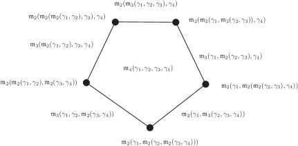
Figure 1. Stasheff 2-gon

We can continue and obtain a $(k-2)$-parameter family of loops $\mathfrak{m}_{k}(\gamma_{1},\dots,\gamma_{k})$ whose boundary parametrizes the union of the compositions of $\mathfrak{m}_{k_{1}}$ and $\mathfrak{m}_{k_{2}}$ with $k_{1}+k_{2}=k+1$. This is the definition of an $A_{\infty}$ space. Its algebraic analogue is an $A_{\infty}$ algebra, which is defined as follows.

Definition 5.1.

(Stasheff) An $A_{\infty}$ algebra is a graded $\mathbb{F}$ module $C$ together with operations

$$\mathfrak{m}_{k}:\underbrace{C\otimes\dots\otimes C}_{k}\to C$$

of degree $2-k$ for $k=1,2,\dots$ which satisfies the following $A_{\infty}$ relation.

$$0=\sum_{k_{1}+k_{2}=k+1}\sum_{i=1}^{k+1-k_{2}}(-1)^{*}\mathfrak{m}_{k_{1}}(x_{1},\dots,\mathfrak{m}_{k_{2}}(x_{i},\dots,x_{i+k_{2}-1})\dots,x_{k}).$$ (5.1)

Here $*=\deg x_{1}+\dots+\deg x_{i-1}+i-1$.

In Lagrangian Floer theory, we use curved and filtered $A_{\infty}$ algebra (and category) which is different from Definition 5.1 at the following points.

1. The operation $\mathfrak{m}_{0}:\mathbb{F}\to C$ can be non-zero.

2. The coefficient ring $\mathbb{F}$ is the universal Novikov ring $\Lambda_{0}$ and the operations are assumed to preserve the filtration. Moreover $\mathfrak{m}_{0}(1)$ is assumed to be in $C\otimes_{\Lambda_{0}}\Lambda_{+}$.

Let us elaborate on those points. In the case when $\mathfrak{m}_{0}=0$, (5.1) implies $\mathfrak{m}_{1}\circ\mathfrak{m}_{1}=0$. However in the case when $\mathfrak{m}_{0}\neq 0$ it implies

$$(\mathfrak{m}_{1}\circ\mathfrak{m}_{1})(x)=(-1)^{\deg x}\mathfrak{m}_{2}(x,\mathfrak{m}_{0}(1))-\mathfrak{m}_{2}(\mathfrak{m}_{0}(1),x).$$

Therefore $\mathfrak{m}_{0}$ is an obstruction for Lagrangian Floer homology to be well-defined.

The universal Novikov ring has a filtration $\mathfrak{F}^{\lambda}\Lambda_{0}$ which consists of elements $\sum_{i=0}^{\infty}a_{i}T^{\lambda_{i}}$ such that $\lambda_{i}\geq\lambda$ for all $i$ with $a_{i}\neq 0$. The module $C$ over $\Lambda_{0}$ is assumed to be a completion of the free $\Lambda_{0}$ module $\overline{C}\otimes_{R}\Lambda_{0}$. In other words it consists of (infinite) sums $\sum_{i=0}^{\infty}c_{i}T^{\lambda_{i}}$ with $\lim_{i\to\infty}\lambda_{i}=+\infty$, where $c_{i}\in\overline{C}$ and $\overline{C}$ is a free $R$ module. Then we can define a filtration on $C$ in a similar way as the filtration on $\Lambda_{0}$. We call such $C$ a completed free filtered $\Lambda_{0}$ module. We then require the operations to preserve the filtration. We call such $(C,\{\mathfrak{m}_{k}\})$ a (curved) filtered $A_{\infty}$ algebra. The topology induced by the filtration is called the $T$-adic topology.

The relation of an $A_{\infty}$ structure to a perturbation of the structure and to mathematical physics had been known before early 1990’s. (See for example [GS].) We can use it in Lagrangian Floer theory as follows. Let $(C,\{\mathfrak{m}_{k}\})$ be a (curved) filtered $A_{\infty}$ algebra. For $b\in C^{\rm odd}$ with $b\in\mathfrak{F}^{\lambda}C$, $\lambda>0$, we consider the Maurer-Cartan equation:

$$\sum_{k=0}^{\infty}\mathfrak{m}_{k}(b,\dots,b)=0.$$ (5.2)

Note that the term for $k=0$ of left hand side is $\mathfrak{m}_{0}(1)$. Since $\mathfrak{m}_{k}(b,\dots,b)\in\mathfrak{F}^{k\lambda}C$ the left hand side converges in $T$-adic topology.

Suppose $b$ solves (5.2). We define the operations $\mathfrak{m}_{k}^{b}$ by the following formula:

$$\mathfrak{m}_{k}^{b}(x_{1},\dots,x_{k})=\sum_{\ell_{0},\dots,\ell_{k}=0}^{\infty}\mathfrak{m}_{k+\sum\ell_{i}}(b^{\ell_{0}},x_{1},b^{\ell_{1}},\dots,b^{\ell_{k-1}},x_{k},b^{\ell_{k}}).$$ (5.3)

The right hand side converges in $T$-adic topology. It is easy to show that $\{\mathfrak{m}_{k}^{b}\}$ satisfies the $A_{\infty}$-relation (5.1). Moreover the Maurer-Cartan equation (5.2) implies $\mathfrak{m}_{0}^{b}=0$. In particular we have

$$\mathfrak{m}_{1}^{b}\circ\mathfrak{m}_{1}^{b}=0.$$

Thus we can eliminate the ‘curvature’ $\mathfrak{m}_{0}$ by using the solution of Maurer-Cartan equation (5.2).

Filtered $A_{\infty}$ algebras appear in Lagrangian Floer theory as follows.

Theorem 5.2.

([FOOO1, FOOO2, AJ]) Let $L$ be a relatively spin Lagrangian submanifold of a symplectic manifold. Then we can associate a structure of a filtered $A_{\infty}$ algebra to $H(L;\Lambda_{0})$.

The same holds for an immersed Lagrangian submanifold if we replace $H(L;\Lambda_{0})$ by $C(L;\Lambda_{0})$.

We can define a map $H^{\rm odd}(L;\Lambda_{+})\to H^{\rm ev}(L;\Lambda_{+})$ by

$$b\mapsto\sum_{k=0}^{\infty}\mathfrak{m}_{k}(b,\dots,b).$$

This is the map $\mathcal{Q}$ in Theorem 4.3.

Bondal-Kapranov [BK] defined the notion of a DG-category. We can modify it to define a filtered $A_{\infty}$ category as follows.

Definition 5.3.

A curved filtered $A_{\infty}$ category $\mathscr{C}$ is the following:

1. The set of objects $\mathfrak{OB}(\mathscr{C})$ is given.

2. For $c,c^{\prime}\in\mathfrak{OB}(\mathscr{C})$ a graded completed free $\Lambda_{0}$ module $\mathscr{C}(c,c^{\prime})$ is given. This is the set of morphisms.

3. We put

   $$B_{k}\mathscr{C}(c,c^{\prime})=\bigoplus_{c_{0},\dots,c_{k}}\bigotimes_{i=1}^{k}\mathscr{C}(c_{i-1},c_{i}),$$

   where the direct sum is taken over $c_{0},\dots,c_{k}\in\mathfrak{OB}(\mathscr{C})$ such that $c_{0}=c$, $c_{k}=c^{\prime}$. We also put

   $$B_{0}\mathscr{C}(c,c^{\prime})=\begin{cases}0&c\neq c^{\prime},\\ \Lambda_{0}&c=c^{\prime}.\end{cases}$$

   The $\Lambda_{0}$ module homomorphisms

   $$\mathfrak{m}_{k}:B_{k}\mathscr{C}(c,c^{\prime})\to\mathscr{C}(c,c^{\prime})$$

   are given for $k=0,1,2,\dots$. It is called the structure operations. The structure operations are required to preserve filtrations.

4. The $A_{\infty}$ relation (5.1) is satisfied.

A filtered $A_{\infty}$ category is said to be strict if $\mathfrak{m}_{0}=0$. To a curved filtered $A_{\infty}$ category $\mathscr{C}$ we can associate a strict filtered $A_{\infty}$ category $\mathscr{C}_{s}$ as follows. We remark that for $c\in\mathfrak{OB}(\mathscr{C})$ the restriction of $\mathfrak{m}_{k}$ defines a structure of a curved filtered $A_{\infty}$ algebra on $\mathscr{C}(c,c)$. A bounding cochain of $c$ is by definition an element $b$ of $\mathscr{C}^{\rm odd}(c,c)$ such that $b\in\mathfrak{F}^{\lambda}\mathscr{C}(c,c)$ for $\lambda>0$ and $b$ satisfies (5.2).

An object of $\mathscr{C}_{s}$ is a pair $(c,b)$ where $c\in\mathfrak{OB}(\mathscr{C})$ and $b$ is its bounding cochain. The module of morphisms $\mathscr{C}_{s}((c,b),(c^{\prime},b^{\prime}))$ is $\mathscr{C}(c,c^{\prime})$. The structure operations of $\mathscr{C}_{s}$ is defined by modifying the structure operations of $\mathscr{C}$ in the same way as (5.3).

A strict $A_{\infty}$ category such that $\mathfrak{m}_{k}=0$ for $k\neq 1,2$ is called a DG-category.

We can define a notion of a (filtered) $A_{\infty}$ functor between two (filtered) $A_{\infty}$ categories. (See [Fu6, Section 7].)

In Lagrangian Floer theory a filtered $A_{\infty}$ category appears in the following way. Let $(X,\omega)$ be a symplectic manifold. We fix a background class $st\in H^{2}(X;{\mathbb{Z}}_{2})$. We consider a finite set $\mathbb{L}$ of $st$-relatively spin (immersed) Lagrangian submanifolds such that for $L,L^{\prime}\in\mathbb{L}$, $L$ is transversal to $L^{\prime}$.

Theorem 5.4.

There exists a curved filtered $A_{\infty}$ category $\mathfrak{Fuk}(X;\mathbb{L})$ the set of whose objects is $\mathbb{L}$. For $L\in\mathbb{L}$ the curved filtered $A_{\infty}$ algebra $\mathfrak{Fuk}(X;\mathbb{L})(L,L)$ is one in Theorem 5.2.

We can prove Theorem 5.4 from Theorem 5.2 as follows. We consider the disjoint union of the elements of $\mathbb{L}$ and regard it as a single immersed Lagrangian submanifold $\hat{L}$. We apply Theorem 5.2 (Akaho-Joyce’s immersed case) to $\hat{L}$ to obtain a curved filtered $A_{\infty}$ algebra. The structure operations of this curved filtered $A_{\infty}$ algebra induce structure operations of $\mathfrak{Fuk}(X;\mathbb{L})$. See also [AFOOO, Fu13]. We denote by $\mathfrak{Fukst}(X;\mathbb{L})$ the strict category associated to $\mathfrak{Fuk}(X;\mathbb{L})$. Its object is a pair $(L,b)$ where $L\in\mathbb{L}$ and $b$ is its bounding cochain.

Let $(L_{i},b_{i})$ be an object of $\mathfrak{Fukst}(X;\mathbb{L})$ for $i=0,1$. The $\mathfrak{m}_{1}$ operator of $\mathfrak{Fukst}(X;\mathbb{L})$ on $\mathfrak{Fukst}(X;\mathbb{L})((L_{0},b_{0}),(L_{1},b_{1}))$ is by definition

$$x\mapsto\sum_{k,\ell=0}^{\infty}\mathfrak{m}_{k+\ell+1}(b_{0}^{k},x,b_{1}^{\ell}).$$

(See (5.3).) Here $\mathfrak{m}_{k+\ell+1}$ in the right hand side is the structure operation of $\mathfrak{Fuk}(X;\mathbb{L})$. This is the boundary operator $d^{b_{0},b_{1}}$ in Theorem 4.3.

As was mentioned at the end of Section 3, we need a bit more general object than those of $\mathfrak{Fukst}(X;\mathbb{L})$ for various purposes. One is establishing topological field theory picture in Donaldson-Floer theory. The others are for homological mirror symmetry (Section 6) and for Lagrangian correspondence (Section 7). One way to do so is to use the notion of an $A_{\infty}$ module over an $A_{\infty}$ category and to use Yoneda embedding.

Definition 5.5.

Let $\mathscr{C}$ be a filtered $A_{\infty}$ category. A right $A_{\infty}$ module $\mathscr{D}$ over $\mathscr{C}$ associates a chain complex $\mathscr{D}(c)$ to each $c\in\mathfrak{OB}(\mathscr{C})$ and a map

$$\mathfrak{n}_{k}:\mathscr{D}(c)\otimes_{\Lambda_{0}}B_{k}\mathscr{C}(c,c^{\prime})\to\mathscr{D}(c^{\prime})$$ (5.4)

for $k=0,1,\dots$ and $c,c^{\prime}\in\mathfrak{OB}(\mathscr{C})$ with the following properties.

1. $\mathfrak{n}_{0}$ is the boundary operator of $\mathscr{D}(c)$.

2. The following $A_{\infty}$ relation is satisfied.

   $$0= \sum_{k_{1}+k_{2}=k}\mathfrak{n}_{k_{2}}(\mathfrak{n}_{k_{1}}(y;x_{1},\dots,x_{k_{1}});x_{x_{1}+1},\dots,x_{k})$$ (5.5)

   $$+\sum_{k_{1}+k_{2}=k+1}\sum_{i=1}^{k_{1}}(-1)^{*}\mathfrak{n}_{k_{1}}(y;x_{1},\dots,\mathfrak{m}_{k_{2}}(x_{i},\dots,x_{i+k_{2}-1}),\dots,x_{k})$$

   where $*=\deg y+\deg x_{1}+\dots+\deg x_{i-1}+i$.

We can define the notion of a right $A_{\infty}$ module homomorphism between two right $A_{\infty}$ modules and obtain a DG-category whose object is a right $A_{\infty}$ module over $\mathscr{C}$. We denote it by $\mathfrak{RMOD}(\mathscr{C})$.

We can define the notion of an $A_{\infty}$ functor. There exists an $A_{\infty}$ functor from $\mathscr{C}$ to $\mathfrak{RMOD}(\mathscr{C})$ which is an $A_{\infty}$ analogue of the Yoneda embedding, as follows.

Let $c\in\mathfrak{OB}(\mathscr{C})$. We associate a right $A_{\infty}$ module $\mathscr{D}_{c}$ by

$$\mathscr{D}_{c}(c^{\prime})=\mathscr{C}(c,c^{\prime})$$

and

$$\mathfrak{n}_{k}(y;x_{1},\dots,x_{k})=\mathfrak{m}_{k+1}(y,x_{1},\dots,x_{k})$$

Here the left hand side is the right module structure and the right hand side is the structure operation of $\mathscr{C}$. The equality (5.5) is a consequence of (5.1).

This is the way how the objects are sent by the Yoneda functor. We can define the morphism part by using the structure operations $\mathfrak{m}$ of $\mathscr{C}$. See [Fu6, Section 9].

An $A_{\infty}$ analogue of Yoneda’s lemma is Theorem 5.7.

Definition 5.6.

A strict unit of an $A_{\infty}$ category $\mathscr{C}$ assigns ${\bf e}_{c}\in\mathscr{C}(c,c)$ (of degree $0$) to each object $c$ such that:

1. $\mathfrak{m}_{k}(\dots,{\bf e}_{c},\dots)=0$ unless $k=2$.

2. $\mathfrak{m}_{2}({\bf e}_{c},x)=(-1)^{*}\mathfrak{m}_{2}(x,{\bf e}_{c})=x$, where $*=\deg x$.

An $A_{\infty}$ category is said to be unital if it has a strict unit.

Theorem 5.7.

If $\mathscr{C}$ is a strict and unital filtered $A_{\infty}$ category, then the Yoneda embedding $\mathscr{C}\to\mathfrak{RMOD}(\mathscr{C})$ is a homotopy equivalence to a full subcategory.

See [Fu6, Fu13] for the homotopy equivalence of filtered $A_{\infty}$ category. See [Fu6, Section 9] for the proof of Theorem 5.7.

By Theorem 5.7 we may regard an object of $\mathscr{C}$ as a right $\mathscr{C}$ module. In other words a right $\mathscr{C}$ module is regarded as an ‘extended’ object of $\mathscr{C}$. Based on this observation the following is proposed in [Fu2, Fu4].

Conjecture 5.8.

([Fu2, Fu4]) Let $M$ be a 3-dimensional manifold with boundary $\Sigma$ and $\mathcal{E}_{M}$ an $SO(3)$ bundle such that $w_{2}(\mathcal{E}_{\Sigma})=[\Sigma]$. (Here $\mathcal{E}_{\Sigma}$ is the restriction of $\mathcal{E}_{M}$ to $\Sigma$.)

Then we can associate a right filtered $A_{\infty}$ module $HF_{M}$ on $\mathfrak{Fukst}(R(\Sigma;\mathcal{E}_{\Sigma});\mathbb{L})$ for any finite set $\mathbb{L}$ of Lagrangian submanifolds of $R(\Sigma;\mathcal{E}_{\Sigma})$.

Furthermore the following holds. Let $M_{i}$ be a 3-dimensional manifold for $i=1,2$ with $\partial M_{i}=\Sigma$ and $\mathcal{E}_{M_{i}}$ an $SO(3)$ bundle such that $w_{2}(\mathcal{E}_{\Sigma})=[\Sigma]$ where $\mathcal{E}_{\Sigma}$ is the restriction of $\mathcal{E}_{M_{i}}$ to $\Sigma$. Let $M$ be a closed $3$-dimensional manifold obtained by gluing $-M_{1}$ and $M_{2}$ along $\Sigma$. An $SO(3)$ bundle $\mathcal{E}_{M}$ on $M$ is obtained by gluing $\mathcal{E}_{M_{1}}$ and $\mathcal{E}_{M_{2}}$. Then we can choose $\mathbb{L}$ such that the isomorphism

$$I(M;\mathcal{E}_{M})\cong H(Hom(HF_{M_{1}},HF_{M_{2}}))$$

holds. Here the left hand side is the instanton Floer homology and the right hand side is the cohomology of the morphism complex in the DG-category of right filtered $A_{\infty}$ modules.

Together with A. Daemi and M. Lipyanskiy the author is on the way of proving this conjecture. (We will discuss it more in Section 7.)

Note that the right $A_{\infty}$ module $HF_{M}$ is supposed to associate a cohomology to an object $(L,b)$ of $\mathfrak{Fukst}(R(\Sigma;\mathcal{E}_{\Sigma});\mathbb{L})$, that is, a pair of a Lagrangian submanifold $L\in\mathbb{L}$ of $R(\Sigma;\mathcal{E}_{\Sigma})$ and its bounding cochain $b$. Let us write it as $HR(M;(L,b))$. An idea in [Fu2, Fu4] for the construction of such cohomology theory $HR(M;(L,b))$ is to study gauge theory of $M\times{\mathbb{R}}$, which has a boundary $\Sigma\times{\mathbb{R}}$ and ends $M\times\{\pm\infty\}$, use $L$ to set an appropriate boundary condition on $\Sigma\times{\mathbb{R}}$, and try to imitate the construction of instanton Floer homology, which is the case $\partial M=\emptyset$.

This part of the idea is later realized in the case when $L$ is monotone and $b=0$ by Salamon-Wehrheim in [SW]. Namely they construct such a Floer homology $HR(M;L)$ of $M$ with coefficient $L$, a monotone Lagrangian submanifold of $R(\Sigma;\mathcal{E}_{\Sigma})$.

To prove the first part of Conjecture 5.8 we also need to define a right module structure, the structure map (5.4). See [Fu12] on this point.

6. Homological Mirror symmetry.

Kontsevich [Ko1] used $A_{\infty}$ categories to formulate his famous homological mirror symmetry conjecture. Actually he used derived category of $A_{\infty}$ categories which we review below.

Let $\mathscr{C}$ be a strict (filtered) $A_{\infty}$ category. We assume for simplicity that for an object $c$ of $\mathscr{C}$ its degree shift $c[k]$ is also exists as an object of $\mathscr{C}$. We consider a finite sequence $c_{1},\dots,c_{n}$ of objects of $\mathscr{C}$ and let $x_{ij}\in\mathscr{C}(c_{i},c_{j})$ for $i<j$. We call $\mathcal{C}=(\{c_{i}\},\{x_{ij}\})$ a twisted complex if for all $i<j$ the next equation is satisfied.

$$\sum\mathfrak{m}_{k}(x_{\ell_{0}\ell_{1}},\dots,x_{\ell_{k-1}\ell_{k}})=0$$ (6.1)

where the sum is taken over the set of all $\ell_{0},\dots,\ell_{k}$ with $k=1,2,\dots$, $\ell_{0}=i$, $\ell_{k}=j$, $\ell_{0}<\dots<\ell_{k}$. Generalizing a similar notion in the case of DG category (which is due to Bondal-Kapranov) Kontsevich introduced the notion of a twisted complex and showed that there is a triangulated category $\mathbb{D}(\mathscr{C})$ whose object is a twisted complex. A triangulated category is an additive category (that is, the category the set of whose morphisms forms an abelian group) so that for each morphism $f:c\to c^{\prime}$ there is a mapping cone which satisfies appropriate axioms. (See [Ha].)

A morphism between two twisted complexes $\mathcal{C}^{(m)}=(\{c_{i}^{(m)}\},\{x^{(m)}_{ij}\})$ $m=1,2$ is a tuple $(y_{ij})$ such that $y_{ij}\in\mathscr{C}(c_{i}^{(1)},c_{j}^{(2)})$. The differential is defined by $d(y_{ij})=(z_{ij})$ where

$$z_{ij}=\sum\mathfrak{m}_{k+n+1}(x^{(1)}_{\ell_{0}\ell_{1}},\dots,x^{(1)}_{\ell_{k-1}\ell_{k}},y_{\ell_{k}m_{0}},x^{(2)}_{m_{0}m_{1}},\dots,x^{(2)}_{m_{n-1}m_{n}}).$$

Here the sum is taken over all $\ell_{0},\dots,\ell_{k}$, $m_{0},\dots,m_{n}$ with $\ell_{0}=i$, $m_{n}=j$.

The equation (6.1) and the $A_{\infty}$ relation imply that $d\circ d=0$. A closed morphism from $\mathcal{C}^{(1)}$ to $\mathcal{C}^{(2)}$ is an element $(y_{ij})$ such that $d(y_{ij})=0$. For a closed morphism we can define its mapping cone. See [Fu6, Section 6]. We can then define a triangulated category $\mathbb{D}(\mathscr{C})$ as the localization of this category so that a closed morphism which induces an isomorphism on cohomologies becomes an isomorphism.

For a complex manifold $X$ we can define an abelian category $\mathscr{SH}(X)$ of its coherent sheaves. Its derived category $\mathbb{D}(\mathscr{SH}(X))$ is defined roughly as follows. (See [Ha].) We consider the additive category whose object is a chain complex of coherent sheaves. We can define mapping cone of such chain complex and also define the notion of a weak equivalence and take the localization. We thus obtain $\mathbb{D}(\mathscr{SH}(X))$.

The homological mirror symmetry conjecture by Kontsevich is stated as:

$$\mathbb{D}(\mathfrak{Fukst}(X))\cong\mathbb{D}(\mathscr{SH}(X^{\vee})),$$ (6.2)

where $X^{\vee}$ is a mirror of $X$.

We can formulate the homological mirror symmetry conjecture using the terminology of filtered $A_{\infty}$ category rather than using that of derived category as follows. Note that the filtered $A_{\infty}$ category $\mathfrak{Fukst}(X)$ is linear over the universal Novikov ring $\Lambda_{0}$, which is similar to the formal power series ring ${\mathbb{C}}[[T]]$. The ring ${\mathbb{C}}[[T]]$ is regarded as ‘the set of functions’ of a formal neighborhood of $0$ in ${\mathbb{C}}$. We regard the mirror of $X$ as a scheme over ${\mathbb{C}}[[T]]$, that is a formal deformation $X^{\vee}\to{\rm Sp}({\mathbb{C}}[[T]])$. We require that it is a formalization of a maximal degenerate family $\pi:X^{\vee}_{\epsilon}\to D^{2}(\epsilon)$ of, say, Calabi-Yau manifolds. Namely we require:

1. For $q\in D^{2}(\epsilon)\setminus\{0\}$ the fiber $M_{q}:=\pi^{-1}(q)$ is a Calabi-Yau manifold. (A Kähler manifold whose canonical bundle is trivial.)

2. The fiber $M_{0}:=\pi^{-1}(0)$ of $0$ is a normal crossing divisor.

3. There exists a point $p$ in $M_{0}$ where the intersection of a neighborhood $U$ of $p$ in $X^{\vee}$ with $M_{0}$ is bi-holomorphic to

   $$\{(z_{0},\dots,z_{n+1})\mid z_{i}\in D^{2},z_{0}\dots z_{n+1}=0\}.$$

Remark 6.1.

It seems that the third condition is equivalent to the following condition.

1. Let $q_{i}\in D^{2}\setminus\{0\}$ be a sequence converging to $0$ and we use a metric on $M_{q_{i}}=\pi^{-1}(q)$ which is Ricci-flat and has diameter $1$. Then the topological dimension of the Gromov-Hausdorff limit $\lim_{i\to\infty}M_{q_{i}}$ is $n$, the complex dimension of $M_{q_{i}}$.

In fact when (md3) is satisfied, it is expected that the Riemannian manifold $M_{q_{i}}$ is mostly occupied in a small neighborhood of the points $p$ in $X^{\vee}$ as in (md3). (Namely the complement of such a neighborhood has small diameter.)

On the other hand, other than the case of dimension 2 ([GW]) or tori, the relation between (*) and (md3) is not established yet. (See [LiY] for a related recent result.) Gross-Wilson [GW] and Kontsevich-Soibelman [KS1] conjectured that condition (*) is equivalent to a definition of the maximal degenerate point in complex geometry, that is, the monodromy $\rho:H_{N}(M_{q})\to H_{N}(M_{q})$ satisfies $(\rho-{\rm id})^{n-1}\neq 0$ and $(\rho-{\rm id})^{n}=0$. The author does not know the present status of this conjecture.

We consider the $n$-fold (branched) covering ${\rm Sp}({\mathbb{C}}[[T^{1/n}]])\to{\rm Sp}({\mathbb{C}}[[T]])$, which induces $X^{\vee}_{n}\to{\rm Sp}({\mathbb{C}}[[T^{1/n}]])$ via pull back. We consider the category of coherent sheaves on $\mathscr{SH}(X^{\vee}_{n})$ which is ${\mathbb{C}}[[T^{1/n}]]$ linear. Take the inductive limit

$$\mathscr{SH}(X^{\vee}_{\infty}):=\varinjlim\mathscr{SH}(X^{\vee}_{n})$$

which is linear over

$$\Lambda_{0,{\mathbb{Q}}}^{{\mathbb{C}}}:=\left\{\sum a_{i}T^{\lambda_{i}}\in\Lambda_{0}^{{\mathbb{C}}}\mid\lambda_{i}\in{\mathbb{Q}}_{\geq 0}\right\}.$$

We then obtain a DG-category (linear over $\Lambda_{0,{\mathbb{Q}}}^{{\mathbb{C}}}$) whose object is a chain complex of objects of $\mathscr{SH}(X^{\vee}_{\infty})$. We denote it by ${\mathbb{DG}}(\mathscr{SH}(X^{\vee}_{\infty}))$.

In the symplectic side we modify $\mathfrak{Fukst}(X)$ slightly so that it becomes $\Lambda_{0,{\mathbb{Q}}}^{{\mathbb{C}}}$ linear in place of being $\Lambda_{0}^{{\mathbb{C}}}$ linear as follows.

Definition 6.2.

Let $(X,\omega)$ be a symplectic manifold. We assume that the cohomology class $[\omega]$ is in $H^{2}(X;{\mathbb{Z}})$ and take a complex line bundle $\mathfrak{L}$ such that $c_{1}(\mathfrak{L})=[\omega]$. We take a Hermitian connection $\nabla$ of $\mathfrak{L}$ such that $F_{\nabla}=2\pi i\,\omega$. A pair $(\mathfrak{L},\nabla)$ is called a pre-quantum bundle.

Let $L$ be a Lagrangian submanifold of $X$. Since $\omega|_{L}=0$, the restriction of $(\mathfrak{L},\nabla)$ to $L$ is flat. Let ${\rm Hol}_{\nabla}:\pi_{1}(L)\to U(1)$ be the holonomy representation of this flat bundle. We say $L$ is rational if the image of ${\rm Hol}_{\nabla}$ is a finite group.

By modifying the construction of $\mathfrak{Fukst}(X)$ we can define a filtered $A_{\infty}$ category $\mathfrak{Fukst}_{{\mathbb{Q}}}(X)$ such that:

1. An object of $\mathfrak{Fukst}_{{\mathbb{Q}}}(X)$ is a pair of a rational Lagrangian submanifold $L$ of $X$ and its bounding cochain $b$ defined over $\Lambda_{0,{\mathbb{Q}}}^{{\mathbb{C}}}$ (see the explanation below).

2. $\mathfrak{Fukst}_{{\mathbb{Q}}}(X)$ is $\Lambda_{0,{\mathbb{Q}}}^{{\mathbb{C}}}$ linear.

Suppose that $L$ is a rational Lagrangian submanifold. We consider the filtered $A_{\infty}$ algebra $CF(L,L)$. The exponent $\lambda$ in the weight $T^{\lambda}$ appearing in the structure operations of the $A_{\infty}$ structure of $CF(L,L)$ is the symplectic area of a disk $(D^{2},\partial D^{2})\to(X,L)$. Using the rationality it is easy to see that $\lambda\in{\mathbb{Q}}_{>0}$. Therefore the Maurer-Cartan equation (5.2) is defined over $\Lambda_{0,{\mathbb{Q}}}^{{\mathbb{C}}}$. Thus the notion of bounding cochain $b$ defined over $\Lambda_{0,{\mathbb{Q}}}^{{\mathbb{C}}}$ makes sense.

We can then modify the definition of $A_{\infty}$ operations slightly so that (2) is satisfied. See [Fu9, Proposition 2.2].

Conjecture 6.3.

There exists a filtered $A_{\infty}$ functor $\mathfrak{Fukst}_{{\mathbb{Q}}}(X)\to{\mathbb{DG}}(\mathscr{SH}(X^{\vee}_{\infty}))$ which induces an isomorphism of their derived categories in certain cases.

6.1. Elliptic curves and tori

The first example of homological mirror symmetry is the case of elliptic curves and is discovered by Kontsevich [Ko1]. He considered three Lagrangian submanifolds $L_{0}$, $L_{1}$, $L_{2}$ in $T^{2}$ (Figure 2).

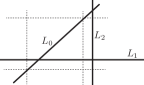
Figure 2. Universal cover of an elliptic curve and its three Lagrangians

In the mirror, $L_{0}$, $L_{1}$ and $L_{2}$ correspond to the structure sheaf, the ample line bundle $\mathscr{O}(1)$ and a point (sky scraper sheaf) $p\in T^{2}$, respectively.

Kontsevich calculated the operation

$$\mathfrak{m}_{2}:HF(L_{0};L_{1})\otimes HF(L_{1};L_{2})\to HF(L_{0};L_{2}).$$ (6.3)

In our situation $HF(L_{0};L_{1})$, $HF(L_{1};L_{2})$, $HF(L_{0};L_{2})$ are all rank one and so (6.3) is a number. We move $L_{2}$ without changing its direction. We also put a flat $U(1)$ connection. These two operations give a family parametrized by one complex number, which becomes a coordinate of the (universal cover of the) mirror elliptic curve.

By definition, the map (6.3) is obtained by counting holomorphic triangles bounding $L_{0}$, $L_{1}$, $L_{2}$ together with an appropriate weight. In our 1-dimensional case, we can calculate it explicitely and there is exactly one such a triangle in each homotopy class, which corresponds one to one to the natural numbers $k$. The symplectic area of the triangle is

$$\frac{(k+c)^{2}}{2}$$

where $c$ is a parameter of $L_{2}$. Thus Kontsevich obtained the theta series:

$$\sum_{k}\exp\left(-\frac{(k+z)^{2}}{2}\right)$$

where $z$ is the coordinate which parametrizes a pair of $L_{2}$ and a flat $U(1)$ connection on it.

In the mirror (6.3) should be

$$H_{\overline{\partial}}(T^{2};\mathscr{O}(1))\otimes_{{\mathbb{C}}}{\mathbb{C}}\to\mathscr{O}(1)_{p}$$

where $p$ is the point corresponding to $z$. Moving $p$, the family of the above operations should be the value of a global section of $\mathscr{O}(1)$ at $p$, which is exactly the theta function. This interesting calculation provides a nice evidence of homological mirror symmetry.

Later Polishchuk and Zaslow [PZ] studied the case of an elliptic curve in more detail and proved the homological mirror symmetry (in the cohomology level) in that case. Their results are partially generalized in [Fu7] to higher dimension, using the idea of family Floer homology (See Section 6.4).

Abouzaid-Smith [ASm] uses the fact that $\mathfrak{Fukst}(T^{2}\times T^{2})$ is related to the category of filtered $A_{\infty}$ functors $\mathfrak{Fukst}(T^{2})\to\mathfrak{Fukst}(T^{2})$ (See Section 7) to prove the homological mirror symmetry for a certain $T^{4}$.

6.2. Generator of the Category 1: Decomposition of the monodromy.

One difficulty in studying homological mirror symmetry is that categories are not easy to study or describe. In fact, usually category is too huge to ‘calculate’. A way to ‘calculate’ an $A_{\infty}$ category is to find its generator and to compute the Floer homology groups between generators together with the structure operations. This is the way how homological mirror symmetry have been proved in many cases. We will discuss two of the methods to find a generator of an $A_{\infty}$ category $\mathfrak{Fukst}(X)$ of symplectic side.

The first one is used in [Se5]. Seidel’s paper [Se5] studies the case of the quartic surface. However his method is applied in greater generality. Let us consider a family of Calabi-Yau manifolds:

$$\pi:\mathfrak{X}\to S^{2}.$$ (6.4)

We consider its restriction

$$\pi:\pi^{-1}(D^{2}(\epsilon))\to D^{2}(\epsilon)$$

to a neighborhood of $0$ and assume that it is a maximal degeneration family, that is, it satisfies (md1), (md2), (md3) above. Take $q\in D^{2}(\epsilon)\setminus\{0\}$. The monodromy around the singular fiber $M_{0}=\pi^{-1}(0)$ defines a symplectic diffeomorphism $\Phi:M_{q}\to M_{q}$, where $M_{q}=\pi^{-1}(q)$. Seidel’s work is based on the following three points.

1. One can define a ${\mathbb{Z}}$-grading on the Floer homology for a certain class of Lagrangian submanifolds in $M_{q}$.

2. For $L$ in such a class and $d\in{\mathbb{Z}}$ the elements of Floer homology $HF(L;\Phi^{k}(L))$ have degree $<d$ for sufficiently large $k$.

3. $\Phi$ is Hamiltonian isotopic to a composition of finitely many Dehn twists around Lagrangian spheres in $M_{q}$.

A brief explanation of them are in order. We first explain (Sei3). For a 2-dimensional manifold $\Sigma$ and a closed loop $\gamma\subset\Sigma$ we can associate a diffeomorphism, the Dehn twist, $D_{\gamma}:\Sigma\to\Sigma$, which is $[C]\mapsto[C]-([\gamma]\cap[C])[\gamma]$ in homology. (Figure 3.)

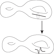
Figure 3. Dehn twist

Its higher dimensional analogue is a symplectic diffeomorphism, the Dehn twist, $\varphi_{S}:X\to X$ associated to a Lagrangian sphere $S^{n}$ in $2n$-dimensional symplectic manifold $X$. In ($n$-dimensional) homology, it is again $[C]\mapsto[C]-([S^{n}]\cap[C])[S^{n}]$. Seidel used the fact that the monodromy of $M_{q}$ is decomposed into a composition of Dehn twists obtained by various Lagrangian spheres in $M_{q}$. The reason of this decomposition is as follows.

We consider a fibration (6.4), which we call a Lefschetz fibration. We study the critical value of $\pi$. One critical value is $0\in S^{2}$. By Assumption (md3), the fiber $M_{0}$ is much degenerate. On the contrary, we can require that the other singular fibers $M_{q_{i}}$ are mildly degenerate. Namely we assume $M_{q_{i}}$ is an immersed submanifold with one transversal self-intersection point. It is a consequence of classical Picard-Lefschetz theory that in such a case there exists a Lagrangian sphere $S_{i}^{n}$ and the monodromy around $q_{i}$ (that is $M_{q}\to M_{q}$ where $q$ is close to $q_{i}$) is a Dehn twist $\varphi_{S^{n}_{i}}$. Thus the monodromy $\varphi$ around $0$ is decomposed into the composition of Dehn twists $\varphi_{S^{n}_{i}}$.

In [Se3] Seidel calculated how the Dehn twist $\varphi_{S}$ acts on the $A_{\infty}$ category $\mathfrak{Fukst}(X)$. It is described by the following long exact sequence:

$$\to HF(\varphi_{S}(L),L^{\prime})\to HF(L,L^{\prime})\to HF(L,S)\otimes HF(S,L^{\prime})\to$$ (6.5)

We consider the ‘difference’ between two objects $L$ and $\varphi_{S}(L)$. Via Yoneda embedding we regard them as right modules over $\mathfrak{Fukst}(X)$. To a Lagrangian submanifold $L^{\prime}$ (which plays the role of a ‘test function’) the difference becomes

$$L^{\prime}\mapsto HF(L,S)\otimes HF(S,L^{\prime}).$$

So it is contained in the subcategory generated by $L^{\prime}\to HF(S,L^{\prime})$, that is, $S$ itself. In this way, together with (Sei2) (Sei3), the exact sequence (6.5) shows that the set of Lagrangian spheres $S^{n}_{q_{i}}$ generates $\mathfrak{Fukst}(X)$.

Remark 6.4.

We remark that (6.5) is related to Floer’s Dehn surgery triangle [Fl7] via Atiyah-Floer conjecture.

Remark 6.5.

We also remark that the above mentioned method is a part of the important project to calculate Floer homology of Lagrangian submanifolds based on symplectic Lefschetz fibration [D5].

Note that in (Sei2) ${\mathbb{Z}}$-grading of Lagrangian Floer homology plays an essential role. We can define such ${\mathbb{Z}}$-grading in the case of a Lagrangian submanifold with vanishing Maslov index as follows ([Se1]). For a positive integer $n$ we consider ${\mathbb{C}}^{n}$ with standard symplectic form $\sum dx_{i}\wedge dy_{i}$ (where $z_{i}=x_{i}+\sqrt{-1}y_{i}$ is the standard coordinate.) We denote by $\mathcal{LAG}({\mathbb{C}}^{n})$ the set of all oriented $n$-dimensional real linear subspaces $V$ of ${\mathbb{C}}^{n}$ such that $\sum dx_{i}\wedge dy_{i}$ is $0$ on $V$. The manifold $\mathcal{LAG}({\mathbb{C}}^{n})$ is called the oriented Lagrangian Grassmannian. Let $X$ be a symplectic manifold. For each $p\in X$ the tangent space $T_{p}X$ is identified with ${\mathbb{C}}^{n}$. (The identification respects the symplectic forms.) We collect $\mathcal{LAG}(T_{p}X)$ for all $p\in X$ and denote it by $\mathcal{LAG}(TX)$. The space $\mathcal{LAG}(TX)$ has a structure of a smooth manifold. There is a smooth map $\mathcal{LAG}(TX)\to X$ which sends $\mathcal{LAG}(T_{p}X)$ to $p$. This map gives a structure of a smooth fiber bundle on $\mathcal{LAG}(TX)$ over $X$. It is well known that $\pi_{1}(\mathcal{LAG}(T_{p}X))={\mathbb{Z}}$. Let $K_{X}$ be the complex line bundle, the $n$-th exterior power of the tangent bundle and $SK_{X}$ its unit circle bundle. There is a bundle map $\mathcal{LAG}(TX)\to SK_{X}$ which associates $[v^{*}_{1}\wedge\dots\wedge v^{*}_{n}]$ to $V\in\mathcal{LAG}(TX)$, where $(v_{1},\dots,v_{n})$ is an oriented basis of $V$ and $v^{*}_{i}$ is its dual basis. The next diagram commutes.

$$\begin{CD}\pi_{1}(\mathcal{LAG}(T_{p}X))@ >>>\pi_{1}(\mathcal{LAG}(TX))@ >>>\pi_{1}(X)\\ @ VVV@ VVV@ VVV\\ \pi_{1}(S^{1})@ >>>\pi_{1}(SK_{X})@ >>>\pi_{1}(X)\end{CD}$$ (6.6)

Moreover the left vertical arrow is an isomorphism.

We assume that $X$ is Calabi-Yau. Therefore $K_{X}$ is the trivial bundle. It follows from the diagram that there exists $\pi_{1}(\mathcal{LAG}(TX))\to{\mathbb{Z}}$ which is an isomorphism on $\pi_{1}(\mathcal{LAG}(T_{p}X))$. Therefore there exists a ${\mathbb{Z}}$ fold cover $\tilde{\mathcal{LAG}}(TX)$ of $\mathcal{LAG}(TX)$ which restricts to the universal cover on each $\mathcal{LAG}(T_{p}X)$.

Let $L$ be an oriented Lagrangian submanifold of $X$. The association $p\mapsto T_{p}L$ defines a section of $\mathcal{LAG}(TX)|_{L}$, which we denote by $s_{L}$. We can show that there exists a section $\tilde{s}_{L}$ of $\tilde{\mathcal{LAG}}(TX)|_{L}$ which lifts $s_{L}$ if and only if the Maslov index of $L$ is zero. We call the lift $\tilde{s}_{L}$ the grading of $L$. The graded Lagrangian submanifold is a pair $(L,\tilde{s}_{L})$. See [Se1]. It is proved there that for a pair of graded Lagrangian submanifolds $(L_{i},\tilde{s}_{L_{i}})$, $i=1,2$, we can define a ${\mathbb{Z}}$ grading of elements $p\in L_{1}\cap L_{2}$ which induces a ${\mathbb{Z}}$ grading of Floer homology.

We do not discuss the proof of (Se2) here.

The method of [Se5] is expanded by various authors and produced various examples where homological mirror symmetry is proved. One important recent development is [She1].

6.3. Generator of the Category 2: Open-closed map.

Before explaining the second method, we recall the notion of a split generation of an $A_{\infty}$ category. Let $\mathscr{C}$ be an $A_{\infty}$ category. We enhance the set of objects of $\mathscr{C}$ in the following three ways.

1. If $c$ is an object of $\mathscr{C}$ and $k\in{\mathbb{Z}}$ we include an object $c[k]$, its degree shift, such that

   $$\mathscr{C}^{d}(c[k],c^{\prime})=\mathscr{C}^{d-k}(c,c^{\prime})\qquad\mathscr{C}^{d}(c^{\prime},c[k])=\mathscr{C}^{d+k}(c^{\prime},c).$$

   The (higher) composition of morphisms between shifted objects is the same as those before shifted except the sign. The sign is determined for example if $xs\in\mathscr{C}(c[1],c^{\prime})$ which is identified with $x\in\mathscr{C}(c,c^{\prime})$ then $\mathfrak{m}_{2}(xs,y)=(-1)^{\deg y+1}\mathfrak{m}_{2}(x,y)s$. Here $s$ is an operator which shifts the degree by $1$.

2. If $c,c^{\prime}$ are objects and $x\in\mathscr{C}(c,c^{\prime})$ is a closed morphism, we include the mapping cone of $x:c\to c^{\prime}$ as an object. (We can do so in the $A_{\infty}$ category of twisted complexes.)

3. We include ‘direct summand’ of an object as a new object. We can do so by using the notion of an idempotent. See [Se4, Section 4].

For any $A_{\infty}$ category $\mathscr{C}$ we can repeatedly add objects by one of the above three operations. We denote by $\mathscr{C}^{+}$ the $A_{\infty}$ category obtained in this way.

Definition 6.6.

Let $X$ be a symplectic manifold and $\mathbb{L}$ a finite set of relatively spin Lagrangian submanifolds. We say $\mathbb{L}$ is a split generator if the following holds.

Let $L^{\prime}$ be an arbitrary relatively spin Lagrangian submanifold. We put $\mathbb{L}^{\prime}=\mathbb{L}\cup\{L^{\prime}\}$. We obtain a filtered $A_{\infty}$ category $\mathfrak{Fukst}(\mathbb{L})$ (resp. $\mathfrak{Fukst}(\mathbb{L}^{\prime})$) whose objects are pairs $(L,b)$ such that $L\in\mathbb{L}$ (resp. $L\in\mathbb{L}^{\prime}$) and $b$ is a bounding cochain of $L$ (resp. $L^{\prime}$).

We change the coefficient ring from $\Lambda_{0}$ to $\Lambda$ to obtain filtered $A_{\infty}$ categories $\mathfrak{Fukst}(\mathbb{L})_{\Lambda}$ and $\mathfrak{Fukst}(\mathbb{L}^{\prime})_{\Lambda}$.

Then by adding objects as in (spg1), (spg2), (spg3) we obtain fitered $A_{\infty}$ categories $\mathfrak{Fukst}(\mathbb{L})_{\Lambda}^{+}$ and $\mathfrak{Fukst}(\mathbb{L}^{\prime})_{\Lambda}^{+}$.

Now we require that the canonical embedding

$$\mathfrak{Fukst}(\mathbb{L})_{\Lambda}^{+}\to\mathfrak{Fukst}(\mathbb{L}^{\prime})_{\Lambda}^{+}$$ (6.7)

is a homotopy equivalece of categories.

The second method to find a generator has an origin in the following proposal (due to Kontsevich). Let $(X,\omega)$ be a symplectic manifold. We consider the product $X\times X$ together with its symplectic form $-\pi_{1}^{*}\omega+\pi_{2}^{*}\omega$, which we denote by $-X\times X$. The diagonal $\Delta=\{(x,x)\in-X\times X\mid x\in X\}$ is a Lagrangian submanifold of $-X\times X$ and $(\Delta,0)$ is an object of $\mathfrak{Fukst}(-X\times X)$.

Suppose that $\mathbb{L}$ is a finite set of relatively spin Lagrangian submanifolds of $X$. We put

$$\mathbb{L}\times\mathbb{L}=\{L\times L^{\prime}\subset-X\times X\mid L,L^{\prime}\in\mathbb{L}\}.$$

We also put $(\mathbb{L}\times\mathbb{L})^{\prime}=(\mathbb{L}\times\mathbb{L})\cup\{\Delta\}.$ We define:

$$\mathfrak{Fukst}(\mathbb{L}\times\mathbb{L})_{\Lambda}^{+}\to\mathfrak{Fukst}((\mathbb{L}\times\mathbb{L})^{\prime})_{\Lambda}^{+}$$ (6.8)

in the same way as (6.7).

The proposal claims that if (6.8) is a homotopy equivalence then $\mathbb{L}$ is a split generator.

One can justify this proposal by using Lagrangian correspondence as follows. As we will explain in Section 7, a Lagrangian submanifold $\mathfrak{L}$ of $-X\times X$ together with its bounding cochain $\mathfrak{b}$ defines a filtered $A_{\infty}$ functor

$$\mathcal{W}_{(\mathfrak{L},\mathfrak{b})}:\mathfrak{Fukst}(X)\to\mathfrak{Fukst}(X).$$

In the case $(\mathfrak{L},\mathfrak{b})=(\Delta,0)$ the functor $\mathcal{W}_{(\Delta,0)}$ is the identity functor. On the other hand, it is easy to see that, if $\mathfrak{L}\in\mathbb{L}\times\mathbb{L}$ and $\mathfrak{b}$ is obtained from a pair of bounding cochains of elements of $\mathbb{L}$ (see [Fu13, Section 16]), then the image of the functor $\mathcal{W}_{(\mathfrak{L},\mathfrak{b})}$ is contained in $\mathfrak{Fukst}(\mathbb{L})$. Therefore if (6.8) is a homotopy equivalence then (6.7) is a homotopy equivalence.

The condition that (6.8) is a homotopy equivalence could be rewritten by using the open-closed map $\mathfrak{p}$ as follows. For an $A_{\infty}$ category $\mathscr{C}$ we can define its Hochshild (co)homology $HH(\mathscr{C})$ and cyclic homology $HC(\mathscr{C})$. In the case when $X$ is compact there are maps

$$\mathfrak{q}_{\mathbb{L}}:HQ^{*}(X;\Lambda_{0})\to HH^{*}(\mathfrak{Fukst}(\mathbb{L})),\quad\mathfrak{p}_{\mathbb{L}}:HC_{*}(\mathfrak{Fukst}(\mathbb{L}))\to H_{*}(X;\Lambda_{0}).$$

(See [Fl5, Ko1, Se2, Al, FOOO1, BC].) The map $\mathfrak{q}_{\mathbb{L}}$ is a ring homomorphism from the quantum cohomology $HQ^{*}(X;\Lambda_{0})$ to the Hochshild cohomology. The domain of $\mathfrak{p}_{\mathbb{L}}$ can be taken also as the Hochshild homology $HH_{*}(\mathfrak{Fukst}(\mathbb{L}))$. Then it is dual to $\mathfrak{q}_{\mathbb{L}}$. (See [AFOOO, Ga].) There is a heuristic argument that the condition (6.8) being a homotopy equivalence becomes the following:

1. The unit $1_{X}\in H_{*}(X;\Lambda)$ is contained in the image of $\mathfrak{p}_{\mathbb{L}}\otimes\Lambda$.

Let us explain the relation between the condition ($\star$) on the open-closed map $\mathfrak{p}_{\mathbb{L}}$ and the condition that (6.8) is a homotopy equivalence. Let $(L\times L,b\times b)$ be an object of $\mathfrak{Fukst}(\mathbb{L}\times\mathbb{L})$. Here $L\in\mathbb{L}$ and $b$ is a bounding cochain of $L$. It induces a bounding cochain $b\times b$ of $L\times L$. We simplify the situation and assume that there exist closed morphisms

$$\mathfrak{x}:(L\times L,b\times b)\to(\Delta,0),\quad\mathfrak{y}:(\Delta,0)\to(L\times L,b\times b)$$

such that

$$\mathfrak{m}_{2}^{-X\times X}(\mathfrak{x},\mathfrak{y})=1_{\Delta}.$$ (6.9)

Here $\mathfrak{m}_{2}^{-X\times X}$ is the structure operations of $\mathfrak{Fukst}(-X\times X;(\mathbb{L}\times\mathbb{L})\cup\{\Delta\})$ and $1_{\Delta}=HF(\Delta)\cong H(X)$ is the unit.

The equality (6.9) is a simplified version of the condition that (6.8) becomes a homotopy equivalence of categories.

We assume furthermore that $\mathfrak{x}$ (resp. $\mathfrak{y}$) is represented as $\mathfrak{x}={\rm PD}[p]\in H^{n}(L)\cong H_{0}(L)$, (resp. $\mathfrak{y}={\rm PD}[L]\in H^{0}(L)\cong H_{n}(L)$). Here $p\in L=(L\times L)\cap\Delta$. In this (over)simplified case, the product in the left hand side is defined by the moduli space as in Figure 4 below.

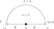
Figure 4. A pseudo-holomorphic map to $-X\times X$.

We (conformally) identify the semi-circle in the figure with a triangle. Three vertices of the triangle are identified with the points $z_{0},z_{1},z_{2}$ in the figure, respectively, and $z_{0}$ is the vertex corresponding to the output. The direct product $u\times u^{\prime}$ is a map from the semi-circle to $-X\times X$ which is required to be pseudo-holomorphic. The part of the boundary of the semi-circle which is the intersection of the semi-circle with $S^{1}$, is required to be mapped to $L\times L$. The other part of the boundary is required to be mapped to the diagonal. The points $z_{1},z_{2}$ are required to be mapped to $(p,p)$ and $L=(L\times L)\cap\Delta$, respectively. (The condition for $z_{2}$ is actually automatic in this case.) We consider the moduli spaces of such maps and use the evaluation map at $z_{0}$. The sum of such output (with appropriate weight) is $\mathfrak{m}_{2}^{-X\times X}(\mathfrak{x},\mathfrak{y})$ by definition. It is a chain of the diagonal $\cong X$.

Now using the fact that the almlost complex structure we use on $-X\times X$ is $-J_{X}\oplus J_{X}$ and $u\times u^{\prime}$ is pseudo-holomorphic, we can use reflexion principle to obtain the map in the Figure 5.

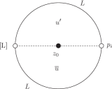
Figure 5. A pseudo-holomorphic map to $X$.

Here $\overline{u}$ is defined by $\overline{u}(z)=u(\overline{z})$. The moduli space of pseudo-holomorphic curves as in Figure 5 is the one we use to define the open-closed map $\mathfrak{p}_{\mathbb{L}}([p]).$ Thus (6.9) is equivalent to $\mathfrak{p}_{\mathbb{L}}([p])=1_{X}.$ It implies ($\star$).

In the more general case where

$$\sum_{i}\mathfrak{p}_{\mathbb{L}}([p_{i,1}]\otimes\dots\otimes[p_{i,k(i)}])=1_{X}$$

the left hand side is obtained from the moduli space depicted by Figure 6. It corresponds to the polygon in Figure 7 (b) on $-X\times X$. This polygon is obtained from the map (6) by reflexion at the dotted line of Figure 7 (a).

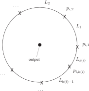
Figure 6. A pseudo-holomorphic map to define the open-closed map.

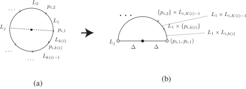
Figure 7. A pseudo-holomorphic polygon obtained by a reflexion.

Abouzaid [Ab2] proved that under the condition ($\star$) (where $H_{*}(X;\Lambda)$ is replaced by the symplectic homology [FH, BO]) $\mathbb{L}$ is a split generator, in a certain non-compact situation. The compact case is on the way being written ([AFOOO]). The proof is based on the Cardy relation [CL] which identifies inner products of cyclic (or Hochshild) homology (See [FOOO6, Shk, AFOOO].) and the Poincaré duality via the open-closed map $\mathfrak{p}$. It does not directly use the above explained idea to relate the condition ($\star$) to (6.8).

As we mentioned already one of the origins of this generating criteria is Kontsevich’s proposal which seems to be related to a similar idea in the study of algebraic cycles in algebraic geometry (via mirror symmetry).

Another origin is in symplectic geometry, such as those in [Al, BC]. It can be stated as follows. Let $L,L^{\prime}$ be two Lagrangian submanifolds of $X$. Suppose

$$\langle\mathfrak{p}(1_{L}),\mathfrak{p}(1_{L^{\prime}})\rangle\neq 0.$$ (6.10)

where $\langle\cdot\rangle:H_{*}(X)\otimes H_{*}(X)\to\Lambda$ is the Poincaré pairing, $\mathfrak{p}$ is the open-closed map and $1_{L}$, $1_{L^{\prime}}$ are the fundamental classes of $L$ and $L^{\prime}$. Then, for any Hamiltonian diffeomorphism $\varphi:X\to X$, we have

$$\varphi(L)\cap L^{\prime}\neq\emptyset.$$ (6.11)

Note that the leading order term of the left hand side of (6.10) (that is, the term which does not contain $T$) is the intersection number $L\cdot L^{\prime}$. So (6.11) is an enhancement of the obvious fact that $L\cdot L^{\prime}\neq 0$ implies $\varphi(L)\cap L^{\prime}\neq\emptyset$.

6.4. Family Floer homology.

Another approach to homological mirror symmetry is by using family Floer homolology. This approach is related to Strominger-Yau-Zaslow’s proposal [SYZ] to construct the mirror manifold via a dual torus fibration. We first briefly review their proposal.

We consider a symplectic manifold $X$ together with a map $\pi:X\to B$, such that for a ‘generic’ point $\mathfrak{b}$ of $B$ the fiber $L_{\mathfrak{b}}:=\pi^{-1}({\mathfrak{b}})$ is a Lagrangian torus. Let $B_{0}\subset B$ be the set of such ‘generic’ points and put $X_{0}=\pi^{-1}(B_{0})$. The tangent space $T_{\mathfrak{b}}B_{0}$ is identified with the first cohomology group $H^{1}(L_{\mathfrak{b}};{\mathbb{R}})$ of the fiber. The group $H^{1}(L_{b};{\mathbb{R}})$ contains a lattice $H^{1}(L_{\mathfrak{b}};{\mathbb{Z}})$. The cotangent fiber $T^{*}_{\mathfrak{b}}B_{0}$ is identified with $H^{1}(L_{\mathfrak{b}};{\mathbb{R}})$ which contains $H^{1}(L_{\mathfrak{b}};{\mathbb{Z}})$. Frequently it is also assumed that $\pi:X\to B$ has a section $s:B\to X$ such that its image is a Lagrangian submanifold. In that case $X_{0}$ is identified with the quotient of $T^{*}_{\mathfrak{b}}B_{0}$ by the lattice $\Gamma:=\cup_{{\mathfrak{b}}\in B_{0}}H^{1}(L_{\mathfrak{b}};{\mathbb{Z}})$. (Here $s(\mathfrak{b})$ becomes $0\in H^{1}(L_{\mathfrak{b}};{\mathbb{R}})/H^{1}(L_{\mathfrak{b}};{\mathbb{Z}})$ by this identification.) Note that the total space of the cotangent bundle has a symplectic structure and the above identification respects the symplectic structures. We consider the fiber-wise dual $TB_{0}$ and its dual lattice $\Gamma^{\vee}$. One can show that the symplectic structure on $T^{*}B_{0}/\Gamma$ induces a complex structure on $TB_{0}/\Gamma^{\vee}$. We put $X_{0}^{\vee}:=TB_{0}/\Gamma^{\vee}$. The complex manifold $X_{0}^{\vee}$ is called a semi-flat mirror to $X_{0}$.

The symplectic structure on $X_{0}$ extends to $X$ (by definition). However the complex structure on $X_{0}^{\vee}$ in general does not extend to its compactification. It is conjectured that there is a ‘quantum correction’ to the complex structure of $X_{0}^{\vee}$ (which is determined by a certain ‘count’ of holomorphic disks bounding a Lagrangian fibers $L_{\mathfrak{b}}$) so that, after correction, the complex manifold $X_{0}^{\vee}$ is compactified to a compact Calabi-Yau manifold $X^{\vee}$ and the map $X_{0}^{\vee}\to B_{0}$ extends to $X^{\vee}\to B$. See [Fu10, KS2, GrS] for example. When a mirror manifold is obtained in this way, $\pi:X\to B$ is called a SYZ-fibration.

The family Floer homology program is a proposal to use SYZ picture of mirror symmetry to produce homological mirror functor $\mathfrak{Fukst}(X)\to{\mathbb{DG}}(\mathscr{SH}(X^{\vee}))$. We consider a Calabi-Yau manifold $X$ together with an SYZ fibration $\pi:X\to B$. We consider a symplectic structure of $X$ only, forgetting its complex structure. (We need an almost complex structure $J$ of $X$ to define the notion of a pseudo-holomorphic curve. However $J$ may not be integrable.) Suppose that we obtain its (SYZ) mirror $X^{\vee}\to B$. $X^{\vee}$ is a Calabi-Yau manifold. We regard it as a complex manifold, forgetting its symplectic structure (that is, the Kähler form).

We consider a Lagrangian submanifold $L$ of $X$. We assume, for simplicity, that $L$ is transversal to the fibers $L_{\mathfrak{b}}:=\pi^{-1}({\mathfrak{b}})$.

A point of $X_{0}^{\vee}$ is a pair of an element $\mathfrak{b}\in B_{0}$ and a cohomology class $a\in H^{1}(T_{\mathfrak{b}};{\mathbb{R}})/H^{1}(T_{\mathfrak{b}};{\mathbb{Z}})$. The class $a$ determines uniquely a flat $U(1)$ bundle $\mathcal{L}_{a}$ on $L_{\mathfrak{b}}$. Let $\mathcal{E}_{L}$ be a vector bundle of $X^{\vee}$ which is the homological mirror to $L$. In this situation, the homological mirror symmetry conjecture ‘implies’:

$$(\mathcal{E}_{L})_{(\mathfrak{b},a)}=HF((L_{\mathfrak{b}},a);L).$$ (6.12)

Here the left hand side is the fiber of the vector bundle and is a ${\mathbb{C}}$-vector space. The right hand side is the Floer homology of $L$ and $L_{\mathfrak{b}}$. The role of $a$ can be explained in two different ways.

1. We regard the right hand side of (6.12) as the Floer homology with local coefficient. Note that the boundary operator of Lagrangian Floer homology is by definition a signed and weighted count of holomorphic strips $u$ with an appropriate boundary condition. (See (4.2) and (path2)’ (path3)’ in Section 4.) We put the weight $T^{\int u^{*}\omega}$ usually. (The variable $T$ is a formal parameter, the Novikov parameter). Here we take the weight $e^{-\int u^{*}\omega}{\rm Hol}_{a}(\partial u)$ instead, where $e$ is the Napier’s number and ${\rm Hol}_{a}(\partial u)$ is the holonomy of the flat line bundle $\mathcal{L}_{a}$ along the loop $u|_{\partial D^{2}}$. (${\rm Hol}_{a}(\partial u)\in U(1)=\{z\in{\mathbb{C}}\mid|z|=1\}$.)

2. We regard $a\in H^{1}(L_{\mathfrak{b}};{\mathbb{R}})\subset H^{1}(L_{\mathfrak{b}};\Lambda_{0})$ and regard it as a bounding cochain as explained in Remark 4.4. Note that $H^{1}(L_{\mathfrak{b}};{\mathbb{R}})/H^{1}(L_{\mathfrak{b}};{\mathbb{Z}})$ which appears in Remark 4.4 is the moduli space of flat $U(1)$ bundle on $L$.

We can then try to use (6.12) as the definition of the vector bundle $\mathcal{E}_{L}$. Namely we conjecture that the $(\mathfrak{b},a)\in X_{0}^{\vee}$-parametrized family of vector spaces $HF((L_{\mathfrak{b}},a);L)$ has a structure of a holomorphic vector bundle on $X_{0}^{\vee}$ that can be extended to $X^{\vee}$.

Note that the Lagrangian submanifold $S=s(B)$ (the image of the Lagrangian section $s$) has the property $HF((L_{\mathfrak{b}},a);S)={\mathbb{C}}$. So we conjecture that it becomes the trivial line bundle (that is, the structure sheaf) of $X^{\vee}$.

The product structure $\mathfrak{m}_{2}$ defines a map

$$HF((L_{\mathfrak{b}},a);S)\otimes HF(S;L)\to HF((L_{\mathfrak{b}},a);L).$$

Since $HF((L_{\mathfrak{b}},a);S)\cong{\mathbb{C}}$ we find that an element of $HF(S;L)$ determines a section of $\mathcal{E}_{L}$. A way to define a holomorphic structure on the family $HF((L_{\mathfrak{b}},a);L)$ is requiring this section to be holomorphic.

The isomorphism $HF^{0}(S;L)\cong H^{0}_{\overline{\partial}}(\mathcal{E}_{L})$ is a part of the claim that $L\mapsto\mathcal{E}_{L}$ defines a fully faithful embedding of $A_{\infty}$ categories.

In [Fu8], the homological mirror symmetry of symplectic and complex tori are proved by this method, in the case when Lagrangian submanifolds $L$ are flat and are transversal to the fibers. A certain discussion in the case when there is a singular fiber and non-flat $L$ can be found in [Fu10].

A few years after [Fu8], Kontsevich-Soibelman [KS1] proposed to use rigid analytic geometry to study homological mirror symmetry and family Floer homology. Note that when we use the weight $e^{-\int u^{*}\omega}{\rm Hol}_{a}(\partial u)$ to define Floer’s boundary operator (and also a similar weight for the structure operations of an $A_{\infty}$ category), it is in general difficult to prove that the series defining the boundary operator etc. converges. In the case of flat Lagrangian submanifolds in symplectic tori, the series defining structure operations are certain variants of the theta series and actually converges very rapidly.

However beyond the case of tori and flat Lagrangian submanifolds, there is no method known to obtain an estimate of the number of holomorphic strips or disks and to show the convergence of the series with weight $e^{-\int u^{*}\omega}{\rm Hol}_{a}(\partial u)$.

In symplectic Floer theory, the usual method is introducing the universal Novikov ring and defining the boundary operator and the structure operations as a ‘formal power series’. Kontsevich-Soibelman [KS1] observed that using the universal Novikov ring in the mirror (complex) side corresponds to studying the mirror manifold as a rigid analytic space. In a series of papers [FOOO3, FOOO4, FOOO6] we worked out the idea using rigid analytic family of Floer homologies to study the case of toric manifolds. Abouzaid [Ab3, Ab4, Ab5] realized this program and proved a version of homological mirror symmetry in the case when the SYZ-fibration $X\to B$ has no singular fiber and the fibers never bound holomorphic disks. J. Tu [Tu] and H. Yuan [Yu] partially relax these conditions and include the case where there exist singular fibers. J. Solomon [So] showed that for the fibers of SYZ-fibration, any $b\in H^{\rm odd}(T^{2n};\Lambda_{0})$ satisfies the Maurer-Cartan equation (5.2).

6.5. Matrix factorizations and weak bounding cochains.

Mirror symmetry is generalized to a manifold $M$ which is not necessary Calabi-Yau. In such a case the mirror of $M$ is not a manifold but is a pair $(M^{\vee},W)$ of a manifold $M^{\vee}$ and a function $W$ on it. Such a mirror symmetry is studied both in the case when $M$ is a symplectic manifold and the case when $M$ is a complex manifold.

We discuss in this subsection the case when $M$ is a symplectic manifold. The other case is discussed in the next subsection. In this case $(M^{\vee},W)$ is a pair of a manifold $M^{\vee}$, and a function $W$ on it. There are cases both $W$ is a holomorphic function and $W$ is a rigid analytic function. For simplicity we explain the case when $M^{\vee}$ is a complex manifold and $W$ is a holomorphic function on it. The function $W$ is called a Landau-Ginzburg potential.

In the Calabi-Yau case, the mirror to the quantum cohomology $HQ(M)$ is the $\overline{\partial}$-cohomology $H_{\overline{\partial}}(M^{\vee},\Lambda^{*}TM^{\vee})$. Here $\Lambda^{*}TM^{\vee}$ is an exterior power of the (complex) tangent bundle of $M^{\vee}$. This cohomology controls the ‘extended’ deformation of the complex structure. In fact, Kodaira-Spencer theory says $H^{1}_{\overline{\partial}}(M^{\vee},TM^{\vee})$ controls the deformation of complex structures of $M^{\vee}$.

In the case when $M$ is not Calabi-Yau, its mirror is a pair $(M^{\vee},W)$. In this case the mirror to the quantum cohomology ring $HQ(M)$ is a vector space which controls the deformation of the pair $(M^{\vee},W)$. In many cases, $W$ has isolated critical points. In such a case, only a neighborhood of the critical point set is used to study the mirror symmetry. So $M^{\vee}$ is a local object (a neighborhood of finitely many points) and has no deformation. The deformation of $W$ is controlled by the Jacobi ring. Let $p\in M^{\vee}$ be a point such that $d_{p}W=0$. We take a complex coordinate $z_{1},\dots,z_{n}$ of $M^{\vee}$ in a neighborhood of $p$. The Jacobi ring $Jac_{p}(W)$ is the quotient:

$$Jac_{p}(W):=\frac{\mathscr{O}_{p}}{\left(\frac{\partial W}{\partial z_{i}}:i=1,\dots,n\right)}.$$ (6.13)

Here $\mathscr{O}_{p}$ is the ring of germs of holomorphic functions of $M^{\vee}$ at $p$. The denominator is its ideal generated by the germs of partial derivatives $\frac{\partial W}{\partial z_{i}}$. In fact the deformation of $W$ (in its first order approximation) can be written as the form

$$t\mapsto W_{t}:=W+tF$$

where $F\in\mathscr{O}_{p}$. Two such deformations $W_{t}$ and $W^{\prime}_{t}$ are regarded as equivalent if there is a family of bi-holomorphic maps $\varphi_{t}$ with $\varphi_{t}(0)=0$ such that $W^{\prime}_{t}\sim W^{\prime}_{t}\circ\varphi_{t}$. It is easy to see that $W+tF$ is equivalent to $W+tF^{\prime}$ if $F-F^{\prime}$ is in the ideal $(\frac{\partial W}{\partial z_{i}}:i=1,\dots,n)$ in its first order approximation. In the case when $p$ is an isolated critical point, the Jacobi ring $Jac_{p}(W)$ is finite dimensional.

K. Saito [Sa] defined an inner-product (higher residue pairing) and various other structures on the (family of) Jacobi rings which is very close to the structure found (by Dubrovin [Dub]) on quantum cohomologies. Such a structure is called a Frobenius manifold structure. These two structures are expected to be identified via mirror symmetry. It seems that among the mathematicians, Givental [Gi] first mentioned this conjecture. The author does not know how this story was developed among physicists.

The homological mirror symmetry between a symplectic manifold $M$ and a pair $(M^{\vee},W)$ is expected to be a relation between a filtered $A_{\infty}$ category $\mathfrak{Fukst}(M)$ and a category of matrix factorizations of $(M^{\vee},W)$. Let us briefly review the notion of a matrix factorization. The notion of a matrix factorization is introduced by Eisenbud [Ei] a long time ago. It is a ${\mathbb{Z}}_{2}$ graded module $C=C_{0}\oplus C_{1}$ over $\mathscr{O}_{p}$ with degree one operator $d:C\to C$ such that

$$d\circ d=W\cdot{\rm Id}.$$ (6.14)

When $(C,d),(C^{\prime},d^{\prime})$ are matrix factorizations we consider the set of $\mathscr{O}_{p}$ module homomorphisms $C\to C^{\prime}$ and denote it by $Hom(C,C^{\prime})$. It is a ${\mathbb{Z}}_{2}$ graded $\mathscr{O}_{p}$ module. We define $\delta:Hom(C,C^{\prime})\to Hom(C,C^{\prime})$ by

$$\delta(\varphi)=d^{\prime}\circ\varphi-(-1)^{\deg\varphi}\varphi\circ d.$$ (6.15)

It is easy to show $\delta\circ\delta=0$. Therefore there exists a DG-categry ${\rm Mat}(W;p)$ whose object is a matrix factorization and the module of morphisms from $(C,d)$ to $(C^{\prime},d^{\prime})$ is $Hom(C,C^{\prime})$, with boundary operator $\delta$ and the obvious composition.

The fact that the matrix factorizations define the D-brane category of the pair $(M^{\vee},W)$ is pointed out by physicists ([KL, HW]) and also in [Or] in early 2000’s.

In Lagrangian Floer theory a similar structure was know by Floer and Oh [Oh] in 1990’s. Let us consider a pair $L_{1}$, $L_{2}$ of monotone Lagrangian submanifolds intersecting transversally. Theorem 4.2 by Oh says if the minimal Maslov number of $L_{1}$ and $L_{2}$ are strictly larger than $2$ then Floer’s boundary operator $d:CF(L_{1},L_{2})\to CF(L_{1},L_{2})$ satisfies $d\circ d=0$. Here $CF(L_{1},L_{2})$ is the free abelian group whose basis is identified with the intersection points.

In the case when the minimal maslov number is $2$, the equality $d\circ d=0$ may not hold. Suppose that the minimal maslov number of a monotone Lagrangian submanifold $L$ is $2$. We consider $\beta\in\pi_{2}(X;L)$ whose Maslov index $\mu(\beta)$ is $2$. Let $\mathcal{M}_{1}(\beta)$ is the moduli space of pseudo-holomorphic maps $u:(D^{2},\partial D^{2})\to(X,L)$ whose homotopy classes are $\beta$. We identify $u$ and $u^{\prime}$ if there exists a biholomorphic map $v:D^{2}\to D^{2}$ such that $u\circ v=u^{\prime}$ and $v(1)=1$. Using the fact that there exists no holomorphic disk whose Maslov index is strictly smaller than $2$, we can show that $\mathcal{M}_{1}(\beta)$ is an $n$-dimensional smooth manifold without boundary for a generic compatible almost complex structure. The map which sends $[u]\in\mathcal{M}_{1}(\beta)$ to $u(1)\in L$ is a smooth map $:\mathcal{M}_{1}(\beta)\to L$ between $n$-dimensional oriented manifolds without boundary and so its mapping degree $n_{\beta}$ is well-defined. We define

$$c_{L}:=\sum_{\beta\in\pi_{2}(X;L),\,\,\,\mu(\beta)=2}n_{\beta}.$$ (6.16)

In the case when $(L_{1},L_{2})$ is a pair of monotone Lagrangian submanifolds intersecting transversally and with the minimal Maslov number $2$, Oh [Oh] proved the following equality:

$$d\circ d=(c_{L_{2}}-c_{L_{1}})\cdot{\rm Id}.$$ (6.17)

The equality (6.17) is the same as (6.14) except $c_{L_{2}}-c_{L_{1}}$ is not a function but is a number (integer).

We can generalize this story without assuming monotonicity as follows. Let $L$ be a relatively spin Lagrangian submanifold of $X$. We obtain a structure of a unital, curved filtered $A_{\infty}$ algebra on $H(L;\Lambda_{0})$. We say $b\in H^{1}(L;\Lambda_{0})$ is a weak bounding cochain if it satisfies:

$$\sum_{k=0}^{\infty}\mathfrak{m}_{k}(b,\dots,b)=c\,\,{\bf e}_{L}$$ (6.18)

for some constant $c\in\Lambda_{0}$. Let $\widetilde{\mathcal{M}}_{\rm weak}(L)$ be the set of all weak bounding cochains of $L$. We define a potential function $\mathfrak{PO}:\widetilde{\mathcal{M}}_{\rm weak}(L)\to\Lambda_{0}$ by

$$\sum_{k=0}^{\infty}\mathfrak{m}_{k}(b,\dots,b)=\mathfrak{PO}(b)\cdot{\bf e}_{L}.$$ (6.19)

Let $(L_{1},L_{2})$ be a transversal pair of relatively spin Lagrangian submanifolds and $b_{i}$ a weak bounding cochain of $L_{i}$ for $i=1,2$. We define $d^{b_{1},b_{2}}:CF(L_{1},L_{2};\Lambda_{0})\to CF(L_{1},L_{2};\Lambda_{0})$ by

$$d^{b_{1},b_{2}}(x):=\sum_{k=0}^{\infty}\sum_{\ell=0}^{\infty}\mathfrak{m}_{k+1+\ell}(b_{1}^{k},x,b_{2}^{\ell}).$$ (6.20)

Here $\mathfrak{m}_{*}$ are the restrictions of the structure operations of the curved $A_{\infty}$ category whose objects are $L_{1}$ and $L_{2}$. Using the $A_{\infty}$ relation and (6.19) we can show ([FOOO1, Proposition 3.7.17]):

$$d^{b_{1},b_{2}}\circ d^{b_{1},b_{2}}=(\mathfrak{PO}(b_{2})-\mathfrak{PO}(b_{1}))\cdot{\rm Id}.$$ (6.21)

This equality shows that $\mathfrak{PO}$ can be regarded as a Landau-Ginzburg potential and $(CF(L_{1},L_{2};\Lambda_{0}),d^{b_{1},b_{2}})$ is identified with the morphism spaces between two matrix factorizations.

Remark 6.7.

Let $(C,d)$, $(C^{\prime},d^{\prime})$ be matrix factorizations with respect to the Landau-Ginzburg potentials $W$, $W^{\prime}$, respectively. We consider $Hom(C,C^{\prime})$ and define the boundary operator $\delta$ by the same formula as (6.15). Then we have $\delta\circ\delta=(W^{\prime}-W)\cdot{\rm Id}$. This formula coincides with (6.21).

Remark 6.8.

In 1990’s Givental gave a comment to a talk by the author that the Landau-Ginzburg potential of the mirror may be obtained as a FOOO’s obstruction class $\mathfrak{m}_{0}$. The author does not know how this story was developed among physicists. It seems that one of its origin is [Wi4]. See also [HIV]. This fact is used in an important paper by Hori-Vafa [HV]. In [HV] this fact is used in the case of certain toric manifolds. Cho-Oh [CO] studied that case and calculated (6.16) in several important toric manifolds. After an important work by Cho [Ch], FOOO [FOOO3, FOOO4, FOOO6] further studied the case of toric manifolds. See also [Au].

The formula (6.21) implies that if $\mathfrak{PO}(b_{1})=\mathfrak{PO}(b_{2})$ the Floer homology group $HF((L_{1},b_{1}),(L_{2},b_{2});\Lambda_{0})$ is defined as the homology group of the boundary operator $d^{b_{1},b_{2}}$. The Floer homology $HF((L_{1},b_{1}),(L_{2},b_{2});\Lambda)$ is expected to be the mirror to the cohomology of the morphism complex of the category of matrix factorizations of $W=\mathfrak{PO}$. We remark that the matrix factorization category of $W$ at $p$ is trivial unless $p$ is a critical point of $W$.

Thus $HF((L_{1},b_{1}),(L_{2},b_{2});\Lambda)$ is expected to be zero unless $b_{1}$, $b_{2}$ are critical points of $\mathfrak{PO}$. We may also expect that the set of critical values of $\mathfrak{PO}$ is a finite set. We define:

$$\mathfrak{C}:=\{c\in\Lambda_{0}\mid\exists(L,b),\,\,b\in\widetilde{\mathcal{M}}_{\rm weak}(L),\,\,\mathfrak{PO}(b)=c,\,\,\,HF((L,b),(L,b);\Lambda)\neq 0\}.$$

Then, for each $c\in\mathfrak{C}$, we can define a strict and unital filtered $A_{\infty}$ category $\mathfrak{Fukst}(X;c)$ so that its object is a pair $(L,b)$ of a Lagrangian submanifold $L$ and its weak bounding cochain $b$ with $\mathfrak{PO}(b)=c$. The structure operations of $\mathfrak{Fukst}(X;c)$ can be defined in the same way as the case of $\mathfrak{Fukst}(X)$, except $\mathfrak{m}_{0}$. Note that $\mathfrak{m}_{0}^{b}(1)=\mathfrak{PO}(b){\bf e}_{(L,b)}\neq 0$. However we redefine $\mathfrak{m}_{0}^{b}$ by putting $\mathfrak{m}_{0}^{b}(1)=0$. In the same way as $\mathfrak{m}_{1}^{b}\circ\mathfrak{m}_{1}^{b}=0$ (which follows from (6.21)) we can check $A_{\infty}$ formula when we redefine $\mathfrak{m}_{0}^{b}(1)$ to be $0$.

Thus, in non-Calabi-Yau cases, we have several strict filtered $A_{\infty}$ categories associated to $X$. In the case of Landau-Ginzburg B-model $(M^{\vee},W)$, there are several matrix factorization categories. Namely for each critical value of $W$ we can associate a category of matrix factorizations. The mirror symmetry is expected to identify them together with decompositions.

Other than the toric case ([FOOO6]), homological mirror symmetry of this type is proved for a certain toric degeneration [NNU1, NNU2] and monotone hypersurfaces of ${\mathbb{C}}P^{n}$ [She2] and etc.

The decompositions of the category are expected to correspond to the decompositions of the quantum cohomology as follows.

Conjecture 6.9.

The quantum cohomology ring $HQ(M,\Lambda)$ is decomposed into the direct product of the rings

$$HQ(M,\Lambda):=\prod_{c\in\mathfrak{C}}HQ(M,\Lambda;c).$$ (6.22)

The closed open map $\mathfrak{q}:HQ(M,\Lambda)\to HH(\mathfrak{Fukst}(X))$ is decomposed into a direct product of the ring homomorphisms:

$$\mathfrak{q}_{c}:HQ(M,\Lambda;c)\to HH(\mathfrak{Fukst}(X);c).$$ (6.23)

We have an equality

$$c_{1}\cup_{q}x=cx$$ (6.24)

for $x\in HQ(M,\Lambda;c)$. Here $c_{1}$ is the first Chern class and $\cup_{q}$ is the quantum cup product.

This conjecture is known to be true in many cases including the case of toric manifolds. It seems unlikely that it is proved in complete generality at the stage when this article is written.

The author heard this conjecture in a lecture by Kontsevich in the year 2006. The author does not know how the story developed among physicists.

Note that in Landau-Ginzburg B-model $(M^{\vee},W)$ the Jacobi ring $Jac(M^{\vee},W)$ is decomposed as:

$$Jac(W)=\prod_{c\in{\rm Crit}(W)}Jac_{c}(W).$$ (6.25)

Here ${\rm Crit}(W)$ is the set of critical values of $W$. If the set of critical points is isolated $J_{c}(W)$ is the direct product of $J_{p}(W)$ for critical points $p$ with $W(p)=c$. If the critical point set is not isolated the story seems to be more involved.

It is expected that the two decompositions (6.22) and (6.25) coincide via mirror symmetry.

6.6. Seidel’s directed $A_{\infty}$ category.

In this subsection, we discuss the mirror symmetry between a complex manifold $M$ and a pair $(M^{\vee},W)$. Here $M$ is not Calabi-Yau. Since the present author is not an expert of this part of homological mirror symmetry, this subsection is rather brief compared to the importance of the topic. When $\mathscr{F}_{i}$, $i=1,2$ are coherent sheaves of $M$, the Serre duality says

$$H^{k}(Hom(\mathscr{F}_{1},\mathscr{F}_{2}))\cong H^{n-k}(Hom(\mathscr{F}_{2},\mathscr{F}_{1})\otimes K_{M}),$$ (6.26)

where $n$ is the complex dimension of $M$ and $K_{M}$ is the canonical bundle, that is, the $n$-th exterior power of complex cotangent bundle of $M$. In the Calabi-Yau case $K_{M}$ is trivial so $H^{k}(Hom(\mathscr{F}_{1},\mathscr{F}_{2}))\cong H^{n-k}(Hom(\mathscr{F}_{2},\mathscr{F}_{1}))$. Note that the Lagrangian Floer homology of compact Lagrangian submanifolds $L_{i}$ satisfies $HF((L_{1},b_{1}),(L_{2},b_{2})))\cong HF((L_{2},b_{2}),(L_{1},b_{1}))$, which is a part of cyclic symmetry and is induced by the Poincaré duality. In the Calabi-Yau case, this is consistent with homological mirror symmetry. However in non-Calabi-Yau case this means that we need to study non-compact Lagrangian submanifolds. Seidel [Se4] defined a directed $A_{\infty}$ category from the pair $(M^{\vee},W)$ (in the exact situation) using a certain set of non-compact Lagrangian submanifolds.

Definition 6.10.

A directed $A_{\infty}$ category $\mathscr{C}$ over $R$ is an $A_{\infty}$ category which is strict, unital and linear over $R$ and such that:

1. The set of its objects consist of finitely many elements $c_{1},\dots,c_{n}$, indexed by a totally ordered set $i=1,\dots,n$.

2. If $i<j$ the set of morphisms $\mathscr{C}(c_{j},c_{i})$ is $\{0\}$.

3. The set of endmorphisms $\mathscr{C}(c_{i},c_{i})$ is $R$ whose basis is the unit.

4. If $i<j$ the set of morphisms $\mathscr{C}(c_{i},c_{j})$ is a finite dimensional free $R$ module.

In complex geometry, an origin of such a directed category is Beilinson’s paper [Be], where the category of coherent sheaves on the projective space $\mathbb{P}^{n}$ is studied. In that case $c_{i}=\mathscr{O}(i)$ for $i=0,\dots,n$ satisfies this condition for $\mathscr{C}(c_{i},c_{j}):=H_{\overline{\partial}}(Hom(c_{i},c_{j}))$. (Here $\mathscr{O}(i)$ is a line bundle of degree $i$.) This set is also a generator of the derived category of coherent sheaves. Such a generator is called a full (strong) exceptional collection (of the category of coherent sheaves). This notion is defined in [GR].

Seidel’s construction is the case when the symplectic manifold $M^{\vee}$ is exact and $W:M^{\vee}\to{\mathbb{C}}$ has a mild singularity, that is, for each critical value $q$, the fiber $M^{\vee}_{q}=W^{-1}(q)$ is an immersed symplectic submanifold with one transversal self-intersection point. The non-compact Lagrangian submanifold Seidel studied is a kind of unstable manifold of $W$ which is called a Lefschetz thimble. For $p\in M^{\vee}$ such that $D_{p}W\neq 0$, decompose the tangent space $T_{p}M^{\vee}$ as $T_{p}M^{\vee}=T^{v}_{p}M^{\vee}\oplus T^{h}_{p}M^{\vee}$ where $T^{v}_{p}M^{\vee}=T_{p}W^{-1}(W(p))$ and $T^{h}_{p}M^{\vee}$ is its orthogonal complement with respect to the symplectic form. Using this decomposition we can define a horizontal lift of a path in ${\mathbb{C}}$. For each critical value $q_{i}\in{\mathbb{C}}$ take a path $\gamma_{i}:[0,\infty)\to{\mathbb{C}}$ such that $\gamma_{i}(0)=q_{i}$ and that, if $t$ is sufficiently large, then $\gamma_{i}(t)=t+\sqrt{-1}C_{i}$ for a certain $C_{i}\in{\mathbb{R}}$, such that it does not intersect with critical values for $t\neq 0$. For $x\in W^{-1}(\gamma_{i}(t_{0}))$ we take a horizontal lift $\widetilde{\gamma}_{x}:[0,t_{0}]\to M^{\vee}$ of $\gamma_{i}$ such that $\widetilde{\gamma}_{x}(t_{0})=x$. We consider the set $L_{i}$ of all $x\in W^{-1}(\gamma_{i}([0,\infty))$ such that $\widetilde{\gamma}_{x}(0)$ is a critical point of $M_{q_{i}}=W^{-1}(q_{i})$. It is known that $L_{i}$ is a Lagrangian submanifold of $M^{\vee}$ and is called a Lefschetz thimble. For each $\gamma_{i}(t_{0})$, $t_{0}\neq 0$ the fiber $W^{-1}(\gamma_{i}(t_{0}))\cap L_{i}$ is known to be a Lagrangian sphere of the symplectic manifold $W^{-1}(\gamma_{i}(t_{0}))$ and is called a vanishing cycle.

We assume that the path $\gamma_{i}$ and $\gamma_{j}$ do not intersect each other for $i\neq j$ and that $C_{i}<C_{j}$ for $i<j$. The Lefschetz thimbles $L_{i}$ $i=1,\dots,n$ do not intersect each other. We will perturb it slightly near the infinity so that they intersect as follows. We take a Hamiltonian $H:M^{\vee}\to{\mathbb{R}}$ such that $H(x)=\epsilon\|W(x)\|^{2}$. We consider the time one map $\varphi_{H}$ of the Hamiltonian vector field $\mathfrak{X}_{H}$. The map $\varphi_{H}$ rotates the image of $\gamma_{i}$ slightly to the counter clockwise direction so that $\varphi_{H}(L_{i})\cap L_{j}\neq\emptyset$ if and only if $i<j$. We put

$$\mathscr{S}(L_{i},L_{j})=CF(\varphi_{H}(L_{i}),L_{j}),$$

where the right hand side is the usual Floer complex. This is zero if $j<i$ and so (6.10) is satisfied. For $i=j$ we define $\mathscr{S}(L_{i},L_{i})=R$, the ground ring. Under a certain exactness assumption on the symplectic form and a certain condition on the behavior of $W$ near infinity, Seidel defined a directed $A_{\infty}$ category $\mathscr{S}(M^{\vee},W)$ the set of whose objects are $\{L_{i}\mid i=1,\dots,n\}$ and the morphism complex is $\mathscr{S}(L_{i},L_{j})$.

It is possible to increase objects by requiring the Lagrangian submanifold to have an asymptotic behavior similar to $L_{i}$’s. Namely we can consider $L$ such that outside a compact set $L$ is obtained by a parallel transport along an arc $t\mapsto t+C\sqrt{-1}$. (The case of a compact Lagrangian submanifold $L$ is included.)

Remark 6.11.

In place of rotating Lagrangian submanifolds a bit one can take a Hamiltonian such as $\|W(x)\|^{4}$ so that the rotation angle goes $\infty$ as one goes to the infinity of ${\mathbb{C}}$. Abouzaid-Seidel [ASe] defined such an $A_{\infty}$ category which is called a wrapped (Fukaya) category. A wrapped category is related to the symplectic homology in the same way as $\mathfrak{Fukst}(X)$ is related to the quantum cohomology of $X$. Auroux proposed to generalize the notion of a wrapping to a partial wrapping. Ganatra-Pardon-Shande [GPS1, GPS2, GPS3] realized this program suceessfully.

The homological mirror symmetry conjectures that a fully exceptional collection of a, say, Fano manifold $M$ is isomorphic to a version of $\mathscr{S}(M^{\vee},W)$. Seidel first proved it in the case when $M={\mathbb{C}}P^{2}$. It then is generalized to the case of $2$-dimensional weighted projective space (Auroux-Kazarkov-Orlov [AKO2]) and blow up of ${\mathbb{C}}P^{2}$ at $k$ point ($k\leq 3$ by Ueda [Ue] and then $k\leq 8$ by Auroux-Kazarkov-Orlov [AKO1]). It is also proved when $M$ is a toric Fano manifold (Abouzaid [Ab1] and Fang-Liu-Treumann-Zaslov [FLTZ]).

Compared to the story when $M$ is the symplectic side, an issue is that it is not clear how to obtain the function $W$ in a conceptional way. The approach by [AAK] (See also [CLL]) may give a way to do so.

7. Lagrangian correspondence and Gauge theory.

Before discussing further the topological field theory of 2-3-4 dimensional manifolds based on Yang-Mills theory, we describe its ‘finite dimensional analogue’, that is, a Lagrangian correspondence and its relation to Lagrangian Floer theory.

Let $(X,\omega_{X}),(Y,\omega_{Y})$ be symplectic manifolds. We consider the product $X\times Y$ together with the symplectic form $-\pi_{1}^{*}\omega_{X}+\pi_{2}^{*}\omega_{Y}$. We write $-X\times Y:=(X\times Y,-\pi_{1}^{*}\omega_{X}+\pi_{2}^{*}\omega_{Y})$. Weinstein [We] proposed to regard a Lagrangian submanifold of the product $-X\times Y$ as a morphism $X\to Y$ between symplectic manifolds. We call a Lagrangian submanifold of $-X\times Y$ a Lagrangian correspondence.

There are several reasons behind this proposal.

1. We consider a symplectic diffeomorphism $\varphi:X\to Y$ (that is, a diffeomorphism $\varphi$ such that $\varphi^{*}\omega_{Y}=\omega_{X}$.) Then its graph $\{(x,\varphi(x))\mid x\in X\}$ is a Lagrangian submanifold of $-X\times Y$.

2. Let $X_{i}$ be a symplectic manifold for $i=1,2,3$ and $L_{i(i+1)}\subset-X_{i}\times X_{i+1}$ be a Lagrangian submanifold for $i=1,2$. We consider the fiber product:

   $$L_{13}=\{(x,y)\in L_{12}\times L_{23}\mid\pi_{2}(x)=\pi_{1}(y)\},$$

   where for $z=(a,b)\in-X_{i}\times X_{i+1}$ we denote $\pi_{1}(z)=a$, $\pi_{2}(z)=b$. In the generic case, that is, the case when the fiber product is transversal, it is easy to see that $L_{13}$ is a smooth manifold and $L_{13}\to-X_{1}\times X_{3}$, $(x,y)\mapsto(\pi_{1}(x),\pi_{2}(y))$ is a Lagrangian immersion. Thus we can ‘generically’ compose Lagrangian correspondences.

3. Another example of a Lagrangian correspondence is obtained from the symplectic quotient. Suppose $X$ is a symplectic manifold on which a compact Lie group $G$ acts preserving the symplectic structure. We assume that there exists a moment map $\mu:X\to\mathfrak{g}^{*}$, where $\mathfrak{g}^{*}$ is the Lie algebra of $G$. The symplectic quotient $X/\!/G$ is by definition $\mu^{-1}(0)/G$ ([MWe]). If $X/\!/G$ is smooth, it is known that it carries a symplectic form $\overline{\omega}$ whose pullback to $\mu^{-1}(0)$ coincides with the restriction of the symplectic form of $X$.

   Now we consider

   $$L=\{(x,y)\in X\times X/\!/G\mid\mu(x)=0,\,\,[x]=y\}.$$

   This is a Lagrangian submanifold of $-X\times X/\!/G$.

Since this proposal by Weinstein looks so natural, there has been attempts to associate a functor $\mathfrak{F}_{\mathfrak{L}}:\mathfrak{Fukst}(X)\to\mathfrak{Fukst}(Y)$ to a Lagrangian correspondence $\mathfrak{L}$. A possible naive idea to do so is the following. Let $L$ be a Lagrangian submanifold of $X$. Instead of associating an object of $\mathfrak{Fukst}(Y)$ to $L$, we try to define a right $\mathfrak{Fukst}(Y)$-module $\mathfrak{F}_{\mathfrak{L}}(L)$. In the cohomology level, $\mathfrak{F}_{\mathfrak{L}}(L)$ can be defined by associating the Floer homology $HF(\mathfrak{L};L\times L^{\prime})$ in the product $-X\times Y$ to a Lagrangian submanifold $L^{\prime}$ of $Y$. Actually we can construct an $A_{\infty}$ functor:

$$\mathfrak{F}_{\mathfrak{L}}:\mathfrak{Fukst}(X)\to\mathcal{RMOD}(\mathfrak{Fukst}(Y))$$ (7.1)

in this way. (See [Fu13, Section 5] for its rigorous construction.) As we explained in Section 5 of this article, an object of $\mathcal{RMOD}(\mathfrak{Fukst}(Y))$ can be regarded as an ‘extended object’ of $\mathfrak{Fukst}(Y)$ (via Yoneda embedding). Thus (7.1) could be regarded as a version of $\mathfrak{F}_{\mathfrak{L}}:\mathfrak{Fukst}(X)\to\mathfrak{Fukst}(Y)$. However the problem is in this formulation it is difficult to compose $\mathfrak{F}_{\mathfrak{L}_{12}}$ and $\mathfrak{F}_{\mathfrak{L}_{23}}$ where $\mathfrak{L}_{i(i+1)}$ is a Lagrangian submanifold of $-X_{i}\times X_{i+1}$. This situation is somewhat similar to the following: If we are given a current $S$ (that is, a Schwartz kernel) on $M\times N$ and a smooth differential form $u$ on $M$ then we obtain a current $S_{*}(u)$ on $N$ by the equality

$$S_{*}(u)(v)=S(u\times\pi_{2}^{*}(v)).$$ (7.2)

In other words, an object of $\mathfrak{Fukst}$ is an analogy of a smooth differential form and an object of $\mathcal{RMOD}(\mathfrak{Fukst}(Y))$ is an analogy of a distributional form. We use a ‘test Lagrangian’ in place of a ‘test function’. It is difficult to compose two operators of the form (7.2). In this sense, Theorem 7.1 could be regarded as a kind of ‘regularity theorem’.

In [MWW, WW1, WW2, WW4, WW3], Wehrheim-Woodward-Ma’u used the following idea to go around this problem. For a given symplectic manifold $X$, they consider a series of Lagrangian correspondences $L_{i}\subset-X_{i}\times X_{i+1}$ such that $X_{0}$ is a point and $X_{n}=X$. They regard such a system $(L_{0},\dots,L_{n})$ as an object of expanded category $\mathfrak{Fuk}(X)^{+}$. Then, if $\mathfrak{L}\subset-X\times Y$ is a Lagrangian correspondence, one can define

$$(\mathcal{W}_{{\mathfrak{L}}})_{\rm ob}:\mathfrak{OB}(\mathfrak{Fuk}(X)^{+})\to\mathfrak{OB}(\mathfrak{Fuk}(Y)^{+}),$$

by $(L_{0},\dots,L_{n})\mapsto(L_{0},\dots,L_{n},\mathfrak{L})$.

To define the category $\mathfrak{Fuk}(X)^{+}$, one needs to define the Floer homology between extended objects $(L_{0},\dots,L_{n})$, $(L^{\prime}_{0},\dots,L^{\prime}_{n^{\prime}})$, where $L_{i}\subset-X_{i}\times X_{i+1}$ and $L^{\prime}_{i}\subset-X^{\prime}_{i}\times X^{\prime}_{i+1}$, $X_{0},X^{\prime}_{0}$ are points and $X_{n}=X^{\prime}_{n^{\prime}}=X$. They denote this Floer homology by $HF(L_{0},\dots,L_{n},L^{\prime}_{n^{\prime}},\dots,L^{\prime}_{0})$. Wehrheim-Woodward-Ma’u used the notion of a pseudo-holomorphic quilt to define it. Actually their definition is equivalent to the following:

$$HF(L_{0},\dots,L_{n},L^{\prime}_{n^{\prime}},\dots,L^{\prime}_{0}):=HF(L_{0}\times\dots\times L_{n}\times L^{\prime}_{0}\times\dots\times L^{\prime}_{n^{\prime}};\Delta).$$ (7.3)

Here

$$\Delta\subset\left(\prod_{i=1}^{n-1}(-X_{i}\times X_{i})\right)\times\left(\prod_{i=1}^{n^{\prime}-1}(-X^{\prime}_{i^{\prime}}\times X^{\prime}_{i^{\prime}})\right)\times(-X\times X)$$ (7.4)

is the product of diagonals. The right hand side of (7.3) is the Floer homology of two Lagrangian submanifolds in the symplectic manifold given in (7.4).

In the simplest case, a pseudo-holomorphic quilt used to define $HF(L_{0},L_{1},L^{\prime}_{0})$ is a map $u=(u_{1},u_{2})$ from the domain depicted in Figure 8 below.

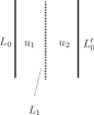
Figure 8. A simplest pseudo-holomorphic quilt.

Here the domain is divided into two parts. The map $u_{1}$ (resp. $u_{2}$) is defined on the left (resp. right) part of the domain and is a pseudo-holomorphic map to $-X_{1}$ (resp. $X$). The boundary conditions are required on the three lines, the left most, the right most and the middle (dotted) lines. The boundary condition for the left most line is $u_{1}(z)\in L_{0}$, one for the right most line is $u_{2}(z)\in L^{\prime}_{0}$. The boundary condition for the middle line is $(u_{1}(z),u_{2}(z))\in L_{1}$. We remark that $L_{1}$ is a Lagrangian submanifold of $-X_{1}\times X$. The middle line is called a seam.

By reflexion principle, $(\overline{u}_{1},u_{2}):[0,1]\to-X_{1}\times X$ is a pseudo-holomorphic map which satisfies the boundary condition given by Lagrangain submanifolds $L_{1}$ and $L_{0}\times L^{\prime}_{0}$. The moduli space of such pseudo-holomorphic maps is used to define $HF(L_{1},L_{0}\times L^{\prime}_{0})$.

The pseudo-holomorphic quilt used to define $HF(L_{0},\dots,L_{n},L^{\prime}_{n^{\prime}},\dots,L^{\prime}_{0})$ is as in Figure 9 below.

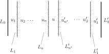
Figure 9. A pseudo-holomorphic quilt.

Here $u_{i}$ (resp. $u^{\prime}_{i}$) is a pseudo-holomorphic map to $-X_{i}$ (resp. $X^{\prime}_{i}$) and $u$ is a pseudo-holomorphic map to $X$.

Wehrheim-Woodward-Ma’u studied the case when all the Lagrangian submanifolds $L_{i}$, $L^{\prime}_{i}$ are monotone. So we can use Oh’s work [Oh] to define it.

In this way [MWW] defined a version of an $A_{\infty}$ bi-functor

$$\mathcal{MWW}:\mathfrak{Fukst}(-X\times Y)\times\mathfrak{Fukst}(X)\to\mathfrak{Fukst}(Y)$$ (7.5)

where all the Lagrangian submanifolds involved are assumed to be monotone and embedded and $\mathfrak{Fukst}(\dots)$ is replaced by $\mathfrak{Fukst}(\dots)^{+}$.

The advantage to use peudo-holomorphic quilt rather than Floer homology in the direct product (as in (7.3)) lies in the fact that, then, one can use ‘strip shrinking’ to prove the next isomorphism

$$HF(L_{0},\dots,L_{n},L^{\prime}_{n^{\prime}},\dots,L^{\prime}_{0})$$ (7.6)

$$\cong HF(L_{0},\dots,L_{n-1},L_{n}\times_{X}L^{\prime}_{n^{\prime}},L^{\prime}_{n^{\prime}-1},\dots,L^{\prime}_{0}).$$

The strip shrinking is a process to change the width between two seams until it becomes $0$. (See Figure 10.) Note that the method of using reflexion principle to replace Wehrheim-Woodward’s definition by (7.3) works only in the case when all the strips have the same width. Therefore it is not consistent with strip shrinking.

Figure 10. Strip shrinking.

[WW1, WW2, WW4, WW3] proved the isomorphism (7.6) under the assumption that all the Lagrangian submanifolds involved (including the fiber product $L_{n}\times_{X}L^{\prime}_{n^{\prime}}$) are embedded and monotone. The isomorphism (7.6) is a version of composability of filtered $A_{\infty}$ functors associated to the composition of Lagrangian correspondences. Later Lekili and Lipyanskiy [LL] found an alternative method, using cobordism argument instead of strip shrinking. For example Lekili-Lipyanskiy’s proof of $HF(L_{0},L_{1},L^{\prime}_{1},L^{\prime}_{0})\cong HF(L_{0},L_{1}\times_{X}L^{\prime}_{1},L^{\prime}_{0})$ uses the moduli space of pseudo-holomorphic curves with the domain depicted by Figure 11 below.

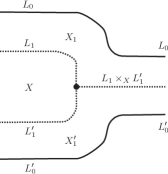
Figure 11. Y Diagram.

The three dotted lines (seams) are required to be mapped to $L_{1}$, $L^{\prime}_{1}$, $L_{1}\times_{X}L^{\prime}_{1}$, respectively. The other two curves are required to be mapped to $L_{0}$ and $L^{\prime}_{0}$. The three domains are required to be mapped to $-X_{1}$, $X^{\prime}_{1}$, $X$ as depicted. The maps on those domains are required to be pseudo-holomorphic. In the left end the pseudo-holomorphic quilt used to define $HF(L_{0},L_{1},L^{\prime}_{1},L^{\prime}_{0})$ appears. In the right end the pseudo-holomorphic quilt used to define $HF(L_{0},L_{1}\times_{X}L^{\prime}_{1},L^{\prime}_{0})$ appears. Lekili and Lipyanskiy called Figure 11 the Y-diagram.

After those works had been done, the author found that the naive idea in 1990’s which we described at the beginning of this section, can be realized using the technology developed in these 20 years and the cobordism argument due to Lekili and Lipyanskiy, as follows.

We consider the filtered $A_{\infty}$ functor (7.1) and also the Yoneda functor:

$$\mathfrak{YON}:\mathfrak{Fukst}(Y)\to\mathcal{RMOD}(\mathfrak{Fukst}(Y)).$$ (7.7)

Theorem 7.1.

([Fu13]) Let $(\mathfrak{L},\mathfrak{b})\in{\mathfrak{OB}}(\mathfrak{Fukst}(-X\times Y))$ and $(L,b)\in\mathfrak{OB}(\mathfrak{Fukst}(X))$ be objects such that the fiber product $L\times_{X}\mathfrak{L}$ is transversal. Then there exists a bounding cochain $b^{\prime}$ of the immersed Lagrangian submanifold $L^{\prime}:=L\times_{X}\mathfrak{L}$ of $Y$ such that $(\mathfrak{YON})_{\rm ob}(L^{\prime},b^{\prime})$ is homotopy equivalent to $(\mathfrak{F}_{\mathfrak{L}})_{\rm ob}(L,b)$.

Theorem 7.1 enables us to obtain a filtered $A_{\infty}$ functor

$$\mathcal{W}_{(\mathfrak{L},\mathfrak{b})}:\mathfrak{Fukst}(X)\to\mathfrak{Fukst}(Y)$$

such that its composition with the Yoneda functor is homotopy equivalent to the functor $\mathfrak{F}_{\mathfrak{L}}$ in (7.1). It is also proved in [Fu13] that $\mathcal{W}_{(\mathfrak{L},\mathfrak{b})}$ is induced from a filtered $A_{\infty}$ bi-functor (7.5), where objects of the categories involved are immersed and unobstructed. (It is unnecessary to assume them to be monotone or embedded.)

The association $(\mathfrak{L},\mathfrak{b})\mapsto\mathcal{W}_{(\mathfrak{L},\mathfrak{b})}$ is functorial. Namely the following is proved in [Fu13]. Let $(\mathfrak{L}_{i(i+1)},\mathfrak{b}_{i(i+1)})\in{\mathfrak{OB}}(\mathfrak{Fukst}(-X_{i}\times X_{i+1}))$ for $i=1,2$. We assume that the fiber product $\mathfrak{L}_{12}\times_{X_{2}}\mathfrak{L}_{23}$ is transversal and put $\mathfrak{L}_{13}=\mathfrak{L}_{12}\times_{X_{2}}\mathfrak{L}_{23}$, which is an immersed Lagrangian submanifold of $-X_{1}\times X_{3}$. Then there exists a bounding cochain $\mathfrak{b}_{13}$ of $\mathfrak{L}_{13}$ such that:

$$\mathcal{W}_{(\mathfrak{L}_{13},\mathfrak{b}_{13})}\sim\mathcal{W}_{(\mathfrak{L}_{23},\mathfrak{b}_{23})}\circ\mathcal{W}_{(\mathfrak{L}_{12},\mathfrak{b}_{12})}$$

where $\sim$ means homotopy equivalent.

In the situation of (Wei3) the Lagrangian correspondence from $X$ to $X/\!/G$ is expected to induce a functor from an equivariant version of $\mathfrak{Fukst}(X)$ to $\mathfrak{Fukst}(X/\!/G)$. Such a functor is studied by Woodward and Xu in [WX]. It is an ‘open string analogue’ of [Wo], based on gauged sigma model (See [CGRS]).

An infinite dimensional version of the situation of (Wei3) appears in gauge theory as follows. Let $\Sigma$ be a Riemann surface and $\mathcal{E}_{\Sigma}$ an $SO(3)$ or $SU(2)$ principal bundle on it. We define $\mathcal{A}(\Sigma;\mathcal{E}_{\Sigma})$ to be the set of all $SO(3)$ or $SU(2)$ connections of $\mathcal{E}_{\Sigma}$. The space $\mathcal{A}(\Sigma;\mathcal{E}_{\Sigma})$ is an affine space and the tangent space of each point is the vector space $\Gamma(\Sigma,\Lambda^{1}\otimes ad\mathcal{E}_{\Sigma})$ of sections. Here $\Lambda^{1}$ is the bundle of 1-forms and $ad\mathcal{E}_{\Sigma}$ is the adjoint bundle associated to $\mathcal{E}_{\Sigma}$. For $V,W\in\Gamma(\Sigma,\Lambda^{1}\otimes ad\mathcal{E}_{\Sigma})$ we put

$$\Omega(V,W)=-\frac{1}{8\pi^{2}}\int_{\Sigma}{\rm Tr}(V\wedge W),$$

which defines a symplectic structure on $\mathcal{A}(\Sigma;\mathcal{E}_{\Sigma})$.

Let $\mathcal{G}(\Sigma;\mathcal{E}_{\Sigma})$ be the gauge transformation group. It is easy to see that the $\mathcal{G}(\Sigma;\mathcal{E}_{\Sigma})$ action on $\Gamma(\Sigma,\Lambda^{1}\otimes ad\mathcal{E}_{\Sigma})$ preserves the symplectic structure. Moreover there is a moment map of this action, which is nothing but the curvature, in the following way. The Lie algebra of the gauge transformation group is $\Gamma(\Sigma,ad\mathcal{E}_{\Sigma})$. We identify its dual with $\Gamma(\Sigma,\Lambda^{2}\otimes ad\mathcal{E}_{\Sigma})$ by

$$V(W)=-\frac{1}{8\pi^{2}}\int_{\Sigma}{\rm Tr}(V\wedge W)$$

where $W\in\Gamma(\Sigma,ad\mathcal{E}_{\Sigma})$ and $V\in\Gamma(\Sigma,\Lambda^{2}\otimes ad\mathcal{E}_{\Sigma})$ in the right hand side and $V$ is a linear map $\Gamma(\Sigma,ad\mathcal{E}_{\Sigma})\to{\mathbb{R}}$ in the left hand side. Thus the moment map is a map $\mu:\mathcal{A}(\Sigma;\mathcal{E}_{\Sigma})\to\Gamma(\Sigma,\Lambda^{2}\otimes ad\mathcal{E}_{\Sigma}).$ One can check that

$$\mu(A)=-\frac{1}{8\pi^{2}}F_{A}.$$

It implies that the symplectic quotient of the $\mathcal{G}(\Sigma;\mathcal{E}_{\Sigma})$ action on $\mathcal{A}(\Sigma;\mathcal{E}_{\Sigma})$ is the set of gauge equivalence classes of the flat connections.

One can also observe that a pseudo-holomorphic map $u$ from a domain $D$ of ${\mathbb{C}}$ to $\mathcal{A}(\Sigma;\mathcal{E}_{\Sigma})$ is related to a solution of the ASD-equation on $D\times\Sigma$ as follows. Let $z=s+\sqrt{-1}t$ be the standard coordinate of $D\subset{\mathbb{C}}$. We write a connection of $\mathcal{E}_{D\times\Sigma}:=D\times\mathcal{E}_{\Sigma}$ as

$$\mathfrak{A}=A(s,t)+\Phi(s,t)ds+\Psi(s,t)dt.$$

Here $A(s,t)$ is a connection of $\mathcal{E}_{\Sigma}$ and $\Phi(s,t)$, $\Psi(s,t)$ are sections of $\Lambda^{1}_{\Sigma}\otimes ad\mathcal{E}_{\Sigma}$, for each $(s,t)$. The ASD-equation (1.1) for $\mathfrak{A}$ can be written as

$$\frac{\partial A}{\partial t}+*_{\Sigma}\frac{\partial A}{\partial s} =d_{A(s,t)}\Psi(s,t)-*_{\Sigma}d_{A(s,t)}\Phi(s,t),$$ (7.8)

$$F_{A(s,t)} =*_{\Sigma}\left(\frac{\partial\Phi}{\partial t}-\frac{\partial\Psi}{\partial s}-[\Phi,\Psi]\right).$$

(See [DS].) Here we use the product metric on $D\times\Sigma$. Note that $*_{\Sigma}:\Gamma(\Sigma,\Lambda^{1}\otimes ad\mathcal{E}_{\Sigma})\to\Gamma(\Sigma,\Lambda^{1}\otimes ad\mathcal{E}_{\Sigma})$ is a complex structure of $\mathcal{A}(\Sigma;\mathcal{E}_{\Sigma})$. So if we define $\mathfrak{u}:D^{2}\to\mathcal{A}(\Sigma;\mathcal{E}_{\Sigma})$ by $\mathfrak{u}(s,t)=A(s,t)$, then the first equation of (7.8) can be regarded as

$$\frac{\partial\mathfrak{u}}{\partial s}\equiv J\frac{\partial\mathfrak{u}}{\partial t}\mod\text{\rm Im}d_{A(s,t)}+*_{\Sigma}\text{\rm Im}d_{A(s,t)}.$$ (7.9)

We consider the metric $g_{D}\oplus\epsilon g_{\Sigma}$. Then the first equation does not change but the second equation becomes

$$F_{A(s,t)}={\epsilon}*_{\Sigma}\left(\frac{\partial\Phi}{\partial t}-\frac{\partial\Psi}{\partial s}-[\Phi,\Psi]\right).$$

Thus, in the limit $\epsilon\to 0$, this equation becomes $F_{A(s,t)}\equiv 0$, that is to say, $A(s,t)$ is flat. Therefore $(s,t)\mapsto[\mathfrak{u}(s,t)]$ defines a map $D\to R(\Sigma,\mathcal{E}_{\Sigma})$, which we write $u$. Then, the equation (7.9) says that $u$ is a (pseudo)holomorphic map. Thus in the limit $\epsilon\to 0$ the equation (7.8) becomes the (non-linear) Cauchy-Riemann equation of a map $u:D\to R(\Sigma,\mathcal{E}_{\Sigma})$. This fact is the main motivation of Conjecture 3.2.

In this infinite dimensional version, the space corresponding to the Lagrangian correspondence is a subspace of $\mathcal{A}(\Sigma;\mathcal{E}_{\Sigma})\times R(\Sigma,\mathcal{E}_{\Sigma})$ consisting of $(a,x)$ such that:

1. $a$ is a flat connection of $\mathcal{E}_{\Sigma}$.

2. $x$ is a point of $R(\Sigma,\mathcal{E}_{\Sigma})$ which is represented by the connection $a$.

This condition is called the matching condition and is introduced by Lipyanskiy [Lip]. The set of such $(a,x)$ is a Lagrangian submanifold of $\mathcal{A}(\Sigma;\mathcal{E}_{\Sigma})\times R(\Sigma,\mathcal{E}_{\Sigma})$.

Let us try to define a moduli space similar to that of simple pseudo-holomorphic quilts depicted in Figure 8, in our infinite dimensional situation. The correspondence $L_{1}$ is the set of $(A,x)$ defined above. $L^{\prime}_{0}$ is a Lagrangian submanifold of $R(\Sigma,\mathcal{E}_{\Sigma})$. $L_{0}$ is supposed to be a ‘Lagrangian submanifold’ of the infinite dimensional symplectic manifold $\mathcal{A}(\Sigma;\mathcal{E}_{\Sigma})$. Here however the idea is to regard a pair $(M,\mathcal{E}_{M})$ of a 3-dimensional manifold $M$ with boundary $\Sigma$ and a bundle $\mathcal{E}_{M}$ such that its restriction to $\Sigma$ is $\mathcal{E}_{\Sigma}$ as a ‘Lagrangian submanifold’ of $\mathcal{A}(\Sigma;\mathcal{E}_{\Sigma})$.

More precisely, we consider the following moduli space. We first put a Riemannian metric of $M$ such that the neighborhood of its boundary is isometric to (and is identified with) $\Sigma\times[-1,0]$, where $\partial M=\Sigma\times\{0\}$. We then consider a pair $(A,u)$ such that:

1. $A$ is a connection on $M\times{\mathbb{R}}$. We require that $A$ satisfies the ASD-equation (1.1).

2. $u:[0,1]\times{\mathbb{R}}\to R(\Sigma,\mathcal{E}_{\Sigma})$ is a map. We require that $u$ satisfies the non-linear Cauchy-Riemann equation (1.3).

3. Let $\tau\in{\mathbb{R}}$. We consider the restriction $A(0,\tau)$ of $A$ to $\Sigma\times\{(0,\tau)\}$. We then require that $(A(0,\tau),u(0,\tau))$ satisfies Conditions (mat1),(mat2).

4. We require that $u(1,\tau)$ is contained in the given Lagrangian submanifold $L$ of $R(\Sigma,\mathcal{E}_{\Sigma})$.

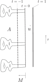
Figure 12. Mixed equation.

Using the moduli space of such pairs $(A,u)$ satisfying appropriate asymptotic boundary conditions, for $\tau\to\pm\infty$, we can define $HF(M;(L,b))$ the Floer homology with boundary condition $(L,b)$. (Here $b$ is a bounding cochain of $L$.) Note that we assume that $w_{2}(\mathcal{E}_{\Sigma})=[\Sigma]$. The basic analytic package to study such moduli spaces is established in [Lip, DFL1, DFL2].

Moreover using several Lagrangian submanifolds in place of a single $L$ in (mix4), we can extend $(L,b)\mapsto HF(M;(L,b))$ to a right filtered $A_{\infty}$ module over the filtered $A_{\infty}$ category $\mathfrak{Fukst}(R(\Sigma,\mathcal{E}_{\Sigma}))$.

Furthermore, the proof of Theorem 7.1 can be generalized in this gauge theoretical situation, and we can show that there is a bounding cochain $b_{M}$ of the immersed Lagrangian submanifold $R(K;\mathcal{E}_{M})$ such that $(R(M;\mathcal{E}_{M}),b_{M})$ via Yoneda embedding is sent to the right filtered $A_{\infty}$ module, $(L,b)\mapsto HF(M;(L,b))$.

Finally by a cobordism argument as in [Fu2, LL, DFL2] we can show

$$HF((R(M_{1};\mathcal{E}_{M_{1}}),b_{M_{1}}),(R(M_{2};\mathcal{E}_{M_{2}}),b_{M_{2}}))\cong I(M,\mathcal{E}_{M})$$ (7.10)

where $\partial M_{1}=\Sigma=-\partial M_{2}$ and $M$ is obtained from $M_{1}$ and $M_{2}$ by gluing them along $\Sigma$.

In the case when $R(M_{i};\mathcal{E}_{M_{i}})$ is an embedded Lagrangian submanifold for $i=1,2$, (7.10) is proved in [DFL2], where $b_{M_{i}}=0$. The general case is on the way being written.

The author emphasizes that the reference below is far from being complete. The references in the symplectic geometry are more emphasized than those in the complex or algebraic geometry.

References

- [Ab1] M. Abouzaid, Morse Homology, Tropical Geometry, and Homological Mirror Symmetry for Toric Varieties , Selecta Mathematica 15 (2009) 189–270.
- [Ab2] M. Abouzaid, A geometric criterion for generating the Fukaya category, Publ. Math. Inst. Hautes Études Sci. 112 (2010) 191–240.
- [Ab3] M. Abouzaid, Family Floer cohomology and mirror symmetry, Proceedings of the International Congress of Mathematicians-Seoul 2014. Vol. II, Kyung Moon Sa, Seoul (2014) 813–836.
- [Ab4] M. Abouzaid, The family Floer functor is faithful, J. European Math. Soc. 19 (2017) 2139–2217
- [Ab5] M. Abouzaid, Homological mirror symmetry without corrections, J. Amer. Math. Soc. 34 (2021) 1059–1173.
- [AB] M. Abouzaid and A. Blumberg, Arnold Conjecture and Morava K-theory, arXiv:2103.01507.
- [AAK] M. Abouzaid, D. Auroux and L. Katzarkov, Lagrangian fibrations on blowups of toric varieties and mirror symmetry for hypersurfaces, Publ. Math. Inst. Hautes Études Sci. 123 (2016) 199–282.
- [AFOOO] M. Abouzaid, K. Fukaya, Y.-G. Oh, H. Ohta and K. Ono, Quantum cohomology and split generation in Lagrangian Floer theory, in preparation.
- [ASe] M. Abouzaid and P. Seidel, An open string analogue of Viterbo functoriality Geometry and Topology 14 (2010), 627–718.
- [ASm] M. Abouzaid and I. Smith, Homological mirror symmetry for the 4-torus, Duke Math. J. 152 (2010) 373-440.
- [AJ] M. Akaho and D. Joyce, Immersed Lagrangian Floer theory, J. Differential Geometry 86 (2010) 381-500.
- [AM] S. Akbulut and J. McCarthy, Casson’s invariant for oriented homology 3-spheres- an exposition, Mathematical Notes, 36. Princeton University Press, Princeton, NJ, (1990).
- [Al] P. Albers, A Lagrangian Piunikhin-Salamon-Schwarz morphism and two comparison homomorphisms in Floer homology, Int. Math. Res. Not. IMRN 4 (2008).
- [At] M.F. Atiyah, New invariants of three and four dimensional manifolds, Proc. Symp. Pure Math. 48 (1988).
- [Au] D. Auroux, Mirror symmetry and T-duality in the complement of an anticanonical divisor, J. Gökova Geom. Topol. 1 (2007) 51–91.
- [AKO1] D. Auroux, L. Katzarkov and D. Orlov, Mirror symmetry for Del Pezzo surfaces: Vanishing cycles and coherent sheaves, Invent. Math. 166 (2006) 537–582.
- [AKO2] D. Auroux, L. Katzarkov and D. Orlov, Mirror symmetry for weighted projective planes and their noncommutative deformations, Ann. Math. 167 (2008) 867–943.
- [BX] Shaoyun Bai and Guangbo Xu, Arnold conjecture over integers, arXiv:2209.08599.
- [Be] A. Beilinson, Coherent sheaves on and problems in linear algebra, Funct. Anal. Appl. 12 (1978) 68–69.
- [BC] P. Biran and O. Cornea, Rigidity and uniruling for Lagrangian submanifolds, Geom. Topol. 13 (2009) 2881–2989.
- [BK] A. Bondal and M. Kapranov, Framed triangulated categories, Math. USSR. Sbornik 1 (1991 (1990 in Russian)) 93 - 107.
- [BW] N. Bottman and K. Wehrheim, Gromov compactness for squiggly strip shrinking in pseudoholomorphic quilts, Selecta Mathematica 24 (2018) pp 3381–3443.
- [BO] F. Bourgeois and A. Oancea, Symplectic homology, autonomous Hamiltonians, and Morse-Bott moduli spaces, Duke Math. J. 146 (2009) 71–174.
- [BD] P. Braam and S. Donaldson, Floer’s work on instanton homology, knots and surgery, The Floer Memorial Volume Birkhäuser, Basel (1995) 195-256.
- [CL] J. Cardy and D. Lewellen, Bulk and boundary operators in conformal field theory, Phys. Lett. B 259 (1991) 274–278.
- [CLL] Kw. Chan, S.-C. Lau, N. C. Leung, SYZ mirror symmetry for toric Calabi-Yau manifolds, J. Differential Geometry 90 (2012) 177–250.
- [Ch] C.-H. Cho, Non-displaceable Lagrangian submanifolds and Floer cohomology with non-unitary line bundle, J. Geom. Phys. 58 (2008), 1465–1476.
- [CO] C.-H. Cho and Y.-G. Oh, Floer cohomology and disc instantons of Lagrangian torus fibers in Fano toric manifolds, Asian J. Math. 10 (2006), 773–814.
- [CGRS] K. Cieliebak, A. Rita Gaio, I. Mundet i Riera and D. Salamon, The symplectic vortex equations and invariants of Hamiltonian group actions, J. Symplectic Geom. 1 (2002) 543–645.
- [CZ] C. Conley and E. Zehnder, The Birkhoff-Lewis fixed point theorem and a conjecture by V.I Arnold, Invent. Math. 73 (1983) 33–49.
- [DFL1] A. Daemi, K. Fukaya and M. Lipyanskiy, Lagrangians, SO(3)-instantons and Mixed Equation, arXiv:2109.07038.
- [DFL2] A. Daemi, K. Fukaya and M. Lipyanskiy, Lagrangians, SO(3)-instantons and Atiyah-Floer Conjecture, arXiv:2109.07032.
- [D1] S. Donaldson, An application of gauge theory to four-dimensional topology, J. Differential Geometry 18 (1983) 279–315.
- [D2] S. Donaldson, Irrationality and the h-cobordism conjecture, J. Differential Geometry 26 (1987) 141–168.
- [D3] S. Donaldson, Polynomial invariants for smooth four-manifolds, Topology 29 (1990) 257–315.
- [D4] S. Donaldson, Floer homology groups in Yang-Mills theory. With the assistance of M. Furuta and D. Kotschick. Cambridge Tracts in Mathematics, 147. Cambridge University Press, Cambridge, (2002) viii+236.
- [D5] S. Donaldson, Lefschetz pencils on symplectic manifolds, J. Differential Geometry 53, 205–236 (1999).
- [DS] S. Dostoglou and D.A. Salamon, Self-dual instantons and holomorphic curves, Ann. Math. 139 (1994) 581–640.
- [Dub] B. Dubrovin, Geometry of 2D topological field theories, Lecture note in Math. 1620 (1996), 120 - 348.
- [Dun] D. Duncan, Higher-rank instanton cohomology and the quilted Atiyah-Floer conjecture, arXiv:1311.5609.
- [Ei] D. Eisenbud, Homological algebra on a complete intersection, with an application to group representations , Trans. AMS. 260 (1980) 35–64.
- [EL] J. Evans and Y. Lekili, Generating the Fukaya categories of Hamiltonian G-manifolds. Journal of the American Mathematical Society 32 (2015) pp119–162.
- [FLTZ] B. Fang, C-C M. Liu, D. Traumann and E. Zaslow, T-duality and homological mirror symmetry for toric varieties, Advances in Math. 229 (2012) 1873–1911.
- [Fl1] A. Floer, Instanton invariant for 3-manifolds, Comm. Math. Phys. 118 (1988) 215–240.
- [Fl2] A. Floer, Morse theory for Lagrangian intersections, J. Differential Geometry28 (1988) 513–547.
- [Fl3] A. Floer, The unregularized gradient flow of the symplectic action, Comm. Pure Appl. Math. 41 (1988) 775–813.
- [Fl4] A. Floer, Symplectic fixed point and holomorphic sphere, Commun. Math. Phys. 120 (1989) 575–611.
- [Fl5] A. Floer, Cuplength estimates on Lagrangian intersections, Comm. Pure Appl. Math. 42 (1989) 335–356.
- [Fl6] A. Floer, Instanton Homology, Surgery and Knots, in “Geometry of Low-Dimensional Manifolds 1”, Ed. S.K. Donaldson and C.B. Thomas, LMS Lecture Note Series 150 (1990).
- [Fl7] A. Floer, Instanton homology and Dehn surgery, in Floer Memorial Volume, Hofer, Zender, and Taubes, Editors. Birkhäuser (1995) 77–98.
- [FH] A. Floer and H. Hofer, Symplectic homology. I. Open sets in , Math. Z. 215 (1994), 37–88.
- [Fu1] K. Fukaya, Morse homotopy, -Category, and Floer homologies, in “Proceedings of Garc Workshop on Geometry and Topology” ed. by H.J. Kim, Seoul National University (1994) 1-102.
- [Fu2] K. Fukaya, Floer homology for 3-manifolds with boundary -abstract -, in ‘Topology Geometry and Field theory’ ed by Fukaya, Furuta, Khono, Kotchick, World Scientific, Singapore (1994) 1-22.
- [Fu3] K. Fukaya, Floer homology of connected sum of homology 3-spheres, Topology 35 (1996) 88–136.
- [Fu4] K. Fukaya, Floer homology for 3-manifolds with boundary I (1997), never to be published but is available at http://www.math.kyoto-u.ac.jp/%7Efukaya/fukaya.html.
- [Fu5] K. Fukaya, Anti-self-dual equation on -manifolds with degenerate metric, Geom. Funct. Anal. 8 (1998) 466–528.
- [Fu6] K. Fukaya, Floer homology and mirror symmetry II, Minimal Surfaces, Geometric Analysis and Symplectic Geometry (Baltimore, MD, 1999), Adv. Stud. Pure Math. 34 (2002) 31–127.
- [Fu7] K. Fukaya, Floer homology for families-a progress report, Integrable systems, topology, and physics (Tokyo, 2000), Contemp. Math., 309, Amer. Math. Soc., Providence, RI, (2002) 33–68.
- [Fu8] K. Fukaya, Mirror symmetry of abelian varieties and multi-theta functions, J. Algebraic Geom. 11 (2002) 393–512.
- [Fu9] K. Fukaya, Galois symmetry on Floer cohomologies, Turkish J. Math. 27 (2003) 11–32.
- [Fu10] K. Fukaya, Multivalued Morse theory, Asymptotic Analysis, and Mirror symmetry, in ‘Graphs and patterns in mathematics and theoretical physics’, 205–278, Proc. Sympos. Pure Math., 73, Amer. Math. Soc., Providence, RI, (2005).
- [Fu11] K. Fukaya, Cyclic symmetry and adic convergence in Lagrangian Floer theory, Kyoto J. Math. 50 (2010) 521– 590.
- [Fu12] K. Fukaya, Categorification of invariants in gauge theory and sypmplectic geometry, Japanese Journal of Mathematics 13-1 (2018) 1–65, arXiv:1703.00603.
- [Fu13] K. Fukaya, Unobstructed immersed Lagrangian correspondence and filtered functor, arXiv:1706.02131.
- [FOOO1] K. Fukaya, Y.-G. Oh, H. Ohta and K. Ono, Lagrangian intersection Floer theory-anomaly and obstruction, Part I, AMS/IP Studies in Advaneced Math. 46.1, International Press/ Amer. Math. Soc. (2009). MR2553465.
- [FOOO2] K. Fukaya, Y.-G. Oh, H. Ohta and K. Ono, Lagrangian intersection Floer theory-anomaly and obstruction, Part II, AMS/IP Studies in Advanced Math. 46.2, International Press/ Amer. Math. Soc. (2009). MR2548482.
- [FOOO3] K. Fukaya, Y.-G. Oh, H. Ohta and K. Ono, Lagrangian Floer theory on compact toric manifolds I, Duke Math. J. 151 (2010), 23–174.
- [FOOO4] K. Fukaya, Y.-G. Oh, H. Ohta and K. Ono, Lagrangian Floer theory on compact toric manifolds II, - bulk deformation, Selecta Mathematica 17 (2011) 609–711.
- [FOOO5] K. Fukaya, Y.-G. Oh, H. Ohta and K. Ono, Anti-symplectic involution and Floer cohomology, Geometry and Topology 21 (2017) 1–106.
- [FOOO6] K. Fukaya, Y.-G. Oh, H. Ohta and K. Ono, Lagrangian Floer theory and mirror symmetry on compact toric manifolds, Astérisque 376, Société Mathématique de France (2016).
- [FOn] K. Fukaya and K. Ono, Arnold conjecture and Gromov-Witten invariant, Topology 38 (1999) 933–1048.
- [Ga] S. Ganatra, Symplectic cohomology and duality for the wrapped Fukaya category, Thesis, arXiv:1304.7312.
- [GPS1] S. Ganatra, J. Pardon and V. Shende, Covariantly functorial wrapped Floer theory on Liouville sectors, Publ. Math. Inst. Hautes Études Sci. 131 (2020) 73–200.
- [GPS2] S. Ganatra, J. Pardon and V. Shende, Sectorial descent for wrapped Fukaya categories, arXiv:1809.03427.
- [GPS3] S. Ganatra, J. Pardon and V. Shende, Microlocal Morse theory of wrapped Fukaya categories, arXiv:1809.08807.
- [Gi] A. Givental, Homological geometry I. Projective hypersurfaces, Selecta Mathematica 1 (1995) 325–345.
- [Go] W. Goldman, The symplectic nature of fundamental groups of surfaces. Adv. in Math. 54 (1984) 200–225.
- [GR] A. L. Gorodentsev, A. N. Rudakov, Exceptional vector bundles on projective spaces, Duke Math. J. 54 (1987) 115–130.
- [Gr] M. Gromov, Pseudoholomorphic curves in symplectic manifolds, Invent. Math. 82 (1985) 307–347.
- [GrS] M. Gross and B. Siebert, From real affine geometry to complex geometry, Ann. of Math. 174 (2011) 1301–1428.
- [GW] M. Gross and P. Wilson, Large Complex Structure Limits of K3 Surfaces, J. Differential Geometry 55 (2000) 475–546.
- [GS] V. Gugenheim and J. Stasheff, On perturbations and -structures, Festschrift in honor of G. Hirsch’s 60’th birthday, ed. L. Lemaire, Bull. Soc. Math. Belgique 38 (1986) 237–245.
- [Ha] R. Hartshone, Residue and duality, Lecture note in Math. 20 Springer (1966).
- [He] C. Herald, Legendrian cobordism and Chern-Simons theory on -manifolds with boundary, Comm. Anal. Geom. 2 (1994) 337–413.
- [HIV] K. Hori, A. Iqbal and C. Vafa, D-Branes and mirror symmetry, arXiv:hep-th/0005247.
- [HV] K. Hori and C. Vafa, Mirror symmetry, arXiv:hep-th/0002222.
- [HS] H. Hofer and D. Salamon, Floer homology and Novikov ring, Floer Memorial Volume Birkhäuser, Basel (1995) 483–524.
- [HW] K. Hori and J. Walcher, F-term equations near Gepner points, JHEP 0501 (2005) 008.
- [KL] A. Kapustin and A. Li, D-brane in Landau-Ginzburg models and algebraic geometry, JHEP 12 (2003) 005.
- [Ko1] M. Kontsevich, Homological algebra of Mirror symmetry, International congress of Mathematics, Birkhäuser, Zürich, 1995.
- [Ko2] M. Kontsevich, Lectures at ENS, Paris, Spring 1998, notes taken by J. Bellaiche, J.-F. Dat, I. Marin, G. Racinet and H. Randriambololona.
- [KS1] M. Kontsevich and Y. Soibelman, Homological mirror symmetry and torus fibrations, Symplectic geometry and mirror symmetry, World Scientific (2001) 203–263.
- [KS2] M. Kontsevich and Y. Soibelman, Affine structures and non-Archimedean analytic spaces, The unity of mathematics, Progr. Math., 244, Birkhäuser Boston, Boston, MA, (2006) 321–385.
- [KM] P. Kronheimer and T. Mrowka, Embedded surfaces and the structure of Donaldson’s polynomial invariants, J. Differential Geometry 41 (1995) 573–734.
- [LLW] R. Lee and W. Li, Floer homologies for Lagrangian intersections and instantons, arXiv:math/9506221.
- [LL] Y. Lekili and M. Lipyanskiy, Geometric composition in quilted Floer theory, Adv. Math. 236 (2013) 1–23.
- [LiY] Yang Li, Metric SYZ conjecture and non-archimedean geometry, arXiv:2007.01384.
- [Lie] W. Li, Floer homology for connected sums of homology 3-spheres, J. Differential Geom. 40 (1994) 129–154.
- [Lip] M. Lipyanskiy, Gromov-Uhlenbeck Compactness, arXiv:1409.1129.
- [LT] G. Liu and G. Tian, Floer homology and Arnold conjecture, J. Differential Geometry 49 (1998) 1–74.
- [MWo] C. Manolescu and C. Woodward, Floer homology on the extended moduli space, Perspective in analysis, geometry, and topology, 283–329, Progre. Math. 296, Birkhäuser, New York.
- [MWe] J. Marsden and A. Weinstein, Reduction of symplectic manifolds with symmetry, Reports on Mathematical Physics 5 (1974) 121–130.
- [MWW] S. Ma’u, K. Wehrheim and C. Woodward, -functor for Lagrangian correspondences, Selecta Math. 24 (2018) 1913–2002.
- [McSa] D. McDuff and D. Salamon, -Holomorphic Curves and Quantum Cohomology, Amer. Math. Soc., Providence, RI, University Lecture Seires 6 (1994)
- [NNU1] T. Nishinou, Y. Nohara and K.Ueda, Toric degenerations of Gelfand-Cetlin systems and potential functions, Adv. Math. 224 (2010) 648–706.
- [NNU2] T. Nishinou, Y. Nohara and K.Ueda, Potential functions via toric degenerations, Proc. Japan Acad. Ser. A Math. Sci. 88 (2012), 31–33.
- [Nov] S. Novikov, Multivalued functions and functional - an analogue of Morse theory, Sov. Math. Dokl. 24 (1981) 222–225.
- [Oh] Y.-G. Oh, Floer cohomology of Lagrangian intersections and pseudo-holomorphic disks I, II, Comm. Pure and Appl. Math. 46 (1993) 949–994, 995–1012; Addenda, ibid, 48 (1995) 1299 –1302.
- [On] K. Ono, On the Arnold conjecture for weakly monotone symplectic manifolds, Invent. Math. 119 (1995) 519–537.
- [Or] D. Orlov, Triangulated categories of singularities and D-branes in Landau-Ginzburg models , Math. Inst. Seklova 246 (2004) 227–249.
- [PZ] A. Polishchuk and E. Zaslow, Categorical Mirror Symmetry: The Elliptic Curve, Adv. Theor. Math. Phys. 2 (1998) 443–470.
- [Ra] P. Rabinowitz, Periodic solutions of a Hamiltonian system on a prescribed energy surface, J. Differential Equations 33 (1979) 336–352.
- [Ru1] Y. Ruan, Topological sigma model and Donaldson-type invariants in Gromov theory, Duke Math. J. 83 (1996) 461–500.
- [Ru2] Y. Ruan, Virtual neighborhood and pseudo-holomorphic curve, Turkish J. Math. 23 (1999) 161–231.
- [RT1] Y. Ruan and G. Tian, A mathematical theory of quantum cohomology, J. Differential Geom. 42 (1995) 259–367.
- [RT2] Y. Ruan and G. Tian, Higher genus symplectic invariants and sigma models coupled with gravity, Invent. Math. 130 (1997) 455–516.
- [Sa] K. Saito, Period mapping associated to a primitive form, Publ. R.I.M.S. 19 (1983), 1231 - 1261.
- [SW] D. Salamon and K. Wehrheim, Instanton Floer homology with Lagrangian boundary conditions, Geometry and Topology 12 (2008) 747–918.
- [Se1] P. Seidel, Graded Lagrangian submanifolds, Bull. Soc. Math. France 128 (2000) 103–146.
- [Se2] P. Seidel, More about vanishing cycles and mutation, Symplectic geometry and mirror symmetry (Seoul, 2000), (2001) 429–465
- [Se3] P. Seidel, A long exact sequence for symplectic Floer cohomology, Topology 42 (2003) 1003–1063.
- [Se4] P. Seidel, Fukaya categories and Picard-Lefschetz theory, ETH Lecture Notes Series 8, European Math. Soc., (2008).
- [Se5] P. Seidel, Homological mirror symmetry for the quartic surface, Memoirs of the Amer. Math. Soc., 1116 (2015).
- [She1] N. Sheridan, Homological Mirror Symmetry for Calabi-Yau hypersurfaces in projective space, Invent. Math. 199 (2015) 1–186.
- [She2] N. Sheridan, On the Fukaya category of a Fano hypersurface in projective space, Publ. Math. Inst. Hautes Études Sci. 124 (2016) 165–317.
- [Shk] D. Shklyarov, Matrix factorization and higher residue pairing, Adv. in Math. 292 (2016) 181-209.
- [So] J. Solomon, Involutions, obstructions and mirror symmetry, Adv. Math. 367 (2020) 107107, 1–52.
- [St] J. Stasheff, Homotopy associativity of H-spaces I, II, Trans. Amer. Math. Soc. 108 (1963) 275–312.
- [SYZ] A. Strominger, S.-T. Yau and E. Zaslow, Mirror Symmetry is T-Duality, Nucl.Phys. B479 (1996) 243–259.
- [Ta] C. Taubes, Casson’s invariant and gauge theory, J. Differential Geometry 31 (1990) 547–599.
- [Tu] J. Tu, On the reconstruction problem in mirror symmetry, Adv. Math. 256 (2014) 449–478.
- [Ue] K. Ueda, Homological Mirror Symmetry for Toric del Pezzo Surfaces, Communications in Mathematical Physics 264 (2006) 71–85.
- [Va] C. Vafa, Topological mirrors and quantum rings, Mirror symmetry I, AMS/IP Stud. Adv. Math. 9 (1998) 97–120.
- [Weh] K. Wehrheim, Lagrangian boundary conditions for anti-self-dual instantons and the Atiyah-Floer conjecture, Conference on Symplectic Topology. J. Symplectic Geom. 3 (2005) 703–747.
- [We] A. Weinstein, The symplectic “category” , in Differential Geometric methods in mathematical Physics (Clausthal, 1980) Lecture notes in Math., 905 45–51, Springer, Berlin.
- [Wi1] E. Witten, Supersymmetry and Morse theory, J. Differential Geom. 17 (1982) 661-692.
- [Wi2] E. Witten, Topological quantum field theory. Comm. Math. Phys. 117 (1988) 353–386.
- [Wi3] E. Witten, Topological sigma model, Comm. Math. Phys. 118 (1988) 411-449.
- [Wi4] E. Witten, Phases of N = 2 theories in two dimensions, Nucl. Phys. B 403 (1993) 159–222.
- [Wi5] E. Witten, Monopoles and four-manifolds, Math. Res. Lett. 1 (1994) 769–796.
- [WW1] K. Wehrheim and C. Woodward, Quilted Floer cohomology, Geometry and Topology 14 (2010) 833–902.
- [WW2] K. Wehrheim and C. Woodward, Functoriality for Lagrangian correspondences in Floer theory, Quantum Topology 1 (2010) 129–170.
- [WW3] K. Wehrheim and C. Woodward, Floer cohomology and geometric composition of Lagrangian correspondences, Advances in Mathematics 230 (2012) 177–228.
- [WW4] K. Wehrheim and C. Woodward, Pseudoholomorphic quilts, Journal of Symplectic Geometry 13 (2015) 849-904.
- [Wo] C. Woodward, Quantum Kirwan morphism and Gromov-Witten invariants of quotients I, II, III, Transformation Groups 20 (2015) 507–556, 881–920, 1155–1193.
- [WX] C. Woodward and G. Xu, An open quantum Kirwan map, arXiv:1806.06717.
- [Yo] T. Yoshida, Floer homology and holomorphic curves - Atiyah conjecture, preprint, 1992.
- [Yu] H. Yuan, Family Floer program and non-archimedean SYZ mirror construction, arXiv:2003.06106.