claimClaim remarkRemark hypothesisHypothesis

Yuexin Zhou, Chao Ding, and Yangjing Zhang







Strong variational sufficiency of nonsmooth optimization problems on Riemannian manifolds


Yuexin Zhou
Institute of Applied Mathematics, Academy of Mathematics and Systems Science, Chinese Academy of Sciences, Beijing, P.R. China, School of Mathematical Sciences, University of Chinese Academy of Science, Beijing, P.R. China.
().
zhouyuexin19@mails.ucas.ac.cn

  
Chao Ding
Institute of Applied Mathematics, Academy of Mathematics and Systems Science, Chinese Academy of Sciences, Beijing, P.R. China, School of Mathematical Sciences, University of Chinese Academy of Science, Beijing, P.R. China.
().
dingchao@amss.ac.cn

  
Yangjing Zhang
Institute of Applied Mathematics, Academy of Mathematics and Systems Science, Chinese Academy of Sciences, Beijing, P.R. China.
().
yangjing.zhang@amss.ac.cn




Abstract
The Riemannian Augmented Lagrangian Method (RALM), a recently proposed algorithm for nonsmooth optimization problems on Riemannian manifolds, has consistently exhibited high efficiency as evidenced in prior studies [42, 43]. It often demonstrates a rapid local linear convergence rate. However, a comprehensive local convergence analysis of the RALM under more realistic assumptions, notably without the imposition of the uniqueness assumption on the multiplier, remains an uncharted territory. In this paper, we introduce the manifold variational sufficient condition and demonstrate that its strong version is equivalent to the manifold strong second-order sufficient condition (M-SSOSC) in certain circumstances. Critically, we construct a local dual problem based on this condition and implement the Euclidean proximal point algorithm, which leads to the establishment of the linear convergence rate of the RALM. Moreover, we illustrate that under suitable assumptions, the M-SSOSC is equivalent to the nonsingularity of the generalized Hessian of the augmented Lagrangian function, which is an essential attribute for the semismooth Newton-type methods.


keywords: 
nonsmooth optimizations on Riemannian manifold, strong variational sufficiency, augmented Lagrangian method, rate of convergence

 
90C30, 90C46, 49J52, 65K05





1 Introduction


This paper is concerned with the nonsmooth optimization problems on Riemannian manifolds in the following form:



(1)

$$\begin{array}[]{ll}\min&f(x)+\theta(g(x))\\
\text{ s.t. }&x\in\mathcal{M},\end{array}$$



where $\mathcal{M}$ is a connected Riemannian manifold, $f:\mathcal{M}\rightarrow\mathbb{R}$ and $g:\mathcal{M}\rightarrow\mathbb{Y}$ are continuously differentiable functions, $\mathbb{Y}$ is a Euclidean space equipped with a scalar
product $\langle\cdot,\cdot\rangle$ and its induced
norm $\|\cdot\|$, $\theta:\mathbb{Y}\rightarrow(-\infty,\infty]$ is a proper closed convex function. If $\theta$ is an indicator function of a closed convex set, then (1) is a constrained manifold optimization problem. Applications of (1) arise in various scenarios such as principal component analysis problems [44], low-rank matrix completion problems [7], orthogonal dictionary learning problems [38, 12] and compressed modes problems [29]. One may refer to [1, 20] for more details.


Different algorithms have been designed for solving the manifold nonsmooth optimization problem (1), such as subgradient methods [14, 16], proximal gradient methods [9, 21, 22], alternating direction methods of multipliers [24, 25] and proximal point methods (PPA) [8, 15]. In recent papers [13, 42], the augmented Lagrangian method (ALM) has also been extended to solve the nonsmooth manifold optimization problem (1). By adding a perturbation parameter $u$, we can obtain the perturbed problem for (1):



(2)

$$\begin{array}[]{ll}\min&\varphi(x,u):=f(x)+\theta(g(x)+u)\\
\text{ s.t. }&x\in\mathcal{M}.\end{array}$$



Problem (2) is reduced to problem (1) when $u=0$.
The Lagrangian function for (1) is




$$l(x,y)=\inf_{u}\{\varphi(x,u)-\left\langle y,u\right\rangle\}=L(x,y)-\theta^{*}(y),$$



where $L(x,y)=f(x)+\left\langle y,g(x)\right\rangle$ and $\theta^{*}$ is the conjugate function of $\theta$. Moreover, for $\rho>0$, the augmented Lagrangian function for (1) is defined by



(3)

$$l^{\rho}(x,y)=\inf_{u}\big{\{}\varphi(x,u)-\left\langle y,u\right\rangle+\frac{\rho}{2}\|u\|^{2}\big{\}}.$$



The inexact Riemannian augmented Lagrangian method (RALM) proposed in [13, 42] for solving (1) then takes the form of



(4)

$$\left\{\begin{array}[]{l}\displaystyle x^{k+1}\approx\bar{x}^{k+1}:=\underset{x\in\mathcal{U}}{\operatorname{argmin}}\;l^{\rho_{k}}\left(x,y^{k}\right),\\
\displaystyle y^{k+1}=y^{k}+\tilde{\rho}_{k}\nabla_{y}l^{\rho_{k}}\left(x^{k+1},y^{k}\right),\end{array}\right.$$



where $\mathcal{U}$ is a subset of $\mathcal{M}$, $\tilde{\rho}_{k}>0$ and $\rho_{k}>0$ are nondecreasing sequences satisfying $\tilde{\rho}_{k}\leq\rho_{k}$. As evidenced in [42, 43], the RALM consistently displays high efficiency, often demonstrating a fast local linear convergence rate. Furthermore, when the semismooth Newton method is utilized to solve the augmented Lagrangian subproblems in (4), it has frequently been observed that for certain problem classes, the associated generalized Hessian of the augmented Lagrangian function remains consistently positive definite. Nevertheless, the fast local convergence rate the algorithm under more realistic assumptions (specifically, without imposing the singletonness assumption on the multiplier) and the characterization of the non-singularity of the generalized Hessian of the augmented Lagrangian function have yet to be fully explored.


The classical Euclidean ALM, originally proposed by Hestenes [17] and Powell [30] for equality constrained problems, was later expanded to nonlinear programming (NLP) by Rockafellar [32]. Over the decades, the convergence analysis of ALM under the Euclidean setting has been extensively studied. In literature, it is posited that the local linear convergence rate of ALM for NLP requires both the linear independence constraint qualification (LICQ) and the second-order sufficient condition (SOSC) (see e.g., [5, 10, 28]). For non-convex non-polyhedral problems, such as nonlinear second-order cone programs and semidefinite programs, Liu and Zhang [27] and Sun et al. [39] obtain the local linear convergence rate of ALM under the constraint non-degeneracy condition and the strong SOSC at Karush-Kuhn-Tucker (KKT) points, respectively. More recently, for $\mathcal{C}^{2}$-cone reducible constraints, Kanzow and Steck [23] obtained the primal-dual linear convergence rate under the strong Robinson constraint qualification (SRCQ) and SOSC. These analyses for the Euclidean ALM all hinge on the uniqueness of the multipliers. Turning to the RALM, the first convergence result is established in [42] under the constant positive linear dependence constraint qualification and LICQ. Subsequently, the local linear convergence rate for the RALM was provided in [43] under the manifold strict Robinson constraint qualification (M-SRCQ) and the manifold second-order sufficient condition (M-SOSC). Nevertheless, existing convergence results for the RALM still necessitate a unique multiplier. Interestingly, we have observed that the RALM can still perform effectively in certain scenarios even when the multiplier set is not a singleton. This observation has driven us to explore alternative conditions that could ensure the local linear convergence rate of the RALM without requiring the uniqueness of the multipliers.


The recent studies [36, 41] shed light on the possibility of relaxing the uniqueness assumption of the multipliers under the so-called (strong) variational sufficient condition. In [35], Rockafellar introduces the concept of variational (strong) convexity, which requires the function value and the subdifferential of the non-convex function to be locally identical to a (strongly) convex function. By utilizing this property, the (strong) variational sufficient condition for optimizations in Euclidean setting is built up by requiring the perturbed augmented objective function to be variationally (strongly) convex with respect to a first-order stationary point. It is proven in [35] that the strong variational sufficient condition implies the local strong convexity of the augmented Lagrangian function and the augmented tilt stability. Furthermore, it is demonstrated that strong variational sufficiency is equivalent to the strong SOSC
if the function $\theta$ in (1) (when the manifold $\mathcal{M}$ is taken as a Euclidean space) is a polyhedral function ([35]) or an indicator function of a second-order cone or semidefinite cone ([41]). By leveraging the strong convexity of the augmented Lagrangian function, one may be able to construct an augmented dual problem locally around a KKT pair and apply the PPA to this dual problem to achieve a local linear rate. Rockafellar [36] then extends the classical results in [33], which posit the equivalence of the dual PPA and primal ALM for convex problems, to obtain the local linear convergence rate of ALM under the strong variational sufficient condition. Inspired by this approach, our objective is to extend the (strong) variational sufficient condition to manifold optimization. The first challenge here is defining convexity on a manifold. It is widely understood that translating the concept of convexity from Euclidean settings to functions and sets on a Riemannian manifold is not straightforward, primarily because a standard ‘line segment’ connecting two points $x$ and $y$ on a manifold cannot be represented by a convex combination of $x$ and $y$. To address this issue, we propose an alternative problem that is locally equivalent to (1). Suppose that $(\bar{x},\bar{y})$ is a stationary point of problem (2), as defined in (11). Let $R_{\bar{x}}$ denote the retraction and $T_{\bar{x}}\mathcal{M}$ denote the tangent space of $\mathcal{M}$ at $\bar{x}$ (see Section 2 for definitions). We locally transform the manifold problem (1) into an optimization problem on the tangent space $T_{\bar{x}}\mathcal{M}$ at $\bar{x}$ as follows:



(5)

$$\begin{array}[]{ll}\min&f\circ R_{\bar{x}}(\xi)+\theta(g\circ R_{\bar{x}}(\xi))\\
\text{ s.t. }&\xi\in T_{\bar{x}}\mathcal{M}.\end{array}$$



This problem is locally equivalent to (1) if we set $x=R_{\bar{x}}(\xi)$. Compared with (1), problem (5) is more approachable due to $T_{\bar{x}}\mathcal{M}$ being a Euclidean space.
Consequently, we can now explore properties related to the convexity of (5).


In this paper, we establish the ALM for solving (5), which is locally equivalent to RALM (4) for solving (1). By assuming the variational sufficient condition for problem (5) (a property we will refer to as the manifold variational sufficient condition), we are able to construct a local augmented dual problem in Euclidean space for (1).
Furthermore, we discover that the manifold strong variational sufficient condition is equivalent to the manifold strong second-order sufficient condition (M-SSOSC) under certain circumstances. This also implies that the manifold strong variational sufficient condition is independent of the choice of retractions. Consequently, by applying PPA to the local dual problem, we ultimately obtain R-linear convergence rate of the primal iterations of RALM and Q-linear rate of the multipliers sequence. Moreover, we show that the M-SSOSC is also equivalent to the non-singularity of the generalized Hessian of the augmented Lagrangian function, which ensures the efficiency of the semismooth Newton method when solving the subproblem of RALM.


The rest of the paper is organized as follows. In Section 2, we revisit some fundamentals of smooth manifolds and nonsmooth analysis. In Section 3, we define the local equivalent problem for (1) in the tangent space and explore the relation of Lagrangian functions and first-order conditions between these two problems. The variational sufficient condition is discussed in Section 4. Moreover, the local duality under variational sufficient condition is given in this section. Section 5 establishes the local convergence analysis of RALM. The semismooth Newton method for solving RALM subproblem and its local convergence rate are discussed in Section 6. The applications and numerical results are presented in Section 7. Finally, we give our conclusion in Section 8.



2 Preliminaries and notations


We begin by introducing some basic concepts of manifolds that will be used in our discussion. Most of the properties referred to below can be found in the literature, specifically in [2, 26].


Let $\mathcal{M}$ be an $n$-dimensional smooth manifold and $x\in\mathcal{M}$. $\mathfrak{F}_{x}(\mathcal{M})$ is defined as the set of all smooth real-valued functions on a neighborhood of $x$. The mapping $\xi_{x}$ from $\mathfrak{F}_{x}(\mathcal{M})$ to $\mathbb{R}$ such that there exists a curve $\gamma$ on $\mathcal{M}$ with $\gamma(0)=x$ satisfying $\xi_{x}f:=\dot{\gamma}(0)f:=\left.\dfrac{d(f(\gamma(t)))}{dt}\right|_{t=0}$ for all $f\in\mathfrak{F}_{x}(\mathcal{M})$ is called a tangent vector, and the tangent space $T_{x}\mathcal{M}$ is the set of all tangent vectors to $\mathcal{M}$ at $x$. If $\mathcal{M}$ is embedded in a Euclidean space $\mathbb{X}$, the normal space $N_{x}\mathcal{M}$ is defined as the orthogonal complement of $T_{x}\mathcal{M}$ in $\mathbb{X}$. The tangent bundle is defined as $T\mathcal{M}:=\bigcup_{x}T_{x}\mathcal{M}$, which is the set of all tangent vectors to $\mathcal{M}$. A map $V:\mathcal{M}\rightarrow T\mathcal{M}$ is called a vector field on $\mathcal{M}$ if $V(x)\in T_{x}\mathcal{M}$ for all $x\in\mathcal{M}$.


Let $F:\mathcal{M}\rightarrow\mathbb{X}$ be a smooth mapping. The mapping $DF(x):T_{x}\mathcal{M}\rightarrow T_{F(x)}\mathbb{X}$ which is defined by $\left(DF(x)\xi_{x}\right)f:=\xi_{x}(f\circ F)$ for $\xi_{x}\in T_{x}\mathcal{M}$ and $f\in\mathfrak{F}_{F(x)}(\mathbb{X})$, is a linear mapping called the differential of $F$ at $x$. If $\mathcal{M}$ is embedded in a Euclidean space, then $DF(x)$ is reduced to the classical definition of directional derivative, i.e., $\displaystyle DF(x)\xi_{x}=\lim_{t\rightarrow 0}\frac{F\left(x+t\xi_{x}\right)-F(x)}{t}$. To distinguish it from the Riemannian differential, we use $h^{\prime}(x)\xi$ to represent the traditional directional derivative in the direction $\xi$ and $\nabla h(x)$ to be the Euclidean gradient of $h$.


Riemannian metric $\langle\cdot,\cdot\rangle_{x}$ is a smoothly varying inner product with respect to $x$ defined for tangent vectors. A differentiable manifold whose tangent spaces are endowed with Riemannian metrics is called a Riemannian manifold. When no confusions arise, we will use $\langle\cdot,\cdot\rangle$ instead of $\langle\cdot,\cdot\rangle_{x}$ for simplicity. The induced norm of this inner product is denoted by $\|\cdot\|$ with the subscript being omitted. Given $f\in\mathfrak{F}_{x}(\mathcal{M})$, the gradient of $f$ at $x$, denoted by $\operatorname{grad}f(x)$, is defined as the unique tangent vector that satisfying $\langle\operatorname{grad}f(x),\xi\rangle:=\xi_{x}f$ for all $\xi\in T_{x}\mathcal{M}$.


The length of a curve $\gamma:[a,b]\rightarrow\mathcal{M}$ on a Riemannian manifold is defined by
$L(\gamma)=\int_{a}^{b}\sqrt{\langle\dot{\gamma}(t),\dot{\gamma}(t)\rangle}\mathrm{d}t$, and the Riemannian distance on $\mathcal{M}$ is given by $d(y,z):=\inf_{\gamma\in\Gamma}L(\gamma)$, where $\Gamma$ represents the set of all curves in $\mathcal{M}$ joining points $y$ and $z$. Then the set $\{y\in\mathcal{M}\mid d(x,y)<\delta\}$ is a neighborhood of $x$ with radius $\delta>0$. A geodesic is a curve on $\mathcal{M}$ which locally minimizes the arc length. For every $\xi\in T_{x}\mathcal{M}$, there exists an interval $\mathcal{I}$ containing zero and a unique geodesic $\gamma(\cdot;x,\xi):\mathcal{I}\rightarrow\mathcal{M}$ such that $\gamma(0)=x$ and $\dot{\gamma}(0)=\xi$. The mapping
$\operatorname{Exp}_{x}:T_{x}\mathcal{M}\rightarrow\mathcal{M}$, $\xi\mapsto\operatorname{Exp}_{x}(\xi)=\gamma(1;x,\xi)$
is called the exponential mapping on $x\in\mathcal{M}$. A vector field $X$ is parallel along a smooth curve $\gamma$ if $\nabla_{\dot{\gamma}}X=0$. where $\nabla$ is the Riemannian connection on $\mathcal{M}$.
Given a smooth curve $\gamma$ and $\eta\in T_{\dot{\gamma}(0)}\mathcal{M}$, there exists a unique parallel vector field $X_{\eta}$ along $\gamma$ such that $X_{\eta}(0)=\eta$. We define the parallel transport along $\gamma$ to be $P_{\gamma}^{0\rightarrow t}\eta:=X_{\eta}(t)$. When the geodesic from $p$ to $q$ is unique, denoted by $\gamma_{pq}$, we define $P_{pq}:=P_{\gamma_{pq}}^{0\rightarrow 1}$.


A retraction on a manifold $\mathcal{M}$ is a smooth mapping $R$ from the tangent bundle $T\mathcal{M}$ onto $\mathcal{M}$ satisfying $R_{x}\left(0_{x}\right)=x$ and $DR_{x}\left(0_{x}\right)=\mathrm{id}_{T_{x}\mathcal{M}}$. Let $R_{x}$ denote the restriction of $R$ to $T_{x}\mathcal{M}$. The Riemannian Hessian of $f\in\mathfrak{F}_{x}(\mathcal{M})$ at a point $x$ in $\mathcal{M}$ is defined as the (symmetric) linear mapping $\operatorname{Hess}f(x)$ from $T_{x}\mathcal{M}$ into itself satisfying $\operatorname{Hess}f(x)\xi=\nabla_{\xi}\operatorname{grad}f(x)$ for all $\xi\in T_{x}\mathcal{M}$. By [2, Proposition 5.5.6], if $\operatorname{grad}f(x)=0$, then



(6)

$$\operatorname{Hess}f(x)=\operatorname{Hess}\left(f\circ R_{x}\right)\left(0_{x}\right).$$





Suppose that a subset $\mathcal{A}\subset\mathcal{M}$. The epigraph of a function $F:\mathcal{A}\rightarrow(-\infty,\infty]$ is defined as $\operatorname{epi}F:=\{(x,\alpha)\in\mathcal{A}\times\mathbb{R}\mid F(x)\leq\alpha\}$. A proper function $F:\mathcal{A}\rightarrow(-\infty,\infty]$ is called lower semi-continuous (lsc) if $\operatorname{epi}F$ is closed. When considering the manifold $\mathcal{M}$ as a topology space, we can use the classical definition of lower semicontinuity of a function $F:\mathcal{M}\to(-\infty,\infty]$, that for any $x\in\mathcal{M}$, it holds that $\liminf_{y\rightarrow x}f(y)\geq f(x)$. It is not difficult to verify that this definition is equivalent to the epigraph definition if we consider $\mathcal{M}$ itself as a closed set of the topology space. The following definition of the Fréchet subdifferential is taken from [4, Corollary 4.5].



Definition 2.1.


Let $f:\mathcal{M}\rightarrow\mathbb{R}$ be a function defined on a Riemannian manifold, and $(\mathcal{U},\varphi)$ is a chart of $\mathcal{M}$. The Fréchet subdifferential $\partial f(x)$ of $f$ at a point $x\in\operatorname{dom}f=\{x\in M:f(x)<\infty\}$ is defined as




$$\partial f(x)
=\big{\{}D\varphi(x)\zeta\mid\zeta\in\mathbb{R}^{n},\liminf_{v\rightarrow 0}\frac{f\circ\varphi^{-1}(\varphi(x)+v)-f(x)-\langle\zeta,v\rangle}{\|v\|}\geq 0\big{\}}$$






$$=\big{\{}D\varphi(x)\zeta\mid\zeta\in\partial\left(f\circ\varphi^{-1}\right)(\varphi(x))\big{\}}.$$







From this definition, one may deduce that $\partial f(x)=\partial\left(f\circ R_{x}\right)\left(0_{x}\right)$ for any given retraction $R$.


With the distance function $d(\cdot,\cdot)$ defined above, the Lipschitz property of functions can be extended to manifold. A function $f:\mathcal{M}\to\mathbb{R}$ is Lipschitz of rank $L>0$ in a set $\mathcal{U}$ if for any $y,z\in\mathcal{U}$, $|f(y)-f(z)|\leq Ld(y,z)$. If there exists a neighborhood $\mathcal{U}$ of $x\in\mathcal{M}$ such that $f$ is Lipschitz of rank $L$ on $\mathcal{U}$, we say that $f$ is Lipschitz of rank $L$ at $x$; if for every $x\in\mathcal{M}$, $f$ is Lipschitz of rank $L$ at $x$ for some $L>0$, then $f$ is said to be locally Lipschitz on $\mathcal{M}$. The generalized directional derivative of a locally Lipschitz function $f$ at $x\in\mathcal{M}$ in the direction $v\in T_{x}\mathcal{M}$, is defined in [18] as




$$f^{\circ}(x;v):=\limsup_{y\rightarrow x,t\downarrow 0}\dfrac{f\circ\varphi^{-1}(\varphi(y)+tD\varphi(x)v)-f\circ\varphi^{-1}(\varphi(y))}{t},$$



where $(\mathcal{U},\varphi)$ is a chart containing $x$. The definition of the generalized directional derivative implies that $f^{\circ}(x,v)=\left(f\circ R_{x}\right)^{\circ}(0_{x},v)$ for any retraction.
The Clarke subdifferential of a locally Lipschitz function $f$ at $x\in\mathcal{M}$, denoted by $\partial_{C}f(x)$, is defined as




$$\partial_{C}f(x)=\left\{\xi\in T_{x}\mathcal{M}\mid\langle\xi,v\rangle\leq f^{\circ}(x;v)\text{ for all }v\in T_{x}\mathcal{M}\right\}.$$



According to [18, Proposition 2.5], an equivalence can be established between the Clarke subdifferential of $f$ and the Clarke subdifferential of $f\circ R$ for any retraction $R$, as described below.



Proposition 2.2.


Let $\mathcal{M}$ be a Riemannian manifold and $x\in\mathcal{M}$. Suppose that $f:\mathcal{M}\to\mathbb{R}$ is Lipschitz near $x$ and $(\mathcal{U},\varphi)$ is a chart at $x$. Then




$$\partial_{C}f(x)=D\varphi(x)\left[\partial_{C}\left(f\circ\varphi^{-1}\right)(\varphi(x))\right].$$



Therefore, we have $\partial_{C}f(x)=\partial_{C}\left(f\circ R_{x}\right)\left(0_{x}\right)$ for any retraction $R_{x}$.




As mentioned in the introduction, a useful tool for analyzing the local convergence of ALM is the variational sufficient condition. We first introduce the variational convexity proposed in [35].



Definition 2.3.


Given a lsc function $F:\mathbb{R}^{n}\rightarrow(-\infty,\infty]$, the variational convexity of $F$ with respect to a pair $(\bar{w},\bar{z})\in\operatorname{gph}\partial F$ is said to hold if there exist open convex neighborhoods $\mathcal{W}$ of $\bar{w}$ and $\mathcal{Z}$ of $\bar{z}$ such that
there exists a proper lsc convex function $h\leq F$ on $\mathcal{W}$ such that




$$[\mathcal{W}\times\mathcal{Z}]\cap\operatorname{gph}\partial h=[\mathcal{W}\times\mathcal{Z}]\cap\operatorname{gph}\partial F$$



and, for $(w,z)$ belonging to this common set, $h(w)=F(w)$. If $h$ is strongly convex on $\mathcal{W}$, we say that $F$ is variationally strongly convex with respect to $(\bar{w},\bar{z})$.




For a Euclidean optimization problem,
the variational sufficient condition is said to hold at a first-order stationary point if the augmented perturbed objective function $\varphi^{\rho}$ is variationally convex, with $\varphi^{\rho}(x,u)=\varphi(x,u)+\frac{\rho}{2}\|u\|^{2}$. The strong variational sufficient condition holds if $\varphi^{\rho}$ is variationally strongly convex.



3 The localization problems and the Lagrangian functions


At a given point $x\in\mathcal{M}$, the optimization problem (1) can be locally transformed into an equivalent optimization problem on the tangent space $T_{x}\mathcal{M}$ at $x$ by employing the retraction $R_{x}:T_{x}\mathcal{M}\to\mathcal{M}$. This is made possible by the inverse function theorem [26, Theorem 4.5], which establishes that any retraction is a diffeomorphism within a neighborhood of $0_{x}$ in the tangent space $T_{x}\mathcal{M}$ for a general Riemannian manifold. The following definition given in [19] defines the injectivity radius of a Riemannian manifold with respect to retraction, which aligns with the classical definition of injectivity radius [6, Definition 10.19], when the retraction is chosen as the exponential mapping.



Definition 3.1.


The injectivity radius of manifold $\mathcal{M}$ at a point $x$ with respect to retraction $R_{x}$, denoted by $r_{R_{x}}$, is the supremum over radii $r>0$ such that $R_{x}$ is defined and is a diffeomorphism on the open ball $B_{x}(r)=\left\{v\in\mathrm{T}_{x}\mathcal{M}:\|v\|<r\right\}$. By the inverse function theorem, $r_{R_{x}}>0$.




Additionally, as outlined in [6, Proposition 10.22], we have $d(x,y)=\|v\|$ within the ball $B_{x}(r_{\operatorname{Exp}_{x}})$ if $y=\operatorname{Exp}_{x}(v)$.


To construct a problem that is locally equivalent to (1), we begin by introducing the following function defined on the tangent space at a given point $x\in\mathcal{M}$. Definition 3.2 on tangent space is different from the pullback function defined in [2, Section 4], where the latter is formulated as $f\circ R$ at each point on the manifold.



Definition 3.2.


Let $x\in\mathcal{M}$ and $r_{R_{x}}$ be the injectivity radius of $\mathcal{M}$ at $x$ with respect to $R_{x}$. For a given function $F:\mathcal{M}\to\mathbb{R}$, we define $F_{R_{x}}:T_{x}\mathcal{M}\to(-\infty,\infty]$ by



(7)

$$F_{R_{x}}(\xi)=\left\{\begin{array}[]{cl}F\left(R_{x}\xi\right),&\xi\in B_{x}(r_{R_{x}}),\\
+\infty,&\xi\notin B_{x}(r_{R_{x}}).\end{array}\right.$$







It is worth noting that the lower semicontinuity of $F$ is inherited by $F_{R_{x}}$ within the ball $B_{x}(r_{R_{x}})$. However, this continuity may not hold on its boundary. Fortunately, this limitation does not affect our discussions since our focus is solely on the properties of $F_{R_{x}}$ within the ball $B_{x}(r_{R_{x}})$.


For a given point $\bar{x}$ and a retraction $R_{\bar{x}}$, applying (7) to $f$ and $g$, we obtain the following problem on tangent space $T_{\bar{x}}\mathcal{M}$ as



(8)

$$\begin{array}[]{ll}\min&f_{R_{\bar{x}}}(\xi)+\theta(g_{R_{\bar{x}}}(\xi))\\
\text{ s.t. }&\xi\in T_{\bar{x}}\mathcal{M},\end{array}$$



where $f_{R_{\bar{x}}}$ and $g_{R_{\bar{x}}}$ are defined by (7). By Definitions 3.1 and 3.2, problem (8) is locally equivalent to problem (1) in the injectivity ball $B_{\bar{x}}(r_{R_{\bar{x}}})$ as we can build the one-to-one relationship $x=R_{\bar{x}}(\xi)$ for any $\xi\in B_{\bar{x}}(r_{R_{\bar{x}}})$.
The perturbed problem for (8) can be written as



(9)

$$\begin{array}[]{ll}\min&\varphi_{R_{\bar{x}}}(\xi,u):=f_{R_{\bar{x}}}(\xi)+\theta(g_{R_{\bar{x}}}(\xi)+u)\\
\text{ s.t. }&\xi\in T_{\bar{x}}\mathcal{M},\end{array}$$



when $u=0$ this is problem (8). This problem is also locally equivalent to the manifold perturbed problem (2) insider the ball $B_{\bar{x}}(r_{R_{\bar{x}}})$.
The Lagrangian function for (8) is defined by




$$l_{R_{\bar{x}}}(\xi,y)=\inf_{u}\{\varphi_{R_{\bar{x}}}(\xi,u)-\left\langle y,u\right\rangle\}=L_{R_{\bar{x}}}(\xi,y)-\theta^{*}(y),$$



where $L_{R_{\bar{x}}}(\xi,y):=f_{R_{\bar{x}}}(\xi)+\left\langle y,g_{R_{\bar{x}}}(\xi)\right\rangle$. For $\rho>0$, the augmented Lagrangian function of (8) is given by



(10)

$$l_{R_{\bar{x}}}^{\rho}(\xi,y)=\inf_{u}\big{\{}\varphi_{R_{\bar{x}}}(\xi,u)-\left\langle y,u\right\rangle+\frac{\rho}{2}\|u\|^{2}\big{\}}.$$



The augmented Lagrangian functions (3) and (10) can be regraded as the Lagrangian functions of the augmented objective functions $\varphi^{\rho}(x,u)=\varphi(x,u)+\frac{\rho}{2}\|u\|^{2}$ and $\varphi_{R_{\bar{x}}}^{\rho}(\xi,u)=\varphi_{R_{\bar{x}}}(\xi,u)+\frac{\rho}{2}\|u\|^{2}$, respectively. Thus by definition, $-l^{\rho}(x,\cdot)$ and $-l_{R_{\bar{x}}}^{\rho}(\xi,\cdot)$ are the conjugate functions of $\varphi^{\rho}(x,\cdot)$ and $\varphi_{R_{\bar{x}}}^{\rho}(\xi,\cdot)$, respectively. Moreover, the lower semicontinuity of $\theta$ implies that $\varphi^{\rho}(x,\cdot)$ and $\varphi_{R_{\bar{x}}}^{\rho}(\xi,\cdot)$ are closed functions of $u$. Therefore, by [31, 12.2] we have




$$\begin{array}[]{lcc}&\varphi(x,u)=\sup_{y}\{l(x,y)+\left\langle y,u\right\rangle\},&\varphi^{\rho}(x,u)=\sup_{y}\left\{l^{\rho}(x,y)+\left\langle y,u\right\rangle\right\}\\
\text{and}&\varphi_{R_{\bar{x}}}(\xi,u)=\sup_{y}\{l_{R_{\bar{x}}}(\xi,y)+\left\langle y,u\right\rangle\},&\varphi_{R_{\bar{x}}}^{\rho}(\xi,u)=\sup_{y}\{l_{R_{\bar{x}}}^{\rho}(\xi,y)+\left\langle y,u\right\rangle\}.\end{array}$$





For a given $\bar{x}\in\mathcal{M}$, we say $\bar{x}$ is a stationary point of the perturbed problem (2), if there exists $\bar{y}\in\mathbb{Y}$ such that



(11)

$$(0,\bar{y})\in\partial\varphi(\bar{x},0).$$



The following proposition elucidates the relationships between the first-order conditions for problems (2) and (9).



Proposition 3.3.


Given $(\bar{x},\bar{y})$ and a retraction $R_{\bar{x}}$, the following statements are equivalent:


 

$(\bar{x},\bar{y})$ satisfies condition (11) of problem (2);



 

$(0_{\bar{x}},\bar{y})$ satisfies the following condition of problem (9), i.e.,



(12)

$$(0,\bar{y})\in\partial\varphi_{R_{\bar{x}}}(0_{\bar{x}},0);$$






 

For any $\rho>0$, $(\bar{x},\bar{y})$ satisfies $(0,\bar{y})\in\partial\varphi^{\rho}(\bar{x},0)$;



 

For any $\rho>0$, $(0_{\bar{x}},\bar{y})$ satisfies $(0_{\bar{x}},\bar{y})\in\partial\varphi_{R_{\bar{x}}}^{\rho}(0_{\bar{x}},0)$;



 

$\operatorname{grad}_{x}l(\bar{x},\bar{y})=0$, $0\in\partial_{y}[-l](\bar{x},\bar{y})$, or $\operatorname{grad}_{x}L(\bar{x},\bar{y})=0$, $\bar{y}\in\partial\theta(g(\bar{x}))$;



 

$\nabla_{\xi}l_{R_{\bar{x}}}(0_{\bar{x}},\bar{y})=0$, $0\in\partial_{y}[-l_{R_{\bar{x}}}](0_{\bar{x}},\bar{y})$, or $\nabla_{\xi}L_{R_{\bar{x}}}(0_{\bar{x}},\bar{y})=0$, $\bar{y}\in\partial\theta(g_{R_{\bar{x}}}(0_{\bar{x}}))$ ;



 

$\operatorname{grad}_{x}l^{\rho}(\bar{x},\bar{y})=0$, $0\in\nabla_{y}l^{\rho}(\bar{x},\bar{y})$, or $\operatorname{grad}_{x}L(\bar{x},\bar{y})=0$, $\nabla\operatorname{env}_{\rho}\theta(g(\bar{x})+\rho^{-1}\bar{y})=\bar{y}$, where $\operatorname{env}_{\rho}\theta$ is the Moreau-Yosida regularization of $\theta$ defined by $\operatorname{env}_{\rho}\theta(p):=\min_{y\in\mathbb{Y}}\theta(y)+\dfrac{\rho}{2}\|p-y\|^{2}$, for any $p$;



 

$\nabla_{\xi}l_{R_{\bar{x}}}^{\rho}(0_{\bar{x}},\bar{y})=0$, $0\in\nabla_{y}l_{R_{\bar{x}}}^{\rho}(0_{\bar{x}},\bar{y})$, or $\nabla_{\xi}L_{R_{\bar{x}}}(0_{\bar{x}},\bar{y})=0$, $\nabla\operatorname{env}_{\rho}\theta(g_{R_{\bar{x}}}(0_{\bar{x}})+\rho^{-1}\bar{y})=\bar{y}$.








Proof 3.4.


The equivalence of (11) and (12) is obtained by using Proposition 2.2. While taking $u=0$, it is obvious that $\partial\varphi(\bar{x},u)=\partial\varphi^{\rho}(\bar{x},u)$ and $\partial\varphi_{R_{\bar{x}}}^{\rho}(0_{\bar{x}},0)=\partial\varphi_{R_{\bar{x}}}(0_{\bar{x}},0)$, which implies that $(i)\Longleftrightarrow(ii)\Longleftrightarrow(iii)\Longleftrightarrow(iv)$. By the chain rules of the subdifferential of manifold functions [43, Proposition 1], we have




$$(v,y)\in\partial\varphi(x,u)
\Longleftrightarrow y\in\partial\theta(g(x)+u),\;v=\operatorname{grad}_{x}L(x,y)$$






$$\Longleftrightarrow v\in\partial_{x}l(x,y),\;u\in\partial_{y}[-l](x,y).$$



Moreover, Proposition 2.2 yields




$$(v,y)\in\partial\varphi(x,u)\Longleftrightarrow(v,y)\in\partial\varphi_{R_{x}}(0_{x},u)
\Longleftrightarrow y\in\partial\theta(g_{R_{x}}(0_{x})+u),\;v=\nabla_{\xi}l_{R_{x}}(0_{x},y)$$






$$\Longleftrightarrow v\in\partial_{\xi}l_{R_{x}}(0_{x},y),\;u\in\partial_{y}[-l_{R_{x}}](0_{x},y).$$



Similarly, we can prove the equivalence between (i), (vii) and (viii).





4 Manifold variational sufficient condition


As mentioned in the introduction, the variational sufficient condition is closely related to the local maximal monotonicity of the augmented objective function and is crucial for the linear convergence analysis of ALM in Euclidean settings. In the Riemannian case, we first define the manifold (strong) variational sufficient condition through $\varphi^{\rho}_{R_{\bar{x}}}$ as follows.



Definition 4.1.


The manifold (strong) variational sufficient condition for local optimality in (2) under retraction $R_{\bar{x}}$ is said to hold with respect to $(\bar{x},\bar{y})$ satisfying condition (11) if the (strong) variational sufficiency condition holds for problem (9) under $R_{\bar{x}}$.




We will show in Section 4.2 that this definition of manifold strong variational sufficiency is actually independent of the choice of retraction $R_{\bar{x}}$.



4.1 Local augmented duality


Inspired by [35] and [36], we will discuss the local augmented dual property for problem (2) in this section. The following proposition on the equivalence between the manifold (strong) variational sufficiency and the augmented Lagrangian (strong) convexity follows directly from [35, Theorem 1] and Proposition 2.2.



Proposition 4.2.


Let $\bar{x}$ and $\bar{y}$ satisfy the condition (11). Given a retraction $R_{\bar{x}}$, the manifold (strong) variational sufficient condition with respect to $(\bar{x},\bar{y})$ for problem (2) holds at level $\bar{\rho}$ if and only if, there is a closed convex neighborhood $\mathcal{W}\times\mathcal{Y}$ of $(0_{\bar{x}},\bar{y})$ such that $l^{\bar{\rho}}_{R_{\bar{x}}}(\xi,y)$ is locally (strongly) convex at $0_{\bar{x}}$ when $y\in\mathcal{Y}$ and concave in $y\in\mathcal{Y}$ when $\xi\in\mathcal{W}\subseteq B_{\bar{x}}(r_{R_{\bar{x}}})$. Then $(\bar{x},\bar{y})$ is a saddle point of $l^{\bar{\rho}}(x,y)$ with respect to minimizing in $x\in R_{\bar{x}}(\mathcal{W})$ and maximizing in $y\in\mathcal{Y}$. Moreover, $l^{\rho}_{R_{\bar{x}}}(\xi,y)$ for every $\rho\geq\bar{\rho}$ enjoys those properties and $l^{\rho}(x,y)$ has $(\bar{x},\bar{y})$ as a saddle point relative to $R_{\bar{x}}(\mathcal{W})\times\mathcal{Y}$.





Proof 4.3.


By applying [35, Theorem 1] and Proposition 2.2 to (9) at $(0_{\bar{x}},\bar{y})$, $l_{R_{\bar{x}}}^{\bar{\rho}}(\xi,y)$ is convex in $\xi\in\mathcal{W}$ when $y\in\mathcal{Y}$ as well as concave in $y\in\mathcal{Y}$ when $\xi\in\mathcal{W}$. It remains to show that $(\bar{x},\bar{y})$ is a saddle point of $l^{\bar{\rho}}(x,y)$ in $R_{\bar{x}}(\mathcal{W})\times\mathcal{Y}$, or $l^{\bar{\rho}}(x,y)$ attains its minimum at $\bar{x}$ in $R_{\bar{x}}(\mathcal{W})$. This is shown by




$$l^{\bar{\rho}}\left(\bar{x},\bar{y}\right)=l_{R_{\bar{x}}}^{\bar{\rho}}\left(0_{\bar{x}},\bar{y}\right)\leq l_{R_{\bar{x}}}^{\bar{\rho}}\left(R_{\bar{x}}^{-1}(x),\bar{y}\right)=l^{\bar{\rho}}(x,\bar{y})\quad\forall\;x\in R_{\bar{x}}(\mathcal{W}).$$



Hence we complete the proof.




If we require the strong variational sufficiency condition to be satisfied at $(0_{\bar{x}},\bar{y})$ for problem (9) at level $\bar{\rho}$, by [35, Theorem 2], the augmented tilt stability holds at $0_{\bar{x}}$ for problem (9). Additionally, we define the augmented tilt stability on manifold with respect to retraction.



Definition 4.4.


The manifold augmented tilt stability is said to hold at $\bar{x}\in\mathcal{M}$ with respect to retraction $R_{\bar{x}}$ if there is a neighborhood $\mathcal{V}$ of $0_{\bar{x}}$ such that the mapping




$$\small(v,y)\mapsto\underset{x\in R_{\bar{x}}\left(\mathcal{W}\right)}{\operatorname{argmin}}\left\{l^{\rho}(x,y)-\left\langle v,R_{\bar{x}}^{-1}(x)\right\rangle\right\}\;\text{for}\;(v,y)\in\mathcal{V}\times\mathcal{Y}$$



is single-valued and Lipschitz continuous. Here, $\mathcal{W}$ is the neighborhood defined in Definition 2.3.




The next proposition is an augmented tilt characterization of manifold strong variational sufficiency.



Proposition 4.5.


Suppose the manifold strong variational sufficient condition holds at $(\bar{x},\bar{y})$ with respect to $R_{\bar{x}}$ for local optimality of (2) at level $\bar{\rho}$, then the manifold augmented tilt stability holds at $\bar{x}$ with respect to $R_{\bar{x}}$.





Proof 4.6.


For $(v,y)\in\mathcal{V}\times\mathcal{Y}$, denote




$$h(v,y):=\underset{x\in R_{\bar{x}}\left(\mathcal{W}\right)}{\operatorname{argmin}}\left\{l^{\rho}(x,y)-\left\langle v,R_{\bar{x}}^{-1}(x)\right\rangle\right\}\quad\mbox{and}\quad h_{R_{\bar{x}}}(v,y):=\underset{\xi\in\mathcal{W}}{\operatorname{argmin}}\left\{l_{R_{\bar{x}}}^{\rho}(\xi,y)-\left\langle v,\xi\right\rangle\right\}.$$



If $x\in h(v,y)$, then $R_{\bar{x}}^{-1}(x)$ is a minimizer of $l_{R_{\bar{x}}}^{\rho}(\xi,y)-\left\langle v,\xi\right\rangle$, implying that $h(v,y)\subseteq R_{\bar{x}}h_{R_{\bar{x}}}(v,y)$. The converse relation is also true, hence $h(v,y)=R_{\bar{x}}h_{R_{\bar{x}}}(v,y)$. Therefore, the single-valued and Lipschitz continuous properties of $h(v,y)$ is equivalent to $h_{R_{\bar{x}}}(v,y)$ being single-valued and Lipschitz continuous. Thus, the augmented tilt stability will hold for $\bar{x}$ and $0_{\bar{x}}$ simultaneously. By [35, Theorem 2], we obtain the conclusion.




In [36], the convergence of ALM is proved by applying local PPA to the local dual problem and using the convergence of PPA. Now by Propositions 4.2 and 4.5, we are able to establish the local augmented dual problem for problem (1) under the manifold (strong) variational sufficiency. Assume that the manifold variational sufficient condition holds at the stationary point $(\bar{x},\bar{y})$ under retraction $R_{\bar{x}}$. Denote $\mathcal{S}$ as the set of all $(x,y)$ satisfying condition (11). By Proposition 4.2, there is a closed convex neighborhood $\mathcal{W}\times\mathcal{Y}$ of $(0_{\bar{x}},\bar{y})$ such that $l_{R_{\bar{x}}}^{\bar{\rho}}(\xi,y)$ is convex in $\xi\in\mathcal{W}$ when $y\in\mathcal{Y}$ as well as concave in $y\in\mathcal{Y}$ when $\xi\in\mathcal{W}$, and $(\bar{x},\bar{y})$ is a saddle point of $l^{\bar{\rho}}(x,y)$ as well as $(0_{\bar{x}},\bar{y})$ is the saddle point of $l_{R_{\bar{x}}}^{\bar{\rho}}(\xi,y)$.
The choice of $\mathcal{W}$ and $\mathcal{Y}$ ensures that $\mathcal{S}\cap\left[\operatorname{int}R_{\bar{x}}(\mathcal{W})\times\operatorname{int}\mathcal{Y}\right]\neq\emptyset$.


To align with the traditional convex analysis of the primal and dual problems, we define the local perturbed objective function as in [36]:




$$\begin{array}[]{ll}\Phi(x,u)=\sup_{y\in\mathcal{Y}}\left\{l^{\bar{\rho}}(x,y)+\left\langle y,u\right\rangle\right\}\;\text{for}\;x\in R_{\bar{x}}(\mathcal{W}),&\Phi(x,u)=\infty\;\text{for}\;x\notin R_{\bar{x}}(\mathcal{W}),\\
\Psi(v,y)=\inf_{x\in R_{\bar{x}}(\mathcal{W})}\{l^{\bar{\rho}}(x,y)-\left\langle v,R_{\bar{x}}^{-1}x\right\rangle\}\;\text{for}\;y\in\mathcal{Y},&\Psi(v,y)=-\infty\;\text{for}\;y\notin\mathcal{Y}.\end{array}$$



The following definition establishes the local primal and dual problems for manifold optimization.



Definition 4.7.


The associated local primal problem for (2) is defined as



($$P
\min_{x\in R_{\bar{x}}(\mathcal{W})}\;F(x),\;\text{where}\;F(x)=\Phi(x,0)=\sup_{y\in\mathcal{Y}}l^{\bar{\rho}}(x,y)\;\text{for}\;x\in R_{\bar{x}}(\mathcal{W}),$$)





while the local dual problem is defined as



($$D
\max_{y\in\mathcal{Y}}\;H(y),\;\text{where}\;H(y)=\Psi(0_{\bar{x}},y)=\inf_{x\in R_{\bar{x}}(\mathcal{W})}l^{\bar{\rho}}(x,y)\;\text{for}\;y\in\mathcal{Y}.$$)









The primal and dual connections of the optimal values and solutions between ($P$) and ($D$) are given in the following theorem.



Theorem 4.8.


Let $(\bar{x},\bar{y})$ satisfy the condition (11). Suppose the manifold variational sufficient condition for local optimality holds at $(\bar{x},\bar{y})$ with respect to $R_{\bar{x}}$. Then the problems ($P$) and ($D$) are defined in the neighborhood $R_{\bar{x}}(\mathcal{W})\times\mathcal{Y}$ of $(\bar{x},\bar{y})$ and have optimal solutions with $\min(P)=\max(D)$, and




$$\bar{x}\text{ solves }(P)\quad\Longleftrightarrow\quad\bar{x}\text{ minimizes in }(1.2)\text{ relative to }R_{\bar{x}}(\mathcal{W}).$$



Moreover, for a pair $(\bar{x},y^{*})\in\operatorname{int}R_{\bar{x}}(\mathcal{W})\times\operatorname{int}\mathcal{Y}$, the following conditions
are equivalent and guarantee that $\bar{x}$ is locally optimal relative to $R_{\bar{x}}(\mathcal{W})$ in (2) with the objective value $\varphi(\bar{x},0)$ agreeing with the optimal values in ($P$) and ($D$) as well as with $l^{\bar{\rho}}(\bar{x},y^{*})$ and $l^{\bar{\rho}}(\bar{x},\bar{y})$:


 

$\bar{x}$ minimizes in ($P$) and $y^{*}$ maximizes in ($D$),



 

$(\bar{x},y^{*})$ is a saddle point of $l^{\bar{\rho}}$ on $R_{\bar{x}}(\mathcal{W})\times\mathcal{Y}$,



 

$(\bar{x},y^{*})$ is a saddle point of $l^{\rho}$ on $R_{\bar{x}}(\mathcal{W})\times\mathcal{Y}$ for any $\rho\geq\bar{\rho}$.








Proof 4.9.


Define the primal and dual problems for (9) as follows:




$$\min_{\xi\in\mathcal{W}}\;F_{R_{\bar{x}}}(\xi),\;\text{where}\;F_{R_{\bar{x}}}(\xi)=\Phi_{R_{\bar{x}}}(\xi,0)=\sup_{y\in\mathcal{Y}}l^{\bar{\rho}}_{R_{\bar{x}}}(\xi,y)\text{ for }\xi\in\mathcal{W},$$






($$D1
\max_{y\in\mathcal{Y}}\;H_{R_{\bar{x}}}(y),\;\text{where}\;H_{R_{\bar{x}}}(y)=\Psi_{R_{\bar{x}}}(0_{\bar{x}},y)=\inf_{\xi\in\mathcal{W}}l^{\bar{\rho}}_{R_{\bar{x}}}(\xi,y)\text{ for }y\in\mathcal{Y},$$)





where $\Phi(R_{\bar{x}}\xi,u)=\Phi_{R_{\bar{x}}}(\xi,u)$ and $\Psi(v,y)=\Psi_{R_{\bar{x}}}(v,y)$.
By applying the proof of [36, Theorem 2.1] to the above problems at the point $(R_{\bar{x}}^{-1}\bar{x},y^{*})$ we obtain the results.






4.2 Manifold strong variational sufficiency and second-order sufficient condition


Another crucial aspect of strong variational sufficiency is its equivalence to the strong second-order sufficient condition (SSOSC) in Euclidean settings. In our case, we additionally unveil the correlation between the manifold strong variational sufficient condition and the manifold strong second-order sufficient condition (M-SSOSC).


For a differentiable function $f:\mathcal{M}\to\mathbb{R}$ with locally Lipschitz gradient and a given retraction $R_{\bar{x}}$, the Hessian bundle of $f_{R_{\bar{x}}}$ at $0_{\bar{x}}$ is defined as




$$\overline{\nabla}^{2}f_{R_{\bar{x}}}(0_{\bar{x}})=\left\{H\mid\exists\xi_{k}\rightarrow 0_{\bar{x}}\;\text{with}\;\nabla^{2}f_{R_{\bar{x}}}\left(\xi_{k}\right)\rightarrow H,\;\xi_{k}\in T_{\bar{x}}\mathcal{M}\right\}.$$



Given the augmented Lagrangian function $l_{R_{\bar{x}}}^{\rho}(\xi,y)$ of (8) for any matrix $H$ belonging to the Hessian bundle of $l_{R_{\bar{x}}}^{\rho}(\xi,y)$, it can be separated into four parts as $H_{\xi\xi}$, $H_{\xi y}$, $H_{y\xi}$ and $H_{yy}$. Let $\overline{\nabla}_{\xi\xi}^{2}l_{R_{\bar{x}}}^{\rho}(0_{\bar{x}},y):=\{H_{\xi\xi}\mid H\in\overline{\nabla}^{2}l_{R_{\bar{x}}}^{\rho}(\xi,y)\}$. The critical cone of function $\theta$ and $g$ at $x$ and $y$ is defined by $\mathcal{C}_{\theta,g}(x,y):=\left\{d\in\mathbb{Y}\mid\theta^{\prime}(g(x);d)=\langle d,y\rangle\right\}$.
It is obvious that $\mathcal{C}_{\theta,g}(x,y)=\mathcal{C}_{\theta,g_{R_{x}}}(0_{x},y)$ if $\mathcal{C}_{\theta,g_{R_{x}}}(0_{x},y)=\left\{d\in\mathbb{Y}\mid\theta^{\prime}(g_{R_{x}}(0_{x});d)=\langle d,y\rangle\right\}$. Using [35, Theorem 3], we are able to connect the following manifold strong second-order condition with the manifold strong variational sufficiency for (2).



Theorem 4.10.


Let $\bar{x}$ and $\bar{y}$ satisfy the condition (11). The manifold strong variational sufficient condition with respect to $(\bar{x},\bar{y})$ under retraction $R_{\bar{x}}$ for (2) holds if and only if every matrix in $\overline{\nabla}_{\xi\xi}^{2}l_{R_{\bar{x}}}^{\rho}(0_{\bar{x}},\bar{y})$ is positive-definite. Moreover, any $H_{\xi\xi}\in\overline{\nabla}_{\xi\xi}^{2}l_{R_{\bar{x}}}^{\rho}(0_{\bar{x}},\bar{y})$ has the form of



(13)

$$\operatorname{Hess}_{x}L(\bar{x},\bar{y})+Dg(\bar{x})^{*}G\operatorname{grad}g(\bar{x})\;\text{for some}\;G\in\overline{\nabla}^{2}\operatorname{env}_{\rho}\theta\left(g(\bar{x})+\rho^{-1}\bar{y}\right).$$





If $\theta$ is a polyhedral convex function, then the manifold strong variational sufficient condition is equivalent to the following manifold strong second-order sufficient condition (M-SSOSC) at $(\bar{x},\bar{y})$:



(14)

$$\left\langle\xi,\operatorname{Hess}_{x}L\left(\bar{x};\bar{y}\right)\xi\right\rangle>0\quad\forall Dg(\bar{x})\xi\in\operatorname{aff}\mathcal{C}_{\theta,g}\left(\bar{x},\bar{y}\right)\backslash\{0\},$$



where $\operatorname{aff}\mathcal{C}_{\theta,g}\left(\bar{x},\bar{y}\right)$ represents the affine hull of the critical cone $\mathcal{C}_{\theta,g}\left(\bar{x},\bar{y}\right)$.


Moreover, if $\theta$ is an indicator function of a second-order cone or positive semidefinite cone, then the manifold strong variational sufficient condition is equivalent to the M-SSOSC at $(\bar{x},\bar{y})$:



(15)

$$\left\langle\xi,\operatorname{Hess}_{x}L\left(\bar{x};\bar{y}\right)\xi\right\rangle-\sigma\left(\bar{y},\mathcal{T}_{\mathcal{K}}^{2}\left(g\left(\bar{x}\right),Dg\left(\bar{x}\right)\xi\right)\right)>0\quad\forall Dg(\bar{x})\xi\in\operatorname{aff}\mathcal{C}_{\theta,g}\left(\bar{x},\bar{y}\right)\backslash\{0\},$$



where $\sigma(y,\mathcal{D})$ is the support function of the set $\mathcal{D}$ at $y$ and $\mathcal{T}_{\mathcal{K}}^{2}(y,h)$ is the second-order tangent set of $\mathcal{D}$ at $y$ in direction $h$.





Proof 4.11.


Applying [35, Theorem 3], all $H_{\xi\xi}\in\overline{\nabla}_{\xi\xi}^{2}l_{R_{\bar{x}}}^{\rho}(0_{\bar{x}},\bar{y})$ are positive definite and of the form




$$\nabla_{\xi\xi}^{2}l_{R_{\bar{x}}}(0_{\bar{x}},\bar{y})+\nabla g_{R_{\bar{x}}}(0_{\bar{x}})^{*}G\nabla g_{R_{\bar{x}}}(0_{\bar{x}})\;\text{for some}\;G\in\overline{\nabla}^{2}\operatorname{env}_{\rho}\theta\left(g_{R_{\bar{x}}}(0_{\bar{x}})+r^{-1}\bar{y}\right).$$



Note that $\operatorname{grad}_{x}L(\bar{x},\bar{y})=0$. Therefore, by the definition of retraction and (6), we know that the above form is equivalent to (13). Furthermore, if $\theta$ is polyhedral convex, [35, Theorem 4] shows that the strong variational sufficiency holds if and only if




$$\left\langle\xi,\nabla_{\xi\xi}^{2}l_{R_{\bar{x}}}\left(0_{\bar{x}},\bar{y}\right)\xi\right\rangle>0\quad\forall g^{\prime}_{R_{\bar{x}}}(0_{\bar{x}})\xi\in\operatorname{aff}\mathcal{C}_{\theta,g_{R_{\bar{x}}}}\left(0_{\bar{x}},\bar{y}\right)\backslash\{0\},$$



which is equivalent to (14) because $\nabla_{\xi\xi}^{2}l_{R_{\bar{x}}}\left(0_{\bar{x}},\bar{y}\right)=\operatorname{Hess}_{x}L\left(\bar{x};\bar{y}\right)$, $g^{\prime}_{R_{\bar{x}}}(0_{\bar{x}})\xi=Dg(\bar{x})\xi$ and $\mathcal{C}_{\theta,g_{R_{\bar{x}}}}\left(0_{\bar{x}},\bar{y}\right)=\mathcal{C}_{\theta,g}\left(\bar{x},\bar{y}\right)$. If $\theta$ is an indicator function of a second-order cone or positive semidefinite cone, the manifold strong variational sufficiency is equivalent to (15) by [41] and the above analysis. Therefore the proof is completed.





Remark 4.12.


Theorem 4.10 establishes that the matrices in the Hessian bundle of $l_{R_{\bar{x}}}^{\rho}(0_{\bar{x}},\bar{y})$ remain unaffected by the choice of retraction $R_{\bar{x}}$. Consequently, we observe that the strong variational sufficient condition is inherently independent of the retraction. This property allows us to consider it as an intrinsic characteristic of manifold optimization problems.





Remark 4.13.


Inspired by Remark 4.12, we aim to establish a special local convexity property that is also independence of the choice of retraction. Given an lsc function $f:\mathcal{M}\rightarrow(-\infty,\infty]$, we say the function is retractional (strongly) convex at $x$ if for a retraction $R_{x}$, $f_{R_{x}}$ is locally (strongly) convex on $T_{x}\mathcal{M}$. Moreover, we say the function is retractional variationally (strongly) convex with respect to a pair $(x,z)\in\operatorname{gph}\partial f$ if for a retraction $R_{x}$ the Euclidean variationally (strongly) convexity of $f_{R_{x}}$ holds with respect to $(0_{x},z)\in\operatorname{gph}\partial f_{R_{x}}$ on $T_{x}\mathcal{M}\times T_{x}\mathcal{M}$. Remarkably, for a smooth function $f$, by [2, Proposition 5.5.6] we observe that the definitions remain independent of the chosen retraction at a critical point $x$ (i.e., $\operatorname{grad}f(x)=0$) for the strong cases.





Remark 4.14.


It seems that our definition of retractional convexity is quite similar to the retraction-convexity defined in [22, Definition 3.2]. However, there is a crucial distinction: retraction-convexity in [22, Definition 3.2] necessitates holding on a subset of the manifold, whereas our definition of retractional convexity is defined at a specific point on the manifold. It appears that requiring convexity to be held on a subset of the manifold might be unnecessary for the local convergence analysis around the stationary point.





5 Convergence analysis of Riemannian ALM


In this section, we analyze the local convergence of RALM. Suppose that the manifold variational sufficient condition under retraction $R_{\bar{x}}$ holds at level $\bar{\rho}$ with respect to $\bar{x}$ and $\bar{y}$ satisfying condition (11). Let $\mathcal{W}$ be given by Proposition 4.2. We take $\mathcal{U}=R_{\bar{x}}(\mathcal{W})$ and $\tilde{\rho}_{k}=\rho_{k}-\bar{\rho}$. Then (4) can be achieved by



(16)

$$\left\{\begin{array}[]{l}\xi^{k+1}\approx\bar{\xi}^{k+1}:=\underset{\xi\in\mathcal{W}}{\operatorname{argmin}}\;l_{R_{\bar{x}}}^{\rho_{k}}(\xi,y^{k}),\\
x^{k+1}=R_{\bar{x}}(\xi^{k+1}),\\
y^{k+1}=y^{k}+\tilde{\rho}_{k}\nabla_{y}l_{R_{\bar{x}}}^{\rho_{k}}(\xi^{k+1},y^{k}).\end{array}\right.$$



The first iteration of (16) for finding $\xi^{k+1}$ can be considered as a traditional inexact ALM step in the tangent space, and the second iteration pulls $\xi^{k+1}$ back to manifold using retraction $R_{\bar{x}}$.


We first apply PPA to the local dual problem ($D$). Let the solution set of ($D$) be
$Z=\underset{y}{\operatorname{argmax}}\;H(y)=\underset{y}{\operatorname{argmax}}\;H_{R_{\bar{x}}}(y)$.
Note that the dual problems ($D$) and ($D1$) are identical ($H(y)=H_{R_{\bar{x}}}(y)$ for any $y\in\mathcal{Y}$). Therefore, applying PPA to ($D$) or ($D1$) is the same. The PPA iteration is



(17)

$$y^{k+1}\approx x^{k}\left(y^{k}\right)\text{ with }x^{k}\left(y^{k}\right)
=\underset{y}{\operatorname{argmax}}\big{\{}H^{k}(y):=H(y)-\frac{1}{2c_{k}}\left\|y-y^{k}\right\|^{2}\big{\}}$$






$$=\underset{y}{\operatorname{argmax}}\big{\{}H_{R_{\bar{x}}}^{k}(y):=H_{R_{\bar{x}}}(y)-\frac{1}{2c_{k}}\left\|y-y^{k}\right\|^{2}\big{\}}.$$




The proximal parameters $c_{k}$ satisfy $1\leq c_{k}\leq c_{\infty}\leq\infty$, the approximation is controlled by three stopping criteria



(18)

$$\left\|y^{k+1}-x^{k}\left(y^{k}\right)\right\|\leq\left\{\begin{array}[]{ll}\text{ (a) }&\varepsilon_{k}\\
\text{ (b) }&\varepsilon_{k}\min\left\{1,\left\|y^{k+1}-y^{k}\right\|\right\}\\
\text{ (c) }&\varepsilon_{k}\min\big{\{}1,\left\|y^{k+1}-y^{k}\right\|^{2}\big{\}},\end{array}\right.$$



in which the error parameters satisfy



(19)

$$\varepsilon_{k}\in(0,1)\quad\mbox{and}\quad\sum_{k=0}^{\infty}\varepsilon_{k}=\sigma<\infty.$$



The next theorem presents the convergence of local PPA, as established in [36] and [34].



Theorem 5.1.


Suppose that the manifold variational sufficient condition is satisfied at $(\bar{x},\bar{y})$ under retraction $R_{\bar{x}}$. Let the initial point $y^{0}$ and the value $\sigma$ in (19) satisfy the following closeness condition relative to $Z$:



(20)

$$\exists\;\eta>\operatorname{dist}\left(y^{0},Z\right)+\sigma\text{ such that }\mathcal{Y}\supset\left\{y\mid\|y-y^{0}\|<3\eta\right\}.$$



Then the sequence $\left\{y^{k}\right\}$ generated by the proximal point iterations (17) under (18a) will belong to $\operatorname{int}\mathcal{Y}$ and converge to a particular point $y^{*}\in Z$ in the ball $\left\{y\mid\|y-y^{*}_{0}\|<\eta\right\}\subset\operatorname{int}\mathcal{Y}$,
where $y^{*}_{0}$ is the point of $Z$ closest to $y^{0}$. Moreover, neither $y^{k}$ nor $x^{k}\left(y^{k}\right)$ will leave that ball, and the dual objective values $H\left(y^{k}\right)$ will converge to the optimal value $H(y^{*})$ in ($D$).





Proof 5.2.


By [37, 11.48], $H_{R_{\bar{x}}}$, or equally, $H$ is upper semicontinuous and concave in $y$, thus $\partial(-H)$ is maximal monotone [37, 12.17]. By taking $T=\partial(-H)$ in [34, Theorem 2.1] the results hold.




From the convexity of $l^{\bar{\rho}}_{R_{\bar{x}}}(\cdot,y)$ we know that



(21)

$$\underset{\xi\in\mathcal{W}}{\operatorname{argmin}}\;l^{\bar{\rho}}_{R_{\bar{x}}}(\xi,y)=\left\{\xi\mid-\nabla_{\xi}l^{\bar{\rho}}_{R_{\bar{x}}}(\xi,y)\in N_{\mathcal{W}}(\xi)\right\},$$



where $N_{\mathcal{W}}(\xi)$ is the normal cone to $\mathcal{W}$ at $\xi$. For the approximate minimization in (4) (where we take $\mathcal{U}=R_{\bar{x}}(\mathcal{W})$), three stopping criteria are given in [36, (1.15)] for the acceptability of $x^{k+1}$:



(22)

$$\small\left(2\tilde{\rho}_{k}\left[l^{\rho_{k}}\left(x^{k+1},y^{k}\right)-\inf_{R_{\bar{x}}(\mathcal{W})}l^{\rho_{k}}\left(\cdot,y^{k}\right)\right]\right)^{1/2}\leq\begin{cases}\text{ (a) }&\varepsilon_{k}\\
\text{ (b) }&\varepsilon_{k}\min\left\{1,\left\|\tilde{\rho}_{k}\nabla_{y}l^{\rho_{k}}\left(x^{k+1},y^{k}\right)\right\|\right\}\\
\text{ (c) }&\varepsilon_{k}\min\big{\{}1,\left\|\tilde{\rho}_{k}\nabla_{y}l^{\rho_{k}}\left(x^{k+1},y^{k}\right)\right\|^{2}\big{\}}.\end{cases}$$



As a counterpart, three stopping criteria for the acceptability of $\xi^{k+1}$ in the approximate minimization in (16) are



(23)

$$\small\left(2\tilde{\rho}_{k}\left[l_{R_{\bar{x}}}^{\rho_{k}}\left(\xi^{k+1},y^{k}\right)-\inf_{\mathcal{W}}l_{R_{\bar{x}}}^{\rho_{k}}\left(\cdot,y^{k}\right)\right]\right)^{1/2}\leq\begin{cases}\text{ (a}^{\prime})&\varepsilon_{k}\\
\text{ (b}^{\prime})&\varepsilon_{k}\min\left\{1,\left\|\tilde{\rho}_{k}\nabla_{y}l_{R_{\bar{x}}}^{\rho_{k}}\left(\xi^{k+1},y^{k}\right)\right\|\right\}\\
\text{ (c}^{\prime})&\varepsilon_{k}\min\big{\{}1,\left\|\tilde{\rho}_{k}\nabla_{y}l_{R_{\bar{x}}}^{\rho_{k}}\left(\xi^{k+1},y^{k}\right)\right\|^{2}\big{\}}.\end{cases}$$



The iteration (4) under the stopping criteria (22) is equivalent to the iteration (16) under the stopping criteria (23).



Theorem 5.3.


Suppose the manifold variational sufficient condition is satisfied at $(\bar{x},\bar{y})$ at level $\bar{\rho}$ under retraction $R_{\bar{x}}$, and the sets (21) are nonempty and bounded when $y\in\operatorname{int}\mathcal{Y}$. Let the RALM (4) be initiated with $y^{0}$ satisfying the conditions in Theorem 5.1 and $\tilde{\rho}_{k}=\rho_{k}-\bar{\rho}$. With the stopping criterion (22a), error parameters $\varepsilon_{k}$ as in (19) and stepsizes $\tilde{\rho}_{k}$ with $\tilde{\rho}_{k}\rightarrow\rho_{\infty}-\bar{\rho}\in(0,\infty]$, by the estimate



(24)

$$\left\|y^{k+1}-x^{k}\left(y^{k}\right)\right\|^{2}\leq 2\tilde{\rho}_{k}\big{[}l^{\rho_{k}}\left(x^{k+1},y^{k}\right)-\inf_{R_{\bar{x}}(\mathcal{W})}l^{\rho_{k}}\left(\cdot,y^{k}\right)\big{]},$$



the sequence $\left\{y^{k}\right\}$ can be seen as being generated by PPA (17) with $c_{k}=\tilde{\rho}_{k}$ under the stopping criterion (18a) for the same error parameters $\varepsilon_{k}$. Moreover, the sequence $\left\{x^{k}\right\}$ in $R_{\bar{x}}(\mathcal{W})$ is bounded. Each of its accumulation points will be a solution $\bar{x}$ to ($P$) and also a minimizer of (2) relative to $R_{\bar{x}}(\mathcal{W})$. Therefore, $\bar{x}$ is locally optimal in ($P$) if it belongs to
$\operatorname{int}R_{\bar{x}}(\mathcal{W})$.


Implementing RALM with stopping criterion (22b) or (22c)
corresponds to implementing PPA with (18b) or (18c), respectively.







Proof 5.4.


The proof is quite similar with the proof of [36, Theorem 2.3].
Let the parameter $c_{k}$ in the $k$-th PPA iteration (17) be $c_{k}=\tilde{\rho}_{k}$. Define $H_{R_{\bar{x}}}^{c_{k}}\left(y^{k}\right):=\max_{y}H_{R_{\bar{x}}}^{k}(y)$.
By definition we have



(25)

$$\nabla H_{R_{\bar{x}}}^{c_{k}}\left(y^{k}\right)=c_{k}^{-1}\left[x^{k}\left(y^{k}\right)-y^{k}\right],\text{ so that }x^{k}\left(y^{k}\right)=y^{k}+c_{k}\nabla H_{R_{\bar{x}}}^{c_{k}}\left(y^{k}\right).$$



Define the convex-concave function



(26)

$$\hat{l}^{k}(\xi,y):=l^{\bar{\rho}}_{R_{\bar{x}}}(\xi,y)-\frac{1}{2c_{k}}\left\|y-y^{k}\right\|^{2}\text{ for }\xi\in\mathcal{W}\text{ and }y\in\mathcal{Y}.$$



The $k$-th PPA iteration is therefore associated with the following primal and dual problems:




($$P1
k
\min_{\xi\in\mathcal{W}}F_{R_{\bar{x}}}^{k}(\xi),\text{ where }F_{R_{\bar{x}}}^{k}(\xi):=\sup_{y\in\mathcal{Y}}\hat{l}^{k}(\xi,y),$$-)





($$D1
k
\max_{y\in\mathcal{Y}}\big{\{}\inf_{\xi\in\mathcal{W}}\hat{l}^{k}(\xi,y)=H_{R_{\bar{x}}}(y)-\frac{1}{2c_{k}}\left\|y-y^{k}\right\|^{2}\big{\}}.$$-)






The unique solution of ($D1$-$k$) is $x^{k}(y^{k})$ with the optimal value $H_{R_{\bar{x}}}^{c_{k}}(y^{k})$.
Our assumption that the sets (21) are nonempty and bounded when $y\in\operatorname{int}\mathcal{Y}$
makes the convex functions $\hat{l}^{k}(\cdot,y)$ be level-bounded [37, 3.23], and that passes over to the functions $\hat{l}^{k}(\cdot,y)$, causing the convex objective function $F_{R_{\bar{x}}}^{k}$ in ($P1$-$k$) to be level-bounded as well.
The concave objective function in ($D1$-$k$) is likewise
level-bounded from below due to its quadratic term. Because of this,
optimal solutions to both ($P1$-$k$) and ($D1$-$k$) exist, characterized by forming saddle points in (26), and the optimal values in these problems agree [37, 11.40]. Therefore, there exists $\tilde{\xi}^{k}\in\mathcal{W}$, such that



(28)

$$H_{R_{\bar{x}}}^{c_{k}}\left(y^{k}\right)
=\widehat{F}^{k}\left(\tilde{\xi}^{k}\right)=\hat{l}^{k}\left(\tilde{\xi}^{k},x^{k}\left(y^{k}\right)\right)=\max_{y\in\mathcal{Y}}\hat{l}^{k}\left(\tilde{\xi}^{k},y\right)$$






$$=\max_{y\in\mathcal{Y}}\big{\{}l^{\bar{\rho}}_{R_{\bar{x}}}\left(\tilde{\xi}^{k},y\right)-\frac{1}{2c_{k}}\left\|y-y^{k}\right\|^{2}\big{\}}.$$




If it further holds that $x^{k}(y^{k})\in\operatorname{int}\mathcal{Y}$, the concavity of $l^{\bar{\rho}}_{R_{\bar{x}}}(\xi,y)$ in $y$ yields that




$$\max_{y\in\mathcal{Y}}\big{\{}l^{\bar{\rho}}_{R_{\bar{x}}}\left(\tilde{\xi}^{k},y\right)-\frac{1}{2c_{k}}\left\|y-y^{k}\right\|^{2}\big{\}}=\max_{y\in\mathbb{Y}}\big{\{}l^{\bar{\rho}}_{R_{\bar{x}}}\left(\tilde{\xi}^{k},y\right)-\frac{1}{2c_{k}}\left\|y-y^{k}\right\|^{2}\big{\}}\;\text{if}\;x^{k}\left(y^{k}\right)\in\operatorname{int}\mathcal{Y},$$



and the latter part equals to $l_{R_{\bar{x}}}^{\rho_{k}}(\tilde{\xi}^{k},y^{k})$ by [37, 11.23]. Now we obtain that



(29)

$$\exists\;\tilde{\xi}^{k}\in\mathcal{W}\;\text{such that}\;H_{R_{\bar{x}}}^{c_{k}}\left(y^{k}\right)=l_{R_{\bar{x}}}^{\rho_{k}}\left(\tilde{\xi}^{k},y^{k}\right)\;\text{if}\;x^{k}\left(y^{k}\right)\in\operatorname{int}\mathcal{Y}.$$



For any $y\in\mathcal{Y}$ and $\xi\in\mathcal{W}$,
$H_{R_{\bar{x}}}(y)=\inf_{\xi^{\prime}\in\mathcal{W}}l^{\bar{\rho}}_{R_{\bar{x}}}(\xi^{\prime},y)\leq l^{\bar{\rho}}_{R_{\bar{x}}}(\xi,y)$.
Consequently,



(30)

$$H_{R_{\bar{x}}}^{c_{k}}\left(y\right)
=\max_{y^{\prime}}\big{\{}H_{R_{\bar{x}}}(y^{\prime})-\frac{1}{2\rho_{k}}\left\|y^{\prime}-y\right\|^{2}\big{\}}$$






$$\leq\max_{y^{\prime}}\big{\{}l^{\bar{\rho}}_{R_{\bar{x}}}(\xi,y^{\prime})-\frac{1}{2c_{k}}\left\|y^{\prime}-y\right\|^{2}\big{\}}=l_{R_{\bar{x}}}^{\rho_{k}}\left(\xi,y\right).$$




Combining (29) with (30), we know that if $x^{k}\left(y^{k}\right)\in\operatorname{int}\mathcal{Y}$,




$$H_{R_{\bar{x}}}^{c_{k}}\left(y^{k}\right)=\min_{\xi\in\mathcal{W}}l_{R_{\bar{x}}}^{\rho_{k}}\left(\xi,y^{k}\right)=\min_{x\in R_{\bar{x}}(\mathcal{W})}l^{\rho_{k}}\left(x,y^{k}\right).$$



Now consider the vectors $y^{k+1}$ in (16). By the concavity of $l^{\rho_{k}}\left(x^{k+1},y\right)$ in $y$ we have




$$l^{\rho_{k}}\left(x^{k+1},y\right)\leq l^{\rho_{k}}\left(x^{k+1},y^{k}\right)+\langle\nabla_{y}l^{\rho_{k}}\left(x^{k+1},y^{k}\right),y-y^{k}\rangle\text{ for all }y\in\mathbb{Y}.$$



Moreover, by [37, 12.60] and the definition of $H_{R_{\bar{x}}}^{c_{k}}(y^{k})$,




$$H_{R_{\bar{x}}}^{c_{k}}(y)\geq H_{R_{\bar{x}}}^{c_{k}}\left(y^{k}\right)+\langle\nabla H_{R_{\bar{x}}}^{c_{k}}\left(y^{k}\right),y-y^{k}\rangle-\frac{1}{2c_{k}}\left\|y-y^{k}\right\|^{2}\text{ for all }y\in\mathbb{Y}.$$



Similar with (30), the definition of $H_{R_{\bar{x}}}^{c_{k}}(y)$ also implies $H_{R_{\bar{x}}}^{c_{k}}(y)\leq l^{\rho_{k}}(x,y)$ for any $x\in R_{\bar{x}}(\mathcal{W})$ and $y\in\mathcal{Y}$. Therefore,




$$H_{R_{\bar{x}}}^{c_{k}}\left(y^{k}\right)+\langle\nabla H_{R_{\bar{x}}}^{c_{k}}\left(y^{k}\right),y-y^{k}\rangle-\frac{1}{2c_{k}}\left\|y-y^{k}\right\|^{2}\leq l^{\rho_{k}}\left(x^{k+1},y^{k}\right)+\langle\nabla_{y}l^{\rho_{k}}\left(x^{k+1},y^{k}\right),y-y^{k}\rangle,$$



which means
$l^{\rho_{k}}\left(x^{k+1},y^{k}\right)-H_{R_{\bar{x}}}^{c_{k}}\left(y^{k}\right)\geq\langle\nabla_{y}l^{\rho_{k}}\left(x^{k+1},y^{k}\right)-\nabla H_{R_{\bar{x}}}^{c_{k}}\left(y^{k}\right),y-y^{k}\rangle-\frac{1}{2c_{k}}\left\|y-y^{k}\right\|^{2}$. The iterations (4) and (25) yield that




$$\nabla_{y}l^{\rho_{k}}\left(x^{k+1},y^{k}\right)-\nabla H_{R_{\bar{x}}}^{c_{k}}\left(y^{k}\right)=c_{k}^{-1}\left[y^{k+1}-y^{k}\right]-c_{k}^{-1}\left[x^{k}\left(y^{k}\right)-y^{k}\right]=c_{k}^{-1}\left[y^{k+1}-x^{k}\left(y^{k}\right)\right].$$



Therefore,



(31)


$$c_{k}\left[l^{\rho_{k}}\left(x^{k+1},y^{k}\right)-H_{R_{\bar{x}}}^{c_{k}}\left(y^{k}\right)\right]$$




$$\geq
\max_{y}\big{\{}\left\langle y^{k+1}-x^{k}\left(y^{k}\right),y-y^{k}\right\rangle-\frac{1}{2}\|y-y^{k}\|^{2}\big{\}}=\frac{1}{2}\left\|y^{k+1}-x^{k}\left(y^{k}\right)\right\|^{2}.$$





Theorem 5.1 ensures that $x^{k}(y^{k})\in\operatorname{int}\mathcal{Y}$ and $\{y^{k}\}$ will converge to a solution $y^{*}\in\operatorname{int}\mathcal{Y}$ if $y^{0}$ is chosen through (20). Hence by (29), (31) is the estimation (24). Moreover, the approximation (22)(a,b,c) will lead to the PPA approximation (18)(a,b,c).


We now consider the sequence $x^{k+1}$. Define $F^{k}(x):=\sup_{y\in\mathcal{Y}}\;l(x,y)-\frac{1}{2c_{k}}\left\|y-y^{k}\right\|^{2}$.
it is true that $F^{k}(x)=F_{R_{\bar{x}}}^{k}(\operatorname{Exp}_{\bar{x}}^{-1}x)$, implying
$\min_{\xi\in\mathcal{W}}F_{R_{\bar{x}}}^{k}(\xi)=\min_{x\in R_{\bar{x}}(\mathcal{W})}F^{k}(x)$. Together with (28) and (29), we have
$\min_{x\in R_{\bar{x}}(\mathcal{W})}F^{k}(x)=\min_{x\in R_{\bar{x}}(\mathcal{W})}l^{\rho_{k}}\left(x,y^{k}\right)=H_{R_{\bar{x}}}^{c_{k}}\left(y^{k}\right)$.
Since $\xi^{k+1}=R_{\bar{x}}^{-1}x^{k+1}$ and $x^{k+1}$ is chosen under the stopping criterion (22a),



(32)

$$F^{k}\left(x^{k+1}\right)=F_{R_{\bar{x}}}^{k}(\xi^{k+1})
=\sup_{y\in\mathcal{Y}}\;l^{\bar{\rho}}_{R_{\bar{x}}}(\xi,y)-\frac{1}{2c_{k}}\left\|y-y^{k}\right\|^{2}\leq\max_{y\in\mathcal{Y}}\;l^{\bar{\rho}}_{R_{\bar{x}}}(\xi,y)-\frac{1}{2c_{k}}\left\|y-y^{k}\right\|^{2}$$






$$\leq l_{R_{\bar{x}}}^{\rho_{k}}\left(\xi^{k+1},y^{k}\right)=l^{\rho_{k}}\left(x^{k+1},y^{k}\right)\leq\alpha_{k}:=H_{R_{\bar{x}}}^{c_{k}}\left(y^{k}\right)+\frac{\varepsilon_{k}^{2}}{2c_{k}}.$$




The definition of $H_{R_{\bar{x}}}^{c_{k}}\left(y^{k}\right)$ implies $H_{R_{\bar{x}}}\left(y^{k}\right)\leq H_{R_{\bar{x}}}^{c_{k}}\left(y^{k}\right)\leq\max H_{R_{\bar{x}}}$. By Theorem 5.1,
$H_{R_{\bar{x}}}\left(y^{k}\right)\rightarrow\max H_{R_{\bar{x}}}$, hence
$\alpha_{k}\rightarrow\alpha^{*}=\max(D_{\bar{x}})=\min(P_{\bar{x}})=\min(P)=\min_{x\in R_{\bar{x}}(\mathcal{W})}l^{\bar{\rho}}(x,y^{*}).$
Moreover, from the definition of $F^{k}$ we have $F^{k}(x)\geq l^{\bar{\rho}}\left(x,y^{k}\right)$, which implies




$$\left\{x\in R_{\bar{x}}(\mathcal{W})\mid F^{k}(x)\leq\alpha\right\}
\subset\left\{x\in R_{\bar{x}}(\mathcal{W})\mid l^{\bar{\rho}}(x,y^{*})\leq\alpha\right\}$$






$$=R_{\bar{x}}\left\{\xi\in\mathcal{W}\mid l^{\bar{\rho}}_{R_{\bar{x}}}(\xi,y^{*})\leq\alpha\right\}\;\text{for all}\;\alpha\in\mathbb{R},$$



where sets on the right are bounded under the argmin assumption in [37, 3.23]. From (32), we have
$x^{k+1}\in\left\{x\in R_{\bar{x}}(\mathcal{W})\mid l^{\bar{\rho}}(x,y^{*})\leq\alpha\right\}$ for any $\alpha\geq\alpha_{k}$.
Thus, the sequence $\left\{x^{k}\right\}$ is bounded, and all its accumulation points belong to $\operatorname{argmin}_{R_{\bar{x}}(\mathcal{W})}l^{\bar{\rho}}(\cdot,y^{*})$.





Corollary 5.5.


Suppose the manifold strong variational sufficiency holds at $(\bar{x},\bar{y})$ under retraction $R_{\bar{x}}$. The sequence $\left\{x^{k}\right\}$ generated by RALM must converge to that local solution $\bar{x}$.





Proof 5.6.


The manifold strong variational sufficiency holding at $(\bar{x},\bar{y})$ refers to the isolated minimizing property of $\bar{x}$. By Theorem 5.3, $\{x^{k}\}$ will converge to the unique local solution $\bar{x}$.




The local linear convergence rate of PPA iterations is obtained by [34, Theorems 3.2 and 3.3] as follows.



Theorem 5.7.


In the circumstances of Theorem 5.1 with stopping criterion (18b) to get $y^{k}\rightarrow\bar{y}\in Z=\operatorname{argmax}_{\mathcal{Y}}H_{R_{\bar{x}}}$, suppose
$\exists\,b>0,\lambda>0$, such that $H_{R_{\bar{x}}}(y)\leq\left[\max_{y}H_{R_{\bar{x}}}\right]-b\operatorname{dist}^{2}(y,Z)$ when $\|y-\bar{y}\|<\lambda$. Then $\operatorname{dist}\left(y^{k},Z\right)\rightarrow 0$ at the $Q$-linear rate $\rho=1/\sqrt{1+b^{2}\rho_{\infty}^{2}}$, which is 0 when $\rho_{\infty}=\infty$. If the still tighter stopping criterion (18c) is used, then $y^{k}\rightarrow\bar{y}$ at that Q-linear rate $\rho$.




A condition that ensures the fulfillment of the conditions stated in Theorem 5.7 is provided in [36, Theorem 4.2], and we now expand it to encompass our specific scenario in manifold optimization.



Proposition 5.8.


Let $G=\partial\theta(g(\bar{x}))$ and $M=\left\{y\mid 0=\operatorname{grad}_{x}L(\bar{x},y)=\operatorname{grad}f(\bar{x})+Dg(\bar{x})^{*}y\right\}$, noting that $G=\left\{y\mid\theta^{*}(y)=\theta^{*}(\bar{y})+\left\langle g(\bar{x}),y-\bar{y}\right\rangle\right\}$. Suppose that $G$ is polyhedral, and there exist $b_{0}>0$ and $\lambda_{0}>0$ such that, when $\left\|y-\bar{y}\right\|<\lambda_{0}$, it holds that




$$\theta^{*}(y)\geq\theta^{*}(\bar{y})+Dg(\bar{x})^{*}(y-\bar{y})+b_{0}\operatorname{dist}^{2}(y,G).$$



Furthermore, assume $\operatorname{grad}g(\bar{x})\neq 0$ and denote $\beta(\operatorname{grad}g(\bar{x})):=\min\left\{\left\|Dg(\bar{x})^{*}\eta\right\|\mid\eta\in M^{\perp},\left\|\eta\right\|=1\right\}$.
Then $\beta(\operatorname{grad}g(\bar{x}))>0$ and there exists $\kappa_{G,M}>0$ such that condition in Theorem 5.7 holds for




$$b=\frac{\kappa_{G,M}}{a_{G}+a_{M}}\quad\mbox{with}\quad a_{G}=b_{0}^{-1}+2\bar{\rho}\quad\mbox{and}\quad a_{M}=\frac{2\left\|\operatorname{Hess}L(\bar{x},\bar{y})+\bar{\rho}I\right\|}{\beta(\operatorname{grad}g(\bar{x}))^{2}}.$$








Proof 5.9.


Applying [36, Theorem 4.2] to problem (8) and using $\operatorname{grad}_{x}L(\bar{x},y)=\nabla_{\xi}L_{R_{\bar{x}}}(0_{\bar{x}},y)$ and $\operatorname{Hess}L(\bar{x},\bar{y})=\nabla_{\xi\xi}L_{R_{\bar{x}}}(0_{\bar{x}},y)$ we are able to obtain the conclusion.




Now we assume that the manifold strong variational sufficiency holds at $(\bar{x},\bar{y})$ in the remaining part of this section.
The locally strong convexity of $l_{R_{\bar{x}}}^{\rho_{k}}(\cdot,y^{k})$ implies that each RALM iteration (4) has a unique solution, which we denote by $\bar{x}^{k+1}$. Next we give the local convergence rate of $\{x^{k}\}$ and $\{\bar{x}^{k}\}$ under the dual convergence.



Theorem 5.10.


The convergence $y^{k}\rightarrow\bar{y}\in Z$ in the augmented Lagrangian method (4), as implemented in Theorem 5.3, induces both $x^{k}\rightarrow\bar{x}$ and $\bar{x}^{k}\rightarrow\bar{x}$. If $\operatorname{dist}\left(y^{k},Z\right)\rightarrow 0$ Q-linearly at a rate $\rho$ as $y^{k}\rightarrow\bar{y}$, then $\bar{x}^{k}\rightarrow\bar{x}$ R-linearly at that rate. Moreover, by requiring



(33)

$$\left\|\operatorname{grad}_{x}l^{\rho_{k}}\left(x^{k+1},y^{k}\right)\right\|\leq c\left\|y^{k+1}-y^{k}\right\|\;\text{for some fixed}\;c,$$



if $y^{k}\rightarrow\bar{y}$ Q-linearly at a rate $\rho$, then $x^{k}\rightarrow\bar{x}$ R-linearly at that rate.







Proof 5.11.


By Corollary 5.5, $x^{k}\to\bar{x}$. Let $\bar{\xi}^{k+1}$ denote the unique exact solution of the ALM subproblem in (16) and $\bar{x}^{k+1}$ denote the exact solution of the RALM subproblem in (4), we have $\bar{x}^{k+1}=R_{\bar{x}}(\bar{\xi}^{k+1})$ and $l_{R_{\bar{x}}}^{\rho_{k}}(\bar{\xi}^{k+1},y^{k})=l^{\rho_{k}}(\bar{x}^{k+1},y^{k})$. Since $\bar{\xi}^{k+1}$ minimize $l_{R_{\bar{x}}}^{\rho_{k}}(\cdot,y^{k})$ over $\mathcal{W}$,




$$\left\langle\nabla_{\xi}l_{R_{\bar{x}}}^{\rho_{k}}(\bar{\xi}^{k+1},y^{k}),0_{\bar{x}}-\bar{\xi}^{k+1}\right\rangle\geq 0.$$



The strong convexity of $l_{R_{\bar{x}}}^{\rho_{k}}(\cdot,y^{k})$ gives us




$$l_{R_{\bar{x}}}^{\rho_{k}}\left(0_{\bar{x}},y^{k}\right)\geq l_{R_{\bar{x}}}^{\rho_{k}}\left(\bar{\xi}^{k+1},y^{k}\right)+\left\langle\nabla_{\xi}l_{R_{\bar{x}}}^{\rho_{k}}\left(\bar{\xi}^{k+1},y^{k}\right),0_{\bar{x}}-\bar{\xi}^{k+1}\right\rangle+\frac{s}{2}\left\|0_{\bar{x}}-\bar{\xi}^{k+1}\right\|^{2}.$$



Combining with (29), we obtain




$$l^{\rho_{k}}\left(\bar{x},y^{k}\right)=l_{R_{\bar{x}}}^{\rho_{k}}\left(0_{\bar{x}},y^{k}\right)
\geq l_{R_{\bar{x}}}^{\rho_{k}}\left(\bar{\xi}^{k+1},y^{k}\right)+\frac{s}{2}\left\|\bar{\xi}^{k+1}\right\|^{2}=H_{R_{\bar{x}}}^{c_{k}}(y^{k})+\frac{s}{2}\left\|\bar{\xi}^{k+1}\right\|^{2}.$$




Moreover, $H_{R_{\bar{x}}}^{c_{k}}(y^{k})\to l^{\bar{\rho}}(\bar{x},\bar{y})$ through the proof of Theorem 5.3, implying $l^{\rho_{k}}\left(\bar{x}^{k+1},y^{k}\right)\to l^{\bar{\rho}}(\bar{x},\bar{y})$ and hence $\bar{x}^{k+1}\to\bar{x}$.


By the proof of [35, Theorem 2], the strong convexity of $l_{R_{\bar{x}}}^{\rho}(\cdot,y)$ corresponds to the Lipschitz property with modulus $s^{-1}$ of the mapping $\lambda(v,y):=\operatorname*{argmin}_{\xi\in\mathcal{W}}\{l_{R_{\bar{x}}}^{\rho}(\xi,y)-\left\langle v,\xi\right\rangle\}$. Therefore,




$$d(\bar{x}^{k+1},\bar{x})=\|\bar{\xi}^{k+1}\|\leq\dfrac{1}{s}\operatorname{dist}(y^{k},Z),$$



and the Q-linear convergence of $\{y^{k}\}$ means that $\bar{x}^{k}\to\bar{x}$ R-linearly.


Since $0_{\bar{x}}=\lambda(0,\bar{y})$ and $\xi^{k+1}=\lambda\left(\nabla_{\xi}l_{R_{\bar{x}}}^{\rho_{k}}(\xi^{k+1},y^{k}),y^{k}\right)$, the Lipschitz property of $\lambda(v,y)$ yields




$$d(x^{k+1},\bar{x})=\|\xi^{k+1}-0_{\bar{x}}\|\leq\dfrac{1}{s}\left(\|\nabla_{\xi}l_{R_{\bar{x}}}^{\rho_{k}}(\xi^{k+1},y^{k})\|+\|y^{k}-\bar{y}\|\right).$$



Using the facts that $x^{k+1}=R_{\bar{x}}\xi^{k+1}$ and $\{\xi^{k}\}$ sequence is generated in the closed set $\mathcal{W}$, under the assumption (33), there exists a positive constant $L>0$, such that



(34)

$$\left\|\nabla_{\xi}l_{R_{\bar{x}}}^{\rho_{k}}(\xi^{k+1},y^{k})\right\|\leq L\left\|\operatorname{grad}_{x}l^{\rho_{k}}\left(x^{k+1},y^{k}\right)\right\|\leq Lc\left\|y^{k+1}-y^{k}\right\|.$$



Therefore, we further have




$$s^{2}d^{2}(x^{k+1},\bar{x})
\leq L^{2}c^{2}\left\|y^{k+1}-y^{k}\right\|^{2}+\left\|y^{k}-\bar{y}\right\|^{2}$$






$$\leq L^{2}c^{2}\big{(}\dfrac{\left\|y^{k+1}-\bar{y}\right\|}{\left\|y^{k}-\bar{y}\right\|}+1\big{)}\left\|y^{k}-\bar{y}\right\|^{2}+\left\|y^{k}-\bar{y}\right\|^{2},$$



while the Q-linear convergence of $\{y^{k}\}$ implies there exists $0<r<1$, such that $\displaystyle\limsup_{k}\dfrac{\left\|y^{k+1}-\bar{y}\right\|}{\left\|y^{k}-\bar{y}\right\|}=r$. Thus, $x^{k}$ converge to $\bar{x}$ R-linearly.





Remark 5.12.


In [43], a local primal-dual Q-linear convergence rate for RALM is obtained under the M-SRCQ and M-SOSC, which require the multipliers to be unique. Although our work under the manifold strong variational sufficient condition can only achieve the local primal R-linear convergence rate, it relaxes the constraint of being a singleton for the multiplier set, which provides theoretical guarantees for more real-world cases.





Remark 5.13.


Assume that the manifold strong variational sufficient condition holds at $(\bar{x},\bar{y})$ under $R_{\bar{x}}$. It follows from [36, Theorem 3.1] that the approximate error for $\bar{\xi}^{k+1}$ in (23) can be replaced by




$$\sqrt{\widetilde{\rho}^{k}}\left\|\nabla_{\xi}l_{R_{\bar{x}}}^{\rho_{k}}\left(\xi^{k+1},y^{k}\right)\right\|\leq\begin{cases}\text{ (a)}&\varepsilon^{\prime}_{k}\\
\text{ (b})&\varepsilon^{\prime}_{k}\min\left\{1,\left\|\tilde{\rho}_{k}\nabla_{y}l_{R_{\bar{x}}}^{\rho_{k}}\left(\xi^{k+1},y^{k}\right)\right\|\right\}\\
\text{ (c})&\varepsilon^{\prime}_{k}\min\big{\{}1,\left\|\tilde{\rho}_{k}\nabla_{y}l_{R_{\bar{x}}}^{\rho_{k}}\left(\xi^{k+1},y^{k}\right)\right\|^{2}\big{\}},\end{cases}$$



where $\varepsilon^{\prime}_{k}=\varepsilon_{k}\sqrt{s}$ as $s$ is the modulus of the strong convexity of $\nabla_{\xi}l_{R_{\bar{x}}}^{\rho_{k}}\left(\cdot,y^{k}\right)$. Moreover, from (34) we can replace (22) to



(35)

$$\sqrt{\widetilde{\rho}^{k}}\left\|\operatorname{grad}_{x}l^{\rho_{k}}\left(x^{k+1},y^{k}\right)\right\|\leq\begin{cases}\text{ (a) }&\varepsilon^{\prime\prime}_{k}\\
\text{ (b) }&\varepsilon^{\prime\prime}_{k}\min\left\{1,\left\|\tilde{\rho}_{k}\nabla_{y}l^{\rho_{k}}\left(x^{k+1},y^{k}\right)\right\|\right\}\\
\text{ (c) }&\varepsilon^{\prime\prime}_{k}\min\big{\{}1,\left\|\tilde{\rho}_{k}\nabla_{y}l^{\rho_{k}}\left(x^{k+1},y^{k}\right)\right\|^{2}\big{\}}.\end{cases}$$



where $\varepsilon^{\prime\prime}_{k}=\varepsilon_{k}\sqrt{s}/L$ as $L$ is the local Lipschitz modulus given in (34). The stopping criteria in Theorem 5.3 can be replaced by (35).




Define the KKT residual mapping as
$R(x,y):=\left\|\operatorname{grad}_{x}L(x,y)\right\|+\left\|g(x)-\operatorname{prox}_{\theta}\left(g(x)+y\right)\right\|$. Under stopping criterion (35b) we are able to obtain the following proposition, which implies that the KKT residual of (1) also converges R-linearly.



Proposition 5.14.


Suppose that the manifold strong variational sufficiency holds at $(\bar{x},\bar{y})$ at level $\bar{\rho}$ and the approximation error is chosen as (35b). If $\sqrt{\widetilde{\rho}^{k}}\varepsilon_{k}<1$ for sufficiently large $k$, then there exists $L_{g}>0$ such that




$$R\left(x^{k+1},y^{k+1}\right)\leq w^{k}\operatorname{dist}\left(Y^{k},Z\right),$$



where $w^{k}=\left(\varepsilon_{k}^{\prime\prime}\sqrt{\tilde{\rho}_{k}}+(1+\bar{\rho}+L_{g}\bar{\rho})\left(\tilde{\rho}_{k}\right)^{-1}\right)\left(1-\sqrt{\tilde{\rho}_{k}}\varepsilon_{k}\right)^{-1}$.




The proof of Proposition 5.14 is similar with the proof of [41, Proposition 4.7] with the replacement of projection with proximal mapping in our case, and we omit the details here.



6 Semismooth Newton method for RALM subproblem


After assuming obtaining the linear convergence results of the RALM, one remaining issue is how to solve the subproblem of updating $x$ in (4) efficiently. In [42] the authors propose a globalized semismooth Newton method on Riemannian manifold, which could be well-suited for our problem. To begin, we provide the definition in [11] of generalized covariant derivative for vector field of manifold.



Definition 6.1.


Let $X$ be a locally Lipschitz vector field on $\mathcal{M}$. The B-derivative is a set-valued map $\partial_{B}X:\mathcal{M}\rightrightarrows\mathcal{L}(T\mathcal{M})$ with




$$\partial_{B}X(x):=\big{\{}H\in\mathcal{L}\left(T_{x}\mathcal{M}\right):\exists\left\{x^{k}\right\}\subset\mathcal{D}_{X},\quad\lim_{k\rightarrow+\infty}x^{k}=x,\quad H=\lim_{k\rightarrow+\infty}\nabla X\left(x^{k}\right)\big{\}},$$



where the last limit means that $\left\|\nabla X\left(x^{k}\right)\left[P_{xx^{k}}v\right]-P_{xx^{k}}Hv\right\|\rightarrow 0$ for all $v\in T_{x}\mathcal{M}$. The Clarke generalized covariant derivative is a set-valued map $\partial X:\mathcal{M}\rightrightarrows\mathcal{L}(T\mathcal{M})$ such that $\partial X(x)$ is the convex hull of $\partial_{B}X(x)$.





Algorithm 1  Globalized semismooth Newton method for solving (4) at $(x^{j},y^{j},\rho_{j})$


Input:
Choose $x^{0}\in\mathcal{M},\bar{\nu}\in(0,1]$ and let $\left\{\eta_{k}\right\}\subset\mathbb{R}_{+}$be a sequence converging to 0. Set $\mu\in(0,1/2),\delta\in(0,1),m_{\max}\in\mathbb{N}$, and $p,\beta_{0},\beta_{1}>0$, and set $k:=0$.





1:Let $X^{j}(x^{k}):=\operatorname{grad}_{x}l^{\rho_{j}}\left(x^{k},y^{j}\right)$. Choose $G^{k}\in\partial X^{j}(x^{k})$ and find $V^{k}\in T_{x^{k}}\mathcal{M}$ such that





$$\left\|\left(G^{k}+\omega_{k}I\right)V^{k}+X^{j}\left(x^{k}\right)\right\|\leq\tilde{\eta}_{k},$$




where $\omega_{k}:=\left\|X^{j}\left(x^{k}\right)\right\|^{\bar{\nu}},\tilde{\eta}_{k}:=\min\big{\{}\eta_{k},\left\|X^{j}\left(x^{k}\right)\right\|^{1+\bar{\nu}}\big{\}}$.



2:If $V^{k}$ is not a sufficient descent direction of $\varphi$, i.e. it does not satisfy





$$\left\langle-X^{j}\left(x^{k}\right),V^{k}\right\rangle\geq\min\big{\{}\beta_{0},\beta_{1}\left\|V^{k}\right\|^{p}\big{\}}\left\|V^{k}\right\|^{2},$$




then, we set $V^{k}$ to be $-X^{j}\left(x^{k}\right)$.
Next, find the minimum non-negative integer $m_{k}$ such that





$$l^{\rho_{j}}\left(R_{x^{k}}\left(\delta^{m_{k}}V^{k}\right),y^{j}\right)\leq l^{\rho_{j}}\left(x^{k},y^{j}\right)+\mu\delta^{m_{k}}\left\langle X\left(x^{k}\right),V^{k}\right\rangle.$$







3:Set $x^{k+1}=R_{x^{k}}\left(\delta^{m_{k}}V^{k}\right)$.



4:Set $k=k+1$ and go to step 2.







If a retraction $R$ additionally satisfies $\left.\frac{\mathrm{D}^{2}}{\mathrm{~{}d}t^{2}}R(t\xi)\right|_{t=0}=0$ for any $\xi\in T_{x}\mathcal{M}$, where $\dfrac{\mathrm{D}^{2}}{\mathrm{~{}d}t^{2}}\gamma$ denotes acceleration of the curve $\gamma$, then we call it a second-order retraction. The second-order retraction can be interpreted as the approximation of exponential mappings and includes retractions such as the polar retraction for Stiefel manifold and the projective retraction for fixed rank manifold, see [3, Exmaple 4.12] for more details. In this section, we always assume that the retraction is second-order.


The globalized semismooth Newton method for solving RALM subproblem (4) is given in Algorithm 1. Let $R_{\bar{x}}$ be a second-order retraction. Suppose that $\theta$ is a polyhedral convex function or is the indicator function of second-order cone or positive semidefinite cone, it follows Theorem 4.10 that the M-SSOSC is equivalent to the positive definiteness of the elements in Hessian bundle of $l^{\rho}_{R_{\bar{x}}}(0_{\bar{x}},\bar{y})$ for $\rho$ sufficiently large. Moreover, we shall show that this condition also is sufficient to the superlinear convergence of Algorithm 1 by employing following proposition.



Proposition 6.2.


Let $(\bar{x},\bar{y})$ satisfy the condition (11). Assume that the manifold $\mathcal{M}$ is an embedded submanifold, and retraction $R_{\bar{x}}$ is second-order, then we have




$$\partial\nabla_{\xi}l_{R_{\bar{x}}}^{\rho^{j}}(0_{\bar{x}},\bar{y})=\partial X^{j}(\bar{x}),$$



where $X^{j}(\bar{x})$ is given in Algorithm 1.





Proof 6.3.


Now for any $G\in\partial X^{j}(\bar{x})$, we claim that $G\in\partial\nabla_{\xi}l_{R_{\bar{x}}}^{\rho^{j}}(0_{\bar{x}},\bar{y})$, or equivalently,




$$\lim_{\xi_{k}\to 0_{\bar{x}}}\left\|\nabla_{\xi\xi}^{2}l_{R_{\bar{x}}}^{\rho^{j}}\left(\xi^{k}\right)\left[v\right]-Gv\right\|=0.$$



Since $l_{R_{\bar{x}}}^{\rho^{j}}(\xi)=l^{\rho^{j}}\circ R_{\bar{x}}(\xi)$, for any $v\in T_{\bar{x}}\mathcal{M}$ we have



(36)


$$\big{\langle}\nabla_{\xi\xi}^{2}l_{R_{\bar{x}}}^{\rho^{j}}\big{(}\xi^{k}\big{)}\big{[}v\big{]},v\big{\rangle}$$




$$=
\dfrac{d^{2}}{dt^{2}}(l^{\rho^{j}}\circ R_{\bar{x}})(\xi+tv)\Big{|}_{t=0}=\dfrac{d}{dt}\big{(}\dfrac{d}{dt}l^{\rho^{j}}\left(R_{\bar{x}}(\xi+tv)\right)\big{)}\Big{|}_{t=0}$$





$$=
\dfrac{d}{dt}Dl^{\rho^{j}}\left(R_{\bar{x}}(\xi+tv)\right)\big{[}\dfrac{d}{dt}R_{\bar{x}}(\xi+tv)\big{]}\Big{|}_{t=0}$$





$$=
\Big{\langle}\dfrac{D}{dt}\operatorname{grad}l^{\rho^{j}}\big{(}R_{\bar{x}}(\xi+tv)\big{)},DR_{\bar{x}}(\xi)[v]\Big{\rangle}+\Big{\langle}\operatorname{grad}l^{\rho^{j}}\big{(}R_{\bar{x}}(\xi+tv)\big{)},\dfrac{D^{2}}{dt^{2}}R_{\bar{x}}(\xi+tv)\Big{\rangle}\Big{|}_{t=0}$$





$$=
\Big{\langle}\nabla\operatorname{grad}l^{\rho^{j}}(R_{\bar{x}}(\xi))\big{[}DR_{\bar{x}}(\xi)v\big{]},DR_{\bar{x}}(\xi)v\Big{\rangle}+\Big{\langle}\operatorname{grad}l^{\rho^{j}}\big{(}R_{\bar{x}}(\xi+tv)\big{)},\dfrac{D^{2}}{dt^{2}}R_{\bar{x}}(\xi+tv)\Big{\rangle}\Big{|}_{t=0}.$$





By the definition of retraction and $\mathcal{M}$ is an embedded submanifold, for any $v\in T_{\bar{x}}\mathcal{M}$, we have
$DR_{\bar{x}}(\xi)v=D\operatorname{exp}_{\bar{x}}(\xi)v+O(\|\xi\|)$ when $\xi\to 0_{\bar{x}}$.
Therefore, the first term of the last equation in (36) can be written as



(37)


$$\left\langle\nabla\operatorname{grad}l^{\rho^{j}}(R_{\bar{x}}(\xi))\left[D\operatorname{exp}_{\bar{x}}(\xi)v\right],D\operatorname{exp}_{\bar{x}}(\xi)v\right\rangle+O(\|\xi\|)$$




$$=
\left\langle\nabla\operatorname{grad}l^{\rho^{j}}(R_{\bar{x}}(\xi))\left[P_{\bar{x}R_{\bar{x}}(\xi)}v\right],P_{\bar{x}R_{\bar{x}}(\xi)}v\right\rangle+O(\|\xi\|).$$





Moreover, the right term of the last equation in (36) equals to zero if $\xi_{k}\to 0_{\bar{x}}$ and $t\to 0$ as $R_{\bar{x}}$ is a second-order retraction. Thus, for any $v\in T_{\bar{x}}\mathcal{M}$,




$$\big{\langle}\nabla_{\xi\xi}^{2}l_{R_{\bar{x}}}^{\rho^{j}}\big{(}\xi^{k}\big{)}\big{[}v\big{]}-Gv,v\big{\rangle}=
\;\big{\langle}P_{\bar{x}R_{\bar{x}}(\xi^{k})}\nabla_{\xi\xi}^{2}l_{R_{\bar{x}}}^{\rho^{j}}\big{(}\xi^{k}\big{)}\big{[}v\big{]}-\operatorname{Hess}l^{\rho^{j}}\big{(}R_{\bar{x}}(\xi^{k})\big{)}\big{[}P_{\bar{x}R_{\bar{x}}(\xi^{k})}v\big{]},P_{\bar{x}R_{\bar{x}}(\xi^{k})}v\big{\rangle}$$






$$+\big{\langle}\operatorname{Hess}l^{\rho^{j}}\big{(}R_{\bar{x}}(\xi^{k})\big{)}\big{[}P_{\bar{x}R_{\bar{x}}(\xi^{k})}v\big{]}-P_{\bar{x}R_{\bar{x}}(\xi^{k})}Gv,P_{\bar{x}R_{\bar{x}}(\xi^{k})}v\big{\rangle}.$$



The first equality is obatined since the parallel transport is isometry. By (36), (37) and $G\in\partial X^{j}(\bar{x})$, the above equation converges to 0 when $\xi^{k}\to 0_{\bar{x}}$. The arbitrary taken $v$ implies that




$$\lim_{\xi_{k}\to 0_{\bar{x}}}\big{\|}\nabla_{\xi\xi}^{2}l_{R_{\bar{x}}}^{\rho^{j}}\big{(}\xi^{k}\big{)}\big{[}v\big{]}-Gv\big{\|}=0.$$



Similarly, $\partial\nabla_{\xi}l_{R_{\bar{x}}}^{\rho^{j}}(0_{\bar{x}},\bar{y})\subseteq\partial X^{j}(\bar{x})$. This implies $\partial\nabla_{\xi}l_{R_{\bar{x}}}^{\rho^{j}}(0_{\bar{x}},\bar{y})=\partial X^{j}(\bar{x})$.





Theorem 6.4.


Let $(\bar{x},\bar{y})$ satisfy the condition (11). The manifold strong variational sufficient condition at $(\bar{x},\bar{y})$ if and only if all elements in $\partial X^{j}(\bar{x})$ are positive definiteness.





Proof 6.5.


By Theorem 4.10, the M-SSOSC guarantee the positive definiteness of the elements in $\partial\nabla_{\xi}l_{R_{\bar{x}}}^{\rho^{j}}(0_{\bar{x}},\bar{y})$. Follows from Proposition 6.2 we have the conculsion.




Now by Theorem 6.4 and [42, Theorem 4.3] we obtain the following convergence result of Algorithm 1.



Proposition 6.6.


Suppose the manifold strong variational sufficient condition holds at a stationary point $(\bar{x},\bar{y})$. Let $\left\{x^{k}\right\}$ be the sequence generated by Algorithm 1 and the retraction $R_{\bar{x}}$ to be second-order. Suppose there exists $\delta>0$ such that $\Omega:=\left\{x\in\mathcal{M}:\varphi(x)\leq\varphi\left(x^{0}\right)+\delta\right\}$ is compact. Denote $\hat{x}$ be any accumulation point of $\left\{x^{k}\right\}$. If $X^{j}$ is semismooth at $\hat{x}$ with order $\nu$ with respect to $\partial X^{j}$, then we have $x^{k}\rightarrow\hat{x}$ as $k\rightarrow\infty$ and $\hat{x}$ is optimal for subproblem (4). Moreover, for sufficiently large $k$, it holds




$$d\left(x^{k+1},\hat{x}\right)\leq O\big{(}d\left(x^{k},\hat{x}\right)^{1+\min\{\nu,\bar{\nu}\}}\big{)},$$



where $\bar{\nu}\in(0,1]$ is the parameter defined in Algorithm 1.





Remark 6.7.


Based on Theorem 6.4, it can be concluded that the positive definiteness of the generalized Hessian of the augmented Lagrangian function is equivalent to the manifold strong variational sufficient condition of problem (1) at the stationary point. This relationship underscores the pivotal role played by manifold strong variational sufficiency in ensuring the efficiency of the semi-smooth Newton method for solving the RALM subproblem.





7 Applications and numerical experiments


Based on Proposition 5.14, we are able to verify the convergence rate by using the KKT residual $R(x,y)$. In this section, we will present numerical experiments on fixed rank manifold and Stiefel manifold, and illustrate the local linear rate when the M-SSOSC is satisfied. All codes are implemented in Matlab (R2021b) and all the numerical experiments are run under a 64-bit MacOS on an Intel Cores i5 2.4GHz CPU with 16GB of memory.



7.1 Robust matrix completion


We are now considering the robust matrix completion (RMC) problem proposed in [7]. For a given $A\in\mathbb{R}^{m\times n}$, let $g(X)=P_{\Omega}(X-A)$ and $\theta(\cdot)=\mu\|\cdot\|_{1}$. Here, $P_{\Omega}$ is the projector defined by $\left(P_{\Omega}(X)\right)_{ij}=X_{ij}$ if $(i,j)\in\Omega$ and $0$ otherwise. By setting $\mathcal{M}=Fr(m,n,r):=\{X\in\mathbb{R}^{m\times n}:\operatorname{rank}(X)=r\}$, we obtain the following robust matrix completion problem



(38)

$$\begin{array}[]{ll}\min_{X\in\mathbb{R}^{m\times n}}&\left\|P_{\Omega}(X-A)\right\|_{1}\\
\text{ s.t. }&X\in Fr(m,n,r).\end{array}$$



In comparison with the matrix completion using the Frobenius norm as an objective function, the $l_{1}$-norm is expected to due with an inexact data $A$ with some extreme outliers.


It is known in [40] that the tangent space of $\mathcal{M}=F(m,n,r)$ at a point $X=USV^{\top}$ is




$$\small T_{X}\mathcal{M}=\left\{\left[\begin{array}[]{ll}U&U_{\perp}\end{array}\right]\left[\begin{array}[]{cc}\mathbb{R}^{r\times r}&\mathbb{R}^{r\times(n-r)}\\
\mathbb{R}^{(m-r)\times r}&0^{(m-r)\times(n-r)}\end{array}\right]\left[\begin{array}[]{ll}V&V_{\perp}\end{array}\right]^{T}\right\}$$



and the normal space is




$$\small N_{X}\mathcal{M}=\left\{\left[\begin{array}[]{ll}U&U_{\perp}\end{array}\right]\left[\begin{array}[]{cc}0^{r\times r}&0^{r\times(n-r)}\\
0^{(m-r)\times r}&\mathbb{R}^{(m-r)\times(n-r)}\end{array}\right]\left[\begin{array}[]{ll}V&V_{\perp}\end{array}\right]^{\top}\right\}.$$



The projection to tangent space is given by $\Pi_{X}(Y)=P_{U}YP_{V}+P_{U}^{\perp}YP_{V}+P_{U}YP_{V}^{\perp}$.
The Lagrangian of (38) can be written as $L(X,y)=\left\langle P_{\Omega}(X-A),y\right\rangle$. Then the KKT condition takes the form of



(39)

$$\left\{\begin{array}[]{l}\Pi_{X}P_{\Omega}(y)=0,\\
y\in\partial\|P_{\Omega}(X-A)\|_{1}.\end{array}\right.$$





By [20, Section 3], the Hessian of a function $f$ on $Fr(m,n,r)$ at $X=U\Sigma V$ can be written as




$$\operatorname{Hess}f(X)[\xi]=U\hat{M}V^{\top}+\hat{U}_{p}V^{\top}+U\hat{V}_{p}^{\top}\quad\forall\xi\in T_{X}Fr(m,n,r),$$



where




$$\hat{M}
=M\left(\nabla^{2}f(X)[\xi],X\right),$$





$$\hat{U}_{p}
=U_{p}\left(\nabla^{2}f(X)[\xi];X\right)+P_{U}^{\perp}\nabla f(X)V_{p}(\xi;X)/\Sigma,$$





$$\hat{V}_{p}
=V_{p}\left(\nabla^{2}f(X)[\xi];X\right)+P_{V}^{\perp}\nabla f(X)U_{p}(\xi;X)/\Sigma,$$




in which $M(Z;X):=U^{\top}ZX$, $U_{p}(Z;X)=P_{U}^{\perp}ZV$ and $V_{p}(Z;X)=P_{V}^{\perp}Z^{\top}U$. While $\nabla_{X}L(\bar{X},\bar{y})=P_{\Omega}(\bar{y})$ and $\nabla_{XX}^{2}L(\bar{X},\bar{y})=0$, it holds




$$\left\langle\xi,\operatorname{Hess}L(\bar{X},\bar{y})[\xi]\right\rangle
=\left\langle\xi,P_{U}^{\perp}P_{\Omega}(\bar{y})P_{V}^{\perp}\xi^{\top}U\Sigma^{-1}V^{\top}+U\Sigma^{-1}V^{\top}\xi^{\top}P_{U}^{\perp}P_{\Omega}(\bar{y})P_{V}^{\perp}\right\rangle$$






$$=2\operatorname{tr}\left(\xi^{\top}P_{U}^{\perp}P_{\Omega}(\bar{y})P_{V}^{\perp}V^{\perp}\xi^{\top}U\Sigma^{-1}V^{\top}\right)=2\operatorname{tr}\left(\xi^{\top}P_{\Omega}(\bar{y})\xi^{\top}U\Sigma^{-1}V^{\top}\right),$$



where the last equality is obtained by the KKT condition (39) that $\Pi_{\bar{X}}P_{\Omega}(\bar{y})=0$. Moreover, since $g(X)=P_{\Omega}(X-A)$, for any $\xi\in T_{X}\mathcal{M}$ we have $Dg(X)\xi=g^{\prime}(X)\xi=P_{\Omega}(\xi)$. We can further obtain that $\mathcal{C}_{\theta,g}(X,y)=\left\{d\in\mathbb{R}^{m\times n}\mid\theta^{\prime}(P_{\Omega}(X-A);d)=\left\langle d,y\right\rangle\right\}$, in which




$$\small\theta^{\prime}(P_{\Omega}(X-A);d)=\sum_{P_{\Omega}(X-A)_{ij}=0}|d_{ij}|+\sum_{P_{\Omega}(X-A)_{ij}>0}d_{ij}-\sum_{P_{\Omega}(X-A)_{ij}<0}d_{ij}.$$



Therefore, the M-SSOSC for the RMC problem (38) at the KKT point $(\bar{X},\bar{y})$ holds if for any $\xi\in T_{\bar{X}}\mathcal{M}$ satisfying $P_{\Omega}(\xi)\in\operatorname{aff}\mathcal{C}_{\theta,g}(\bar{X},\bar{y})\backslash\{0\}$,
$\operatorname{tr}\left(\xi^{\top}P_{\Omega}(\bar{y})\xi^{\top}U\Sigma^{-1}V^{\top}\right)>0$ holds.


We consider a basic example of problem (38), where $\Omega$ is the full index set. Let $U=\small\begin{bmatrix}1&0&0&0&0\\
0&-\dfrac{\sqrt{2}}{2}&\dfrac{\sqrt{2}}{2}&0&0\\
0&\dfrac{\sqrt{2}}{2}&\dfrac{\sqrt{2}}{2}&0&0\end{bmatrix}^{T}$, $V=\small\begin{bmatrix}1&0&0&0&0\\
0&0.6&-0.8&0&0\\
0&0.8&0.6&0&0\end{bmatrix}^{T}$ and $S=\small\begin{bmatrix}1&0&0\\
0&2&0\\
0&0&3\end{bmatrix}$. The observed matrix is set to $A=A_{\text{ex}}+E_{\text{out}}$, where $A_{\text{ex}}=USV^{T}$ is the assumed ground truth and $E_{\text{out}}$ is a matrix with random entries added only in the lower right $2\times 2$ submatrix. Since $A_{\text{ex}}$ is of rank $r=3$, $\bar{X}=A_{\text{ex}}$ is a solution of this problem. Consider if $(\bar{X},y)$ satisfies (39), then $y$ can be chosen as $y_{ij}=\operatorname{sgn}(E^{ij}_{\operatorname{out}})$. In this case, $\mathcal{C}_{\theta,g}(\bar{X},y)=\{d\in\mathbb{R}^{m\times n}\mid d_{ij}\in\mathbb{R}\text{ if }E^{ij}_{\operatorname{out}}\neq 0,d_{ij}=0\text{ if }E^{ij}_{\operatorname{out}}=0\}$, and $\operatorname{aff}\mathcal{C}_{\theta,g}(\bar{X},y)=\mathcal{C}_{\theta,g}(\bar{X},y)$. The nonzero position of $E_{\operatorname{out}}$ implies that only $0_{\bar{X}}$ can satisfy $P_{\Omega}(\xi)\in\operatorname{aff}\mathcal{C}_{\theta,g}(\bar{X},y)$. Therefore, the M-SSOSC holds at $(\bar{X},y)$. Now we can apply the inexact RALM to this problem and obtain Figure 1, which is the variation of KKT residue.


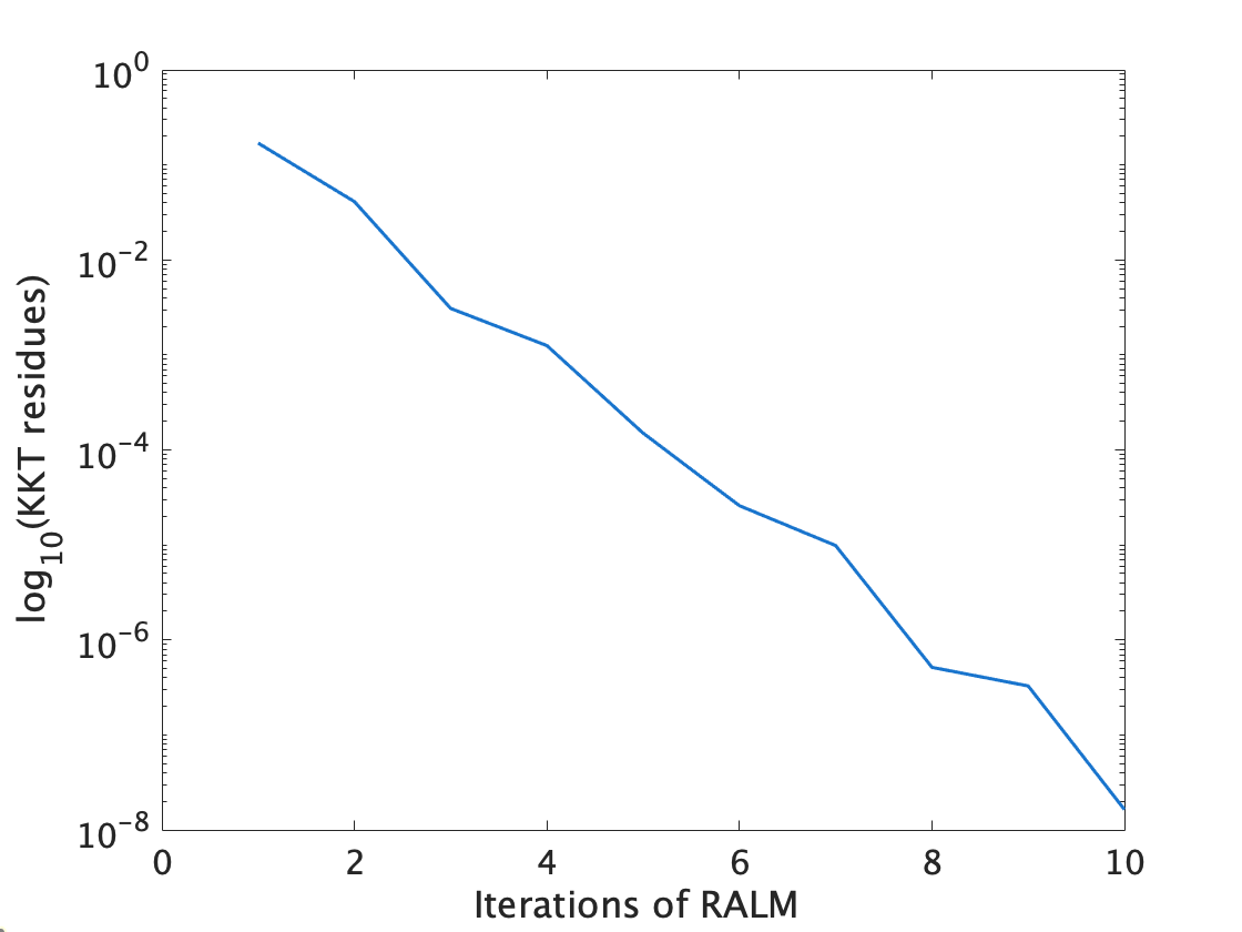
Figure 1: KKT residues of the RMC problem generated by inexact RALM 




7.2 Compressed modes


In this section, we will consider the compressed modes (CM) problem. Let $H$ be a discretization of the Hamilton operator, then the CM problem is formulated as follow ([29]):



(40)

$$\begin{array}[]{ll}\min_{X\in\mathbb{R}^{n\times r}}&\operatorname{tr}(X^{\top}HX)+\mu\left\|X\right\|_{1}\\
\text{ s.t. }&X\in\operatorname{St}(n,r).\end{array}$$



By setting $f(X)=\operatorname{tr}(X^{\top}HX)$, $\theta=\mu\|\cdot\|_{1}$, $g(X)=X$ and $\mathcal{M}=\operatorname{St}(n,r)=\{X|X^{\top}X=I_{r}\}$, this is of the form of (1).
The tangent space of $\mathcal{M}=\operatorname{St}(n,r)$ at $X$ is



(41)

$$T_{X}\mathcal{M}=\left\{\xi\in\mathbb{R}^{n\times r}:X^{\top}\xi+\xi^{\top}X=0\right\},$$



and the
the projection to tangent space is given by $\Pi_{X}Y=Y-X\operatorname{sym}(X^{\top}Y)$.
The Lagrangian of (40) can be written as $L(X,y)=\operatorname{tr}(X^{\top}HX)+\left\langle X,y\right\rangle$. Then the KKT condition is



(42)

$$\left\{\begin{array}[]{l}\Pi_{X}(2HX+y)=0,\\
y\in\mu\partial\|X\|_{1}.\end{array}\right.$$





The Euclidean gradient of $L(X,y)$ is $\nabla_{X}L(X,y)=2HX+y$,
and for any $\xi\in T_{X}\mathcal{M}$, the Euclidean Hessian of $L(X,y)$ is
$\nabla_{XX}^{2}L(X,y)[\xi]=2H\xi$.
Therefore, by [20] the Riemannian gradient and Hessian of $L(X,y)$ can be computed as




$$\operatorname{grad}L(X,y)
=\Pi_{X}(2HX+y),$$





$$\operatorname{Hess}L(X,y)\xi
=\Pi_{X}(2H\xi-\xi\operatorname{sym}(X^{\top}\nabla_{X}L(X,y)).$$




Moreover, for any $\xi\in T_{w}\mathcal{M}$, we have



(43)

$$\left\langle\xi,\operatorname{Hess}L(w,y)\xi\right\rangle
=\left\langle\xi,2H\xi-\xi\operatorname{sym}(X^{\top}\nabla_{X}L(X,y)\right\rangle$$






$$=\left\langle\xi,2H\xi\right\rangle-\left\langle\xi,2\xi X^{\top}HX\right\rangle-\left\langle\xi,\xi\operatorname{sym}(X^{\top}y)\right\rangle.$$




By the KKT condition (42), we have $2HX+y\in N_{X}\mathcal{M}$. Equivalently, there exists a symmetric matrix $S$, such that $2HX+y=XS$. Combining with (43) we can obtain




$$\left\langle\xi,\operatorname{Hess}L(w,y)\xi\right\rangle
=\left\langle\xi,2H\xi\right\rangle-\left\langle\xi,2\xi X^{\top}HX\right\rangle-\left\langle\xi,\xi\operatorname{sym}\left(X^{\top}(XS-2HX)\right)\right\rangle$$






$$=\operatorname{tr}(\xi^{\top}H\xi)-\operatorname{tr}(\xi^{\top}\xi S).$$



We further obtain the critical cone of $\theta$ and $g$ as $\mathcal{C}_{\theta,g}(X,y)=\{d\in\mathbb{R}^{n\times r}|\theta^{\prime}(X,d)=\left\langle d,y\right\rangle\}$, where




$$\theta^{\prime}(X;d)=\sum_{X_{ij}=0}|d_{ij}|+\sum_{X_{ij}>0}d_{ij}-\sum_{X_{ij}<0}d_{ij}.$$



The affine hull of $\mathcal{C}_{\theta,g}(X,y)$ is then given by




$$\operatorname{aff}\mathcal{C}_{\theta,g}(X,y)=\left\{d\in\mathbb{R}^{n\times r}|d_{ij}=0\;\text{if}\;y_{ij}\neq\pm\mu,\;d_{ij}\in\mathbb{R}\;\text{if}\;y_{ij}=\pm\mu\right\}.$$



Therefore, the M-SSOSC for CM problem at the KKT point $(\bar{X},\bar{y})=(\bar{X},-2H\bar{X}+\bar{X}\bar{S})$ holds if for any $\xi\in T_{\bar{X}}\mathcal{M}$ satisfying $\xi\in\operatorname{aff}\mathcal{C}_{\theta,g}(\bar{X},\bar{y})\backslash\{0\}$, $\operatorname{tr}(\xi^{\top}H\xi)-\operatorname{tr}(\xi^{\top}\xi\bar{S})>0$ holds.


In [42], the authors consider setting the CM problem to solve Schrödinger equation of 1D free-electron model with periodic boundary condition:



(44)

$$-\frac{1}{2}\Delta\phi(x)=\lambda\phi(x),\quad x\in[0,50]$$



and numerically, they find that the smallest eigenvalue of $H_{k}\in\partial\operatorname{grad}L^{\rho_{k}}\left(X_{k},y^{k}\right)$ is always larger than zero, which implies that the M-SSOSC may be satisfied in this case. Here we use a simple example to illustrate this conjecture.


Consider the Schrödinger equation of with boundary condition when $x\in[0,2]$. Discretize the domain$[0,2]$ into $n=4$ nodes and let $H$ be the discretized version of $-\frac{1}{2}\Delta$. Then $H=-\small\begin{bmatrix}-4&2&0&2\\
2&-4&2&0\\
0&2&-4&2\\
2&0&2&-4\end{bmatrix}$. For $r=2$, it can be verified that $\bar{X}=\small\begin{bmatrix}0&0&\sqrt{2}/2&\sqrt{2}/2\\
\sqrt{2}/2&\sqrt{2}/2&0&0\end{bmatrix}^{\top}$ is a stationary point of (40), and one of the corresponding multiplier $\bar{y}$ is given by $\bar{y}=\mu\small\begin{bmatrix}0&0&1&1\\
1&1&0&0\end{bmatrix}^{\top}$. Moreover, if rewrite $\bar{y}=\bar{X}\bar{S}-2H\bar{X}$, then $\bar{S}=\small\begin{bmatrix}-4+\sqrt{2}\mu&4\\
4&-4+\sqrt{2}\mu\end{bmatrix}$. The affine hull of $\mathcal{C}_{\theta,g}(\bar{X},\bar{y})$ is now written as
$\operatorname{aff}\mathcal{C}_{\theta,g}(\bar{X},\bar{y})=\left\{\begin{bmatrix}0&0&\xi_{1}&\xi_{2}\\
\xi_{3}&\xi_{4}&0&0\end{bmatrix}^{\top}\Big{|}\xi_{i}\in\mathbb{R},i=1,2,3,4\right\}$.
For any $\xi\in\operatorname{aff}\mathcal{C}_{\theta,g}(\bar{X},\bar{y})$ satisfying $\xi\in T_{\bar{X}}\mathcal{M}$, by (41) we further obtain $\xi=\small\begin{bmatrix}0&0&\xi_{1}&-\xi_{1}\\
\xi_{2}&-\xi_{2}&0&0\end{bmatrix}^{\top}$. Therefore, for any $\xi\in T_{\bar{X}}\mathcal{M}$ satisfying $\xi\in\operatorname{aff}\mathcal{C}_{\theta,g}(\bar{X},\bar{y})\backslash\{0\}$, we have




$$\operatorname{tr}(\xi^{\top}H\xi)-\operatorname{tr}(\xi^{\top}\xi\bar{S})=12(\xi_{1}^{2}+\xi_{2}^{2})-2(-4+\sqrt{2}\mu)(\xi_{1}^{2}+\xi_{2}^{2})=(20-2\sqrt{2}\mu)(\xi_{1}^{2}+\xi_{2}^{2}).$$



As long as $\mu<5\sqrt{2}$, the M-SSOSC is satisfied for this problem. From Corollary 6.4, the general Jacobian used in the semisooth newton is positve definite. Now setting $\mu=0.8$ and apply RALM, we obtain Figure 2, which shows the linear rate of KKT residue.


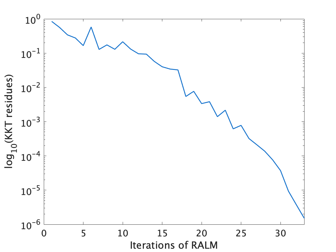
Figure 2: KKT residues of CM generated by inexact RALM 


For larger $n$ and $r$, it seems difficult to prove the positive definiteness of the general Hessian used in Algorithm 1. However, The minimal eigenvalue is observed to be positive in [42, Table 5].
We also consider back to problem (44) with shifting $n$ nodes and similarly observe that the smallest eigenvalues of the general Hessians used in the semismooth Newton methods are positive.


Table 1: The minimum eigenvalue of the general Hessian which is used in Algorithm 1 for (40).



n
r
mimimum eigenvalue




200
20
0.3049
0.3238
0.1926
0.2811
0.1447


500
20
0.2755
0.1089
0.1173
0.0982
0.1087


1000
20
0.0266
0.1658
0.0026
0.1684
0.2055








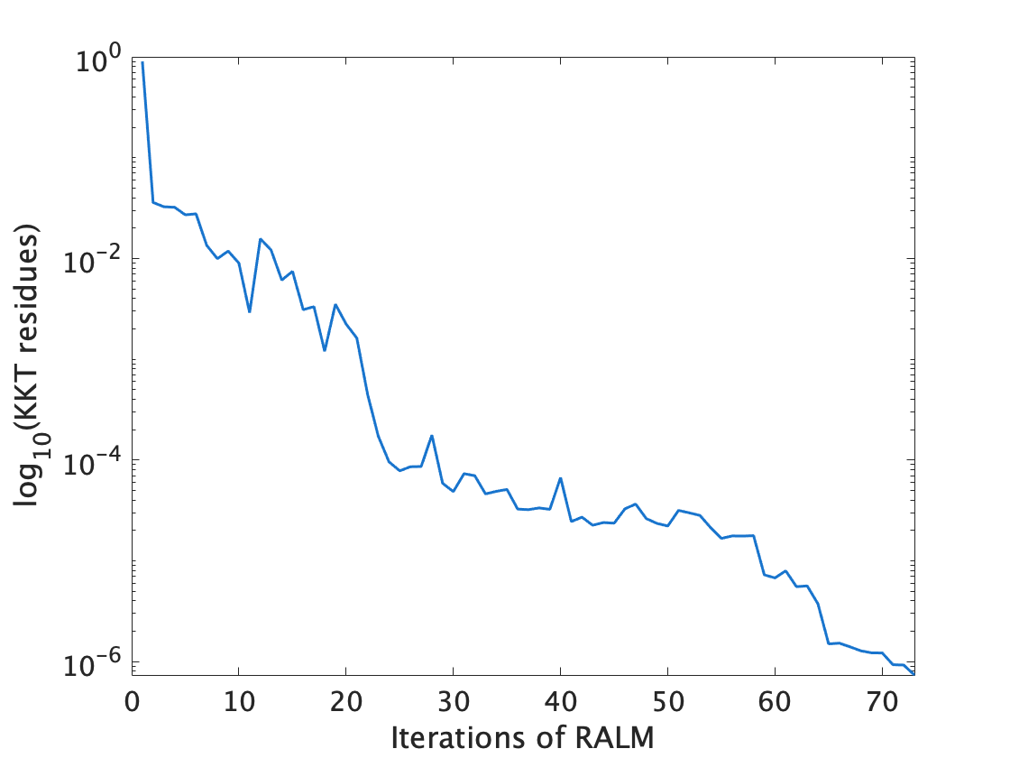
(a) n=200, r=20




(b) n=500, r=20




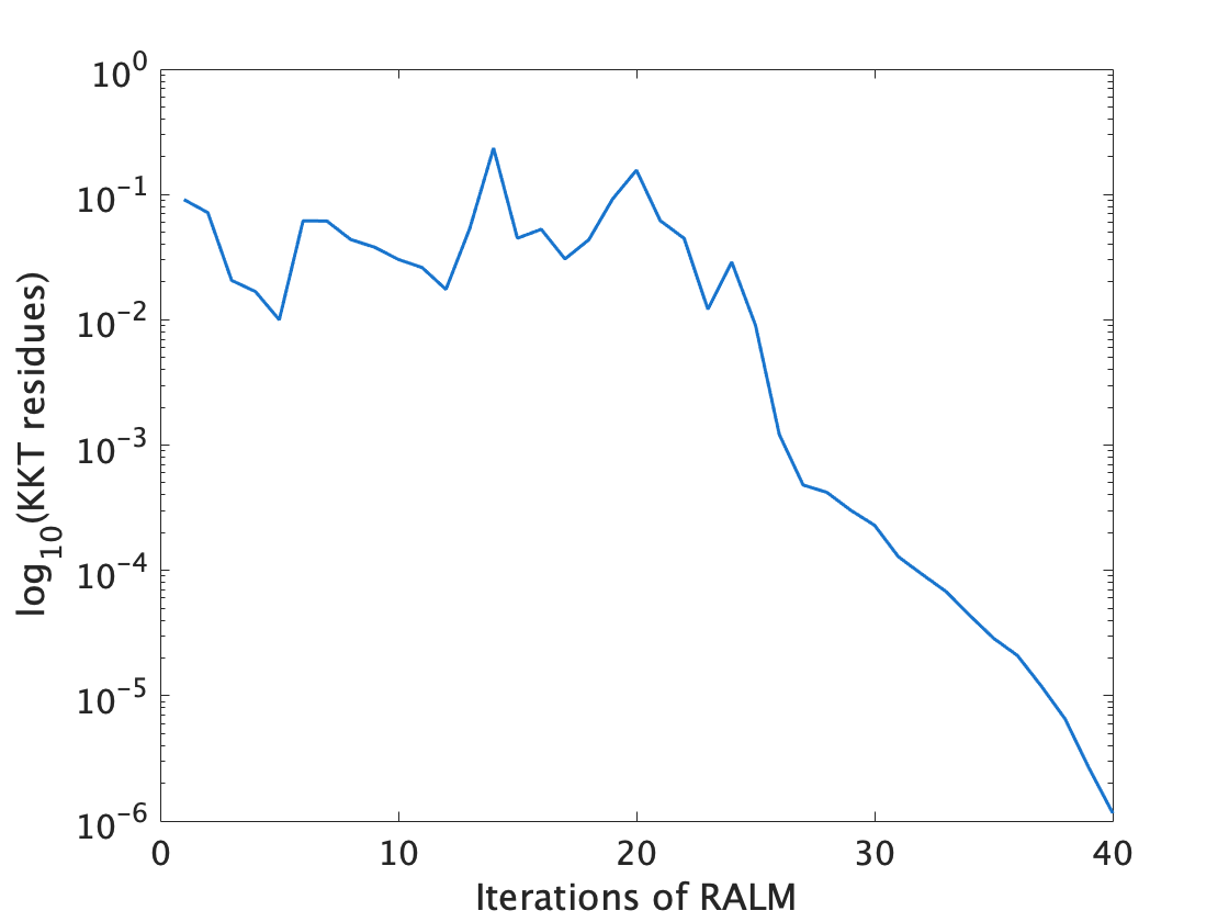
(c) n=1000, r=20



Figure 3: The KKT residues of compressed modes problems generated by inexact RALM


Table 1 indicates that the manifold strong variational sufficiency might be satisfied at the obtained points. Therefore, we consider applying the RALM and all settings follow [42]. The results of variations in KKT residues are reported in Figure 3.



8 Conclusion


This paper investigates the local convergence of RALM without assuming the uniqueness of multiplier. We devise a local equivalent problem on tangent space and introduce the manifold variational sufficient condition. It is shown that manifold strong variational sufficient condition is equivalent to the M-SSOSC under certain circumstances. Under this condition, a local augmented dual problem is formulated, consequently establishing the linear convergence rate of RALM. Furthermore, we prove that general Hessians used in the semismooth Newton method for solving the RALM subproblem are positive definite when the manifold strong variational sufficiency holds. The numerical experiments on various applications demonstrate the linear convergence rate.


However, there remain several unresolved issues in Riemannian nonsmooth optimization. For instance, verifying the retractional convexity for manifold functions presents a significant challenge and is waiting for future study. Additionally, while it is understood that the primal proximal point algorithm is equivalent to the dual ALM in Euclidean settings, the relationship between these two algorithms remains unknown under the retactional convexity in a Riemannian setting.

References

[1]P.-A. Absil and S. Hosseini, A collection of nonsmooth Riemannian
optimization problems, Nonsmooth Optimization and Its Applications,
(2019), pp. 1–15.
[2]P.-A. Absil, R. Mahony, and R. Sepulchre, Optimization algorithms
on matrix manifolds, Princeton University Press, 2009.
[3]P.-A. Absil and J. Malick, Projection-like retractions on matrix
manifolds, SIAM Journal on Optimization, 22 (2012), pp. 135–158.
[4]D. Azagra, J. Ferrera, and F. López-Mesas, Nonsmooth analysis
and Hamilton–Jacobi equations on Riemannian manifolds, Journal of
Functional Analysis, 220 (2005), pp. 304–361.
[5]D. P. Bertsekas, Constrained optimization and Lagrange multiplier
methods, Academic press, 2014.
[6]N. Boumal, An introduction to optimization on smooth manifolds,
Cambridge University Press, 2023.
[7]L. Cambier and P.-A. Absil, Robust low-rank matrix completion by
Riemannian optimization, SIAM Journal on Scientific Computing, 38 (2016),
pp. S440–S460.
[8]S. X. Chen, Z. D. Deng, S. Q. Ma, and A. M.-C. So, Manifold
proximal point algorithms for dual principal component pursuit and orthogonal
dictionary learning, IEEE Transactions on Signal Processing, 69 (2021),
pp. 4759–4773.
[9]S. X. Chen, S. Q. Ma, A. M.-C. So, and T. Zhang, Proximal gradient
method for nonsmooth optimization over the Stiefel manifold, SIAM Journal
on Optimization, 30 (2020), pp. 210–239.
[10]A. R. Conn, N. I. M. Gould, and P. L. Toint, Trust region
methods, SIAM, 2000.
[11]F. R. de Oliveira and O. P. Ferreira, Newton method for finding a
singularity of a special class of locally Lipschitz continuous vector fields
on Riemannian manifolds, Journal of Optimization Theory and Applications,
185 (2020), pp. 522–539.
[12]L. Demanet and P. Hand, Scaling law for recovering the sparsest
element in a subspace, Information and Inference: A Journal of the IMA, 3
(2014), pp. 295–309.
[13]K. K. Deng and Z. Peng, An inexact augmented Lagrangian method for