PV-SSD: A Multi-Modal Point Cloud Feature Fusion Method for Projection Features and Variable Receptive Field Voxel Features

Abstract

LiDAR-based 3D object detection and classification is crucial for autonomous driving. However, real-time inference from extremely sparse 3D data is a formidable challenge. To address this problem, a typical class of approaches transforms the point cloud cast into a regular data representation (voxels or projection maps). Then, it performs feature extraction with convolutional neural networks. However, such methods often result in a certain degree of information loss due to down-sampling or over-compression of feature information. This paper proposes a multi-modal point cloud feature fusion method for projection features and variable receptive field voxel features (PV-SSD) based on projection and variable voxelization to solve the information loss problem. We design a two-branch feature extraction structure with a 2D convolutional neural network to extract the point cloud’s projection features in bird’s-eye view to focus on the correlation between local features. A voxel feature extraction branch is used to extract local fine-grained features. Meanwhile, we propose a voxel feature extraction method with variable sensory fields to reduce the information loss of voxel branches due to downsampling. It avoids missing critical point information by selecting more useful feature points based on feature point weights for the detection task. In addition, we propose a multi-modal feature fusion module for point clouds. To validate the effectiveness of our method, we tested it on the KITTI dataset and ONCE dataset.

I Introduction

At this stage, AI-related technologies are constantly developing applications are emerging. As an important part of the perception layer of autonomous driving, efficient object detection methods can provide a solid foundation for behavioral decisions in autonomous driving. Object detection methods need to detect moving objects such as cars, pedestrians, and cyclists in the current environment in real time and accurately detect their location and orientation. Although significant progress has been made in image-based 2D object detection[1, 2, 3, 4, 5, 6, 7, 8, 9] at this stage, compared with 3D space, 2D space lacks depth information. It cannot accurately describe the position and orientation of objects. The subsequently proposed depth camera-based [10, 11, 12, 13] and [mult020disp, 14, 15, 16] make up for the lack of depth information from 2D cameras. Still, the cameras are sensitive to the light environment and often perform poorly in complex urban environments. Compared to images, LIDAR enables easier description of object poses in 3D space. Unlike images, point clouds have separate objects without occlusion, thereby eliminating the occlusion problem. Additionally, LIDAR is more robust to illumination changes[17, 18, 19, 20, 21].

However, there are some challenges in point cloud-based 3D object detection methods. For example, (1) sparsity; (2) disorder; and (3) rotation invariance [19]. Currently, the existing methods can be mainly categorized into point-based [22, 23],projection-based [24, 25, 26, 27], and voxel-based[28, 29]. Point-based methods extract features directly from the raw point cloud. However, point-based methods often lead to discontinuities between feature points during feature sampling, thus ignoring the correlation between fine-grained local features. Projection-based and voxel-based methods first encode the fine-grained local features within the same mesh and then perform feature extraction with convolutional neural networks, preserving the correlation between local features as much as possible. However, projection-based methods can lose the amount of point cloud features by over-compressing them in one direction during data processing[30]. On the other hand, although the voxel-based methods avoid compression of the point cloud features in a certain direction, the 3D convolutional neural network can also lead to the lack of fine-grained information during the downsampling process.

To address these issues, this paper proposes a multi-modal point cloud feature fusion method for projection features and variable receptive field voxel features (PV-SSD). We designed a dual-branch feature extraction structure: the projection branch utilizes 2D convolutional neural networks to extract projection features of point clouds from a bird’s eye view, focusing on the correlation among local features, and the voxel feature branch extracts fine-grained local features. Simultaneously, to partially compensate for the feature loss in the projection branch, we employed a voxel feature extraction structure called Variable Receptive Field Voxel Feature Extraction (VR-VFE). VR-VFE uses fully connected layers to extract local features from individual voxels and selects more useful feature points for detection tasks based on feature point weights, aiming to retain key feature points as much as possible during downsampling. Furthermore, within VR-VFE, we introduced a Point-wise Feature Weighting Network (PWF-Net) to remove redundant features introduced during feature dimension expansion in the feature extraction process. Experimental results demonstrate that VR-VFE enables our method to perform well on objects with fewer reflective points, such as ’Cyclist.’ In the neck network, we improved the Spatial Semantic Feature Aggregation (SSFA) module proposed in CIA-SSD [31]. We introduced feature inputs with different resolutions and proposed a multi-modal spatial feature fusion method (MSP-Fusion) to further fuse features with the same index and their adjacent features from different modalities. Compared to using multi-view projections in H²3D R-CNN [32] to compensate for the information loss, the voxel branch contains more fine-grained local features. This dual-branch structure of voxels and projections is more conducive to detecting small targets or distant objects. Moreover, compared with the perspective view, the voxelized point cloud is not affected by the occlusion problem. To address the information loss problem due to downsampling, SMS-Net [33] proposes a method for aggregating multi-scale voxel features. [34] designs a two-stage 3D detector that uses the candidate regions generated in the first stage for feature aggregation in the original point cloud. However, in the autopilot scenario, the number of foreground points is small, and these methods inevitably result in missing foreground points during the downsampling process. The VR-VFE structure proposed in this paper can be sampled according to the weights of the feature points, retaining as much as possible the feature points that are more favorable for the detection task.

In summary, we make three-fold contributions:

• A two-branch feature extraction network for multimodal features of point clouds is proposed

• A voxel feature extraction method with variable receptive fields is proposed.

• Improving the SSFA module proposed in CIA-SSD [31] by proposing the Multi-modal Spatial-Semantic Feature Aggregation (MSSFA) module.

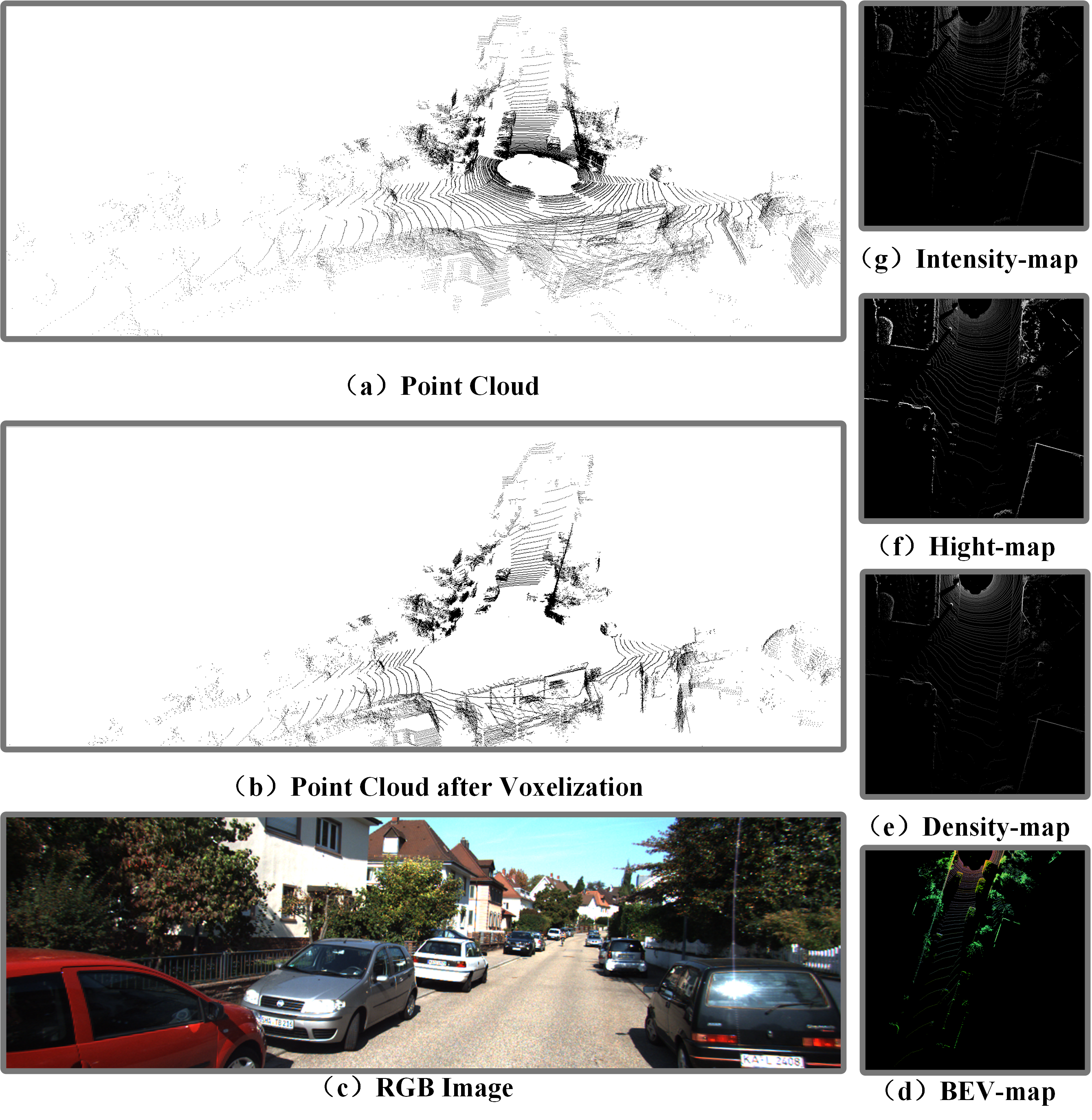
Figure 1: An illustration of (a) Point Cloud, (b)Point Cloud after voxelization, (c) RGB Image, (d) BEV-map, (e) Density-map, (f) Hight-map, and (g) Intensity-map. Each voxel in (b) contains 12 points, and the size of the voxel is [0.1m,0.1m, 0.125m]. Density-map, Height-map, and Intensity-map are the three channels of BEV-map. Each pixel in the density map, height map, and intensity map represents the normalized density of the point cloud, the maximum height of the point cloud, and the maximum intensity of the point cloud in that grid point, respectively.

II Related Work

3D object detection based on LiDAR point cloud can be classified into point-based, voxel-based and projection-based methods depending on the data pre-processing method.

II-A Point-based 3D object detection methods

Point-based methods usually choose to directly feature extract the raw point cloud and learn the spatial structure features of the point cloud. But, considering the disorderly nature of point cloud data and other characteristics, such methods usually choose PointNet [19] or PointNet++ [20] for feature extraction. F-PointNet [18] uses the 2D candidate bounding box generated from RGB images to generate a frustum. Then it uses PointNet++ to extract features from the point cloud in the frustum and to perform subsequent classification and regression. PointRCNN[22] is the first point-based two-stage 3D object detection algorithm. It classifies the point cloud in the first stage for foreground and background, then generates 3D candidate bounding box. The second stage further classifies and regresses the detection results of the first stage. STD [23] proposes a two-stage algorithm from sparse to dense, which uses a spherical anchor to generate candidate frames in the first stage to achieve high recall, and a parallel intersection-over-union (IoU) branch in the second stage to achieve high accuracy. PV-RCNN [30] proposes a novel detection framework by combining the advantages of variable perceptual fields of point-based methods with the advantages of efficient feature extraction capabilities of voxel-based methods.

II-B Voxel-based 3D object detection method

VoxelNet [28] proposed a method to transform disordered point clouds into regular voxel, then completed the feature extraction and detection tasks with 3D convolution. SECOND [29] proposed a more efficient 3D convolutional feature extraction method called sparse convolution. Voxel R-CNN [35] extends VoxelNet into a two-stage method and proposes the Voxel ROI Pooling method for feature aggregation. PartA² [36] further explores the spatial distribution characteristics of different parts of objects in the annotation frames. It adds the prediction of information about the internal position distribution of foreground objects in the first stage. SA-SSD [37] proposes an auxiliary network that can be turned off anytime to improve the information loss problem due to downsampling in the feature extraction stage. CIA-SSD [31]] used IoU-aware confidence rectification module and Multi-task head module to enhance the problem of imbalance between classification confidence and regression confidence in 3D detection tasks. SARPNET [38] compensates for the sparsity and inhomogeneity of point clouds through a uniform sampling method, and enhances the learning of object 3D shape features and spatial semantic features through a shape attention mechanism. DVFENet [39] proposed a two-branch detection method based on an improved voxel graph attention feature extractor (VGAFE) and 3D sparse convolutional networks, which can provide rich 3D feature information. SMS-Net [33] proposed a sparse multi-scale voxel feature aggregation network that divides the raw point cloud into voxels of different sizes to perceive 3D features under different sensory fields.

II-C Projection-based 3D object detection method

Projection-based methods usually project disordered point clouds to different viewpoints, transform them into regular pseudo-image representations, and complete subsequent feature extraction and detection tasks with 2D convolution. MV3D, AVOD, etc. [24, 25, 32, 40, 41, 26, 27], transform the point cloud projection into a height, density, and intensity map for feature extraction. Among them, MV3D and AVOD [32, 40, 41] use multi-view fusion, while Complex-YOLO and YOLO3D [24, 27] perform feature extraction and detection in a bird’s eye view. However, this excessive compression of point cloud information by single view leads to a large amount of feature information loss, which is not conducive to the detection task. PointPillars [26] converts the point cloud into a top-down pillar, then generates a pseudo-image in the bird’s-eye view after completing feature encoding on the pillar, which reduces the feature information loss to a certain extent. H²3D-RCNN [32] adopts the same feature encoding method as PointPillars, which combines the advantages of the dense point cloud in perspective view and unobstructed bird’s-eye view to improve the detection accuracy further.

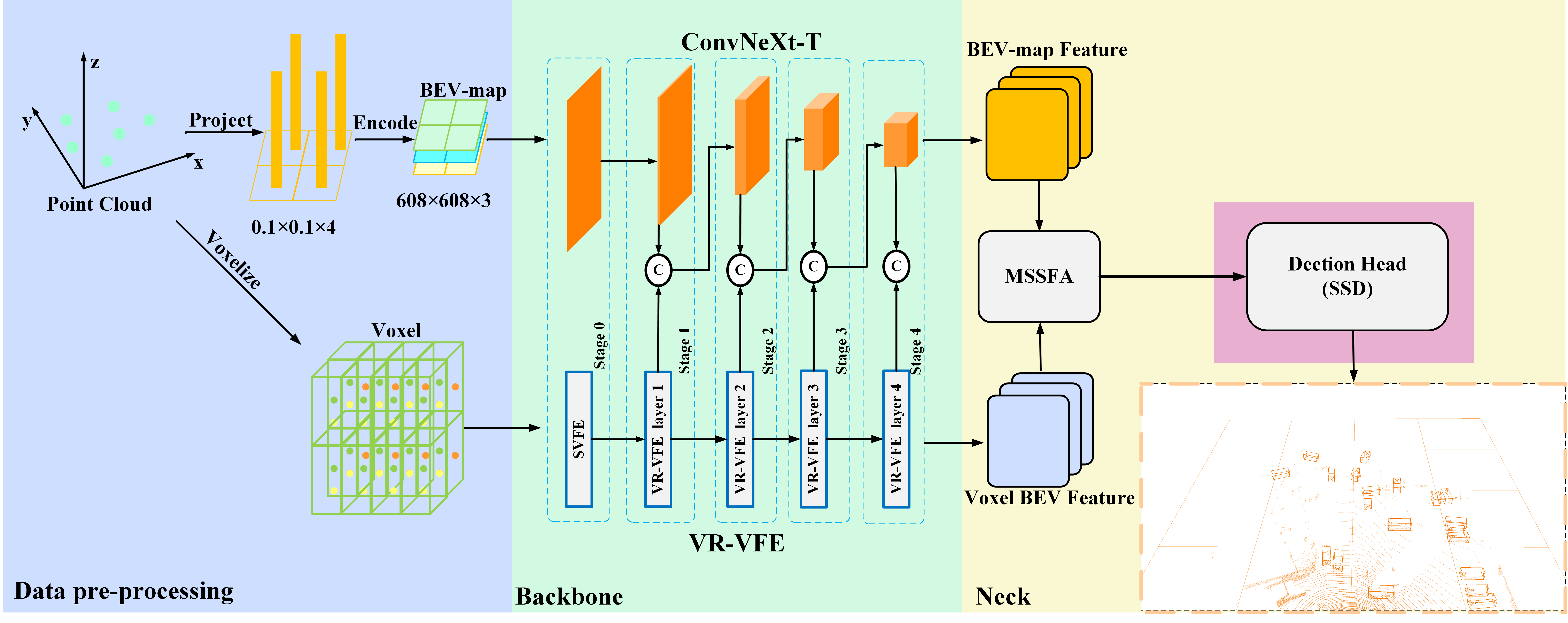
Figure 2: Algorithm flow. Where ’C’ denotes concatenation operation (stitching by feature dimension). The point cloud data are transformed into BEV-map and voxel as input, the BEV-map feature is extracted with ConvNeXt-Tiny, and the voxel features are extracted with VR-VFE proposed in this paper. Multi-scale feature fusion is performed in MSSFA. Finally, the 3D detection is done in SSD Detection Head. ’$0.1\times 0.1\times 4$’ refers to the size of each grid corresponding to reality after meshing the point cloud. ’$608\times 608\times 3$’ refers to the size of the BEV-map generated by the projection.

III Methodology

III-A Overview

Fig. 1. shows the form of the data covered in this paper. Fig. 1. (d) shows the BEV-map, while Fig.1. (e)-(g) display its components; Fig.1. (a) shows the raw point cloud; Fig.1. (b) shows the Voxel; Fig.1. (C) shows the RGB Image. Our method consists of four parts, the flowchart is shown in Fig. 2.

• Data pre-processing: we use two different data pre-processing methods to obtain 2D pseudo-images of the bird’s eye view (from now on, we call them BEV-map) and voxelized point cloud data.

• Backbone network: we feed the BEV-map into the 2D convolutional neural network and the voxelized point cloud data into the voxel feature extraction network to complete the feature extraction.

• Neck network: the BEV-map feature and the voxel features are fused with the features.

• Detection head: classify and regress 3D bounding boxes.

III-B Data pre-processing

Considering that the farther away from the LiDAR, the sparser the obtained point cloud. Therefore, we selected the point cloud within the range of $x\in\left[-30.4m,30.4m\right]$ and $y\in\left[0m,60.8m\right]$. Considering height of LiDAR above the ground and the problem of occlusion, we selected point cloud within the range of $z\in\left[-3m,1m\right]$. Here we define $P_{\Omega}$ as the set of point clouds, we adopt.

$$P_{\Omega}=\left\{P=\left[x,y,z\right]^{T}\right\}\\ x\in\left[0m,60.8m\right],y\in\left[-30.4m,30.4m\right],z\in\left[-3m,1m\right]$$ (1)

Bev-map: We adopt the same data pre-processing method as Complex-YOLO [22], where the single-frame point cloud data in $P_{\Omega}$ is converted into pseudo-images in bird’s-eye view. The maximum height, maximum intensity, and point cloud density in bird’s-eye view will be encoded and filled into the corresponding channels. The final size of BEV-map is $608\times 608\times 3$, and each pixel corresponds to a realistic range of $\left[0.1m,0.1m,4m\right]$. The three channels of the BEV-map are encoded by the following (2), (3), and (4).

$$z_{g}=max(P_{\Omega i\longrightarrow j}\cdot\left[0,0,1\right]^{T})$$ (2)

$$z_{b}=max(I(P_{\Omega i\longrightarrow j}))$$ (3)

$$z_{r}=min(1.0,log(N+1)/log(64))\quad N=\left|P_{\Omega i\longrightarrow j}\right|$$ (4)

In the above (2), (3), and (4), $z_{g}$ represents the maximum height; $z_{b}$ represents the maximum intensity; $z_{r}$ represents the normalized density; $I(P_{\Omega})$ represents the point cloud intensity; and $N$ represents the number of point clouds in each grid.

Voxel: We will voxelize the single-frame point cloud data in $P_{\Omega}$, using the same feature encoding as in PointPillars[26]; each point cloud in the voxel will be encoded as a 10-dimensional vector D: $\left(x,y,z,r,x_{c},y_{c},z_{c},x_{p},y_{p},z_{p}\right)$.where $x,y,z,r$ represent the 3-dimensional coordinates of the point cloud and the reflection intensity, $x_{c},y_{c},z_{c}$ represent the geometric centers of all points in the voxel in which the point cloud is located, and $x_{p},y_{p},z_{p}$ are $x-x_{c},y-y_{c},z-z_{c}$, which represent the relative positions of the points to the geometric centers. Due to the sparsity of the point cloud, most of the sets of voxels are empty, while the non-empty voxels often have only a few points. This sparsity is exploited by imposing limits on the number of non-empty voxels per sample $(V)$ and the number of point clouds per voxel (N) to create a dense tensor of size $(D,V,N)$. The data will be randomly sampled if a voxel has too many points to fit in this tensor. Conversely, if a voxel has too few points, it will be filled with zeros [26].

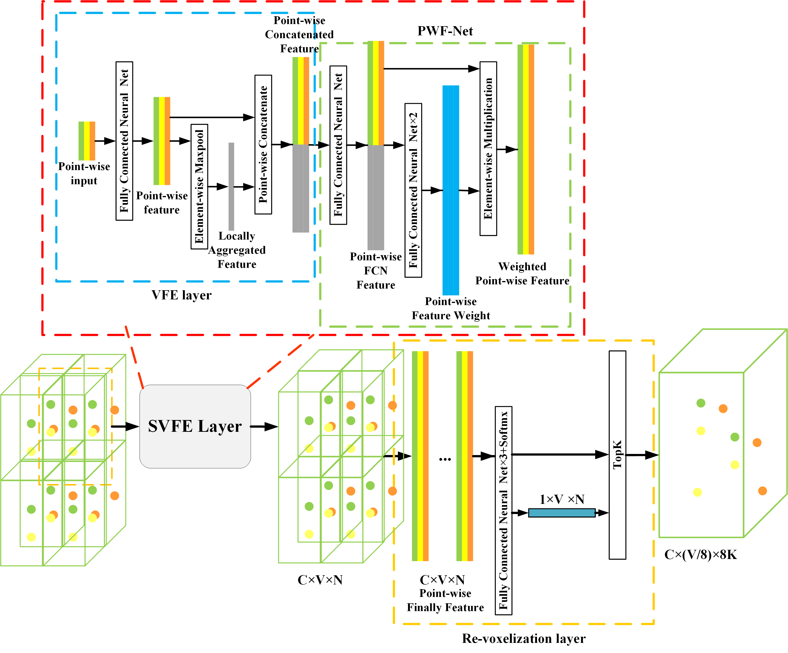
Figure 3: We present the VR-VFE layer structure with downsampling along the x, y, and z axes. The red dashed box part is SVFE module; the blue dashed box part is VFE module; the green dashed box part is PFW-Net; the yellow dashed box part is Re-voxelization layer. In ’$C\times V\times N$’, ’$V$’ denotes the number of voxels, ’$N$’ denotes that each voxel contains N point-wise, and ’$C$’ denotes the number of features in each point-wise.

III-C Backbone

The backbone consists of BEV-map feature extraction network, voxel feature extraction network, and feature fusion.

Projection Branch: We use ConvNeXt [42] as a feature extraction network for BEV-map, which is a feature extraction network proposed by Zhuang Liu et al. in 2022. ConvNeXt made a series of improvements to ResNet [43] by borrowing some module designs from Transformer [44, 45] (e.g., replacing ReLU layer with GeLU layer, replacing Batch Normalize layer with Layer Normalize layer, etc.). In this paper, we use ConvNeXt-Tiny, a lighter version of ConvNext, for feature extraction of BEV-map.

Voxel Branch: The voxel feature extraction part is stacked by the Variable Receptor Field Voxel Feature Extraction layer (VR-VFE layer). The VR-VFE layer consists of the modified Stacked Voxel Feature Encoding layer [28]] (SVFE layer) and Re-voxelization layer. There are five stages in CovNeXt-Tiny, where Stage 0 is mainly used for downsampling to reduce the subsequent computational overhead, and Stages 1 to 4 are used for further feature extraction (each stage downsamples the feature maps by a factor of 2). Correspondingly, in the voxel branch, we also designed five stages, where the first stage consists of an SVFE layer for expanding the channel dimension of the voxel features (it should be noted that the first stage does not perform a downsampling operation). Each of the subsequent Stages 1 to 4 consists of a VR-VFE layer, which is used for further feature extraction (each of Stages 1 to 4 is downsampled, with 4-fold downsampling for Stage 1 and 2-fold downsampling for Stages 2 to 4, to avoid misalignment of features in the projection branch). The structure of VR-VFE layer is shown in Fig. 3. The structure of SVFE is shown in the red dashed box in Fig. 3. The VFE structure is shown in the blue dashed box in Fig.3. The PFW-Net structure is shown in the green dashed box section of Fig. 3. The Re-voxelization layer structure is shown in the yellow dashed box section of Fig. 3.

SVFE is a voxel feature encoding layer proposed in VoxelNet [28]. The SVFE module used in this paper replaces the original structure with a new one consisting of a VFE layer, a Fully Connected Network layer (FCN, each FCN consists of a fully connected layer, a GeLU layer, and a Layer Normalize layer), and a Point-wise Feature Weighting Net (PWF-Net).

We use $VFE_{i}(c_{in},c_{out})$ to represent the VFE layer, where $c_{in}$ represents the input point-wise feature dimension and $c_{out}$ represents the output feature dimension. Firstly, it raises the feature dimension to $c_{out}\setminus 2$ by FCN to get the point-wise feature. The point-wise feature is then operated by element-wise MaxPool to obtain locally aggregated feature, and finally it is concatenated with the point-wise feature by feature dimension to obtain point-wise concatenated feature with feature dimension $c_{out}$.

During the voxel feature extraction process, we increase the channel dimension of feature points through fully connected layers to enable the extraction of richer semantic features in deep networks. However, as the channel dimension grows, features extracted in deeper layers of the network may contain redundant information that is irrelevant to the detection task. To address this issue, we introduce PFW-Net to highlight feature information that is more favorable for the detection task. PFW-Net can be seen as a simple self-attention mechanism that enables the network to focus more on features that are beneficial for object detection tasks. It computes the point-wise feature weight (between 0 and 1) using two fully connected layers and a Softmax layer, then multiplies it element-wise with the point-wise FCN feature to obtain the weighted point-wise feature. Additionally, during the network training phase, the loss function implicitly supervises network parameters, such as the weights and biases of fully connected layers and convolutional layers. This enables PFW-Net to derive a contribution value between 0 and 1 for each feature point similar to its importance to the final detection task. Subsequently, these contribution values are element-wise multiplied with the feature points to emphasize those that are more beneficial to the final detection task. In the subsequent ablation experiments, we further demonstrated the effectiveness of PWF-Net through empirical testing.

In the feature extraction process, we transform the voxelized point-wise features into Voxel-BEV features in the bird’s-eye view for feature fusion with BEV-map features. However, each stage in the feature extraction of BEV-map involves a downsampling operation. For example, in ConvNeXt, stage 0 will do 4x downsampling for the feature map. The resolution corresponding to $608\times 608$ in this paper will become $152\times 152$, while the size of each grid point corresponding to the original point cloud will become $\left[0.4m,0.4m,4m\right]$. At the same time, the SVFE layer will not change the size of each voxel. Therefore, we designed the Re-voxelization layer to ensure that the Voxel-BEV features at each stage have the same resolution as BEV-map features. On the other hand, as the network deepens, such operations can make the point-wise features in each voxel contain the richer semantic feature.

For the detection task of objects with few reflection points (e.g., cyclists), it is especially important to use a limited number of feature points to complete the feature extraction. In the sampling process, we want to be able to sample each point in the voxel according to its significance for the detection task, so we design a sampling method based on the weight of each point. We obtain the weight value of each point by changing the feature number of the new point-wise feature to 1 through three fully connected layers and changing its value to between 0 and 1 by performing Softmax operation on the feature dimension. Finally, the top K points in each voxel before are selected according to the weight value magnitude as the point-wise in each voxel after the Re-voxelization layer. For example, if the original voxel contains 12 point-wise points and the voxel size is $\left[0.1m,0.1m,0.125m\right]$, we hope that after the Re-voxelization layer, each voxel contains 32 point-wise points. After the layer, each voxel contains 32 point-wise, and the voxel size is $\left[[0.4m,0.4m,0.25m\right]$. The first 4 points in each voxel will be selected according to the weight value (in this paper, we tend to select more points in the original voxel to increase the robustness of the network and then perform random sampling). After the sampling, to enhance the Point-wise spatial features in the resampled voxels, we encode the $\left(x,y,z,r\right)$ of these points corresponding to the points in the original point cloud with the same features as before to obtain $\left(x,y,z,r,x_{c},y_{c},z_{c},x_{p},y_{p},z_{p}\right)$, and stitch them with point-wise by feature dimension to obtain the new point-wise.

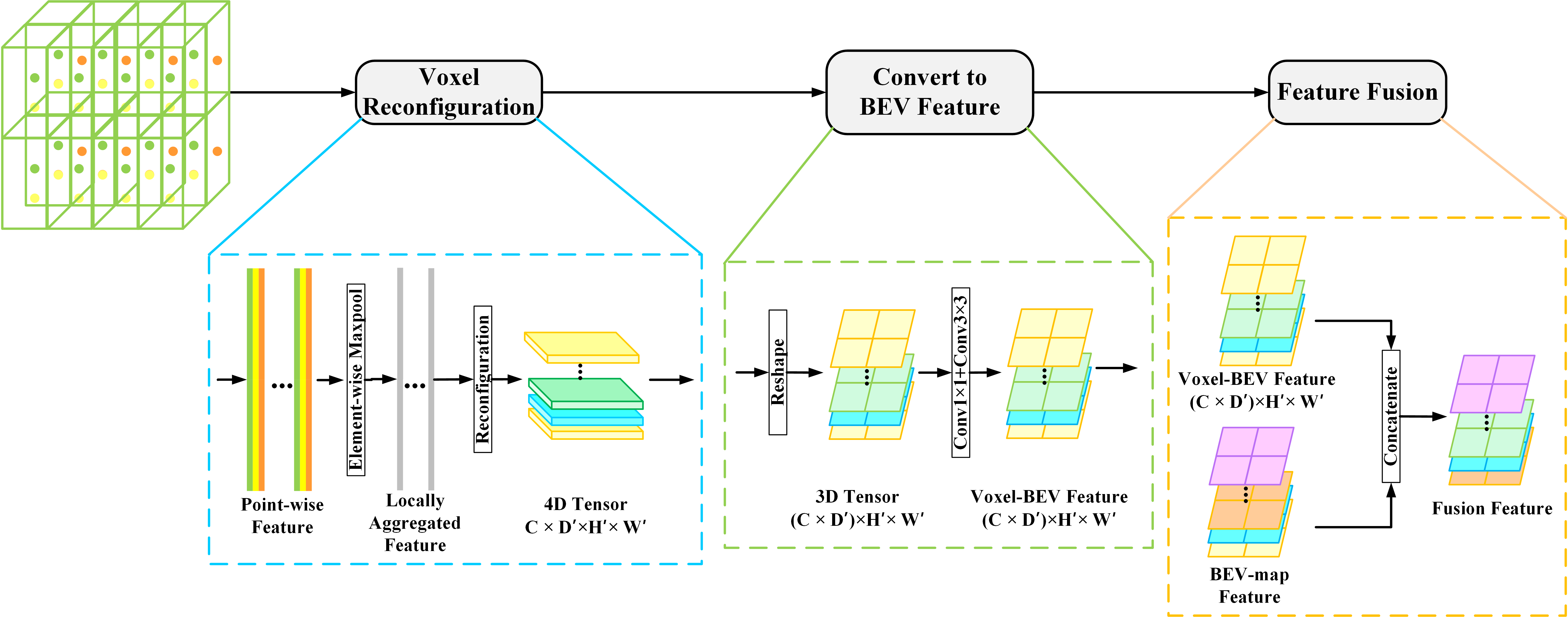
Figure 4: Feature fusion in the backbone. The blue dashed box shows the process of reconstructing the voxels into a 4D tensor. The green dashed box part transforms the reconstructed 4D tensor into a voxel feature map in the bird’s eye view. The yellow dashed box part fuses the BEV-map features with the Voxel BEV features for feature fusion.

Feature Fusion: In feature fusion, we first take the point-wise features (stored as $(C,V,N)$) in the voxels of each stage and get the local features (stored as $(C,1,N)$) that can represent each voxel through the element-wise MaxPool. The local voxel features are then reconstructed from $(C,1,N)$ into a sparse 4D tensor of size $(C,D^{{}^{\prime}},H^{{}^{\prime}},W^{{}^{\prime}})$, where $H^{{}^{\prime}}$, $W^{{}^{\prime}}$ represents the resolution of voxel features and $D^{{}^{\prime}}$ represents the depth of voxel features. This 4D tensor is then reshaped into a 3D tensor of size $((C\times D^{{}^{\prime}}),H^{{}^{\prime}},W^{{}^{\prime}})$, and adjusted to a Voxel-BEV feature with a $1\times 1$ convolution and a $3\times 3$ convolution(the 3D voxel features will be transformed into 2D Voxel-BEV features by a $1\times 1$ convolution and a $3\times 3$ convolution to avoid the problem due to the misalignment of 3D voxel features with 2D BEV-map features.), and finally, the BEV-map feature obtained from the same Stage as ConvNeXt is stitched by feature dimension. The feature fusion is completed by a $1\times 1$ convolution and a $3\times 3$ convolution, and the subsequent feature extraction is performed. It should be noted that we did not perform feature fusion on the features of Stage 0 considering that the main purpose of Stage 0 of ConvNeXt is to reduce computational consumption and not to perform too much feature extraction. In addition, if feature fusion is performed on the features of Stage 0, we need to create a tensor of$608\times 608\times C$ ($C$ is the number of channels) in the subsequent MSP-Fusion structure of MSSFA, which will bring a very large computational consumption. The specific structure is shown in Fig. 4.

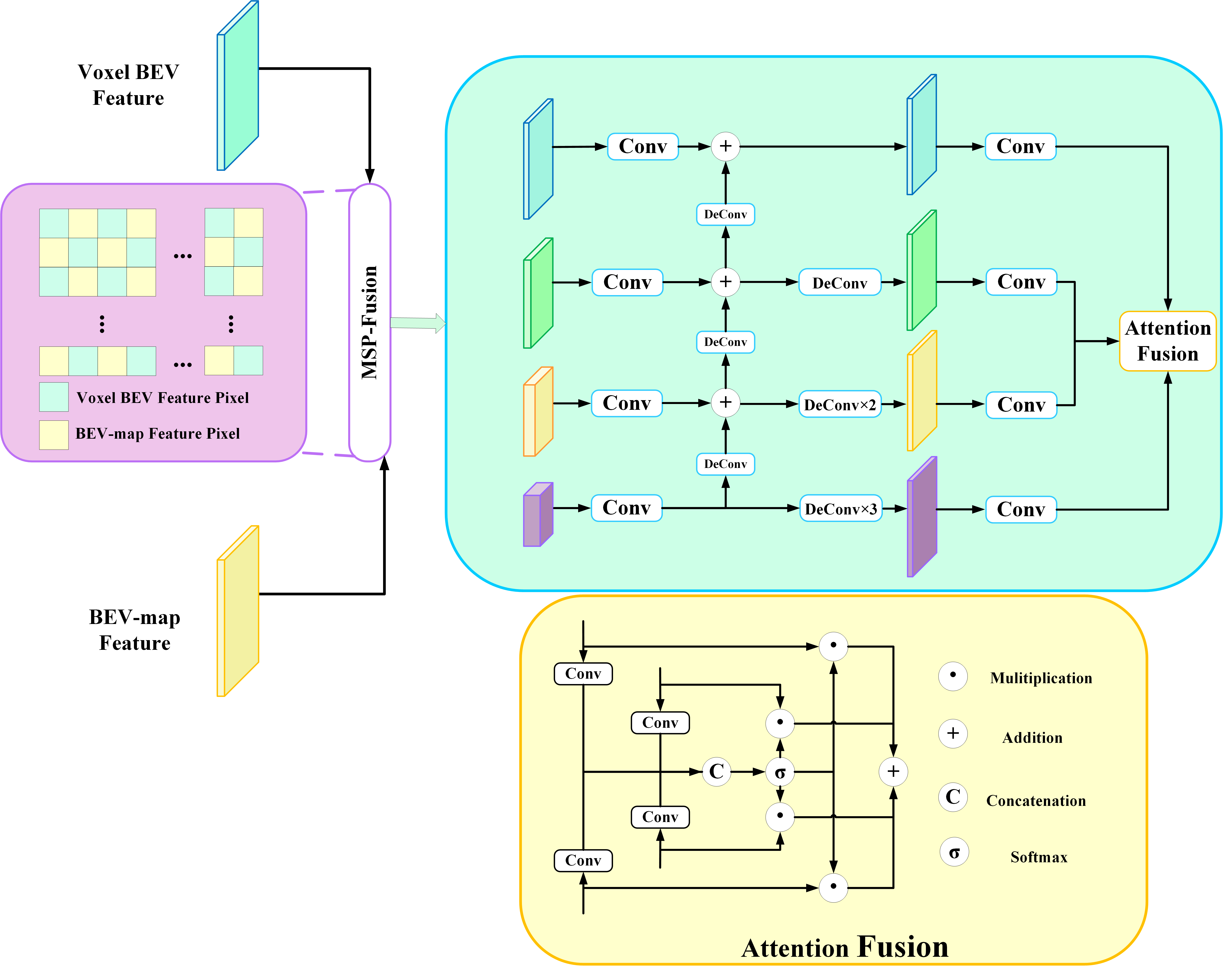
Figure 5: MSSFA network structure. The purple box is the feature fusion part of Voxel-BEV features and BEV-map features; the blue box is the adjustment part for adjusting the feature map size and feature number; the yellow box is the attention fusion module.

III-D Neck

In order to detect cars in autonomous driving, it is necessary to regress each car’s precise location and classify the bounding box of each regression as positive or negative samples. In such a process, it is crucial to consider both low-level spatial features and high-level abstract semantic features. However, when we enrich the high-level abstract semantic features in the feature map by stacking convolutional layers, the resolution of the feature map gradually decreases, resulting in the loss of spatial information in the high-level feature map. In contrast, the low-level features retain more spatial information but contain less abstract semantic features. In CIA-SSD [31], the SSFA module is proposed for fusing feature information at different levels. In this paper, we improve the SSFA module by 1) propose a multi-modal spatial feature fusion solution called MSP-Fusion; 2) using more features with different resolutions as input. We refer to the improved SSFA module as Multi-modal Spatial-Semantic Feature Aggregation module (MSSFA). The structure of MSSFA is shown in Fig. 5.

In the MSP-Fusion module, we perform feature fusion on two modal features with the same positional index and their neighboring features. The structure of MSP-Fusion is illustrated in the purple box in Fig. 5. Firstly, we transform the voxel feature into $((C\times D^{{}^{\prime}}),H^{{}^{\prime}},W^{{}^{\prime}})$ 3D tensor form. Then the number of features is adjusted to be the same as the BEV-map feature in this stage by a $1\times 1$ convolution operation (with $C^{{}^{\prime}}$ denoting the adjusted number of features). Then we will create a $((C^{{}^{\prime}},2H^{{}^{\prime}},2W^{{}^{\prime}})$ tensor, perform adjacent interpolation operations on Voxel-BEV features with the same index and BEV-map features and complete the feature fusion in the Neck part by one $3\times 3$ and one $1\times 1$ convolution operations. The $3\times 3$ convolution allows for the integration of multimodal features in neighboring locations, while the $1\times 1$ convolution allows for further separate feature integration for features at each location of the feature map. In this paper, we use four resolution features as inputs ($304\times 304$, $152\times 152$, $76\times 76$, $38\times 38$). To further demonstrate the effectiveness of MSP-Fusion, in the subsequent ablation experiments, we compared MSP-Fusion proposed in this paper with two other fusion strategies: concatenating features of the two modalities along the feature dimension and directly adding features of the two modalities.

III-E Detection Head and Loss function

In this paper, we use the same detection head as PointPillars, with single shot detector (SSD) [46] settings for 3D object detection. We match the prior boxes to the ground truth using 2D Intersection over Union (IoU) [47]. Bounding box height and elevation were not used for matching; instead given a 2D match, the height and elevation become additional regression targets.

The loss function we use the same loss function as SECOND [29] and PointPillars [26]. Ground truth boxes and anchors are defined by $(x,y,z,w,l,h,\theta)$. The localization regression residuals between ground truth boxes and anchors are defined as (5).

$$\bigtriangleup x=\frac{x^{gt}-x^{a}}{d^{a}},\bigtriangleup y=\frac{y^{gt}-y^{a}}{d^{a}},\bigtriangleup z=\frac{z^{gt}-z^{a}}{d^{a}}\\ \bigtriangleup w=log\frac{w^{gt}}{w^{a}},\bigtriangleup l=log\frac{l^{gt}}{l^{a}},h=\bigtriangleup log\frac{h^{gt}}{h^{a}}$$ (5)

Where $x^{gt}$, $x^{a}$ denote ground truth and anchor boxes, respectively; $d^{a}=\sqrt{(w^{a})^{2}+(l^{a})^{2}}$. The total localization loss can then be defined as:

$$L_{loc}=\sum_{b\in(x,y,z,w,h,l)}SmoothL1(\bigtriangleup b)$$ (6)

We choose Focal loss [48] as the loss function for object classification. Where $\theta_{t}$ is the true value of the object orientation angle and $\theta_{gt}$ is the predicted value of the object orientation angle.

$$L_{cls}=-\theta_{t}log(\theta_{gt})-(1-\theta_{t})log(1-\theta_{gt})$$ (7)

We choose Cross Entropy loss as the regression loss function for the object orientation angle.

$$L_{cls}=-\alpha_{a}(1-p^{\alpha})^{\gamma}log(p^{\alpha})$$ (8)

Where $p^{\alpha}$ is the category probability of an anchor box. We use the parameter settings of $\alpha=0.25$ and $\gamma=2$ from the original paper. Thus, the total loss is as shown in (9). Where $N_{pos}$ represents the number of positive samples, while $\beta_{loc}=2$,$\beta_{cls}=1$,$\beta_{dir}=0.2$.

$$L=\frac{1}{N_{pos}}(\beta_{loc}L_{loc}+\beta_{dir}L_{dir}+\beta_{cls}L_{cls})$$ (9)

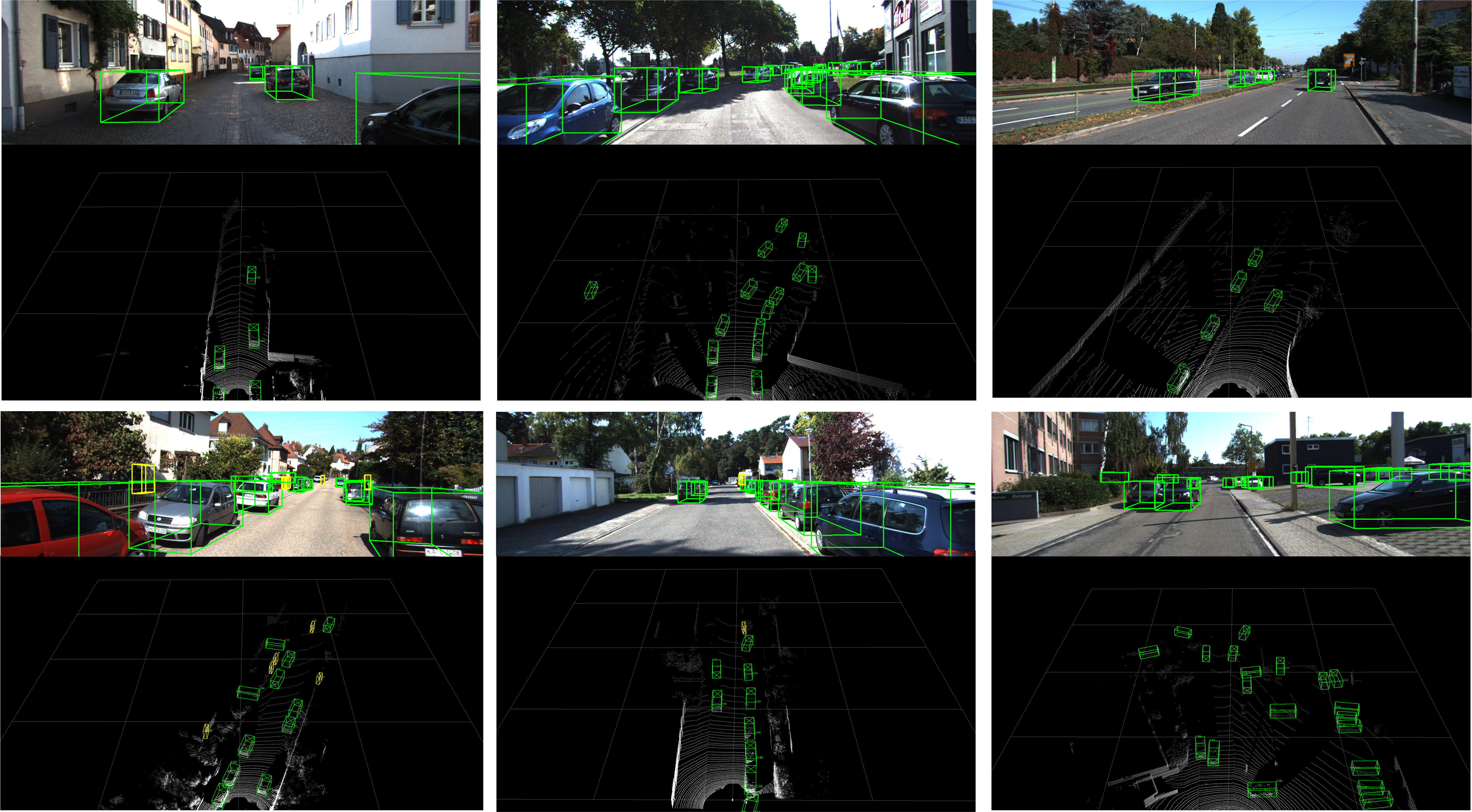
Figure 6: Qualitative analysis of KITTI results. The bottom half is the 3D bounding boxes on the point cloud. The upper part is the 3D bounding box projected into the image for a clearer view. Note that our method uses only LiDAR. We show the predicted boxes for ‘Car’ class (green) and ‘Cyclist’ class (yellow).

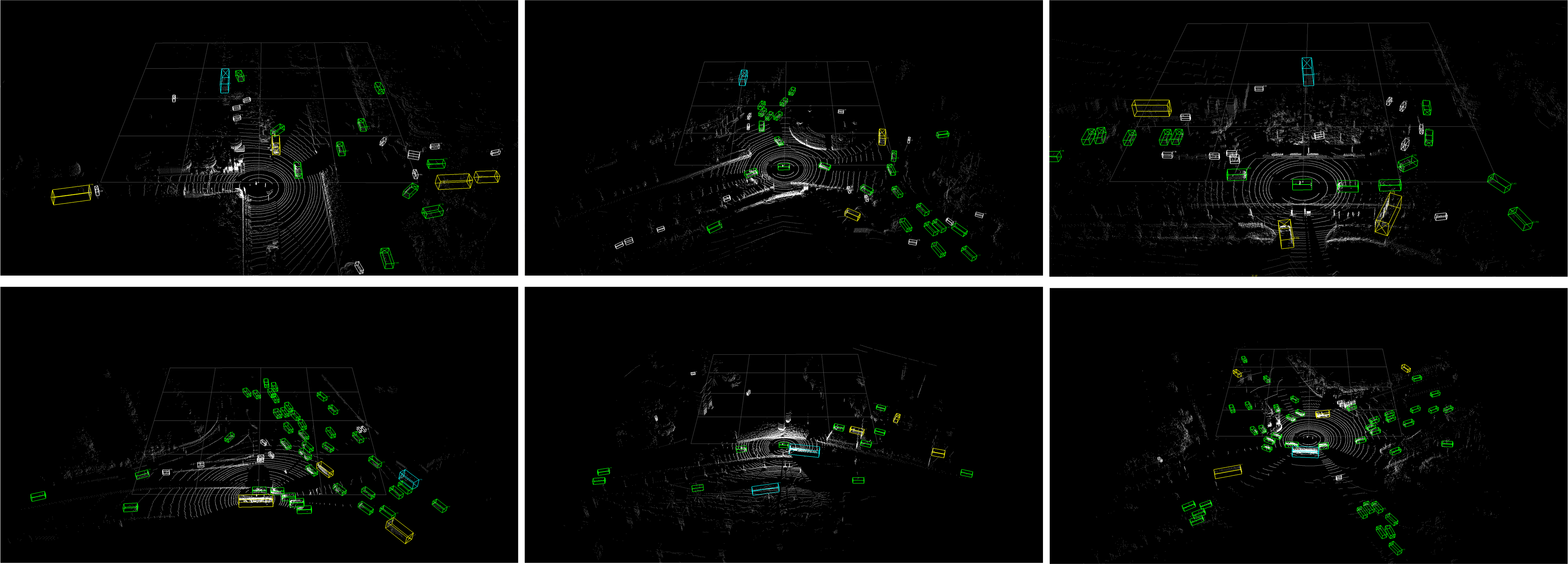
Figure 7: Qualitative analysis of ONCE results. Yellow boxes represent ‘Truck’, green boxes represent ‘Car’, blue boxes represent ‘Bus’, and white boxes represent ‘Cyclist’.

TABLE I: THE 3D DETECTION RESULTS ON THE KITTI TEST SET FOR CAR AND CYCLIST CLASSES USING AP@R40.“L” and “R” represent using LiDAR and RGB images respectively. NOTE THAT WE ONLY COMPARED WITH THE 3D DETECTION PART OF DIFI.

Method	Input	Car $AP_{Bev}$(%)			Cyclist $AP_{Bev}$(%)			Car $AP_{3D}$(%)			Cyclist $AP_{3D}$(%)
		Easy	Mod.	Hard	Easy	Mod.	Hard	Easy	Mod.	Hard	Easy	Mod.	Hard
MV3D[41]	L+I	86.02	76.90	68.49	N/A	N/A	N/A	71.09	62.35	55.12	N/A	N/A	N/A
Cont-Fuse[49]	L+I	88.81	85.83	77.33	N/A	N/A	N/A	82.54	66.22	64.04	N/A	N/A	N/A
Roarnet[50]	L+I	88.20	79.41	70.02	N/A	N/A	N/A	83.71	73.04	59.16	N/A	N/A	N/A
DIFI[51]	L+I	91.01	87.51	84.25	N/A	N/A	N/A	85.29	76.59	71.75	N/A	N/A	N/A
AVOD[40]	L+I	88.53	83.79	77.90	68.09	57.48	50.77	81.84	71.88	66.38	64.00	52.18	46.61
F-PoinNet[18]	L+I	88.70	84.00	75.33	75.38	61.96	54.68	81.20	70.39	62.19	71.69	56.77	50.9
MSL3D[51]	L+I	N/A	N/A	N/A	N/A	N/A	N/A	87.27	81.15	76.56	76.74	62.27	56.20
SMS-Net[33]	L	N/A	N/A	N/A	N/A	N/A	N/A	87.01	76.21	70.45	75.35	60.23	53.37
CIA-SSD[31]	L	N/A	N/A	N/A	N/A	N/A	N/A	89.59	80.28	72.89	N/A	N/A	N/A
Fast Point-RCNN[52]	L	90.87	87.84	80.52	68.09	57.48	50.77	85.29	77.40	70.24	N/A	N/A	N/A
SA-SSD[37]	L	95.03	91.03	85.96	75.38	61.96	54.68	88.75	79.79	74.16	N/A	N/A	N/A
Part-A2[36]	L	91.70	87.79	84.61	83.43	68.73	61.85	87.81	78.49	73.51	79.17	63.52	56.93
PV-RCNN[30]	L	94.98	90.65	86.14	82.49	68.89	62.41	90.25	81.43	76.82	78.60	63.71	57.65
PointRCNN[22]	L	92.13	87.39	82.72	82.56	67.24	60.28	86.96	75.64	70.70	74.96	58.82	52.53
STD[23]	L	94.74	89.19	86.42	81.36	67.23	59.35	87.95	79.91	75.09	78.69	61.59	55.30
SECOND[29]	L	88.07	79.37	77.95	73.67	56.04	48.78	83.13	73.66	66.20	70.51	53.85	46.90
PointPillars[26]	L	88.35	86.10	79.83	79.14	62.25	56.00	79.05	74.99	68.30	75.78	59.07	52.92
H23D R-CNN[32]	L	82.85	88.87	86.07	82.76	67.90	60.49	90.43	81.55	77.22	78.67	62.74	55.78
DVFENet[39]	L	90.93	87.68	84.60	82.29	67.40	60.71	86.20	79.18	74.58	78.73	62.00	55.18
SARPNET[38]	L	88.93	87.26	78.68	79.94	62.80	55.86	84.92	75.64	67.70	77.66	60.43	54.03
Ours	L	91.32	87.46	84.38	81.58	66.93	60.21	86.71	78.53	74.09	78.84	63.00	55.85

TABLE II: THE 3D DETECTION RESULTS ON THE KITTI Val SET FOR CAR AND CYCLIST CLASSES USING AP@R40. “L” and “R” represent using LiDAR and RGB images respectively. NOTE THAT WE ONLY COMPARED WITH THE 3D DETECTION PART OF DIFI.

Method	Modality	Car $AP_{Bev}$(%)			Cyclist $AP_{Bev}$(%)			Car $AP_{3D}$(%)			Cyclist $AP_{3D}$(%)
		Easy	Mod.	Hard	Easy	Mod.	Hard	Easy	Mod.	Hard	Easy	Mod.	Hard
Complex-YOLO[24]	Lidar	85.89	77.40	77.33	72.37	63.36	60.27	67.72	64.00	63.01	68.17	58.32	54.30
Ours	Lidar	90.11	87.93	85.28	82.35	72.18	67.29	88.53	77.80	75.82	84.73	70.17	66.33

TABLE III: Results on the ONCE validation set.

Method	Vehicle				Cyclist				mAP
	$overall$	$0-30m$	$30-50m$	$>50m$	$overall$	$0-30m$	$30-50m$	$>50m$
PV-RCNN[30]	77.77	89.39	72.55	58.64	59.37	71.66	52.58	36.17	68.57
Point RCNN[22]	52.09	74.45	40.89	16.81	29.84	46.03	20.94	5.46	40.97
PointPillars[26]	68.57	80.86	62.07	47.04	46.81	58.33	40.32	25.86	57.69
CenterPoints[53]	66.79	80.10	59.55	43.39	63.45	74.28	57.94	41.48	65.12
SECOND[29]	71.19	84.04	63.02	47.25	58.04	69.69	52.43	34.61	64.62
Ours	69.24	84.14	64.29	42.67	54.06	69.32	44.89	25.18	61.65

TABLE IV: Experimental results of comparison experiments with other algorithms. The detection speed was compared on the GTX1060.

Method	PontRCNN[22]	PV-RCNN[30]	SECOND[29]	PointPillars[26]	PartA2[36]	Ours
FPS	3	3.8	11	15	3	5

TABLE V: PERFORMANCE COMPARISON ON THE KITTI VAL SET, WITH AP CALCULATED BY 11 RECALL POSITIONS FOR CAR AND CYCLIST. BOLDED VALUES ARE THE BEST PERFORMANCES FOR ALL METHODS.

Improved Part		Method A	Method B	Method C	Method D	Method E
BEV		$\surd$		$\surd$	$\surd$	$\surd$
Voxel			$\surd$	$\surd$	$\surd$	$\surd$
PWF-Net					$\surd$	$\surd$
MSSFA		$\surd$	$\surd$	$\surd$	$\surd$	$\surd$
Re-voxelization layer						$\surd$
Re-voxelization layer(Randomly Sample)			$\surd$	$\surd$	$\surd$
Car AP	Easy	80.61	89.36	89.77	89.80	90.11
BEV Detection	Mod.	66.83	87.00	87.80	87.52	87.93
(IoU=0.7)	Hard	64.22	82.55	83.62	82.44	85.28
Cyclist AP	Easy	54.46	78.03	83.02	83.18	85.35
BEV Detection	Mod.	42.66	64.39	67.20	69.75	72.18
(IoU=0.5)	Hard	41.44	60.41	66.88	65.76	67.29
Car AP	Easy	62.15	85.76	87.61	87.45	88.53
3D Detection	Mod.	52.11	75.96	76.43	76.88	77.80
(IoU=0.7)	Hard	50.00	71.18	72.44	71.44	75.82
Cyclist AP	Easy	44.00	76.37	80.00	82.02	84.73
3D Detection	Mod.	42.12	59.63	66.20	67.65	70.17
(IoU=0.5)	Hard	39.25	57.33	62.15	63.00	66.33

TABLE VI: ANALYSIS OF THE MULTI FEATURES FUSION OPERATION.NOTATION: ‘MSP’ REPRESENTS MSP-Fusion MODULE. BOLDED VALUES ARE THE BEST PERFORMANCES FOR ALL METHODS.

Method	Feature Fusion				Mod. AP${}_{3D}(\%)$
	BEV	Voxel	MSP	Concat	Car	Cyclist
A	$\surd$				52.11	42.12
B		$\surd$			75.96	59.63
F	$\surd$	$\surd$		$\surd$	75.49	62.29
C	$\surd$	$\surd$	$\surd$		76.43	66.20

IV Experiments and Results

IV-A Datasets

We evaluated our method on the KITTI 3D object benchmark dataset [54]. The KITTI dataset has 7,481 training samples and 7,518 test samples. The training samples were divided into a training set (3,712 samples) and a validation set (3,769 samples). We conducted experiments on the most commonly used ‘Car’ and ‘Cyclist’ classes and evaluated the results by average precision (AP) and IoU thresholds (0.7 for cars and 0.5 for bicycles). Also, the dataset has three difficulty levels (easy, medium, and hard) based on object size, occlusion, and truncation levels. Fig. 6 shows the results of our predictions.

To further validate the effectiveness of our algorithm, we evaluated the performance of our algorithm on the ONCE dataset [55]. Six sequences were used for training, and four sequences were used for validation. We trained our method on the training set and evaluated it on the validation set. The ONCE dataset is divided into four evaluation levels based on the distance of objects (overall, objects within 0-30m range, objects within 30-50m range, objects beyond 50m range), and the evaluation metrics include Average Precision (AP) and Mean Average Precision (mAP). Fig. 7 shows the results of our predictions.

IV-B Implementation Details

For KITTI dataset, we project the point cloud data in the range of $[0m,60.8m]$, $[-30.4m,30.4m]$. The point cloud data in the range of $[-3m,1m]$ (along the x-axis, y-axis, and z-axis) is projected to the bird’s-eye view to construct a $608\times 608$ BEV-map with each pixel corresponding to a realistic size of $[0.1m,0.1m$]. The size of each voxel after voxelization is $[0.1m,0.1,0m.125m]$, and the number of point clouds is 12. For ONCE dataset, we project the point cloud data in the range of $[-60.8m,60.8m]$, $[-60.8m,60.8m]$. The point cloud data in the range of $[-5m,3m]$ (along the x-axis, y-axis, and z-axis) is projected to the bird’s-eye view to construct a $608\times 608$ BEV-map with each pixel corresponding to a realistic size of $[0.2m,0.2m$]. The size of each voxel after voxelization is $[0.2m,0.2,0m.25m]$, and the number of point clouds is 12.

For the data augmentation part, we first created a look-up table of ground truth 3D boxes for all categories and the associated point clouds that fall within these 3D boxes, following the approach of SECOND [29]. Then, for each sample, we randomly selected 15 ground truth samples for ‘Car’ class and 15 for ‘Cyclist’ class, respectively, and placed them into the current point cloud. Next, these ground truth boxes are individually augmented with data. Each ground truth box was randomly rotated (drawn from $[-\pi/4,\pi/4]$) and translated (x, y, and z values were randomly drawn from $[0,0.5]$). Finally, two sets of global data augmentation are performed, a random mirror flip along the x-axis [56] and a global scaling [29, 28] (scaling is randomly drawn from $[0.95,1.05]$). Please refer to OpenPCDet for the specific configuration. We implemented the method of this paper using OpenPCDet and completed all the experiments.

For the feature extraction network of BEV-map we have chosen ConvNeXt-Tiny [42]. The voxel feature extraction network is stacked by VR-VFE layer. In the MSSFA module, we take the outputs of Stage1, Stage2, Stage3, and Stage4 of the feature voxel extraction network as its input (corresponding to resolutions of $152\times 152$, $76\times 76$, $38\times 38$, $19\times 19$). The BEV-map feature and Voxel BEV feature of the same stage perform adjacent interpolation operations. Then the output is adjusted for the number of channels with a $1\times 1$ convolution with 256 output channels, and the features are fused with a $3\times 3$ convolution with stride of 1 and padding of 1. The 2D DeConv layer consists of a $3\times 3$ convolution and a $3\times 3$ deconvolution. In attention fusion, a $3\times 3$ convolution is performed with an output channel of 1 to obtain the attention map. The head network settings obey the settings in PointPillars [26].

We merged the validation set of the KITTI dataset with the training set to construct a new training set (3,712 samples in the original training set and 3,769 samples in the original validation set, with a total of 7,481 samples in the combined training set). The ADAM optimizer [57] and OnecycleLR [58] were applied to train 100 epochs with the initial learning rate set to 0.003, weight decay to 0.01, and momentum to 0.9.

IV-C Compared with Others

All detection results were measured using the official KITTI evaluation detection metrics of bird’s eye view (BEV), 3D, 2D, and average orientation similarity (AOS). 2D detection was performed in the image plane; AOS evaluates the average direction of 2D detection (measured by BEV, IoU threshold of 0.7 for ‘Car’ class and 0.5 for ‘Cyclist’ class). The experimental results are shown in Table i@ and ii@.

Table i@ shows the 3D detection AP and BEV detection AP of our method on the KITTI test set. In both tables, we classify these methods into two categories based on the type of sensor used (methods such as MV3D use both camera and Lidar, while methods such as PV-RCNN use Lidar). From the table, we can see that our method’s AP for ’Car’ class performs poorly, with 3D AP of 86.71%, 78.53%, and 74.09% under Easy, Mod, and Hard conditions, respectively, which has a certain gap with advanced methods such as PV-RCNN. However, compared with projection-based 3D object detection methods[40, 41, 26], our method all have good advantages. For the ’Cyclist’ class AP, our method has good performance. The 3D AP for ‘Cyclist’ class is 78.84%, 63.00%, and 55.85%.

As can be seen from Table i@, our method has 3% lower 3D AP in the ‘Car’ class compared to the H²3D R-CNN[32], which is also based on the projection method. After our analysis, the reasons are: (1) The H23D R-CNN uses a dynamic voxelization feature coding method [59], establishing a complete mapping relationship between points and voxels. In contrast, this paper uses a hard voxelization approach [28], which leads to uncertain voxel filling and information loss due to random sampling and discarding operations. (2) The projected features in the H23D R-CNN retain higher dimensional feature information through the MLP layer. In contrast, this paper uses the same feature coding method as Complex-YOLO [24], which over-compresses the features in the bird’s-eye view, resulting in information loss. (3) H23D R-CNN is a two-stage 3D detector that fully uses the prior knowledge of the Region Proposal Network (RPN) module. In contrast, the method in this paper is a one-stage 3D detector, and the detection accuracy depends heavily on how well the features are extracted. However, we found that our method has good accuracy for objects with fewer reflection points like cyclist. We analyzed the main reasons for this as: (1) However, the hard voxelization we use causes some information loss, we use a weight-based feature point sampling method in the Re-voxelization layer proposed in this paper. For objects with fewer reflective points, such as cyclists, we can prioritize the feature points that are more beneficial to the detection task. (2) PWF-Net can filter out the point feature information more beneficial to the detection task. (3) For objects with few reflection points and small sizes, like the ’Cyclist’ class, the voxel description in 3D space is more responsive to its features than the 2D perspective view. In the MSSFA module, we complemented the BEV-map features with voxel BEV features at the same grid points. In the subsequent ablation experiments, we can also see that the Re-voxelization layer, PWF-Net and the feature fusion module in MSSFA have a good improvement of the detection accuracy for the ’Cyclist’ class.

Table ii@ shows the results of our comparison with Complex-YOLO [24]. Considering that the detection results for the KITTI test set are not submitted in Complex-YOLO, we compared our method with Complex-YOLO on the val set of KITTI. In this paper, the same bird’s-eye view projection encoding method as Complex-YOLO is used. As can be seen in Table ii@, our method is more advantageous in both BEV AP and 3D AP. Although in 3D detection, Complex-YOLO does not predict the height of the object, which affects the accuracy of 3D detection to some extent, our method has a greater improvement compared with it in the BEV detection results.

Table iii@ shows the detection results of the method proposed in this paper on the validation set of the ONCE dataset. From Table iii@, it can be seen that the proposed method performs well in large-scale complex LiDAR scenes. Compared to the projection-based method PointPillars, our method demonstrates a good precision advantage on the ONCE dataset. In Fig. 8, we present the visualized detection results on the ONCE dataset.

To validate the detection speed of our method, we compared it with several other methods on a device equipped with GTX1060. As shown in Table iv@, it is evident that due to the presence of a multi-branch structure, our method does not perform well in terms of detection speed.

IV-D Ablation Experiment

To further validate the validate the effectiveness of each part of our method, we performed further validation on the validation set of the KITTI dataset. All experiments were per-formed on the same data set division (3,712 samples for the training set and 3,769 samples for the validation set), using the same parameter configuration and 100 epochs trained. The experimental results are shown in Table v@. In Table v@, ‘BEV’ and ‘Voxel’ denote BEV-map or voxel as input. ‘Re-Voxelization Layer (Randomly Sample)’ denote the Re-Voxelization Layer with randomly sampling instead of sampling by point weights.

Method A: Method A uses BEV-map as input and ConvNeXt-Tiny for feature extraction. Because only BEV-map is used as is input, the feature fusion part is removed from the MSSFA module that is not available in Method A. The resolution of BEV-map is 608×608, and the used point cloud range is $[60.8m,60.8m,4m]$. The rest of the settings are the same as the method proposed in this paper. As can be seen from Table v@, the detection results obtained by using only BEV-map as input are poor. This is because projecting the point cloud to the bird’s view causes more information loss in the data processing stage, which is not beneficial for the subsequent detection tasks.

Method B: Method B uses voxel as input, and a voxel feature extraction network constructed by stacking SVFE and Re-voxelization (Randomly Sample) layer is used for feature extraction. Because only voxel is used as input, the feature fusion part is removed from the MSSFA module that is not available in Method B. The used point cloud range is $[60.8m,60.8m,4m]$. The size of each voxel is $[0.1m,0.1,0m.125m]$, and each voxel is randomly sampled with 12 points. The rest of the settings are the same as the method proposed in this paper. Compared with Method A, the voxel can retain more point cloud information, and the Re-voxelization layer is designed to achieve feature interaction of adjacent voxels. Compared with Method A, the detection accuracy of Method B is greatly improved.

Method C: Method C uses a mixture of BEV-map and voxel as input. Compared with methods A and B, the fusion of voxel and BEV-map features was added to the MSSFA module. BEV-map and voxel have the same parameters as methods A and B. The rest of the settings are the same as the method proposed in this paper. The detection accuracy has been improved compared to Method A and Method B (compared to Method A, 3D AP of ’Car’ class is improved by 25.46%, 24.32%, 22.44%, 3D AP of ’Cyclist’ class is improved by 36%, 22.08%, 22.9%; compared to Method B, 3D AP of ’Car’ class is improved by 1.85%, 0.47%, 0.56%, 3D AP of ’Cyclist’ class is improved by 3.63%, 6.57%, and 4.82%).

Method D: Method D adds PWF-Net to Method C. The rest of the settings are the same as the method proposed in this paper. Compared to Method C, Method D has improved detection accuracy in ‘Cyclist’ class (compared to Method C, 3D AP of ‘Car’ class is improved by 2.02%, 1.35%, 0.85%, 3D AP of ‘Cyclist’ class is improved by 2.02%, 1.35%, 0.85%).

Method E: Method E (the method proposed in this paper) replaces random sampling with perpoint weight sampling. Compared with Method D, the detection accuracy of Method E is improved more in the detection accuracy of small objects like cyclist with fewer point clouds (compared with Method D, the 3D AP of ‘Car’ is improved by 1.08%, 0.92%, 4.38%, the 3D AP of ‘Cyclist’ class is improved by 4.71%,2.52%, 3.33%).

By comparing Method A and C, we can find that voxel can be used to compensate for the information loss of the point cloud during projection. Compared with Method B, Method C adds point cloud projection as input, which can also help the final detection task. The comparison between Method C, D, and E shows that the PWF-Net and the Re-voxelization layer sampled by weight are good for detecting objects with few reflection points like cyclist. This is because, for objects with fewer points, the Re-voxelization layer with weight sampling and PWF-Net can filter out the feature points that are more beneficial for the detection task.

In the MSSFA module, we added the feature fusion module for Voxel-BEV and BEV-map feature fusion. To verify the effective ness of our feature fusion module design, we designed the corresponding comparison experiments. Table vi@ shows the experimental results. Method A, B, and C, in Table vi@, corresponding to the methods mentioned in Table v@. We modify the feature fusion module in MSSFA to Concat operation (i.e., stitching by feature dimension) in Method F. The rest of the module design in Method F is the same as Method C. As we can see from Table vi@, compared to Method F, Method C has improved 3D AP in Mod. conditions (’Car’:0.94%, ’Cyclist’:3.91%). The 3D AP of ’Car’ and ’Cyclist’ are also improved by Method F under Mod. conditions compared to Method A, B (’Car’: 23% compared to Method A, B, ’Cyclist’: 20.17%, 2.66%; ’Car’ by 23.38%, -0.47%, respectively).

V Conclusion

In this paper, we propose a combined voxel and point cloud projection one-stage end-to-end 3D detector. Our main contributions include: combining voxel with point cloud projection to compensate for the information loss during point cloud projection; proposing a voxel feature extraction network with variable perceptual field;introducing a multimodal spatial feature fusion method based on SSFA; and proposing a feature fusion module for point cloud projection and voxel. Although compared with H23D R-CNN, PV-RCNN, our method has a large gap in the detection of ’Car’ class. However, our method has a good advantage compared to projection-based methods such as AVOD, PointPillars, etc. Also, it proves that the information loss in the projection process can be compensated by adding voxel feature encoding. In addition, our proposed Re-Voxelization Layer and PWF-Net can better utilize fewer points for the detection task of objects with fewer reflection points, such as the ’Cyclist’ class. Although our method shows a notable improvement in detection accuracy compared to methods like PointPillars, the detection speed is compromised due to the multi-branch feature extraction structure. In future work, we can explore using a relatively lightweight BEV-map feature extraction network and further optimize the voxel feature extraction network.

References

- [1] W. Zhou, S. Pan, J. Lei, and L. Yu, “Tmfnet: Three-input multilevel fusion network for detecting salient objects in rgb-d images,” IEEE Transactions on Emerging Topics in Computational Intelligence, vol. 6, no. 3, pp. 593–601, 2021.
- [2] R. Barkur, D. Suresh, S. Lal, C. S. Reddy, P. Diwakar et al., “Rscdnet: A robust deep learning architecture for change detection from bi-temporal high resolution remote sensing images,” IEEE Transactions on Emerging Topics in Computational Intelligence, vol. 7, no. 2, pp. 537–551, 2022.
- [3] R. Cong, W. Song, J. Lei, G. Yue, Y. Zhao, and S. Kwong, “Psnet: Parallel symmetric network for video salient object detection,” IEEE Transactions on Emerging Topics in Computational Intelligence, vol. 7, no. 2, pp. 402–414, 2022.
- [4] Y. Li, C. Pan, X. Cao, and D. Wu, “Power line detection by pyramidal patch classification,” IEEE Transactions on Emerging Topics in Computational Intelligence, vol. 3, no. 6, pp. 416–426, 2018.
- [5] L. Chen, X. Jiang, X. Liu, T. Kirubarajan, and Z. Zhou, “Outlier-robust moving object and background decomposition via structured -regularized low-rank representation,” IEEE Transactions on Emerging Topics in Computational Intelligence, vol. 5, no. 4, pp. 620–638, Aug 2021.
- [6] J. Chen, H. Chen, Y. Guo, M. Zhou, R. Huang, and C. Mao, “A novel test case generation approach for adaptive random testing of object-oriented software using k-means clustering technique,” IEEE Transactions on Emerging Topics in Computational Intelligence, vol. 6, no. 4, pp. 969–981, 2021.
- [7] A. Pramanik, S. K. Pal, J. Maiti, and P. Mitra, “Granulated rcnn and multi-class deep sort for multi-object detection and tracking,” IEEE Transactions on Emerging Topics in Computational Intelligence, vol. 6, no. 1, pp. 171–181, 2021.
- [8] H. Wang, Y. Xu, Z. Wang, Y. Cai, L. Chen, and Y. Li, “Centernet-auto: A multi-object visual detection algorithm for autonomous driving scenes based on improved centernet,” IEEE Transactions on Emerging Topics in Computational Intelligence, 2023.
- [9] W. Zhou, Y. Zhu, J. Lei, J. Wan, and L. Yu, “Apnet: Adversarial learning assistance and perceived importance fusion network for all-day rgb-t salient object detection,” IEEE Transactions on Emerging Topics in Computational Intelligence, vol. 6, no. 4, pp. 957–968, 2021.
- [10] X. Chen, K. Kundu, Y. Zhu, A. G. Berneshawi, H. Ma, S. Fidler, and R. Urtasun, “3d object proposals for accurate object class detection,” Advances in neural information processing systems, vol. 28, 2015.
- [11] Z. Deng and L. Jan Latecki, “Amodal detection of 3d objects: Inferring 3d bounding boxes from 2d ones in rgb-depth images,” in Proceedings of the IEEE Conference on Computer Vision and Pattern Recognition, 2017, pp. 5762–5770.
- [12] D. Xu, W. Ouyang, E. Ricci, X. Wang, and N. Sebe, “Learning cross-modal deep representations for robust pedestrian detection,” in Proceedings of the IEEE conference on computer vision and pattern recognition, 2017, pp. 5363–5371.
- [13] S. Gupta, R. Girshick, P. Arbeláez, and J. Malik, “Learning rich features from rgb-d images for object detection and segmentation,” in Computer Vision–ECCV 2014: 13th European Conference, Zurich, Switzerland, September 6-12, 2014, Proceedings, Part VII 13. Springer, 2014, pp. 345–360.
- [14] Y. Chen, S. Liu, X. Shen, and J. Jia, “Dsgn: deep stereo geometry network for 3d object detection, 2020 ieee,” in CVF conference on computer vision and pattern recognition (CVPR), 2020, pp. 12 533–12 542.
- [15] J.-R. Chang and Y.-S. Chen, “Pyramid stereo matching network,” in Proceedings of the IEEE conference on computer vision and pattern recognition, 2018, pp. 5410–5418.
- [16] P. Li, X. Chen, and S. Shen, “Stereo r-cnn based 3d object detection for autonomous driving,” in Proceedings of the IEEE/CVF Conference on Computer Vision and Pattern Recognition, 2019, pp. 7644–7652.
- [17] C. Nie, Z. Ju, Z. Sun, and H. Zhang, “3d object detection and tracking based on lidar-camera fusion and imm-ukf algorithm towards highway driving,” IEEE Transactions on Emerging Topics in Computational Intelligence, 2023.
- [18] C. R. Qi, W. Liu, C. Wu, H. Su, and L. J. Guibas, “Frustum pointnets for 3d object detection from rgb-d data,” in Proceedings of the IEEE conference on computer vision and pattern recognition, 2018, pp. 918–927.
- [19] C. R. Qi, H. Su, K. Mo, and L. J. Guibas, “Pointnet: Deep learning on point sets for 3d classification and segmentation,” in Proceedings of the IEEE conference on computer vision and pattern recognition, 2017, pp. 652–660.
- [20] C. R. Qi, L. Yi, H. Su, and L. J. Guibas, “Pointnet++: Deep hierarchical feature learning on point sets in a metric space,” Advances in neural information processing systems, vol. 30, 2017.
- [21] T. Guan, J. Wang, S. Lan, R. Chandra, Z. Wu, L. Davis, and D. Manocha, “M3detr: Multi-representation, multi-scale, mutual-relation 3d object detection with transformers,” in Proceedings of the IEEE/CVF Winter Conference on Applications of Computer Vision (WACV), January 2022, pp. 772–782.
- [22] S. Shi, X. Wang, and H. Li, “Pointrcnn: 3d object proposal generation and detection from point cloud,” in Proceedings of the IEEE/CVF conference on computer vision and pattern recognition, 2019, pp. 770–779.
- [23] Z. Yang, Y. Sun, S. Liu, X. Shen, and J. Jia, “Std: Sparse-to-dense 3d object detector for point cloud,” in Proceedings of the IEEE/CVF international conference on computer vision, 2019, pp. 1951–1960.
- [24] M. Simony, S. Milzy, K. Amendey, and H.-M. Gross, “Complex-yolo: An euler-region-proposal for real-time 3d object detection on point clouds,” in Proceedings of the European conference on computer vision (ECCV) workshops, 2018, pp. 0–0.
- [25] Y. Shao, Z. Sun, A. Tan, and T. Yan, “Efficient three-dimensional point cloud object detection based on improved complex-yolo,” Frontiers in Neurorobotics, vol. 17, p. 1092564, 2023.
- [26] A. H. Lang, S. Vora, H. Caesar, L. Zhou, J. Yang, and O. Beijbom, “Pointpillars: Fast encoders for object detection from point clouds,” in Proceedings of the IEEE/CVF conference on computer vision and pattern recognition, 2019, pp. 12 697–12 705.
- [27] W. Ali, S. Abdelkarim, M. Zidan, M. Zahran, and A. El Sallab, “Yolo3d: End-to-end real-time 3d oriented object bounding box detection from lidar point cloud,” in Proceedings of the European conference on computer vision (ECCV) workshops, 2018, pp. 0–0.
- [28] Y. Zhou and O. Tuzel, “Voxelnet: End-to-end learning for point cloud based 3d object detection,” in Proceedings of the IEEE conference on computer vision and pattern recognition, 2018, pp. 4490–4499.
- [29] Y. Yan, Y. Mao, and B. Li, “Second: Sparsely embedded convolutional detection,” Sensors, vol. 18, no. 10, p. 3337, 2018.
- [30] S. Shi, C. Guo, L. Jiang, Z. Wang, J. Shi, X. Wang, and H. Li, “Pv-rcnn: Point-voxel feature set abstraction for 3d object detection,” in Proceedings of the IEEE/CVF conference on computer vision and pattern recognition, 2020, pp. 10 529–10 538.
- [31] W. Zheng, W. Tang, S. Chen, L. Jiang, and C.-W. Fu, “Cia-ssd: Confident iou-aware single-stage object detector from point cloud,” in Proceedings of the AAAI conference on artificial intelligence, vol. 35, no. 4, 2021, pp. 3555–3562.
- [32] J. Deng, W. Zhou, Y. Zhang, and H. Li, “From multi-view to hollow-3d: Hallucinated hollow-3d r-cnn for 3d object detection,” IEEE Transactions on Circuits and Systems for Video Technology, vol. 31, no. 12, pp. 4722–4734, 2021.
- [33] S. Liu, W. Huang, Y. Cao, D. Li, and S. Chen, “Sms-net: Sparse multi-scale voxel feature aggregation network for lidar-based 3d object detection,” Neurocomputing, vol. 501, pp. 555–565, 2022.
- [34] W. Xu, L. Zou, Z. Fu, L. Wu, and Y. Qi, “Two-stage 3d object detection guided by position encoding,” Neurocomputing, vol. 501, pp. 811–821, 2022.
- [35] J. Deng, S. Shi, P. Li, W. Zhou, Y. Zhang, and H. Li, “Voxel r-cnn: Towards high performance voxel-based 3d object detection,” in Proceedings of the AAAI Conference on Artificial Intelligence, vol. 35, no. 2, 2021, pp. 1201–1209.
- [36] S. Shi, Z. Wang, J. Shi, X. Wang, and H. Li, “From points to parts: 3d object detection from point cloud with part-aware and part-aggregation network,” IEEE transactions on pattern analysis and machine intelligence, vol. 43, no. 8, pp. 2647–2664, 2020.
- [37] C. He, H. Zeng, J. Huang, X.-S. Hua, and L. Zhang, “Structure aware single-stage 3d object detection from point cloud,” in Proceedings of the IEEE/CVF conference on computer vision and pattern recognition, 2020, pp. 11 873–11 882.
- [38] Y. Ye, H. Chen, C. Zhang, X. Hao, and Z. Zhang, “Sarpnet: Shape attention regional proposal network for lidar-based 3d object detection,” Neurocomputing, vol. 379, pp. 53–63, 2020.
- [39] Y. He, G. Xia, Y. Luo, L. Su, Z. Zhang, W. Li, and P. Wang, “Dvfenet: Dual-branch voxel feature extraction network for 3d object detection,” Neurocomputing, vol. 459, pp. 201–211, 2021.
- [40] J. Ku, M. Mozifian, J. Lee, A. Harakeh, and S. L. Waslander, “Joint 3d proposal generation and object detection from view aggregation,” in 2018 IEEE/RSJ International Conference on Intelligent Robots and Systems (IROS). IEEE, 2018, pp. 1–8.
- [41] X. Chen, H. Ma, J. Wan, B. Li, and T. Xia, “Multi-view 3d object detection network for autonomous driving,” in Proceedings of the IEEE conference on Computer Vision and Pattern Recognition, 2017, pp. 1907–1915.
- [42] Z. Liu, H. Mao, C.-Y. Wu, C. Feichtenhofer, T. Darrell, and S. Xie, “A convnet for the 2020s,” in Proceedings of the IEEE/CVF conference on computer vision and pattern recognition, 2022, pp. 11 976–11 986.
- [43] K. He, X. Zhang, S. Ren, and J. Sun, “Deep residual learning for image recognition,” in Proceedings of the IEEE conference on computer vision and pattern recognition, 2016, pp. 770–778.
- [44] A. Dosovitskiy, L. Beyer, A. Kolesnikov, D. Weissenborn, X. Zhai, T. Unterthiner, M. Dehghani, M. Minderer, G. Heigold, S. Gelly et al., “An image is worth 16x16 words: Transformers for image recognition at scale,” arXiv preprint arXiv:2010.11929, 2020.
- [45] Z. Liu, Y. Lin, Y. Cao, H. Hu, Y. Wei, Z. Zhang, S. Lin, and B. Guo, “Swin transformer: Hierarchical vision transformer using shifted windows,” in Proceedings of the IEEE/CVF international conference on computer vision, 2021, pp. 10 012–10 022.
- [46] W. Liu, D. Anguelov, D. Erhan, C. Szegedy, S. Reed, C.-Y. Fu, and A. C. Berg, “Ssd: Single shot multibox detector,” in Computer Vision–ECCV 2016: 14th European Conference, Amsterdam, The Netherlands, October 11–14, 2016, Proceedings, Part I 14. Springer, 2016, pp. 21–37.
- [47] M. Everingham, L. Van Gool, C. K. Williams, J. Winn, and A. Zisserman, “The pascal visual object classes (voc) challenge,” International journal of computer vision, vol. 88, pp. 303–338, 2010.
- [48] T.-Y. Lin, P. Goyal, R. Girshick, K. He, and P. Dollár, “Focal loss for dense object detection,” in Proceedings of the IEEE international conference on computer vision, 2017, pp. 2980–2988.
- [49] M. Liang, B. Yang, S. Wang, and R. Urtasun, “Deep continuous fusion for multi-sensor 3d object detection,” in Proceedings of the European conference on computer vision (ECCV), 2018, pp. 641–656.
- [50] K. Shin, Y. P. Kwon, and M. Tomizuka, “Roarnet: A robust 3d object detection based on region approximation refinement,” in 2019 IEEE intelligent vehicles symposium (IV). IEEE, 2019, pp. 2510–2515.
- [51] W. Chen, P. Li, and H. Zhao, “Msl3d: 3d object detection from monocular, stereo and point cloud for autonomous driving,” Neurocomputing, vol. 494, pp. 23–32, 2022.
- [52] Y. Chen, S. Liu, X. Shen, and J. Jia, “Fast point r-cnn,” in Proceedings of the IEEE/CVF international conference on computer vision, 2019, pp. 9775–9784.
- [53] T. Yin, X. Zhou, and P. Krahenbuhl, “Center-based 3d object detection and tracking,” in Proceedings of the IEEE/CVF conference on computer vision and pattern recognition, 2021, pp. 11 784–11 793.
- [54] A. Geiger, P. Lenz, and R. Urtasun, “Are we ready for autonomous driving? the kitti vision benchmark suite,” in 2012 IEEE conference on computer vision and pattern recognition. IEEE, 2012, pp. 3354–3361.
- [55] J. Mao, M. Niu, C. Jiang, H. Liang, J. Chen, X. Liang, Y. Li, C. Ye, W. Zhang, Z. Li et al., “One million scenes for autonomous driving: Once dataset,” arXiv preprint arXiv:2106.11037, 2021.
- [56] B. Yang, W. Luo, and R. Urtasun, “Pixor: Real-time 3d object detection from point clouds,” in Proceedings of the IEEE conference on Computer Vision and Pattern Recognition, 2018, pp. 7652–7660.
- [57] D. P. Kingma and J. Ba, “Adam: A method for stochastic optimization,” arXiv preprint arXiv:1412.6980, 2014.
- [58] L. N. Smith and N. Topin, “Super-convergence: Very fast training of neural networks using large learning rates,” in Artificial intelligence and machine learning for multi-domain operations applications, vol. 11006. SPIE, 2019, pp. 369–386.
- [59] Y. Zhou, P. Sun, Y. Zhang, D. Anguelov, J. Gao, T. Ouyang, J. Guo, J. Ngiam, and V. Vasudevan, “End-to-end multi-view fusion for 3d object detection in lidar point clouds,” in Conference on Robot Learning. PMLR, 2020, pp. 923–932.