High Temperature Superconductivity in La₃Ni₂O₇

Abstract

Motivated by the recent discovery of high-temperature superconductivity in bilayer La₃Ni₂O₇ under pressure, we study its electronic properties and superconductivity due to strong electron correlation. Using the inversion symmetry, we decouple the low-energy electronic structure into block-diagonal symmetric and antisymmetric sectors. We find that the antisymmetric sector can be reduced to a one-band system near half filling, while the symmetric bands occupied by about two electrons are heavily overdoped individually. Using the strong coupling mean field theory, we obtain strong superconducting pairing with $B_{1g}$ symmetry in the antisymmetric sector. We propose that due to the spin-orbital exchange coupling between the two sectors, $B_{1g}$ pairing is induced in the symmetric bands, which in-turn boosts the pairing gap in the antisymmetric band and enhances the high-temperature superconductivity with a congruent $d$-wave symmetry in pressurized La₃Ni₂O₇.

The discovery of high-temperature (high-T_c) superconductivity in the cuprates Bednorz and Müller (1986), whose transition temperatures greatly exceed conventional superconductors, encourages exploring none-copper-based high-T_c superconductors both experimentally and theoretically Lee et al. (2006); Keimer et al. (2015); Maeno et al. (1994); Kamihara et al. (2008); Takahashi et al. (2008); Paglione and Greene (2010); Hu et al. (2015). Among this exploration, it was theoretically proposed that the nickelates could be a counterpart of the cuprates Anisimov et al. (1999); Lee and Pickett (2004). Owing to sustained efforts on the synthesis Crespin et al. (1983a); Greenblatt (1997); Hayward et al. (1999); Crespin et al. (1983b, 2005); Kawai et al. (2010), superconductivity was finally found in the “infinite-layer” nickelates (Sr,Nd) NiO₂ thin films Li et al. (2019); Osada et al. (2020); Li et al. (2020), opening the Nickel age of superconductivity Norman (2020).

Recently, a new type of bulk nickelate La₃Ni₂O₇ (LNO) single crystal was successfully synthesized Sun et al. (2023). A high-temperature superconducting transition $T_{c}\sim 80$K under high-pressure was reported Sun et al. (2023); Hou et al. (2023); Zhang et al. (2023a). After its discovery, tremendous theoretical effort has been applied to this new material Luo et al. (2023); Zhang et al. (2023b); Yang et al. (2023a); Sakakibara et al. (2023); Gu et al. (2023); Shen et al. (2023); Christiansson et al. (2023); Shilenko and Leonov (2023); Wú et al. (2023); Cao and Yang (2023); Chen et al. (2023); Liu et al. (2023); Lu et al. (2023); Zhang et al. (2023c); Oh and Zhang (2023); Liao et al. (2023); Qu et al. (2023); Yang et al. (2023b). Similar to the bilayer cuprates, the essential part of LNO superconductor is the bilayer NiO₂ block Sun et al. (2023), as illustrated in Fig.1 (a). We label them as the top and bottom layer. Around each Ni site, six oxygen atoms form a standard octahedron. The two nearest neighbor octahedrons between the two layers are corner shared by one apical oxygen. The LNO at ambient pressure is in its $Amam$ phase with the two octahedrons tilted. The phase evolves into the high symmetry structure $Fmmm$ phase under high pressure. The two octahedrons line up and superconductivity emerges around 14 Gpa. The octahedra crystal fields split the Ni 3d orbitals into $t_{2g}$ and $e_{g}$ complex, as shown in Fig. 1(b).

Counting the chemical valence in LNO, $Ni$ is in the $(2Ni)^{5+}$ state ($Ni^{2.5+}$ per-site). Notice that $Ni$ is normally in its $Ni^{2+}$ or $Ni^{1+}$ state, such that further hole doping always add holes into the oxygen Fujimori and Minami (1984); van Elp et al. (1992); Kuiper et al. (1989); Taguchi et al. (2008). Therefore, the low-energy states of LNO are formed by the mixing $Ni-e_{g}$ and $O-p$ states, similar to the Zhang-Rice singlet in hole doped cuprates Zhang and Rice (1988). To simplify the discussion, we will continue to use $Ni$ 3$d$ states for convenience. As shown in Fig, 1(b), the $(2Ni)^{5+}$ has fully occupied $t_{2g}$ orbitals and the $e_{g}$ orbitals host three electrons. In the following discussion, we label the $d_{x^{2}-y^{2}}$ and $d_{z^{2}}$ orbital as $d^{x}$ and $d^{z}$, and the top and bottom layers as $t$ and $b$.

Figure 1: (a) The essential part of the LNO structure. The bilayer NiO₂ plane, labeled as the top and bottom layer, is formed by two corner-shared NiO₆ octahedrons. (b) Upper panel: the occupation configuration in the $(2Ni)^{+5}$ state ($Ni^{+2.5}$). Lower panel: the occupation configuration of the symmetric $\psi_{S}$ and antisymmetric $\psi_{A}$ orbitals. (c) The low-energy band structure decoupled into two $\psi_{S}$ bands (black) and two $\psi_{A}$ bands (blue). (d) The corresponding Fermi surfaces labeled by $\alpha$, $\beta$, and $\gamma$.

Focusing on the partially occupied $e_{g}$ orbitals and utilizing the results of density functional theory (DFT) calculations, the tight-binding (TB) model for LNO can be derived Luo et al. (2023); Gu et al. (2023) in the basis $(d_{tk}^{x},d_{tk}^{z},d_{bk}^{x},d_{bk}^{z})$ as

$$H ({\rm k})=\left(\begin{array}[]{cc}H_{t}({\rm k})&H_{\perp}({\rm k})\\ H_{\perp}({\rm k})&H_{b}({\rm k})\end{array}\right),$$ (3)

$$H_{b}({\rm k})=H_{t}({\rm k})= \left(\begin{array}[]{cc}T_{{\rm k}}^{x}&V_{{\rm k}}\\ V_{{\rm k}}&T_{{\rm k}}^{z}\end{array}\right),\qquad H_{\perp}({\rm k})=\left(\begin{array}[]{cc}t_{\bot}^{x}&V_{{\rm k}}^{\prime}\\ V_{{\rm k}}^{\prime}&t_{\bot}^{z}\end{array}\right).$$ (8)

Here, $T_{{\rm k}}^{x/z}=t_{1}^{x/z}\gamma_{k}+t_{2}^{x/z}\alpha_{k}+\epsilon^{x/z}$, $V_{\rm{k}}=t_{3}^{xz}\beta_{k}$, $V_{\rm{k}}^{\prime}=t_{4}^{xz}\beta_{k}$ with $\gamma_{k}=2(\cos k_{x}+\cos k_{y})$, $\alpha_{k}=4\cos k_{x}\cos k_{y}$, $\beta_{k}=2(\cos k_{x}-\cos k_{y})$, and interalyer coupling $t_{\perp}^{x}=0.005$eV, $t_{\perp}^{z}=-0.635$eV. The corresponding hopping parameters can be found in Ref. Luo et al. (2023) and in the supplemental materials (SMs). DFT calculations show that the interlayer coupling is significant in LNO, which is captured by the off-diagonal block $H_{\perp}({\rm k})$ of the TB Hamiltonian in Eq. (8). The LNO under pressure has an inversion symmetry about the shared apical oxygen. This means that $H(k)$ is block-diagonalized in the eigen basis of inversion that exchanges the top and bottom layers,

$$\psi_{S}^{\eta} = (d_{t}^{\eta}+d_{b}^{\eta})/\sqrt{2}$$ (9)

$$\psi_{A}^{\eta} = (d_{t}^{\eta}-d_{b}^{\eta})/\sqrt{2}$$ (10)

where $\eta=x,z$. It is easy to verify that $(\psi_{S},\psi_{A})$ block diagonalizes $H({\rm k})$ into

$$H_{TB}(k)=\left(\begin{array}[]{cc}H_{S}(k)&0\\ 0&H_{A}(k)\end{array}\right).$$ (13)

The $H_{S/A}(k)$ takes the same form as $H_{t/b}({\rm k})$ in Eq.(8) but with different hopping parameters, which are listed in the SM.

The TB electronic structure is plotted in Fig.1(c), which separates into two $\psi_{S}$ bands (black lines) and two $\psi_{A}$ bands (blue lines). There are three bands crossing Fermi level, which are labeled by $\alpha$, $\beta$, and $\gamma$ with an unoccupied $\delta$ band. The Fermi surfaces (FSs) consist of one electron pocket ($\alpha$) around the $\Gamma$ point and two hole pockets ($\beta$, $\gamma$) around the M points in the Brouillion zone as shown in Fig. 1 (d). Using these symmetric and antisymmetric orbitals, we find the electron occupation number is quite interesting: $\psi_{S}$ is occupied by close to two electrons and $\psi_{A}$ by close to one electron, as summarized in Fig.1(b). More precisely, the occupation in the anti-symmetric $\beta$ band is around 0.91, while the symmetric $\gamma$ band and $\alpha$ band are occupied by 1.725 and 0.365 electrons, respectively.

Figure 2: The band structure (a) and FS (b) for the antisymmetric $\psi_{A}$ bands plotted in blue dashed lines. The red solid lines correspond to those of the partially filled lower $\beta$ band fitted with a single-band $t-t^{\prime}-t^{\prime\prime}$ model, where $t=0.288$eV, $t^{\prime}=-0.0746$eV, $t^{\prime\prime}=0.04$eV. (c) The calculated mean-field order parameters $\chi_{\beta}$ and $\Delta_{\beta}$ as a function of hole doping $x$ for exchange coupling $J=0.12$ eV. The red star marks $x=0.1$ for the $\beta$ band, where the tunneling DOS is calculated and plotted in (d).

We start with the antisymmetric $\psi_{A}$ bands shown in Fig. 2(a). Since the upper band is empty, we can project out the upper $\delta$ band and focus on the $\beta$ band, which is close to half-filling. The orbital content of the $\beta$ band is dominated by the $d_{x^{2}-y^{2}}$ character in the DFT and the TB model. Hence, this is the band of the Zhang-Rice singlets Zhang and Rice (1988). The dispersion of the $\beta$ band can be described by $t\gamma_{k}+t^{\prime}\alpha_{k}+t^{\prime\prime}\gamma_{2k}$ with the effective nearest neighbor ($t$), next nearest neighbor ($t^{\prime}$), and third neighbor hopping ($t^{\prime\prime}$), which is plotted (red line) in Fig. 2(a). The hopping parameters $(t,t^{\prime},t^{\prime\prime})$ are given in the SM. The corresponding $\beta$-FS is shown in Fig. 2(b). Since the $\beta$ band is about 10% hole doped away from half-filling, the effects of local correlations are strong and captured by the one band $t$-$J$ model Lee et al. (2006),

$$H_{\beta}=\sum_{ij}t_{ij}\hat{P}\psi_{\beta,i\sigma}^{\dagger}\psi_{\beta,j\sigma}\hat{P}+\sum_{\langle ij\rangle}J({\bf S}_{i}\cdot{\bf S}_{j}-\frac{1}{4}n_{i}n_{j}).$$ (14)

Here $\hat{P}$ is the projection operator that removes double occupancy, $J$ is the superexchange interaction and the Einstein summation notation over repeated indices is used.

The projection operator can be handled by writing $\psi_{\beta,i\sigma}=b_{i}^{\dagger}f_{i\sigma}$, where $b_{i}$ is a slave-boson keeping track of empty sites and $f_{i\sigma}$ is a spin-1/2 fermion keeping track of singly-occupied sites. A physical constraint $b_{i}^{\dagger}b_{i}+f_{i\sigma}^{\dagger}f_{i\sigma}=1$ is enforced here. Following the standard slave-boson mean-field theory Lee et al. (2006), $H_{\beta}$ can be approximated by

$$H_{\beta}^{MF} = \sum_{ij}\sqrt{x_{i}x_{j}}t_{ij}f_{i\sigma}^{\dagger}f_{j\sigma}+\frac{J}{4}\sum_{\langle ij\rangle}(|\chi_{ij}|^{2}+|\Delta_{ij}|^{2})$$

$$- \frac{J}{4}\sum_{\langle ij\rangle}(\chi_{ij}^{*}f_{i\sigma}^{\dagger}f_{j\sigma}+\Delta_{ij}^{*}f_{i\sigma}f_{j\sigma^{\prime}}\epsilon_{\sigma\sigma^{\prime}}+h.c),$$

where $\epsilon_{\sigma\sigma^{\prime}}$ is the antisymmetric tensor, $\chi_{ij}=\langle f_{i\sigma}^{\dagger}f_{j\sigma}\rangle$ and $\Delta_{ij}=\epsilon_{\sigma\sigma^{\prime}}\langle f_{i\sigma}f_{j\sigma^{\prime}}\rangle$ are the mean-field nearest neighbor bond and spin-singlet pairing order parameters. The bosons $b_{i}$ are condensed to expectation values $\sqrt{x_{i}}$, where $x_{i}$ is the local doping concentration at site $i$. Choosing the homogeneous solution with $\chi_{ij}=\chi$, $x_{i}=x$, we find that the $B_{1g}$ pairing ansatz, with $\Delta_{x}=\Delta$ and $\Delta_{y}=-\Delta$ for bonds along $x$ and $y$ directions, is the ground state as in the cuprates Lee et al. (2006); Anderson et al. (2004). The mean-field order parameters are self-consistently calculated and plotted in Fig.2(c), as a function of the hole doping level $x$. For the $\beta$ band filling around $x=0.1$ (indicated by the red star in Fig.2(c)), we obtain $\chi=0.38$ and $\Delta=0.19$. The calculated tunneling density of states (DOS) is shown in Fig.2(d) at $x=0.1$, exhibiting a large pairing gap of $21.3$ meV. Thus, independent of the precise value of $x$, the close to half-filled $\beta$ band plays the leading role in the high temperature superconductivity in LNO.

Next, we consider the inversion symmetric $\psi_{S}$ bands and demonstrate that the high-$T_{c}$ superconductivity is further enhanced in a congruent $B_{1g}$ pairing state, such that the bilayer LNO can have a higher superconducting transition temperature $T_{c}$ than a single-layer cuprate such as La_2-xSr_xCuO₄ as observed experimentally Sun et al. (2023); Hou et al. (2023); Zhang et al. (2023a). The dispersion of the two $\psi_{S}$ bands, with a filling fraction of $n_{S}\sim 2.1$, and the corresponding FSs are plotted in Figs.3(a) and (b). As discussed above, there is one hole-like $\gamma$ FS corresponding to electron filling $n_{\gamma}=1.725$ centered around the $M$ point and one electron-like $\alpha$ FS with $n_{\alpha}=0.365$ around the $\Gamma$ point. This situation is similar to the iron-based superconductors and highly doped monolayer CuO₂ with the liberated $d_{z^{2}}$ orbital Jiang et al. (2018, 2021). If we only consider these two $\psi_{S}$ bands, we find that the leading pairing channel is $A_{1g}$ with anti-phase $S_{\pm}$ order parameters at $\alpha$ and $\gamma$ FSs at $n_{S}\sim 2.1$ filling. However, the pairing order parameters obtained here are 10 times smaller than the $B_{1g}$ pairing order parameter in the $\beta$ band. On the other hand, since the $\psi_{S}$ bands are highly overdoped with respect to half-filling in each band, the symmetric sector is far away from a doped Mott insulator and the effects of local correlation such as the band narrowing are relatively weak. As a result, the DOS of the whole system is dominated by the strongly renormalized antisymmetric $\beta$ band. Hence, it is important to consider the coupling between the symmetric and antisymmetric sectors for the superconducting state of LNO.

Microscopically, although the inversion symmetry decouples the $\psi_{S}$ and $\psi_{A}$ bands for single-particle excitations, the Coulomb interactions couple the two sectors, which is discussed in more detail in the SM. For our consideration, the most important symmetry allowed coupling is the spin-orbital exchange interaction Jiang et al. (2021, 2018),

$$H_{SAS}=J_{SA}(\hat{\Delta}_{Sx}^{\dagger}\hat{\Delta}_{A\beta}+\hat{\Delta}_{Sz}^{\dagger}\hat{\Delta}_{A\beta}+h.c.),$$ (16)

which serves as an effective Josephson coupling between the pairing order parameters in the symmetric and antisymmetric sectors. Choosing a moderate $J_{SA}=0.05$ eV and ignoring the weak band renormalization of the overdoped symmetric sector, we calculate the pairing order parameters self-consistently by solving for the ground state of $H_{\beta}^{MF}+H_{S}^{MF}+H_{SAS}$ (see SM for more details). Intriguingly, the $B_{1g}$ superconducting state in the $\beta$ band, through the coupling $J_{SA}$, drives a congruent $B_{1g}$ pairing state in the symmetric $\alpha$ and $\gamma$ bands, as illustrated in Fig.3(c). Specifically, all order parameters have a $d$-wave symmetry with amplitudes $(\Delta_{A,\beta};\Delta_{S,x},\Delta_{S,z})=(0.24;0.02,0.04)$. The calculated tunneling DOS plotted in Fig.3(d) shows that the contribution from the $\beta$ band dominates and the spectral weight from the $\psi_{S}$ bands is magnified by a factor of 5 for visualization. As clearly seen in Fig. 3(d), there are two energy gaps from the $\psi_{S}$ bands at $24.0$ meV and $18.7$ meV. Remarkably, the DOS reveals a large gap around $37.9$ meV from the $\beta$ band, which is significantly larger than that produced by the uncoupled $\beta$ band $t$-$J$ model shown in Fig.2(d). We thus conclude that exchange coupling the strongly correlated $\beta$ band to the weakly correlated $\alpha$ and $\gamma$ bands with a large carrier density produces a congruent $d$-wave pairing state with boosted pairing energy gap and enhanced high-$T_{c}$ superconductivity, which can be a novelty of LNO under pressure.

Figure 3: (a) The band structure (dashed blue) for the symmetric $\psi_{S}$ bands. (b) The corresponding FSs for $\psi_{S}$ bands (red). (c) The $B_{1g}$ superconductivity for the symmetric $\psi_{S}$ bands are induced by the antisymmetric $\psi_{A}$ through the spin-orbital coupling interaction $J_{SA}$, forming a congruent d-wave pairing state. The pairing order parameters are positive on the red bonds and negative on the blue bonds. (d) The tunneling density of states for the coupling model with $J_{SA}$=0.05eV. The DOSs for $\psi_{S}$ are magnified by a factor of 5 for visualization.

In summary, we have taken the viewpoint of strong interlayer hybridization and classified single electron state as symmetric ($k_{z}=0$) or antisymmetric ($k_{z}=\pi$) linear combination of the state on top and bottom layers. We then introduce a large “on-site” Coulomb repulsion in the single electron Hamiltonian for the symmetric and antisymmetric states, here a “site” means a molecule site consisting of two crystal sites with one in the top and one in the bottom layer. The Hamiltonian for the antisymmetric states describes a near half-filled hole doped $t$-$t’$-$t^{\prime\prime}$-$J$ model on a square lattice for predominantly Ni-3$d_{x^{2}-y^{2}}$ orbitals, which gives $d$-wave superconductivity, similar to superconductivity in cuprates. The Hamiltonian for symmetric states describes a near full-filled predominantly 3$d_{z^{2}}$ orbital band and a lightly filled predominantly 3$d_{x^{2}-y^{2}}$ orbital band, which do not appear to play dominant roles in superconductivity on their own. We argued by explicit calculations that the spin-orbital exchange coupling between the symmetric and antisymmetric sectors can drive a congruent $d$-wave pairing state with significantly boosted superconducting energy gap and thus enhanced transition temperature $T_{c}$, beyond those of the typical single-layer cuprates. This scenario agrees with the electron band calculations for the normal state Sun et al. (2023); Luo et al. (2023); Gu et al. (2023). Note that we have examined the Fermi surfaces based on the finite-U Gutzwiller approximation, and found that they remain approximately the same (see SM for more details). We thus expect that the angle resolved photoemission spectroscopy measurements would be consistent with the band calculations, which may support the present scenario. On the other hand, the inversion symmetry between the top and bottom NiO₂ layers with respect to the shared apical oxygen atoms in the middle of the bilayer is only present at high pressure. At ambient or low pressure, the symmetry description and hence the scenario presently in this paper does not apply to the system.

.1 Acknowledgement

K. J. and F. Z. acknowledge the support by the Ministry of Science and Technology (Grant No. 2022YFA1403900), the National Natural Science Foundation of China (Grant No. NSFC-11888101, No. NSFC-12174428, No. NSFC-11920101005), the Strategic Priority Research Program of the Chinese Academy of Sciences (Grant No. XDB28000000, XDB33000000), the New Cornerstone Investigator Program, and the Chinese Academy of Sciences through the Youth Innovation Promotion Association (Grant No. 2022YSBR-048). Z.W. is supported by the U.S. Department of Energy, Basic Energy Sciences Grant No. DE-FG02-99ER45747.

Supplemental Material: High Temperature Superconductivity in La₃Ni₂O₇

.2 Tight-binding parameters

The tight-binding hopping parameters for the bilayer two-orbital model in Eq. 1 of the main text are obtained from Ref.Luo et al. (2023); Gu et al. (2023). Their parameters are listed in Tab.1.

$t_{1}^{x}$	$t_{1}^{z}$	$t_{2}^{x}$	$t_{2}^{z}$	$t_{3}^{xz}$
-0.483	-0.110	0.069	-0.017	0.239
$t_{\bot}^{x}$	$t_{\bot}^{z}$	$t_{4}^{xz}$	$\epsilon^{x}$	$\epsilon^{z}$
0.005	-0.635	-0.034	0.776	0.409

Table 1: Tight-binding hopping parameters in the main text Eq. (1) $H_{(}k)$ (unit here is eV). $\epsilon^{x},\epsilon^{z}$ are site energies for Ni$-d_{x^{2}-y^{2}},d_{3z^{2}-r^{2}}$ orbitals, respectively.

Using the $\psi_{S}$ and $\psi_{A}$ orbitals, the $H(k)$ is block-diagonized into

$$H_{TB}(k)=\left(\begin{array}[]{cc}H_{S}(k)&0\\ 0&H_{A}(k)\end{array}\right)$$ (S3)

And $H_{S}(k)$, $H_{A}(k)$ take the same structure of $H_{t}(k)$

$$H_{S/A}({\rm k})= \left(\begin{array}[]{cc}T_{{\rm k}}^{x}&V_{{\rm k}}\\ V_{{\rm k}}&T_{{\rm k}}^{z}\end{array}\right),$$ (S6)

with $T_{{\rm k}}^{x/z}=t_{1}^{x/z}\gamma_{k}+t_{2}^{x/z}\alpha_{k}+\epsilon^{x/z},V_{\rm{k}}=t_{3}^{xz}\beta_{k}$. Their parameters are listed in Tab.2.

sector	$t_{1}^{x}$	$t_{1}^{z}$	$t_{2}^{x}$	$t_{2}^{z}$	$t_{3}^{xz}$	$\epsilon^{x}$	$\epsilon^{z}$
$\psi_{S}$	-0.483	-0.110	0.069	-0.017	0.205	0.781	-0.226
$\psi_{A}$	-0.483	-0.110	0.069	-0.017	0.273	0.771	1.044

Table 2: Tight-binding hopping parameters in $\psi_{S}$ and $\psi_{A}$ respectively.

For the fitting of the $\beta$ band, we use up to the third nearest neighbor hopping in the TB model on the square lattice $t\gamma_{k}+t^{\prime}\alpha_{k}+t^{\prime\prime}\gamma_{2k}$. The parameters are $t=0.288$, $t^{\prime}=-0.0746$, $t^{\prime\prime}=0.04$.

.3 The coupled Hamiltonian for $\psi_{A}$ and $\psi_{S}$

As described in the main text, the coupled Hamiltonian for $\psi_{A}$ and $\psi_{S}$ can be written as $H_{\beta}^{MF}+H_{S}^{MF}+H_{SAS}$, where $H_{\beta}^{MF}$ is the mean-field Hamiltonian defined in Eq. (6) for the $\beta$ band. The $H_{SAS}$ is the coupling between two sectors in Eq. (7). The symmetric $\psi_{S}$ sector is described by a two-band model with the exchange interaction,

$$H_{S}=\sum_{ij}t_{ij}^{\eta,\eta^{\prime}}\psi_{\eta,i\sigma}^{\dagger}\psi_{\eta^{\prime},j\sigma}+\sum_{\langle ij\rangle}J({\bf S}_{i}\cdot{\bf S}_{j}-\frac{1}{4}n_{i}n_{j})$$ (S7)

Here $t_{ij}^{\eta,\eta^{\prime}}$ are the hopping parameters in $H_{S}(k)$. The mean-field Hamiltonian $H_{S}^{MF}$ follows from decoupling the exchange interaction into the two-orbital pairings and bonds as in Eq. (6). Notice that the band renormalization factors in $t_{ij}^{\eta,\eta^{\prime}}$ are ignored because the $\psi_{S}$ bands are heavily doped away from half-filling individually.

.4 Hubbard Interactions in $\psi_{S}$ and $\psi_{A}$

In this section, we discuss the interactions between $\psi_{S}$ and $\psi_{A}$. Although the inversion symmetry blocks the hopping between $\psi_{S}$ and $\psi_{A}$, the Coulomb interactions between them are nonzero and take a multiorbital form. More precisely, the local Hubbard interactions can be written as

$$\begin{split}H_{I}&=U\sum_{i,\eta}\hat{n}_{i,\eta\uparrow}\hat{n}_{i,\eta\downarrow}+U^{\prime}\sum_{i,\eta\neq\eta^{\prime}}\hat{n}_{i,\eta}\hat{n}_{i,\eta^{\prime}}\\ &-J_{H}\sum_{i,\eta\neq\eta^{\prime}}(\mathbf{S}_{i\eta}\cdot\mathbf{S}_{i\eta^{\prime}}+d_{i,\eta\uparrow}^{\dagger}d_{i,\eta\downarrow}^{\dagger}d_{i,\eta^{\prime}\uparrow}d_{i,\eta^{\prime}\downarrow})\end{split}$$ (S8)

where the $\eta$ is the orbital index.

Since the $\beta$ band mainly carries the $d_{x^{2}-y^{2}}$ character, we will simply use the $d_{x^{2}-y^{2}}$ for $\psi_{\beta}$. Hence, the interaction between $d_{x}^{A}$ and $d_{x}^{S}$ coming from the intra-orbital $U\hat{n}_{i,\eta\uparrow}\hat{n}_{i,\eta\downarrow}$ takes the form

$$\begin{split}H_{I}^{A,S}&=U_{0}\sum_{i,\alpha}\hat{n}_{i,\uparrow}^{\alpha}\hat{n}_{i,\downarrow}^{\alpha}+U_{v}\sum_{i,\alpha\neq\alpha^{\prime}}\hat{n}_{i,\uparrow}^{\alpha}\hat{n}_{i,\downarrow}^{\alpha^{\prime}}\\ &-J\sum_{i,\alpha\neq\alpha^{\prime}}(d_{i,\uparrow}^{\alpha\dagger}d_{i,\downarrow}^{{\alpha^{\prime}}\dagger}d_{i,\uparrow}^{\alpha^{\prime}}d_{i,\downarrow}^{\alpha}+d_{i,\uparrow}^{\alpha\dagger}d_{i,\downarrow}^{\alpha\dagger}d_{i,\uparrow}^{\alpha^{\prime}}d_{i,\downarrow}^{\alpha^{\prime}}),\end{split}$$ (S9)

where $\alpha=S,A$ and $U_{0}=U_{v}=J=\frac{U}{2}$.

In the same spirit, we can decouple the inter-orbital interaction into a similar form. For example, the interaction between $d_{x}^{A}$ and $d_{z}^{S}$ comeing from $U^{\prime}\hat{n}_{i,\eta}\hat{n}_{i,\eta^{\prime}}$ takes the form

$$\begin{split}H_{I2}^{A,S}&=U_{0}\sum_{i,\alpha}\hat{n}_{i,x}^{\alpha}\hat{n}_{i,z}^{\alpha}+U_{v}\sum_{i,\alpha\neq\alpha^{\prime}}\hat{n}_{i,x}^{\alpha}\hat{n}_{i,z}^{\alpha^{\prime}}\\ &-J\sum_{i,\alpha\neq\alpha^{\prime}}(d_{i,x}^{\alpha\dagger}d_{i,z}^{{\alpha^{\prime}}\dagger}d_{i,x}^{\alpha^{\prime}}d_{i,z}^{\alpha}+d_{i,x}^{\alpha\dagger}d_{i,z}^{\alpha\dagger}d_{i,x}^{\alpha^{\prime}}d_{i,z}^{\alpha^{\prime}})\end{split}$$ (S10)

with $\alpha=S,A$ and $U_{0}=U_{v}=J=\frac{U^{\prime}}{2}$. The Hund’s rule interaction $J_{H}\mathbf{S}_{ix}\cdot\mathbf{S}_{iz}$ transforms into

$$H_{I3}^{A,S}=-J_{0}\sum_{i}(\mathbf{S}_{ix}^{S}+\mathbf{S}_{ix}^{A})\cdot(\mathbf{S}_{iz}^{S}+\mathbf{S}_{iz}^{A})$$ (S11)

$$-J_{0}\sum_{i,\alpha\neq\alpha^{\prime}}(d_{ix\sigma}^{A\dagger}d_{ix\sigma^{\prime}}^{S}+d_{ix\sigma}^{S\dagger}d_{ix\sigma^{\prime}}^{A})\mathbf{\hat{S}}_{\sigma\sigma^{\prime}}\cdot\mathbf{\hat{S}}_{\sigma^{\prime}\sigma}(d_{iz\sigma^{\prime}}^{A\dagger}d_{iz\sigma}^{S}+d_{iz\sigma^{\prime}}^{S\dagger}d_{iz\sigma}^{A})$$

with $J_{0}=\frac{J_{H}}{2}$. Collecting all the terms, the symmetry allowed local interactions are just the multi-orbital Hubbard model with the effective orbitals including with both the atomic orbitals and the molecular symmetric-antisymmetric sector index. The inter-sector interactions are crucial and produce the inter-sector exchange interaction. As we discussed in previous works Jiang et al. (2021, 2018), the inter-sector spin-orbital exchange interaction generates the effective Josephson coupling between the pairing order parameters,

$$H_{SAS}=J_{SA}(\hat{\Delta}_{Sx}^{\dagger}\hat{\Delta}_{\beta}+\hat{\Delta}_{Sz}^{\dagger}\hat{\Delta}_{\beta}+h.c.)$$ (S12)

.5 Finite-U Gutzwiller approximation

An important aspect of our theory is the doping concentration for the antisymmetric $\beta$ band and the symmetric $\alpha$ and $\beta$ bands. In the main text, we used the results of the DFT calculations, which are reproduced in the TB model. However, the strong local correlation can in principle generate inter-orbital and inter-sector charge transfer among the $\psi_{A}$ and $\psi_{S}$ bands by renormalizing the effective crystal fields. To this end, we carried out a finite-U multiorbital Gutzwiller approximation calculation Jiang et al. (2021, 2018), including all four bands relevant for LNO. The results of the renormalized FSs are shown in Fig. S1 for the Hubbard interaction $U=8$eV and Hund’s coupling $J_{H}=$0.1$U$ and compared to the noninteracting case. Clearly, the correlation-induced charge transfer is weak as indicated by the small changes in the sizes of the FSs for correlation strength up to $U=8$eV, providing support for the results discussed in the main text.

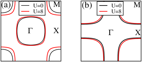
Figure S1: (a) FSs of $\psi_{S}$ at $U=0$ (black lines) and $U=8$ eV (red lines). (b) FSs of $\beta$ band at $U=0$ (black lines) and $U=8$ eV (red lines).

References

- Bednorz and Müller (1986) J. G. Bednorz and K. A. Müller, “Possible high tc superconductivity in the ba-la-cu-o system,” Zeitschrift für Physik B Condensed Matter 64, 189–193 (1986).
- Lee et al. (2006) Patrick A. Lee, Naoto Nagaosa, and Xiao-Gang Wen, “Doping a mott insulator: Physics of high-temperature superconductivity,” Rev. Mod. Phys. 78, 17–85 (2006).
- Keimer et al. (2015) B. Keimer, S. A. Kivelson, M. R. Norman, S. Uchida, and J. Zaanen, “From quantum matter to high-temperature superconductivity in copper oxides,” Nature 518, 179–186 (2015).
- Maeno et al. (1994) Y. Maeno, H. Hashimoto, K. Yoshida, S. Nishizaki, T. Fujita, J. G. Bednorz, and F. Lichtenberg, “Superconductivity in a layered perovskite without copper,” Nature 372, 532–534 (1994).
- Kamihara et al. (2008) Yoichi Kamihara, Takumi Watanabe, Masahiro Hirano, and Hideo Hosono, “Iron-based layered superconductor la[01-xfx]feas(x=0.05-0.12) with tc =26k,” Journal of the American Chemical Society 130, 3296–3297 (2008).
- Takahashi et al. (2008) Hiroki Takahashi, Kazumi Igawa, Kazunobu Arii, Yoichi Kamihara, Masahiro Hirano, and Hideo Hosono, “Superconductivity at 43 k in an iron-based layered compound lao1-xfxfeas,” Nature 453, 376–378 (2008).
- Paglione and Greene (2010) Johnpierre Paglione and Richard L. Greene, “High-temperature superconductivity in iron-based materials,” Nature Physics 6, 645–658 (2010).
- Hu et al. (2015) Jiangping Hu, Congcong Le, and Xianxin Wu, “Predicting unconventional high-temperature superconductors in trigonal bipyramidal coordinations,” Phys. Rev. X 5, 041012 (2015).
- Anisimov et al. (1999) V. I. Anisimov, D. Bukhvalov, and T. M. Rice, “Electronic structure of possible nickelate analogs to the cuprates,” Phys. Rev. B 59, 7901–7906 (1999).
- Lee and Pickett (2004) K.-W. Lee and W. E. Pickett, “Infinite-layer : is not ,” Phys. Rev. B 70, 165109 (2004).
- Crespin et al. (1983a) Michel Crespin, Pierre Levitz, and Lucien Gatineau, “Reduced forms of lanio3 perovskite. part 1.—evidence for new phases: La2ni2o5 and lanio2,” J. Chem. Soc., Faraday Trans. 2 79, 1181–1194 (1983a).
- Greenblatt (1997) Martha Greenblatt, “Ruddlesden-popper lnn+1nino3n+1 nickelates: structure and properties,” Current Opinion in Solid State and Materials Science 2, 174–183 (1997).
- Hayward et al. (1999) M. A. Hayward, M. A. Green, M. J. Rosseinsky, and J. Sloan, “Sodium hydride as a powerful reducing agent for topotactic oxide deintercalation: Synthesis and characterization of the nickel(i) oxide lanio2,” Journal of the American Chemical Society 121, 8843–8854 (1999).
- Crespin et al. (1983b) Michel Crespin, Pierre Levitz, and Lucien Gatineau, “Reduced forms of lanio3 perovskite. part 1.—evidence for new phases: La2ni2o5 and lanio2,” J. Chem. Soc., Faraday Trans. 2 79, 1181–1194 (1983b).
- Crespin et al. (2005) M. Crespin, O. Isnard, F. Dubois, J. Choisnet, and P. Odier, “Lanio2: Synthesis and structural characterization,” Journal of Solid State Chemistry 178, 1326–1334 (2005).
- Kawai et al. (2010) Masanori Kawai, Kazuya Matsumoto, Noriya Ichikawa, Masaichiro Mizumaki, Osami Sakata, Naomi Kawamura, Shigeru Kimura, and Yuichi Shimakawa, “Orientation change of an infinite-layer structure lanio2 epitaxial thin film by annealing with cah2,” Crystal Growth & Design 10, 2044–2046 (2010).
- Li et al. (2019) Danfeng Li, Kyuho Lee, Bai Yang Wang, Motoki Osada, Samuel Crossley, Hye Ryoung Lee, Yi Cui, Yasuyuki Hikita, and Harold Y. Hwang, “Superconductivity in an infinite-layer nickelate,” Nature 572, 624–627 (2019).
- Osada et al. (2020) Motoki Osada, Bai Yang Wang, Kyuho Lee, Danfeng Li, and Harold Y. Hwang, “Phase diagram of infinite layer praseodymium nickelate thin films,” Phys. Rev. Mater. 4, 121801 (2020).
- Li et al. (2020) Danfeng Li, Bai Yang Wang, Kyuho Lee, Shannon P. Harvey, Motoki Osada, Berit H. Goodge, Lena F. Kourkoutis, and Harold Y. Hwang, “Superconducting dome in infinite layer films,” Phys. Rev. Lett. 125, 027001 (2020).
- Norman (2020) Michael R. Norman, “Entering the Nickel Age of Superconductivity,” Physics 13, 85 (2020).
- Sun et al. (2023) Hualei Sun, Mengwu Huo, Xunwu Hu, Jingyuan Li, Zengjia Liu, Yifeng Han, Lingyun Tang, Zhongquan Mao, Pengtao Yang, Bosen Wang, Jinguang Cheng, Dao-Xin Yao, Guang-Ming Zhang, and Meng Wang, “Signatures of superconductivity near 80 k in a nickelate under high pressure,” Nature (2023), 10.1038/s41586-023-06408-7.
- Hou et al. (2023) J. Hou, P. T. Yang, Z. Y. Liu, J. Y. Li, P. F. Shan, L. Ma, G. Wang, N. N. Wang, H. Z. Guo, J. P. Sun, Y. Uwatoko, M. Wang, G. M. Zhang, B. S. Wang, and J. G. Cheng, “Emergence of high-temperature superconducting phase in the pressurized La3Ni2O7 crystals,” arXiv e-prints , arXiv:2307.09865 (2023), arXiv:2307.09865 [cond-mat.supr-con] .
- Zhang et al. (2023a) Yanan Zhang, Dajun Su, Yanen Huang, Hualei Sun, Mengwu Huo, Zhaoyang Shan, Kaixin Ye, Zihan Yang, Rui Li, Michael Smidman, Meng Wang, Lin Jiao, and Huiqiu Yuan, “High-temperature superconductivity with zero-resistance and strange metal behavior in La3Ni2O7,” arXiv e-prints , arXiv:2307.14819 (2023a), arXiv:2307.14819 [cond-mat.supr-con] .
- Luo et al. (2023) Zhihui Luo, Xunwu Hu, Meng Wang, Wéi Wú, and Dao-Xin Yao, “Bilayer two-orbital model of La3Ni2O7 under pressure,” arXiv e-prints , arXiv:2305.15564 (2023), arXiv:2305.15564 [cond-mat.supr-con] .
- Zhang et al. (2023b) Yang Zhang, Ling-Fang Lin, Adriana Moreo, and Elbio Dagotto, “Electronic structure, orbital-selective behavior, and magnetic tendencies in the bilayer nickelate superconductor La3Ni2O7 under pressure,” arXiv e-prints , arXiv:2306.03231 (2023b), arXiv:2306.03231 [cond-mat.supr-con] .
- Yang et al. (2023a) Qing-Geng Yang, Da Wang, and Qiang-Hua Wang, “Possible -wave superconductivity in La3Ni2O7,” arXiv e-prints , arXiv:2306.03706 (2023a), arXiv:2306.03706 [cond-mat.supr-con] .
- Sakakibara et al. (2023) Hirofumi Sakakibara, Naoya Kitamine, Masayuki Ochi, and Kazuhiko Kuroki, “Possible high superconductivity in La3Ni2O7 under high pressure through manifestation of a nearly-half-filled bilayer Hubbard model,” arXiv e-prints , arXiv:2306.06039 (2023), arXiv:2306.06039 [cond-mat.supr-con] .
- Gu et al. (2023) Yuhao Gu, Congcong Le, Zhesen Yang, Xianxin Wu, and Jiangping Hu, “Effective model and pairing tendency in bilayer Ni-based superconductor La3Ni2O7,” arXiv e-prints , arXiv:2306.07275 (2023), arXiv:2306.07275 [cond-mat.supr-con] .
- Shen et al. (2023) Yang Shen, Mingpu Qin, and Guang-Ming Zhang, “Effective bi-layer model Hamiltonian and density-matrix renormalization group study for the high-Tc superconductivity in La3Ni2O7 under high pressure,” arXiv e-prints , arXiv:2306.07837 (2023), arXiv:2306.07837 [cond-mat.str-el] .
- Christiansson et al. (2023) Viktor Christiansson, Francesco Petocchi, and Philipp Werner, “Correlated electronic structure of La3Ni2O7 under pressure,” arXiv e-prints , arXiv:2306.07931 (2023), arXiv:2306.07931 [cond-mat.str-el] .
- Shilenko and Leonov (2023) D. A. Shilenko and I. V. Leonov, “Correlated electronic structure, orbital-selective behavior, and magnetic correlations in double-layer La3Ni2O7 under pressure,” arXiv e-prints , arXiv:2306.14841 (2023), arXiv:2306.14841 [cond-mat.str-el] .
- Wú et al. (2023) Wéi Wú, Zhihui Luo, Dao-Xin Yao, and Meng Wang, “Charge Transfer and Zhang-Rice Singlet Bands in the Nickelate Superconductor under Pressure,” arXiv e-prints , arXiv:2307.05662 (2023), arXiv:2307.05662 [cond-mat.str-el] .
- Cao and Yang (2023) Yingying Cao and Yi-feng Yang, “Flat bands promoted by Hund’s rule coupling in the candidate double-layer high-temperature superconductor La3Ni2O7,” arXiv e-prints , arXiv:2307.06806 (2023), arXiv:2307.06806 [cond-mat.supr-con] .
- Chen et al. (2023) Xuejiao Chen, Peiheng Jiang, Jie Li, Zhicheng Zhong, and Yi Lu, “Critical charge and spin instabilities in superconducting La3Ni2O7,” arXiv e-prints , arXiv:2307.07154 (2023), arXiv:2307.07154 [cond-mat.supr-con] .
- Liu et al. (2023) Yu-Bo Liu, Jia-Wei Mei, Fei Ye, Wei-Qiang Chen, and Fan Yang, “The s±-Wave Pairing and the Destructive Role of Apical-Oxygen Deficiencies in La3Ni2O7 Under Pressure,” arXiv e-prints , arXiv:2307.10144 (2023), arXiv:2307.10144 [cond-mat.supr-con] .
- Lu et al. (2023) Chen Lu, Zhiming Pan, Fan Yang, and Congjun Wu, “Interlayer Coupling Driven High-Temperature Superconductivity in La3Ni2O7 Under Pressure,” arXiv e-prints , arXiv:2307.14965 (2023), arXiv:2307.14965 [cond-mat.supr-con] .
- Zhang et al. (2023c) Yang Zhang, Ling-Fang Lin, Adriana Moreo, Thomas A. Maier, and Elbio Dagotto, “Structural phase transition, -wave pairing and magnetic stripe order in the bilayered nickelate superconductor La3Ni2O7 under pressure,” arXiv e-prints , arXiv:2307.15276 (2023c), arXiv:2307.15276 [cond-mat.supr-con] .
- Oh and Zhang (2023) Hanbit Oh and Ya-Hui Zhang, “Type II t-J model and shared antiferromagnetic spin coupling from Hund’s rule in superconducting La3Ni2O7,” arXiv e-prints , arXiv:2307.15706 (2023), arXiv:2307.15706 [cond-mat.str-el] .
- Liao et al. (2023) Zhiguang Liao, Lei Chen, Guijing Duan, Yiming Wang, Changle Liu, Rong Yu, and Qimiao Si, “Electron correlations and superconductivity in La3Ni2O7 under pressure tuning,” arXiv e-prints , arXiv:2307.16697 (2023), arXiv:2307.16697 [cond-mat.supr-con] .
- Qu et al. (2023) Xing-Zhou Qu, Dai-Wei Qu, Jialin Chen, Congjun Wu, Fan Yang, Wei Li, and Gang Su, “Bilayer -- Model and Magnetically Mediated Pairing in the Pressurized Nickelate La3Ni2O7,” arXiv e-prints , arXiv:2307.16873 (2023), arXiv:2307.16873 [cond-mat.str-el] .
- Yang et al. (2023b) Yi-feng Yang, Guang-Ming Zhang, and Fu-Chun Zhang, “Minimal effective model and possible high- mechanism for superconductivity of La3Ni2O7 under high pressure,” arXiv e-prints , arXiv:2308.01176 (2023b), arXiv:2308.01176 [cond-mat.supr-con] .
- Fujimori and Minami (1984) Atsushi Fujimori and Fujio Minami, “Valence-band photoemission and optical absorption in nickel compounds,” Phys. Rev. B 30, 957–971 (1984).
- van Elp et al. (1992) J. van Elp, H. Eskes, P. Kuiper, and G. A. Sawatzky, “Electronic structure of li-doped nio,” Phys. Rev. B 45, 1612–1622 (1992).
- Kuiper et al. (1989) P. Kuiper, G. Kruizinga, J. Ghijsen, G. A. Sawatzky, and H. Verweij, “Character of holes in and their magnetic behavior,” Phys. Rev. Lett. 62, 221–224 (1989).
- Taguchi et al. (2008) M. Taguchi, M. Matsunami, Y. Ishida, R. Eguchi, A. Chainani, Y. Takata, M. Yabashi, K. Tamasaku, Y. Nishino, T. Ishikawa, Y. Senba, H. Ohashi, and S. Shin, “Revisiting the valence-band and core-level photoemission spectra of nio,” Phys. Rev. Lett. 100, 206401 (2008).
- Zhang and Rice (1988) F. C. Zhang and T. M. Rice, “Effective hamiltonian for the superconducting cu oxides,” Phys. Rev. B 37, 3759–3761 (1988).
- Anderson et al. (2004) P W Anderson, P A Lee, M Randeria, T M Rice, N Trivedi, and F C Zhang, “The physics behind high-temperature superconducting cuprates: the ‘plain vanilla’ version of rvb,” Journal of Physics: Condensed Matter 16, R755 (2004).
- Jiang et al. (2018) Kun Jiang, Xianxin Wu, Jiangping Hu, and Ziqiang Wang, “Nodeless high- superconductivity in the highly overdoped monolayer,” Phys. Rev. Lett. 121, 227002 (2018).
- Jiang et al. (2021) Kun Jiang, Congcong Le, Yinxiang Li, Shengshan Qin, Ziqiang Wang, Fuchun Zhang, and Jiangping Hu, “Electronic structure and two-band superconductivity in unconventional high- cuprates ,” Phys. Rev. B 103, 045108 (2021).