Fréchet Statistics Based Change Point Detection in Multivariate Hawkes Process

Abstract

This paper proposes a new approach for change point detection in causal networks of multivariate Hawkes processes using Fréchet statistics. Our method splits the point process into overlapping windows, estimates kernel matrices in each window, and reconstructs the signed Laplacians by treating the kernel matrices as the adjacency matrices of the causal network. We demonstrate the effectiveness of our method through experiments on both simulated and real-world cryptocurrency datasets. Our results show that our method is capable of accurately detecting and characterizing changes in the causal structure of multivariate Hawkes processes, and may have potential applications in fields such as finance and neuroscience. The proposed method is an extension of previous work on Fréchet statistics in point process settings and represents an important contribution to the field of change point detection in multivariate point processes.

1 Introduction

Complex systems often exhibit a series of events that unfold over time, causing a ripple effect throughout the system. These chains of events are a prominent characteristic of various real-world networks, including social, biological, and financial networks. For instance, within social networks, a reciprocal action may set off a chain of retaliatory responses, potentially escalating into serious gang conflicts [1], the formation of polarized echo chambers [2, 3], or the propagation of misinformation [4]. Similarly, neuron activity in the brain can trigger a cascade of stimulations or inhibitions in other neurons, resulting in a wide range of outcomes [5]. Moreover, the stock market is also an example of a system where an initial shock can lead to a contagion of volatility throughout the financial network [6].

To better understand and model the occurrence of such events, multivariate Hawkes processes have become increasingly popular. They are a class of stochastic point processes that capture self- and mutual-excitatory behaviors and are used to model complex interactions between multiple channels in various fields such as neuroscience, finance, and social science. The multivariate Hawkes process provides a flexible framework to capture the cascading or clustering effects that arise when the occurrence of an event in one channel triggers events in other channels.

Change point detection for multivariate Hawkes process is a critical problem in various fields such as finance, social science, and neuroscience. Existing methods rely on estimating the kernel functions of the process using generalized likelihood ratio (GLR) or CUSUM procedure. However, in this study, we propose a new approach that reconstructs the integral of the kernel function by matching cumulants and uses it to infer changes in location and scale by analyzing the corresponding signed Laplacian matrices’ Fréchet statistics. This approach relaxes the need for fully recovering the kernel function and offers a novel way of identifying changes in multivariate time series.

The key idea of the proposed change point approach is to treat the reconstructed kernel integral matrix as the causal network or latent structure of the process. By using the Fréchet statistics of the corresponding signed Laplacian matrices, we can infer changes in both location and scale. This approach provides a more flexible way of detecting change points in multivariate Hawkes processes and can provide insights into the underlying causal relationships between the different dimensions of the process. By applying this method to real-world datasets, we demonstrate its effectiveness and its ability to identify important changes in the data.

Main Results and Organization:

(1) In Section 2, we define a multivariate Hawkes process and kernel functions. We define the kernel matrix as the integral of the kernel functions, which represents the underlying causal structure among various dimensions of the process. We then use the NPHC algorithm [7] to estimate the kernel matrix based on cumulants matching of the process in Section 2.1, which removes the need to fully recover the kernel functions.

(2) In Section 3, we treat the estimated kernel matrix as the adjacency matrix of the causal network, and propose a metric space for the corresponding signed Laplacian. Log-Euclidean metric is used to measure their distances. This allows us to derive a closed-form formula for Fréchet mean and variance under this metric, which provides a more accurate and efficient way of measuring the distances between causal networks.

(3) Finally, in Section 4, we validate our proposed method on simulated datasets as well as real-world cryptocurrency datasets, including the price of 41 DeFi coins spanning a period of 13 months. We confirm the method’s performance through ground truth change points in simulation and real events for the real-world datasets.

Related Works:

Change point detection in point processes has been a topic of considerable interest in the literature. The aim is to identify points in time when the statistical properties of the point process change abruptly. Change points can provide important insights into the underlying process and help in predicting future behavior. In recent years, there has been an increasing interest in the detection of change points in multivariate point processes, particularly in Hawkes processes.

One popular approach to change point detection in point processes is based on the likelihood ratio test (LRT). The LRT is a non-parametric method that can be used to detect changes in the intensity function of the point process. It has been successfully applied to a wide range of point processes, including Poisson processes and Hawkes processes. For example, a recent study by Yamin et al. [8] proposed a methodology to detect supply chain network disruptions caused by the COVID-19 pandemic. The authors use a modified CUSUM and a LRT-based method on the order data of a furniture company modeled using the Hawkes Process Network. Wang et al. [9] proposed a CUSUM procedure for sequential change-point detection in Hawkes networks using discrete events data. The authors propose a method that can detect changes in the intensity function of the point process based on the LRT.

Another popular approach to change point detection in point processes is based on the Bayesian framework. Bayesian methods offer several advantages, including the ability to incorporate prior information and the ability to handle complex models. Li et al. [10] proposed a non-parametric Bayesian approach to detect change-points of intensity rates in the recurrent-event context and cluster subjects by the change points. The proposed model provides an objective way of clustering subjects based on the change-points without the need for pre-specifying the number of latent clusters or model selection procedure. A recent study by Detommaso [11] proposed a Stein variational online changepoint detection (SVOCD) method, which extends Bayesian online changepoint detection (BOCPD) beyond the exponential family of probability distributions. The method integrates Stein variational Newton (SVN) and BOCPD to offer a full online Bayesian treatment in various applications, including Hawkes processes and long short-term memory (LSTM) neural networks. Linderman et al. [12] used random graph model as a prior to enable the analysis of latent networks of multivariate Hawkes processes. The method enables sparse network but cannot model the directed connections.

In addition to the LRT and Bayesian approaches, there are other methods for change point detection in point processes, including spectral methods, clustering methods, and non-parametric methods. For example, Cribben and Yu [13] introduced a data-driven method called Network Change Points Detection (NCPD), which detects change points in the network structure of a multivariate time series. They used a spectral clustering approach for unveiling the community structure in the network and reducing the data dimension. NCPD is applied to various simulated data and a resting-state fMRI data set.

Overall, change point detection in point processes, particularly in Hawkes processes, is an active area of research, with many promising methods being developed. These methods have the potential to provide important insights into the underlying processes and aid in predicting future behavior.

2 Multivariate Hawkes Process

In this section, we outline the formulation of a multivariate Hawkes process. Let $(\Omega,{\mathcal{F}},P)$ be a complete probability space and consider a multivariate Hawkes process $N(t)=(N_{1},\cdots,N_{m})$, where $N_{i}(t),1\leq i\leq m$, is the counting process representing the cumulative number of events up to time $t$ for subject $i$. We define a set of increasing $\sigma$-algebras $\{{\mathcal{F}}^{t}\}_{t\geq 0}$, where ${\mathcal{F}}^{t}=\sigma\{N^{t}\}$, and the non-negative, ${\mathcal{F}}^{t}$-measurable process $\lambda(t)$ as the intensity of $N(t)$, given by:

$$\begin{split}P(dN_{i}(t)=1|{\mathcal{F}}^{t})&=\lambda_{i}(t)dt+o(dt),\\ P(dN_{i}(t)>1|{\mathcal{F}}^{t})&=o(dt),\end{split}$$ (1)

where $o(dt)$ is little-o of $dt$ and $\lim\limits_{dt\rightarrow 0}\frac{o(dt)}{dt}=0$. The intensity $\lambda_{i}(t)$ for each subject is given by:

$$\lambda_{i}(t)=\mu_{i}+\sum_{j=1}^{m}\int_{0}^{t}\phi_{ij}(t-s)dN_{j}(s),$$ (2)

where $\mu_{i}$ is the background rate and $\phi_{ij}(\cdot)$ is the kernel function representing the effects of process $N_{j}$ on process $N_{i}$. We interpret the integral in (2) as a Stieltjes integral [14].

A popular choice for $\phi_{ij}(\cdot)$ is an exponential function $\phi_{ij}(t)=\alpha_{ij}e^{-\beta_{ij}t}$, and (2) can be rewritten as

$$\lambda_{i}(t)=\mu_{i}+\sum_{j=1}^{m}\int_{0}^{t}\alpha_{ij}e^{-\beta_{ij}(t-s)}dN_{j}(s).$$ (3)

We can represent (2) in matrix form as:

$$\lambda(t)=\mu+\int_{0}^{t}\boldsymbol{\phi}(t-s)dN(s),$$ (4)

where $\boldsymbol{\phi}(\cdot)$ is an $m\times m$ kernel matrix with entries $\phi_{ij}(\cdot)$.

This matrix representation (4) provides a concise way of expressing the intensity of a multivariate Hawkes process. Furthermore, recent work [15] has shown that $\boldsymbol{\phi}(\cdot)$ (which they referred to as the excitation matrix) with exponential kernel functions (3) can reveal the casual structure underlying the multivariate components. Specifically, $N_{i}(t)$ is Granger non-causal for $N_{j}(t)$ if and only if the corresponding kernel function $\phi_{ij}(\cdot)=0$ (See Definition 2. Granger causality for Hawkes processes in [7]).

To infer the causal structure from $\boldsymbol{\phi}(\cdot)$, we use the integrals of its elements to construct the matrix $H=[h_{ij}]$, where

$$h_{ij}=\int_{0}^{\infty}\phi_{ij}(t)dt.$$ (5)

For kernels with exponential functions (3), we have $h_{ij}=\frac{\alpha_{ij}}{\beta_{ij}}$. $h_{ij}$ is commonly referred to as the branching ratio, which quantifies the average number of events triggered by a single event, providing a measure of the endogenous effect in finance [16]. Furthermore, the cluster representation of Hawkes processes [17] reveals that the integral in the expression for the intensity of a multivariate Hawkes process signifies the average total number of events for subject $i$ that are directly triggered by an event for subject $j$.

2.1 Kernel Matrix Estimation based on Integrated Cumulants

The Non-Parametric Hawkes with Cumulants (NPHC) algorithm, introduced in [7], is a moment-matching method that facilitates the estimation of the kernel matrix $H$ without the need to estimate the kernel functions’ shape. The primary idea behind this method is that the integrated cumulants of a Hawkes process can be expressed explicitly as a function of $H$, as shown in [18].

For an arbitrary $m$-dimensional random vector $X=(X_{1},\cdots,X_{m})$, the cumulant of order $m$, denoted by $k(X_{\bar{m}})$, where $\bar{m}$ indicates the set $\{1,\cdots,m\}$, is defined as

$$k(X_{\bar{m}})=\sum_{\pi}(|\pi|-1)!(-1)^{|\pi|-1}\prod_{B\in\pi}\langle X_{B}\rangle,$$ (6)

where the sum goes over all partitions $\pi$ of the set $\{1,\cdots,m\}$, $|\cdot|$ denotes the number of blocks of a given partition, and $\langle X_{B}\rangle=\langle\prod_{k\in B}X_{k}\rangle$. The integrated cumulants provide a measure of the average correlated activity between events of different subjects, which is a natural generalization of the covariance of two variables to higher dimensions.

Note that if $H$ has a spectral radius $\rho$ strictly smaller than 1, $N(t)$ has asymptotically stationary increments, and $\lambda(t)$ is asymptotically stationary [19]. Consequently, $R=(I_{d}-H)^{-1}$ can be defined.

The first three integrated cumulants of a multivariate Hawkes process can be used to estimate the mean intensity, integrated covariance density matrix, and skewness of the process. T by equations (7), (8), and (9), respectively. Due to the process’s stationarity, these relationships are given by [7]:

$$\Lambda_{i}dt =\mathop{\mathbb{E}}\left[dN_{i}(t)\right],$$ (7)

$$C_{ij}dt =\int\limits_{\tau\in\mathbb{R}}\mathop{\mathbb{E}}\left[dN_{i}(t)dN_{j}(t+\tau)\right]-\mathop{\mathbb{E}}\left[dN_{i}(t)\right]\mathop{\mathbb{E}}\left[dN_{j}(t+\tau)\right],$$ (8)

$$K_{ijk}dt =\int\limits_{\tau\in\mathbb{R}}\int\limits_{\tau^{\prime}\in\mathbb{R}}\mathop{\mathbb{E}}\left[dN_{i}(t)dN_{j}(t+\tau)dN_{k}(t+\tau^{\prime})\right]$$

$$\phantom{----}+2\mathop{\mathbb{E}}\left[dN_{i}(t)\right]\mathop{\mathbb{E}}\left[dN_{j}(t+\tau)\right]\mathop{\mathbb{E}}\left[dN_{k}(t+\tau^{\prime})\right]$$

$$\phantom{----}-\mathop{\mathbb{E}}\left[dN_{i}(t)dN_{j}(t+\tau)\right]\mathop{\mathbb{E}}\left[dN_{k}(t+\tau^{\prime})\right]$$

$$\phantom{----}-\mathop{\mathbb{E}}\left[dN_{i}(t)dN_{k}(t+\tau^{\prime})\right]\mathop{\mathbb{E}}\left[dN_{j}(t+\tau)\right]$$

$$\phantom{----}-\mathop{\mathbb{E}}\left[dN_{j}(t+\tau)dN_{k}(t+\tau^{\prime})\right]\mathop{\mathbb{E}}\left[dN_{i}(t)\right],$$ (9)

Specifically, the mean intensity $\Lambda_{i}$ and the integrated covariance density matrix $C_{ij}$ can be expressed as linear combinations of the vector of background intensities $\mu$ and the matrix $R_{ij}$, while the skewness $K_{ijk}$ can be expressed as a polynomial in $R_{ij}$ and $C_{ij}$ [7]:

$$\Lambda_{i} =\sum_{l=1}^{m}R_{il}\mu_{l},$$ (10)

$$C_{ij} =\sum_{l=1}^{m}\Lambda_{l}R_{il}R_{jl},$$ (11)

$$K_{ijk} =\sum_{1=1}^{m}(R_{il}R_{jl}C_{kl}+R_{il}C_{jl}R_{kl}+C_{il}R_{jl}R_{kl}$$

$$\phantom{-------------}-2\Lambda_{l}R_{il}R_{jl}R_{kl}).$$ (12)

The estimation procedure assumes that truncating the integration from $(-\infty,+\infty)$ to $[-W,W]$ in (8) and (9) introduces only a small error. Given a realization of a stationary Hawkes process $N(t),t\in[0,T]$, where $Z_{i}$ represents the set of events corresponding to subject $i$, the estimators for the three cumulants (7), (8), and (9) can be obtained under this assumption:

$$\hat{\Lambda}_{i} =\frac{N_{i}(T)}{T},$$ (13)

$$\hat{C}_{ij} =\frac{1}{T}\sum_{\tau\in Z_{i}}(N_{j}(\tau+W)-N_{j}(\tau-W)-2W\hat{\Lambda}_{j}),$$ (14)

$$\hat{K}_{ijk} =\frac{1}{T}\sum_{\tau\in Z_{i}}\Big{[}(N_{j}(\tau+W)-N_{j}(\tau-W)-2W\hat{\Lambda}_{j})$$

$$\phantom{----}.(N_{k}(\tau+W)-N_{k}(\tau-W)-2W\hat{\Lambda}_{k})\Big{]}$$

$$\phantom{--}-\frac{\hat{\Lambda}_{i}}{T}\sum_{\tau\in Z_{j}}\sum_{\tau^{\prime}\in Z_{k}}(2W-|\tau^{\prime}-\tau|)^{+}+4W^{2}\hat{\Lambda}_{i}\hat{\Lambda}_{j}\hat{\Lambda}_{k}.$$ (15)

Since the covariance $C$ provides fewer independent coefficients than the kernel matrix $H$, the NPHC algorithm focuses on a subset of $m^{2}$ third-order cumulant coefficients $K_{iij}$, namely $K^{c}=\{K_{iij}\}_{1\leq i,j\leq m}$. Specifically, the estimator of $R$, denoted $\hat{R}$, is obtained by minimizing the Frobenius norm of two differences:

$$\begin{split}\hat{R}&=\operatorname*{arg\,min}_{R}\mathcal{L}(R)\\ &=\operatorname*{arg\,min}_{R}(1-\kappa)\|K^{c}(R)-\hat{K^{c}}\|_{2}^{2}+\kappa\|C(R)-\hat{C}\|_{2}^{2},\end{split}$$ (16)

where $\|\cdot\|_{2}$ represents the Frobenius norm, while $\hat{C}$ and $\hat{K^{c}}$ are the respective estimators of $C$ and $K^{c}$ as defined in (14), (15).

Finally, once $\hat{R}$ is obtained, the kernel matrix $H$ can be estimated as $\hat{H}=I_{m}-\hat{R}^{-1}$, where $I_{d}$ is the identity matrix of size $m\times m$.

Remark: In [16, 20], the filtering parameter $W$ is chosen based on estimates of the covariance density at multiple time points $t$. Specifically, they compute the estimate $\hat{C}_{ij}(t)$ as follows:

$$\hat{C}_{ij}(t)=\frac{1}{\delta T}\sum_{\tau\in Z_{i}}(N_{j}(\tau+t+\delta)-N_{j}(\tau+t)-\delta\hat{\Lambda}_{j}),$$ (17)

where $\delta$ is a small constant. The characteristic time $\tau_{c}$ is used to determine the time interval $W$ over which the covariance density is considered significant. A multiple of $\tau_{c}$ is typically selected as $W$, such as $W=5\tau_{c}$. Empirical studies have shown that $W$ can be chosen to be several orders of magnitude larger than the average inter-event time [20].

3 Fréchet Statistics Based Change Point Detection

In this section, we propose a change point detection method that utilizes the Fréchet statistics of a sequence of causal networks. We construct these networks using the estimated kernel matrix $\hat{H}$ obtained in Section 2.1. By computing the Fréchet distance between the signed Laplacian matrices of these networks, we can detect significant changes in the underlying structure of the multivariate Hawkes process.

3.1 Dynamic Causal Network

A dynamic causal network is a sequence of graph snapshots $G^{(1)},G^{(2)},\cdots$, where each snapshot $G^{(t)}=(V^{(t)},E^{(t)})$ represents the causal network observed at time $t$. To ensure that all graph snapshots have the same set of vertices, we require that $V^{(1)}=V^{(2)}=\cdots=V$, meaning that the multivariate Hawkes process arises from a fixed set of subjects.

To construct a snapshot of the causal network, we use a sliding window approach. Specifically, we estimate the kernel matrix $\hat{H}$ from a sliding window of the multivariate Hawkes process and take the symmetric part, $A=(\hat{H}+\hat{H}^{T})/2$, as the adjacency matrix for the snapshot of the causal network. Each element $a_{ij}$ in $A$ represents the weight of the edge from node $i$ to node $j$. $a_{ij}>0$ denotes a positive edge, and $a_{ij}<0$ denotes a negative edge.

Denote $A^{(t)}$ as the adjacency matrix of the causal network during the $t$-th sliding window. The signed Laplacian $\bar{L}^{(t)}$ is defined as $\bar{L}^{(t)}=\bar{D}^{(t)}-A^{(t)}$, where $\bar{D}^{(t)}$ is the diagonal degree matrix given by $\bar{d}^{(t)}{ii}=\sum{j=1}^{m}|a^{(t)}_{ij}|$, that is, the diagonal entries are the unsigned degree of each node.

3.2 Fréchet Mean of Signed Laplacian Matrices

To measure the dissimilarity between two snapshots in a dynamic causal network, we define a metric space [21] based on the Log-Euclidean metric of the nearest symmetric positive definite (SPD) matrices of their corresponding signed Laplacian matrices. The introduced metric enables us to compare the structures of different snapshots of the dynamic causal network. Moreover, it admits a closed-form Fréchet mean, which enables efficient computation.

The signed Laplacian matrix $\bar{L}^{(t)}$ is known to be positive semi-definite [22], which can cause problems when using SPD metrics like the Log-Euclidean metric. To address this issue, we adopt the algorithm proposed by Cheng and Higham [23] to find the nearest symmetric positive definite (SPD) matrix to $\bar{L}^{(t)}$ in the Frobenius norm. The resulting SPD matrix, denoted by $\tilde{L}^{(t)}$, is used instead of $\bar{L}^{(t)}$ to define the metric space.

We introduce a metric space $({\tilde{\mathcal{L}}},{\textrm{d}})$ for dynamic causal networks. Here, ${\tilde{\mathcal{L}}}$ denotes the set of nearest symmetric positive definite (SPD) matrices to the signed Laplacians, and d is a function ${\textrm{d}},\colon{\tilde{\mathcal{L}}}\times{\tilde{\mathcal{L}}}\to\mathbb{R}{+}$ defined using the Log-Euclidean metric, i.e., $\delta{LE}(X,Y)=|\log(X)-\log(Y)|_{\textrm{F}}$.

Suppose we have a set of independent and identically distributed random variables ${\tilde{L}}^{(1)},\cdots,{\tilde{L}}^{(n)}\sim F$ in $({\tilde{\mathcal{L}}},{\textrm{d}})$. According to Theorem 3.13 in [24], the metric space $({\tilde{\mathcal{L}}},{\textrm{d}})$ admits a unique closed-form Fréchet mean $\mu_{F}$, which is given by $\mu_{F}=\exp(\mathbb{E}(\log({\tilde{L}})))$. We also define the sample Fréchet mean as $\hat{\mu}F=\exp(\frac{1}{n}\sum{i=1}^{n}\log({\tilde{L}}^{(i)}))$. The existence and uniqueness of the sample Fréchet mean imply its asymptotic consistency [25].

The Fréchet variance quantifies the spread of a random variable around its Fréchet mean. For ${\tilde{L}}^{(1)},\cdots,{\tilde{L}}^{(n)}\sim F$, we define the population Fréchet variance as $V_{F}=\mathbb{E}({\textrm{d}}^{2}(\mu_{F},{\tilde{L}}))$ and the sample Fréchet variance as $\hat{V}F=\frac{1}{n}\sum{i=1}^{n}{\textrm{d}}^{2}(\hat{\mu}F,{\tilde{L}}^{(i)})=\frac{1}{n}\sum{i=1}^{n}|\frac{1}{n}\sum_{j=1}^{n}\log({\tilde{L}}^{(j)})-\log({\tilde{L}}^{(i)})|_{\textrm{F}}^{2}$.

Under certain assumptions (Assumptions 1-3 in [26]), we establish the Central Limit Theorem for the sample Fréchet variance $\hat{V}_{F}$ in the metric space $({\tilde{\mathcal{L}}},{\textrm{d}})$. Specifically, we have $n^{1/2}(\hat{V}_{F}-V_{F})\rightarrow N(0,\sigma^{2}_{F})$ in distribution, where $\sigma^{2}_{F}=\textrm{Var}{{\textrm{d}}^{2}(\mu_{F},{\tilde{L}})}$. For a detailed proof, please refer to [26].

3.3 Estimating the Location of a Change Point

Let us consider a sequence $\{Y^{(i)}\}_{i=1}^{n}$ of independent, time-ordered data points in a metric space $({\tilde{\mathcal{L}}},{\textrm{d}})$ defined in Section 3.2. We assume there is at most one change point, which we denote by $0<\tau<1$. Specifically, $Y^{(1)},\cdots,Y^{(\lfloor n\tau\rfloor)}\sim F_{1}$ and $Y^{(\lfloor n\tau\rfloor+1)},\cdots,Y^{(n)}\sim F_{2}$, where $F_{1}$ and $F_{2}$ are unknown probability measures on $({\tilde{\mathcal{L}}},{\textrm{d}})$, and $\lfloor x\rfloor$ is the greatest integer less than or equal to $x$. Our aim is to test the null hypothesis of distribution homogeneity, denoted by $H_{0}:F_{1}=F_{2}$, against the alternative hypothesis of a single change point, denoted by $H_{1}:F_{1}\neq F_{2}$.

We constrain the hypothesized change point location $\tau$ to a compact interval $\mathcal{I}_{c}=[c,1-c]\subset[0,1]$ with positive constant $c$ to ensure accurate representation of each segment’s Fréchet mean and variance. For statistical analysis of segments separated by $u\in\mathcal{I}_{c}$, we compute the sample Fréchet mean before and after $\lfloor nu\rfloor$ observations as:

$$\begin{split}\hat{\mu}_{[0,u]}&=\operatorname*{arg\,min}\limits_{l\in{\tilde{\mathcal{L}}}}\frac{1}{\lfloor n\tau\rfloor}\sum\limits_{i=1}^{\lfloor n\tau\rfloor}{\textrm{d}}^{2}(Y^{(i)},l),\\ \hat{\mu}_{[u,1]}&=\operatorname*{arg\,min}\limits_{l\in{\tilde{\mathcal{L}}}}\frac{1}{n-\lfloor n\tau\rfloor}\sum\limits_{i=\lfloor n\tau\rfloor+1}^{n}{\textrm{d}}^{2}(Y^{(i)},l),\end{split}$$

and the corresponding sample Fréchet variances are:

$$\begin{split}\hat{V}_{[0,u]}&=\frac{1}{\lfloor n\tau\rfloor}\sum\limits_{i=1}^{\lfloor n\tau\rfloor}{\textrm{d}}^{2}(Y^{(i)},\hat{\mu}{[0,u]}),\\ \hat{V}_{[u,1]}&=\frac{1}{n-\lfloor n\tau\rfloor}\sum\limits_{i=\lfloor n\tau\rfloor+1}^{n}{\textrm{d}}^{2}(Y^{(i)},\hat{\mu}_{[u,1]}),\end{split}$$ (18)

One can obtain the contaminated version of Fréchet variances by replacing the Fréchet mean of a segment with the mean of the complementary segment. This leads to the definitions:

$$\begin{split}\hat{V}^{C}_{[0,u]}&=\frac{1}{\lfloor n\tau\rfloor}\sum\limits_{i=1}^{\lfloor n\tau\rfloor}{\textrm{d}}^{2}(Y^{(i)},\hat{\mu}{[u,1]}),\\ \hat{V}^{C}_{[u,1]}&=\frac{1}{n-\lfloor n\tau\rfloor}\sum\limits_{i=\lfloor n\tau\rfloor+1}^{n}{\textrm{d}}^{2}(Y^{(i)},\hat{\mu}{[0,u]}),\end{split}$$

which are guaranteed to be at least as large as the correct version (18). The differences $\hat{V}^{C}_{1}-\hat{V}_{[0,u]}$ and $\hat{V}^{C}_{2}-\hat{V}_{[u,1]}$ can be interpreted as measures of the between-group variance of the two segments.

For some fixed $u\in\mathcal{I}_{c}$, the statistic $\sqrt{u(1-u)}(\sqrt{n}/\sigma)(\hat{V}_{[0,u]}-\hat{V}_{[u,1]})$ has an asymptotic standard normal distribution under the null hypothesis $H_{0}$. Here, $\sigma$ denotes the asymptotic variance of the empirical Fréchet variance. This result allows us to test hypotheses about differences in Fréchet variances between two segments of data. A sample based estimator for $\sigma^{2}$ is:

$$\hat{\sigma}^{2}=\frac{1}{n}\sum_{i=1}^{n}{\textrm{d}}^{4}(\hat{\mu},{\tilde{L}}_{i})-\left(\frac{1}{n}\sum_{i=1}^{n}{\textrm{d}}^{2}(\hat{\mu},{\tilde{L}}_{i})\right)^{2},$$

which is consistent under $H_{0}$ [26]. Also,

$$\hat{\mu}=\operatorname*{arg\,min}\limits_{l\in{\tilde{\mathcal{L}}}}\frac{1}{n}\sum\limits_{i=1}^{n}{\textrm{d}}^{2}(Y^{(i)},l),\quad\hat{V}=\frac{1}{n}\sum\limits_{i=1}^{n}{\textrm{d}}^{2}(Y^{(i)},\hat{\mu}).$$

The test statistic proposed in [27] can detect differences in both Fréchet means and Fréchet variances of the distributions $F_{1}$ and $F_{2}$. The equation for the test statistic is provided as follows:

$$\begin{split}T_{n}(u)=&\frac{u(1-u)}{\hat{\sigma}^{2}}\Big{[}(\hat{V}_{[0,u]}-\hat{V}_{[u,1]})^{2}\\ &\phantom{---}+(\hat{V}_{[0,u]}^{C}-\hat{V}_{[0,u]}+\hat{V}_{[u,1]}^{C}-\hat{V}_{[u,1]})^{2}\Big{]}\end{split}$$ (19)

In this equation, $(\hat{V}_{[0,u]}-\hat{V}_{[u,1]})^{2}$ indicates the difference in Fréchet variances between two segments of data, while $(\hat{V}_{[0,u]}^{C}-\hat{V}_{[0,u]}+\hat{V}_{[u,1]}^{C}-\hat{V}_{[u,1]})^{2}$ captures the difference in Fréchet means between the two segments.

Theorem 1 in [27] demonstrates that under $H_{0}$, ${nT_{n}(u):u\in\mathcal{I}_{c}}$ weakly converges to the square of a standardized Brownian bridge on the interval $\mathcal{I}_{c}$, which is given by:

$$\mathcal{G}=\left\{\frac{\mathcal{B}(u)}{\sqrt{u(1-u)}}:u\in\mathcal{I}_{c}\right\},$$

where ${\mathcal{B}(u):u\in\mathcal{I}_{c}}$ is a Brownian bridge on $\mathcal{I}_{c}$, which is a Gaussian process indexed by $\mathcal{I}_{c}$ with zero mean and covariance structure given by $K(s,t)=\min(s,t)-st$.

To perform a hypothesis test between $H_{0}$ and $H_{1}$, the statistic $\sup_{u\in\mathcal{I}_{c}}nT_{n}(u)$ is used. Here, $T_{n}(u)$ is a test statistic for the hypothesis test, which is computed for each potential change point $u\in\mathcal{I}_{c}$. The $(1-\alpha)$th quantile of $\sup_{u\in\mathcal{I}_{c}}\mathcal{G}^{2}(u)$ is denoted as $q_{1-\alpha}$, which is obtained by a bootstrap approach, as described in Section 3.3 of [27].

Under the null hypothesis $H_{0}$, the following weak convergence holds:

$$\sup_{u\in\mathcal{I}_{c}}nT_{n}(u)\Rightarrow\sup_{u\in\mathcal{I}_{c}}\mathcal{G}^{2}(u),$$ (20)

where $T_{n}(u)$ is the test statistic and $\mathcal{G}^{2}(u)$ is the limiting distribution. We use this result to define the rejection region for a level $\alpha$ significance test as:

$$R_{n,\alpha}=\left\{\sup_{u\in\mathcal{I}_{c}}nT_{n}(u)>q_{1-\alpha}\right\},$$ (21)

where $q_{1-\alpha}$ is the $(1-\alpha)$ quantile of $\mathcal{G}^{2}(u)$.

Under the alternative hypothesis $H_{1}$, which assumes a change point is present at $\tau\in\mathcal{I}_{c}$, we can locate it by finding the maximizer of the process $T_{n}(u)$:

$$\hat{\tau}=\operatorname*{arg\,max}_{u\in\mathcal{I}_{c}}T_{n}(u)=\operatorname*{arg\,max}_{\lfloor nc\rfloor\leq k\leq n-\lfloor nc\rfloor}T_{n}\left(\frac{k}{n}\right),$$ (22)

where $\hat{\tau}$ is the estimated change point that maximizes the test statistic across all potential change points.

We refer the interested reader to [21] (Algorithm 1) for a binary segmentation procedure that extends the proposed statistic $T_{n}(u)$ (19) to the multiple change point scenario.

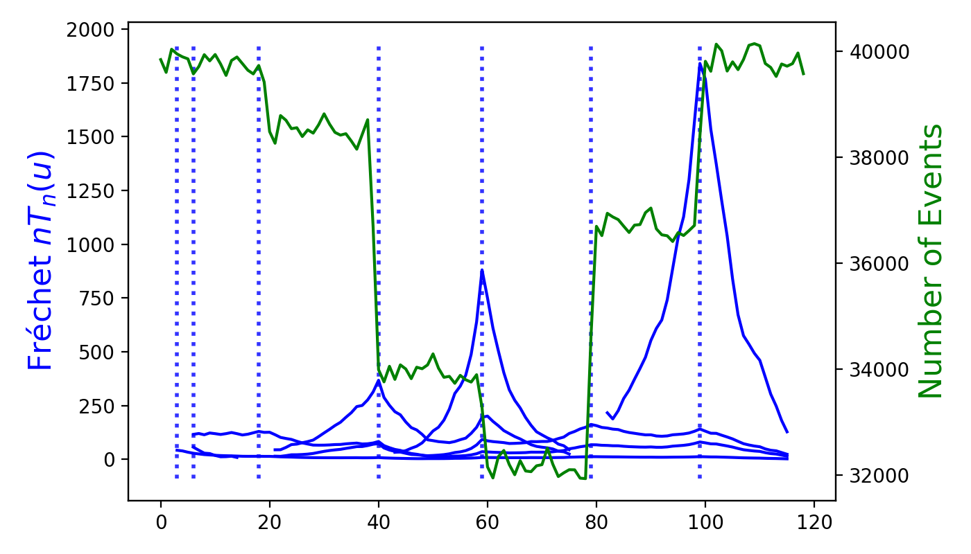
Figure 1: Our algorithm effectively detected all change points in a synthetic 10-dimensional point process of length 600000 using Fréchet statistics. The data was split into 119 overlapping windows of length 10000, with the number of events in each window shown in green. The accuracy of our algorithm was verified by the ground truth. The Fréchet test statistic ${nT_{n}(u):u\in\mathcal{I}_{c}}$ was also plotted for each analyzed segment due to the use of binary segmentation.

4 Empirical Analysis on Simulated and Real-world Networks

We evaluate the performance of the proposed method on change point detection on both a simulated dataset and a real-world cryptocurrency market dataset. Our results are completely reproducible; the code and datasets used in the experiments are publicly available at https://tinyurl.com/Hawkes-Change.

4.1 Simulation Study

We generated a synthetic dataset using the multivariate Hawkes process model, implemented through the Python library tick. We first set the base intensities $\lambda_{i}$ for all 10 subjects to be 0.3. We then defined the kernel function using an exponential decay model, as shown in (3), with decay parameters $\beta_{ij}=0.5+u_{ij}$, where $u_{ij}$ is sampled from a uniform distribution between 0 and 1.

To set the amplitude of the kernel function, we used the following values: for $i=j$, $\hat{\alpha}_{ij}=1/8$, and for $i\neq j$, $\hat{\alpha}_{ij}$ was sampled from a normal distribution with mean 0 and variance $1/64$. We symmetrized these values to obtain $\alpha_{ij}=(\hat{\alpha}_{ij}+\hat{\alpha}_{ji})/2$. We ensured that the spectral radius of the resulting kernel matrix $H$ was less than 1, which guarantees the stationarity of the process. The integral of each kernel function is computed as $h_{ij}=\frac{\alpha_{ij}}{\beta_{ij}}$.

We induce change points by updating the $\alpha_{ij}$ every 100000 units, resulting in a modification of the causal network $H$ of the process.

To evaluate the performance of our algorithm in detecting multiple change points, we analyze a simulated multivariate process of length 600000. The data is divided into overlapping windows of length 10000, with adjacent windows having an overlapping window of length 5000. Figure 1 shows that the Fréchet statistics based algorithms accurately detect all the change points, as confirmed by the ground truth generated during dataset construction. We also plot the test statistics, that is, the Fréchet test statistic ${nT_{n}(u):u\in\mathcal{I}_{c}}$ (19) for our algorithm. Since we use binary segmentation, we display the Fréchet test statistic for each analyzed segment.

4.2 Cryptocurrency Price Data

We use Binance’s cryptocurrency price data for 41 DeFi-related coins. The data was sampled every 5 minutes for 396 days between March 2022 and March 2023. Events were identified whenever a coin price changed by $\pm 0.5\%$ of its current price, resulting in a 41-dimensional multivariate point process. We divided the process into 56 overlapping 2-week windows with 1-week overlap for adjacent windows.

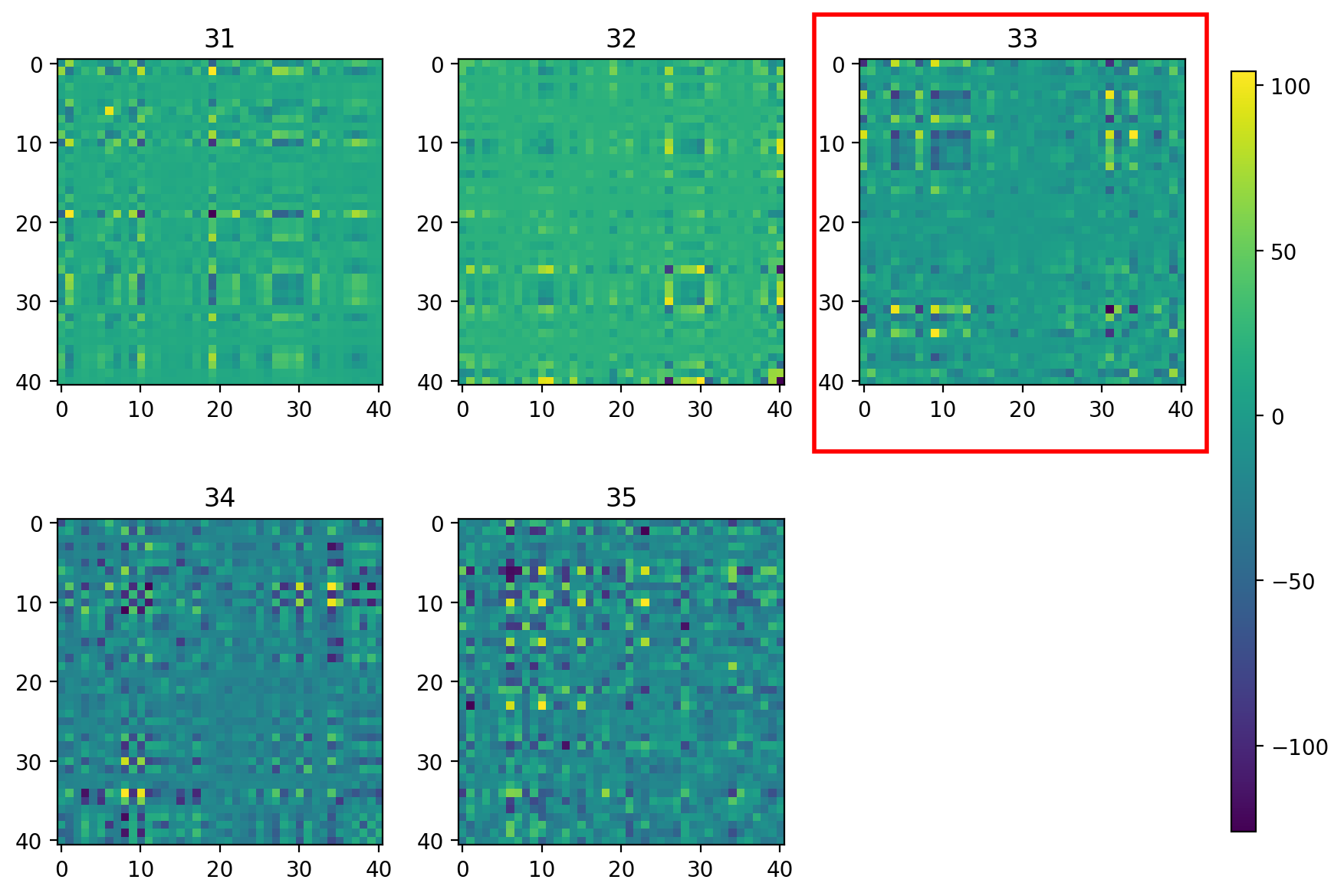
Figure 2: The sequence of symmetrized kernel matrices $A^{(t)}=(H^{(t)}+{H^{(t)}}^{T})/2$ estimated by the NPHC algorithm (see Section 2.1) is displayed before and after the detected change point at time 33. The change in the underlying causal network dynamics is reflected in the shift of the kernel matrix patterns from the earlier (left) to the later (right) time periods.

We present the results of our analysis of the cryptocurrency price dataset using a 41-dimensional multivariate Hawkes process model. Figure 3 displays the multiple change points detected in the model, which highlight periods of increased activity and volatility in the cryptocurrency market. To better understand the underlying dynamics, we show the adjacency matrices of the causal network of the multivariate Hawkes process before and after one of the detected change points in Figure 2.

To validate the detected change points, we cross-referenced them with significant events in the cryptocurrency market, as summarized in Table 1. Our findings offer valuable insights into the communication patterns and organizational behavior during market transformations or even crashes, and demonstrate the potential of multivariate Hawkes process models in capturing the complex dynamics of financial markets.

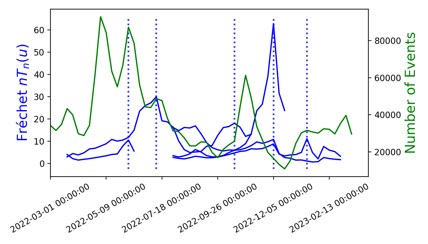
Figure 3: Result of our algorithm for detecting multiple change points of the cryptocurrency price dataset. The number of events in each window is displayed in green.

Start Date	No.	Event
06/06/2022	14	Terra-LUNA contagion.
07/11/2022	19	Voyager and Celsius filed for bankruptcy.
10/17/2022	33	Over US$718 million stolen from decentralized finance.
12/05/2022	40	BlockFi, which had taken a US$250 million loan from FTX, declared bankruptcy.
01/16/2023	46	Bitcoin price is up 39% since the start of January.

TABLE I: Timeline of events related to the cryptocurrency market, which serves as the ground truth change points for the analysis presented in Fig. 3.

5 Conclusions

In this study, we propose a method for detecting change points in causal networks of multivariate Hawkes processes using Fréchet statistics. Specifically, we divide the point process into a sequence of overlapping windows, estimate the kernel matrices in each window, and reconstruct the signed Laplacians by treating the kernel matrices as the graph adjacency matrices of the causal network. Our method builds upon the previous work of Luo et al. [21] and Dubey et al. [27], and extends it to multivariate point process settings.

To validate the effectiveness of our method, we evaluate it on both simulated and real-world datasets. The simulated dataset is used to assess the method’s ability to accurately detect change points under controlled conditions, while the real-world cryptocurrency dataset provides a challenging testbed for analyzing complex, high-dimensional data. Our results demonstrate that the proposed method is a powerful tool for detecting and characterizing changes in the causal structure of multivariate Hawkes processes, with potential applications in finance, neuroscience, and other fields.

References

- [1] J. Randle and G. Bichler, “Uncovering the social pecking order in gang violence,” Crime prevention in the 21st century: Insightful approaches for crime prevention initiatives, pp. 165–186, 2017.
- [2] R. Luo, B. Nettasinghe, and V. Krishnamurthy, “Echo chambers and segregation in social networks: Markov bridge models and estimation,” IEEE Transactions on Computational Social Systems, 2021.
- [3] ——, “Controlling segregation in social network dynamics as an edge formation game,” IEEE transactions on network science and engineering, vol. 9, no. 4, pp. 2317–2329, 2022.
- [4] R. Luo and V. Krishnamurthy, “Mitigating misinformation spread on blockchain enabled social media networks,” arXiv preprint arXiv:2201.07076, 2022.
- [5] S. W. Linderman, “Bayesian methods for discovering structure in neural spike trains,” Ph.D. dissertation, Harvard University, 2016.
- [6] R. Luo, V. Krishnamurthy, and E. Blasch, “Hawkes process modeling of block arrivals in bitcoin blockchain,” arXiv preprint arXiv:2203.16666, 2022.
- [7] M. Achab, E. Bacry, S. Gaıffas, I. Mastromatteo, and J.-F. Muzy, “Uncovering causality from multivariate hawkes integrated cumulants,” in International Conference on Machine Learning. PMLR, 2017, pp. 1–10.
- [8] K. Yamin, H. Wang, B. Montreuil, and Y. Xie, “Online detection of supply chain network disruptions using sequential change-point detection for hawkes processes,” arXiv preprint arXiv:2211.12091, 2022.
- [9] H. Wang, L. Xie, Y. Xie, A. Cuozzo, and S. Mak, “Sequential change-point detection for mutually exciting point processes,” Technometrics, pp. 1–13, 2022.
- [10] Q. Li, F. Guo, and I. Kim, “A non-parametric bayesian change-point method for recurrent events,” Journal of Statistical Computation and Simulation, vol. 90, no. 16, pp. 2929–2948, 2020.
- [11] G. Detommaso, H. Hoitzing, T. Cui, and A. Alamir, “Stein variational online changepoint detection with applications to hawkes processes and neural networks,” arXiv preprint arXiv:1901.07987, 2019.
- [12] S. Linderman and R. Adams, “Discovering latent network structure in point process data,” in International conference on machine learning. PMLR, 2014, pp. 1413–1421.
- [13] I. Cribben and Y. Yu, “Estimating whole-brain dynamics by using spectral clustering,” Journal of the Royal Statistical Society. Series C (Applied Statistics), pp. 607–627, 2017.
- [14] M. Dresher, The mathematics of games of strategy. Courier Corporation, 2012.
- [15] J. Etesami, N. Kiyavash, K. Zhang, and K. Singhal, “Learning network of multivariate hawkes processes: A time series approach,” arXiv preprint arXiv:1603.04319, 2016.
- [16] S. J. Hardiman and J.-P. Bouchaud, “Branching-ratio approximation for the self-exciting hawkes process,” Physical Review E, vol. 90, no. 6, p. 062807, 2014.
- [17] A. G. Hawkes and D. Oakes, “A cluster process representation of a self-exciting process,” Journal of applied probability, vol. 11, no. 3, pp. 493–503, 1974.
- [18] S. Jovanović, J. Hertz, and S. Rotter, “Cumulants of hawkes point processes,” Physical Review E, vol. 91, no. 4, p. 042802, 2015.
- [19] A. G. Hawkes, “Spectra of some self-exciting and mutually exciting point processes,” Biometrika, vol. 58, no. 1, pp. 83–90, 1971.
- [20] M. Achab, E. Bacry, J.-F. Muzy, and M. Rambaldi, “Analysis of order book flows using a non-parametric estimation of the branching ratio matrix,” Quantitative Finance, vol. 18, no. 2, pp. 199–212, 2018.
- [21] R. Luo and V. Krishnamurthy, “Fréchet statistics based change point detection in dynamic social networks,” 2023.
- [22] J. Kunegis, S. Schmidt, A. Lommatzsch, J. Lerner, E. W. De Luca, and S. Albayrak, “Spectral analysis of signed graphs for clustering, prediction and visualization,” in Proceedings of the 2010 SIAM international conference on data mining. SIAM, 2010, pp. 559–570.
- [23] S. H. Cheng and N. J. Higham, “A modified cholesky algorithm based on a symmetric indefinite factorization,” SIAM Journal on Matrix Analysis and Applications, vol. 19, no. 4, pp. 1097–1110, 1998.
- [24] V. Arsigny, P. Fillard, X. Pennec, and N. Ayache, “Geometric means in a novel vector space structure on symmetric positive-definite matrices,” SIAM journal on matrix analysis and applications, vol. 29, no. 1, pp. 328–347, 2007.
- [25] A. Petersen and H.-G. Müller, “Fréchet regression for random objects with Euclidean predictors,” The Annals of Statistics, vol. 47, no. 2, pp. 691 – 719, 2019. [Online]. Available: https://doi.org/10.1214/17-AOS1624
- [26] P. Dubey and H.-G. Müller, “Fréchet analysis of variance for random objects,” Biometrika, vol. 106, no. 4, pp. 803–821, 2019.
- [27] ——, “Fréchet change-point detection,” The Annals of Statistics, vol. 48, no. 6, pp. 3312 – 3335, 2020. [Online]. Available: https://doi.org/10.1214/19-AOS1930
- [28] P. Billingsley, Convergence of probability measures. John Wiley & Sons, 2013.