An Adaptive Phase-Field Method for Structural Topology Optimization††thanks: The work of B. Jin is supported by a start-up fund and Direct Grant for Research 2022/2023, both from The Chinese University of Hong Kong. The work of Y. Xu was supported in part by the National Natural Science Foundation of China (12250013, 12261160361 and 12271367) and the Science and Technology Commission of Shanghai Municipality (17ZR1420800, 20JC1413800 and 22ZR1445400). The work of S. Zhu was supported in part by the National Key Basic Research Program (2022YFA1004402), the National Natural Science Foundation of China (12071149) and the Science and Technology Commission of Shanghai Municipality (21JC1402500, 22ZR1421900 and 22DZ2229014).
Abstract
In this work, we develop an adaptive algorithm for the efficient numerical solution of the minimum compliance problem in topology optimization. The algorithm employs the phase field
approximation and continuous density field. The adaptive procedure is driven by two
residual type a posteriori error estimators, one for the state variable and the other for the
objective functional. The adaptive algorithm is provably convergent in the sense that the
sequence of numerical approximations generated by the adaptive algorithm contains a
subsequence convergent to a solution of the continuous first-order optimality system. We provide
several numerical simulations to show the distinct features of the algorithm.
Keywords: minimum compliance, adaptive algorithm, topology optimization, convergence, a posteriori error estimator
1 Introduction
This work is concerned with effective numerical algorithms for the classical minimum compliance problem in structural topology optimization, which is a highly active research area in engineering. It mainly deals with the optimal distribution of materials over a given design domain. Over the last few decades, this area has witnessed significant advances, and found a broad range of practical applications, e.g., in mechanics, heat transfer, acoustics and electromagnetics; see, e.g., the reviews [22, 39] and the monograph [6, 37] on various theoretical and practical issues of the discipline.
The minimum compliance problem, first introduced by the pioneering work [4], is one fundamental formulation in topology optimization. The goal is to find the optimal distribution of isotropic material that minimizes the work of the external forces at equilibrium, with a prescribed amount of volume. Often an optimization problem is formulated by penalizing elastic properties of the medium that depends on the local values of the density field. There are several popular material interpolation schemes, including SIMP (Solid Isotropic Material with Penalization) [3, 51, 5] and RAMP (Rational Approximation of Material Properties) [43], etc.
Among the different ways to formulate the minimum compliance problem, we focus on the phase-field approximation, which employs a smooth function, i.e., material density function, to describe the distribution of two phases, representing the material and void inside the design domain, and encodes the geometrical information associated with the optimal topology in the sharp interfaces between the two phases. Methodologically, it penalizes the objective functional by a functional approximating the total variation of the material density function, which, in the sharp-interface limit, measures the perimeter of the interfaces between the material and void [7]. The relaxed functional consists of two terms controlling the width of the interfaces and the decomposition of the pure phases. Distinct features of the approach include that it greatly facilitates relevant theoretical analysis, e.g., well-posedness of the formulation and the convergence analysis of discrete approximation, and it eventually provides optimal solutions at the discrete level free from mesh dependency and checkerboard phenomena. The use of the phase-field approach in topology optimization was first introduced for design dependent loads [8, 9], problems with stress constraints [13] and minimum compliance case [50, 52]; see the works [45, 20, 48, 49, 46, 38, 32, 25] for several contributions.
Numerically, one popular strategy for topology optimization is discretize-and-then-optimize: first discretizes the density field and state variable and then optimize the resulting finite-dimensional optimization problem. The discretization often employs finite element methods (FEMs) to approximate the state variable and the density, and the same mesh is generally used for both. For the minimum compliance problem, the standard approach implements low-order displacement-based finite elements and element-wise density discretization (i.e., piecewise constant). The degree of freedom of the resulting discretization(s) directly determines the computational cost of the overall procedure. Finer meshes improve the accuracy of the geometric description and the approximation of mechanical behavior, but involve a larger number of density and displacement unknowns and thus increase the overall computational complexity for the optimizer and finite element solver. The approximation of the state variable is nontrivial due to the nearly piecewise constant nature of the elastic properties and geometrical variations, which tend to induce weak singularities in the solution along the interfaces. Thus, it is highly nontrivial to specify meshes a priori for computational efficiency.
One promising idea to tackle the computational challenge is adaptivity, which has been explored in several recent works [17, 42, 18, 12, 30, 19]. Costa and Alves [17] described an adaptive algorithm combining topology optimization and a Zienkiewicz-Zhu based -refinement technique, which however, does not include coarsening void regions and filtering procedures, which hence exhibits undesirable mesh-dependence convergence behaviour. Stainko [42] proposed an adaptive multilevel refinement driven by the detection of the evolving solid-void interface based on RAMP-based filtering scheme and linear material interpolation. de Sturler et al. [18] showed the advantage provided by coarsening operations within the cavities of the optimal design and commented on the need for uniform refinement in and around the full material zones, in order to avoid convergence to sub-optimal results that may arise in early coarse grids. Bruggi and Verani [12] presented a fully adaptive topology optimization algorithm using goal-oriented error control in order to simultaneously ensure accurate geometrical description and compliance approximation. Lambe and Czekanski [30] studied adaptive mesh refinement using different analysis and design meshes, based on Helmholtz type density filter. de Troya and Tortorelli [19] presented a structural optimization framework with adaptive mesh refinement and stress constraints. All these proposals have demonstrated impressive empirical performance under various problem settings in that the obtained optimal designs are comparable with that by uniform meshes but at a much reduced computational expense. However, the rigorous convergence analysis is unavailable for all these algorithms. This is largely due to the incorporation of ad hoc filtering procedures in the algorithms for overcoming numerical instabilities (e.g., checkboard), and also since the error estimators are derived in a heuristic manner, especially for geometric description [42, 12]. Hence, there is still a demand in developing provably convergent adaptive topology optimization algorithms.
Motivated by these observations, we propose in this work a novel adaptive algorithm for the volume-constrained minimum compliance problem using the phase field approximation, and call the resulting algorithm an adaptive phase-field method. The proposed algorithm consists of an iterative procedure of the following form
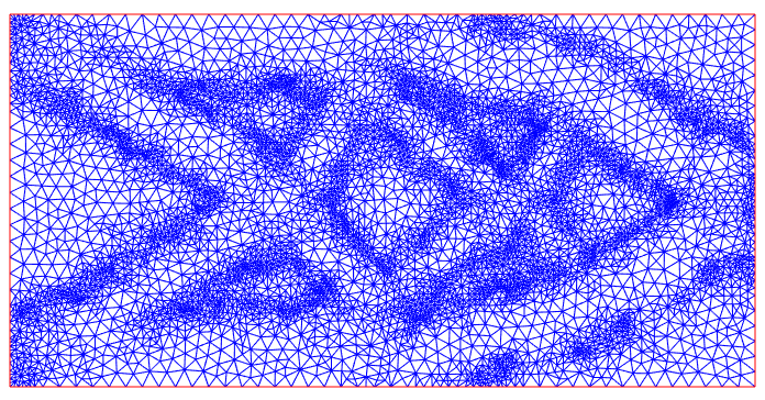
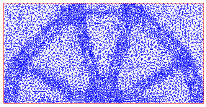
The algorithm employs the same triangulation of simplicial elements for approximating the density and displacement field. The four modules in the loop are defined as follows. The module OPTIMIZE solves a well-posed minimization problem based on the phase-field approximation on the underlying mesh using techniques from mathematical programming. (In contrast, in several existing adaptive techniques, this step employs ad hoc filtering techniques to tackle numerical instabilities.) The module ESTIMATE computes two error estimators of residual type [1, 47], one for the error due to the finite element approximation of the displacement field, and the other for the variational inequalities in the first-order necessary optimality system. These two estimators drive the whole adaptive procedure and are derived via a careful analysis of the necessary optimality system. Thus, the proposed algorithm provides an adaptive discretization that iteratively improves the geometrical description and the approximation of mechanical behavior. The module REFINE refines the marked elements within the triangulation (by the module MARK) to produce a locally refined mesh. Typical meshes show concentrated refinement layer near the boundaries of the optimal design with a variable size mesh within the bulk, depending on the strain energy density.
Numerical simulations on six benchmark problems show that the proposed adaptive algorithm can find the layout of the optimal design in the first few iterations, and improve the accuracy of the final results at later iterations. The obtained optimal designs present topological and compliance errors that are quantitatively comparable with that based on uniform meshes of larger scale, but at a reduced computational cost. Further, compared with existing adaptive techniques [17, 42, 18, 12, 30, 19], we derive the error estimators rigorously, and prove the convergence of the proposed adaptive algorithm in the following sense: the sequence of discrete approximations generated by the algorithm contains a subsequence convergent to a solution of the necessary optimality system; See Section 5 for the detailed proof. This result is viable only for the phase field approximation, and not for the filter-based approach, for which there seems no known convergence result, even for the case of uniform mesh. The adaptive algorithm and its convergence analysis represent the main contributions of this work. To the best of our knowledge, this work presents a first provably convergent adaptive algorithm for a topology optimization problem.
The rest of the paper is organized as follows. In Section 2, we describe fundamentals of the volume-constrained minimum compliance problem, recalling both continuous and discrete formulations. Then in Section 3, we present the proposed adaptive algorithm, and derive suitable error estimators. In Section 4, we present extensive numerical simulations to demonstrate the excellent performances of the adaptive algorithm, and compare it with relevant uniform refinement. In Section 5, we present the technical and lengthy convergence analysis of the algorithm.
2 Mathematical formulation
2.1 Minimum compliance problem
Let be an open bounded domain. The boundary consists of two disjoint open sets and and . Loaded with a body force and a traction and clamped on the boundary , the elastic structure occupying the domain is described by the linear elasticity theory in the stress-displacement formulation:
| (2.1) |
where denotes the displacement field at equilibrium, the related strain field is given by
is the stress field and is the unit outward normal on the boundary , and the superscript denotes the matrix transpose. Different from the standard linear elasticity theory, in topology optimization, the elastic tensor depends on the density field. There are several different parameterizations, and we adopt the popular SIMP model [3], which takes the following form
where is the density field taking two values in almost everywhere in with , is a penalization parameter that is usually assumed to be equal to 3 [6], and is a symmetric fourth-order elastic tensor of an isotropic medium, given by
with being Lamé constants, being the trace operator of a second-order tensor field and being the identity matrix. The weak formulation of problem (2.1) reads: find such that
| (2.2) |
The unique solvability of (2.2) is guaranteed by Korn’s inequality (e.g., [10, 11, 15, 16]) and Lax-Milgram theorem. In topology optimization, it is common to impose constraint on the volume of the design domain, i.e., the total volume of the design material is fixed. Thus the admissible set for the density is given by
with being the total amount of material available for design.
The minimum compliance problem is to minimize the elastic potential energy
over the admissible set subject to the variational formulation (2.2). However, it is well-known that this problem is ill-posed in the sense that generally there is no minimizer within the admissible set [6]. Numerically, the corresponding numerical scheme often suffers from instabilities like checkerboard and mesh dependence, reminiscent of the ill-posedness of the continuous optimization problem. In practice, these drawbacks may be overcome via suitable filtering procedures (applied to the finite-dimensional discrete problem) [21, 41, 31] or penalization techniques (on the perimeters) [8, 9].
In this work, we follow the penalization strategy pioneered by [8, 9]. It is well known within the community of ill-posed problems that one powerful approach to remedy ill-posedness is regularization [27]. Below we regularize the objective functional with a total variation penalty, following the pioneering works [8, 9], which is consistent with the piecewise constant nature of the design (density field). This naturally leads to the following minimization problem:
| (2.3) |
where is the regularizing parameter, and is the total variation seminorm (or Radon measure of the distributional derivative), defined by
Then the space is defined by
with the associated norm defined by .
The next result gives the continuity of the parameter-to-state map . Then by a standard argument in calculus of variation, the compact embedding of the space into the space and the fact that -convergence implies almost everywhere convergence up to a subsequence [23], one can show the existence of a minimizer to the penalized problem (2.3). Thus, the penalized problem (2.3) is well-posed.
Lemma 2.1.
If the sequence converges to in and almost everywhere, then the sequence converges to in .
2.2 Phase field approximation
The numerical treatment of the total variation penalty is highly nontrivial, since the density is piecewise constant almost everywhere in the domain . In practice, it is often more convenient to relax the formulation via the phase field approximation. Specifically we further take a phase-field approximation to the functional , where the total variation seminorm in (2.3) is approximated by a Modica–Mortola type functional [35, 34]
with being a small number, controlling the width of the interface between the void and the material, and given by a double-well potential
The functional was first used by Cahn and Hilliard [14] to study the mixture of two immiscible fluids in the phase field theory. It is well-known that the sequence -converges to in with the constant [33]. The relaxed optimization problem is then given by
| (2.4a) | |||
| (2.4b) | |||
where solves the variaitonal formulation (2.2), and the relaxed admissible set is defined as
By repeating the argument for Lemma 2.1, we have the following continuity result with in place of .
Lemma 2.2.
If converges to in and almost everywhere, then the sequence converges to in .
Proof.
Since the functional is nonnegative, there exists a minimizing sequence such that . If , the statement holds trivially. Now we assume . This implies , which, along with the bound and the fact the domain is bounded, yields . Since is a closed convex set, there exists a subsequence, again labeled by , and some such that
Since , the sequence is uniformly bounded and converges to almost everywhere in . Then by Lebesgue’s dominated convergence theorem [23, Theorem 1.19], we have . By Lemma 2.2 and the weak lower semi-continuity of the norm, we further obtain
Upon recalling , this completes the proof of the theorem. ∎
2.3 Finite element approximation
Let be a shape regular conforming triangulation of the closure into closed triangles. Over the triangulation , we define a continuous piecewise linear finite element space
where is the set of linear polynomials on . The space is used for approximating the displacement field , whereas the discrete admissible set for approximating the density field is given by
Then the discrete approximation of problem (2.4a)–(2.4b) is given by
| (2.6a) | |||
| (2.6b) | |||
Like in the continuous case, the discrete problem (2.6a)–(2.6b) has at least one minimizer, since it is a finite-dimensional optimization problem and the objective is continuous and coercive. Further, for any given , it follows directly from Korn’s inequality and Lax-Milgram theorem that
| (2.7) |
The discrete optimization problem (2.6a)–(2.6b) can be solved by any standard optimization algorithms from mathematical programming, e.g., method of moving asymptotes [44] and CONLIN [24]. The computational complexity of these algorithms depends directly on the number of design parameters (for parameterizing the density field ), and implicitly on the degree of freedom of the finite element system. Since the optimal design is nearly piecewise constant, and has large jumps across the interfaces between void and material, the state variable will exhibit weak solution singularity in these regions, according to the classical elliptic regularity theory [26], which requires a fairly refined mesh for adequate resolution. This naturally motivates the use of a posteriori error estimator to drive an adaptive procedure.
3 Adaptive phase–field method
In this section, we propose a novel adaptive strategy for the finite element approximation (2.6a)–(2.6b).
3.1 Adaptive phase-field method
Let be a shape regular conforming triangulation of the domain into closed triangles such that the boundary is exactly covered by the restriction of on the boundary , and be the set of all possible conforming triangulations of obtained from by the successive use of bisection. Then the set is uniformly shape regular, i.e., the shape regularity of any mesh is bounded by a constant depending only on [36].
To describe the new adaptive algorithm for problem (2.4a)–(2.4b), we introduce some notations. The collection of all edges (respectively all interior edges) in is denoted by (respectively ) and its restriction to by , respectively. An edge has a fixed unit normal vector in with on . Over any triangulation , we define a piecewise constant mesh size function by
| (3.1) |
Since is shape regular, is equivalent to the diameter of any .
For the solution pair of problem (2.6a)–(2.6b), we define two element residuals for each element and two face residuals for each face by
where denotes the jumps across an interior faces . Then for any collection of elements , we define the following error estimator
| (3.2) |
with the estimators and given by
When , the notation will be suppressed. The estimator consists of two error indicators and . Roughly speaking, the former measures the error of approximating the objective functional , whereas the latter quantifies the discretizaion error of the state equation (2.2), similar to the standard residual estimators for elliptic PDEs [1, 47].
We next motivate the two a posteriori error estimators. Since is a minimizer pair of (2.6a)-(2.6b), it also satisfies the discrete optimality system
| (3.3) |
with given by . Using the variational inequality of (3.3), we may further deduce that for any ,
Here is an appropriate interpolant of (see (5.22) below). Moreover invoking the relevant error estimates in Lemma 5.4 and elementwise integration by parts (see the proof of Lemma 5.3), we can conclude
By the second equation of (3.3), a similar argument yields
Thus two computable quantities, i.e., and , are available to bound the two residuals associated with the optimality system (2.5). More importantly, the above derivation provides a crucial strategy to the convergence analysis in Section 5 even though and are not reliable (upper) bounds of -errors for the minimizer and the associated displacement field in any classical sense [1, 47].
Now we can present an adaptive algorithm for problem (2.4a)–(2.4b). All dependence on a triangulation is indicated by the iteration number in the subscript. In the module MARK, we adopt a separate marking by a comparison of the two estimators and . The marking is performed for the greater one by a bulk criterion or Dörfler’s strategy, and the adaptive algorithm is driven by the dominant term in the estimator.
| (3.4) |
| (3.5) |
We specify a maximum iteration number in the input of Algorithm 1 for termination. An alternative choice as the stopping criterion might be a prescribed tolerance for , or a given bound for the number of vertices of . We have the following theorem on the convergence of the numerical approximations . The proof is lengthy and technical and thus it is deferred to Section 5.
3.2 Implementation details of the module SOLVE
Now we present the details for solving the constrained minimization problem (2.4a)–(2.4b) based on a gradient flow type algorithm. To handle the volume constraint , we use the standard augmented Lagrangian method [28]. To this end, we define a Lagrangian by
| (3.7) |
where , is the associated Lagrange multiplier, and is a penalty parameter. The first-order optimality condition for an optimal phase-field function satisfies the following nonlinear system: for all
In the computation, we update the variables , , and alternatingly. We denote by , and the approximations at the th iteration, respectively. We first solve for the th linear elasticity , and then obtain and successively. Clearly, the crucial step is to minimize the Lagrangian with respect to the density . This step is performed by solving the following parabolic PDE, a gradient-descent flow:
| (3.8) |
where is the pseudo time and is the initial guess. To solve (3.8), we employ an inner iteration index such that the whole optimization algorithm has a nested inner-outer iteration framework. The semi-implicit variational formulation of problem (3.8) is to find such that for all :
| (3.9) |
with the initial data approximated by the standard projection of , where is a small time step. This semi-implicit scheme is typically evolved several (e.g., ) steps for fixed . Numerically we observe that the density function may do not preserve the box constraint . To remedy the issue, we perform a projection step:
Set after steps of (3.9). The Lagrange multiplier is updated using a Uzawa type scheme:
The value of increases (respectively decreases) as the current structure volume is larger (respectively smaller) than the target volume . The penalty parameter is updated during iterations:
Now we can state the whole algorithm on a fixed mesh in Algorithm 2. Then, Algorithm 1 for the adaptive phase field optimization model can be described specifically with the module SOLVE implemented by Algorithm 2.
4 Numerical results and discussions
In this section, we present several examples in topology optimization to demonstrate the performance of Algorithm 1. All numerical simulations are performed using MATLAB R2020a on a laptop with an Intel (R) Core (TM) i5-7500U CPU and 8 GB memory. The Lamé constants and in the elasticity tensor of the isotropic medium are taken to be
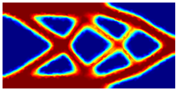
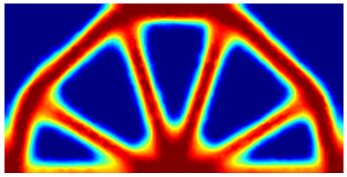
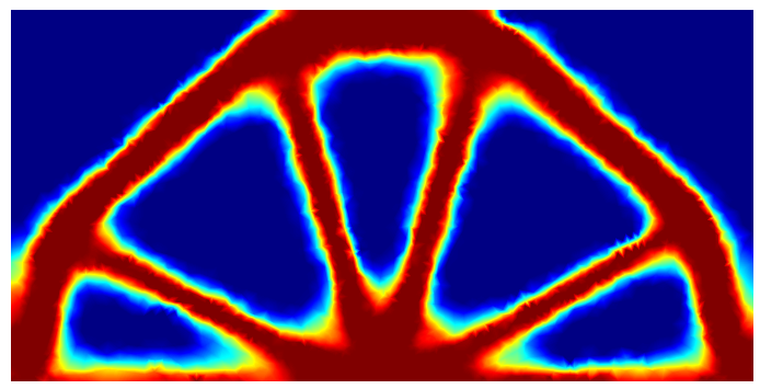
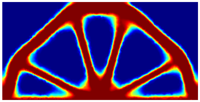
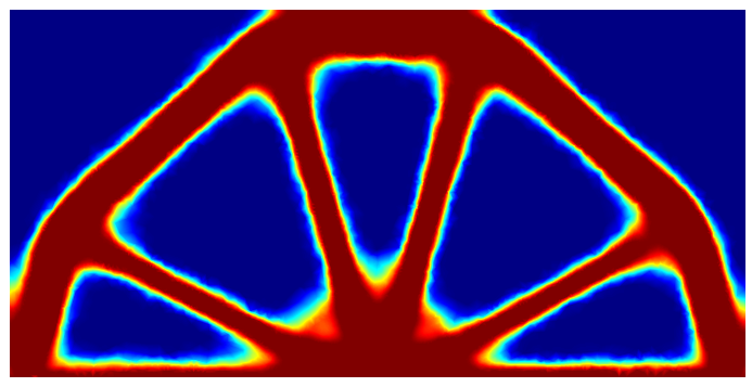
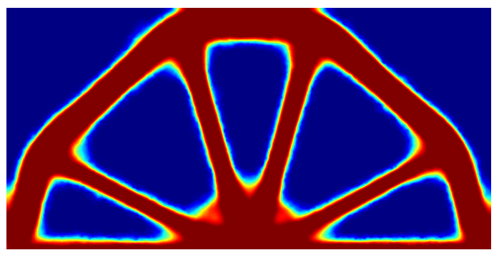
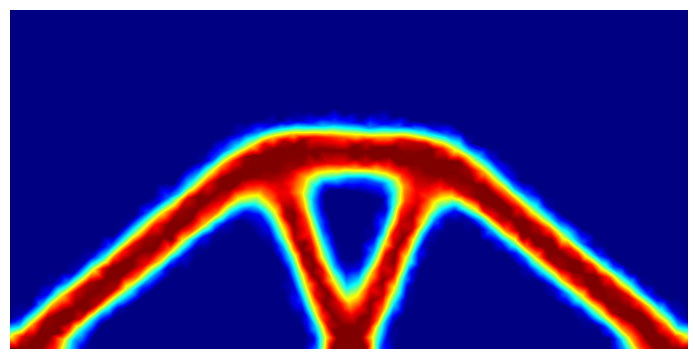
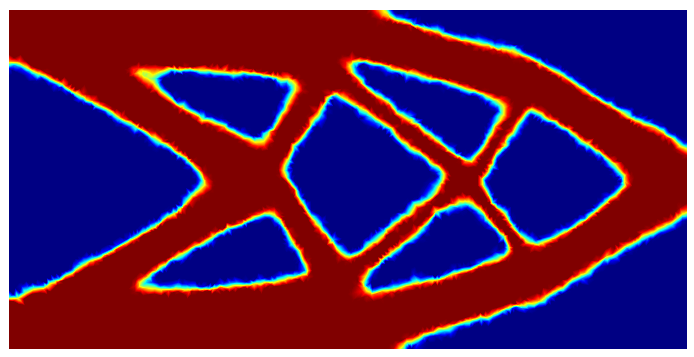
with Young modulus and Poisson’s ratio . Throughout, we fix the penalization parameter . Problem (2.6a)–(2.6b) is solved using the augmented Lagrangian method, in order to handle the volume constraint; see the Augmented Lagrangian method in Algorithm 2. We fix to refine the mesh, and set in the module MARK. The red and blue colors in the design plots below denote the material and void, respectively.
 |
 |
 |
 |
| (a) | (b) | ||
 |
 |
||
| (c) | (d) | (e) | (f) |
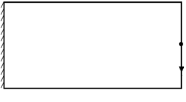
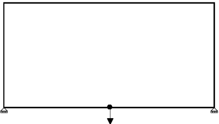
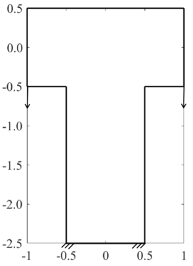
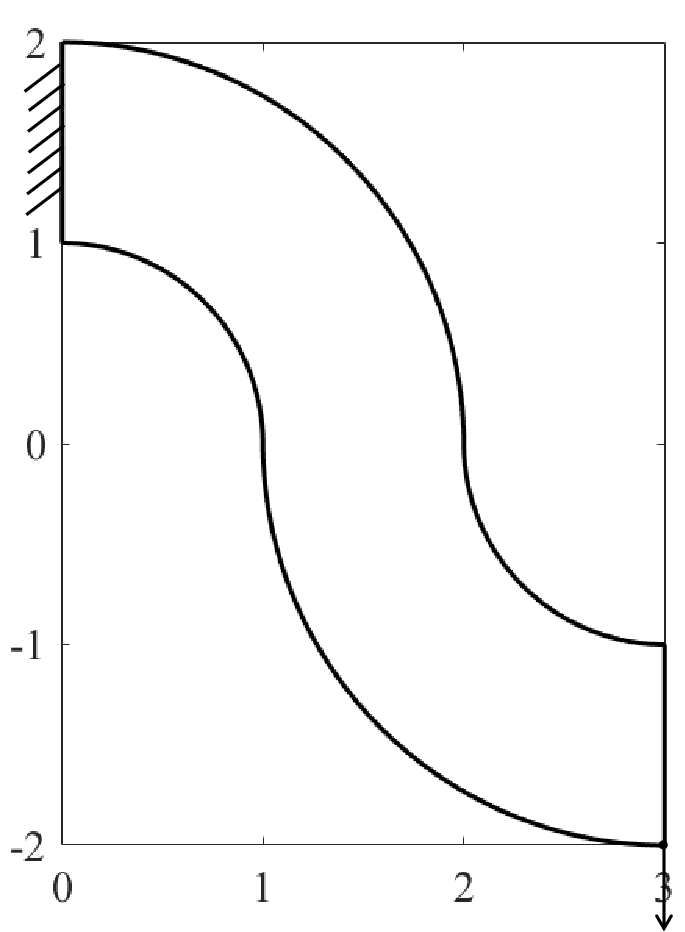
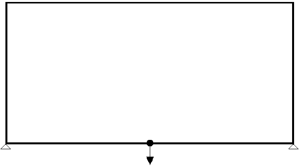
In the numerical experiments, we consider the following six examples. All these examples are very classical in topology optimization. See Fig. 1 for a schematic illustration of the geometry, loading and boundary conditions of the examples.
-
(a)
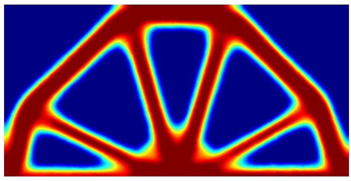
The cantilever problem with the design domain , with . The displacement field on the left side is fixed at zero, and the free traction on the rest except a vertical point load is applied to the middle of the right side.
-
(b)
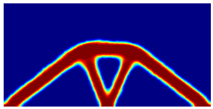
The Messerschmidt-Bolkow-Blohm (MBB) beam problem, with . The settings are identical with (a) except now the low corners are free to move in the -direction and fixed in the -direction, and a unit vertical load is applied in the middle of the lower part and a traction free condition is imposed on the rest.
-
(c)
The cantilever problem as (a), with , except that the low corners are fixed.
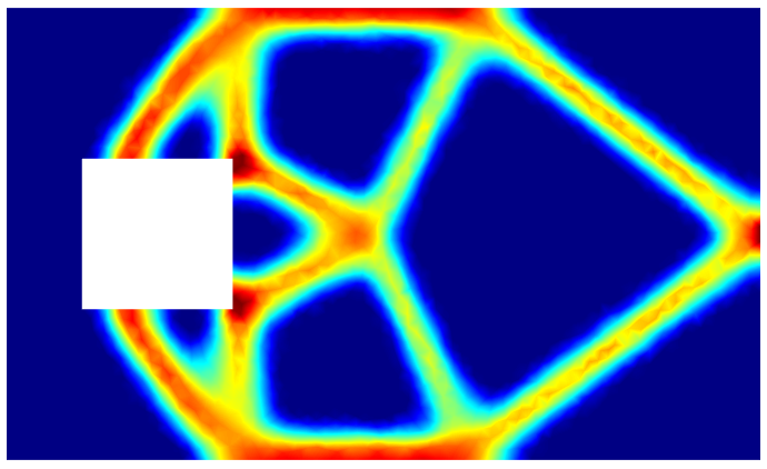
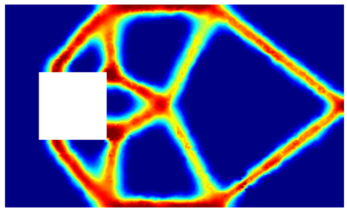
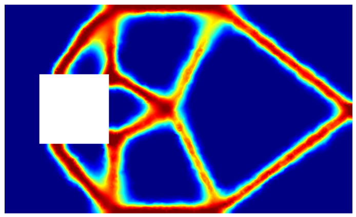
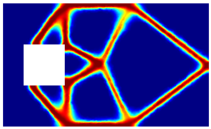
-
(d)
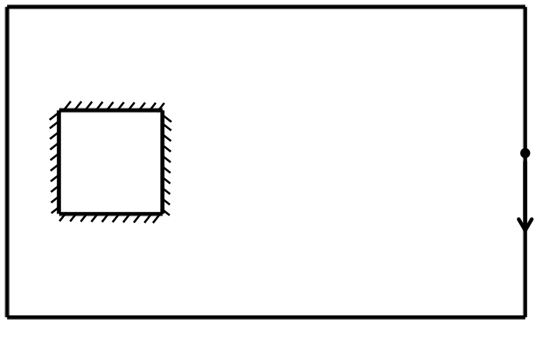
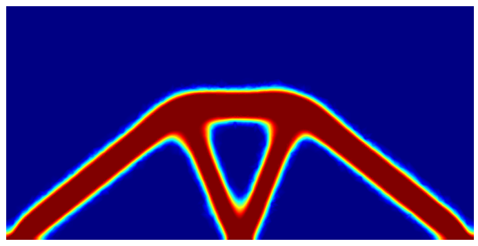
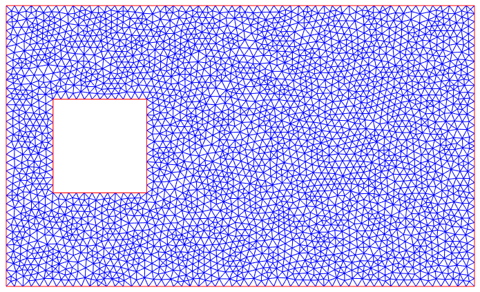
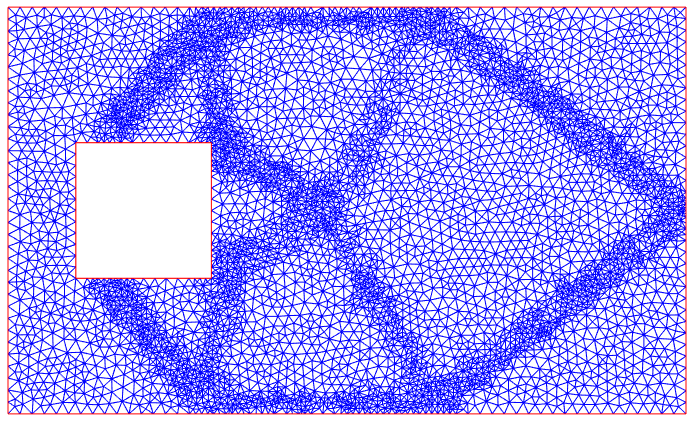
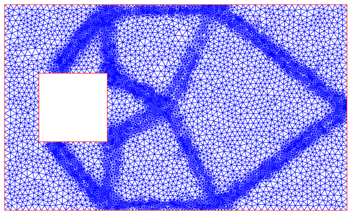
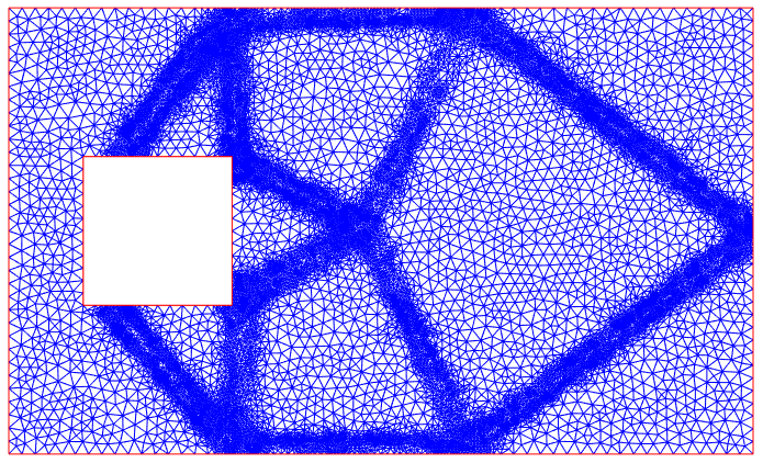
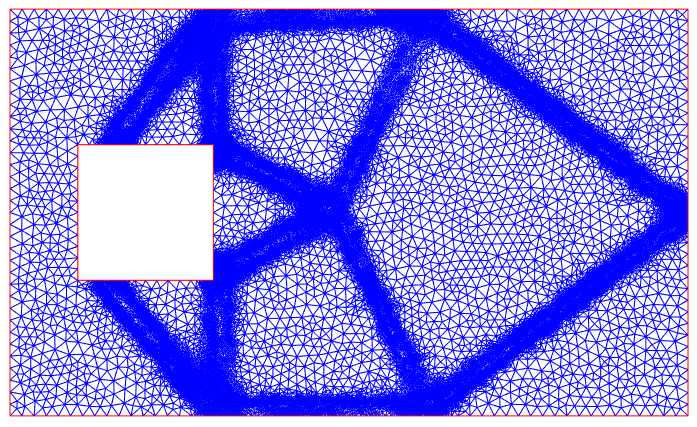
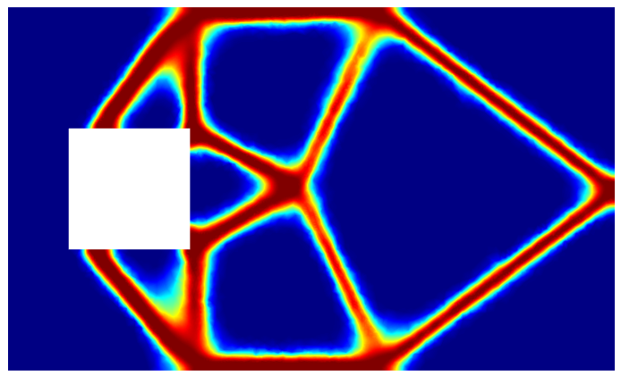
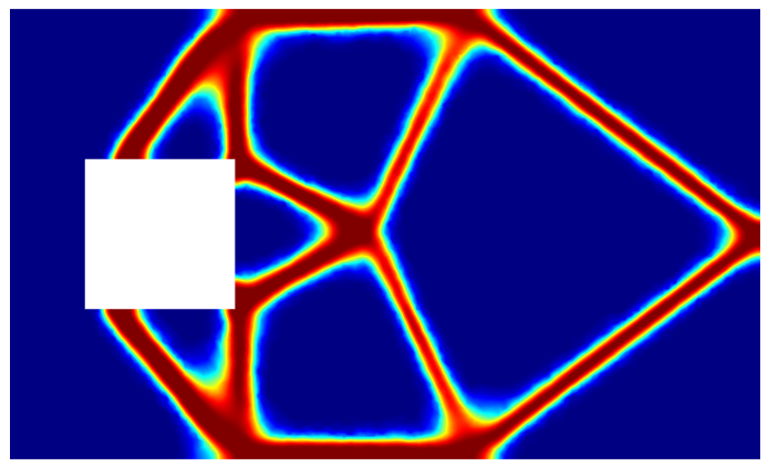
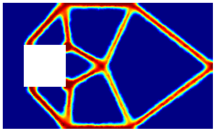
The square hole, the domain , . The inner square boundaries is equipped with a zero Dirichlet boundary condition, and the free traction on the rest except a vertical point load is applied in the middle of the right side.
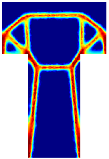
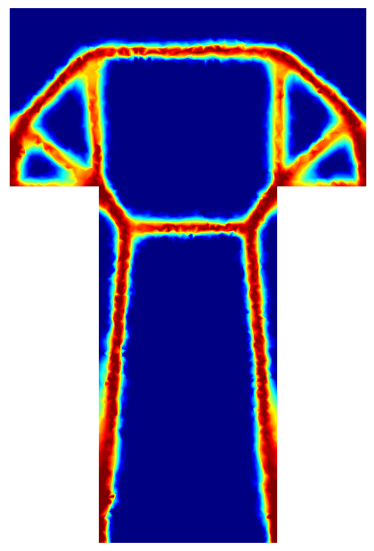
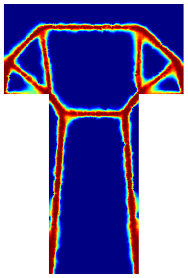
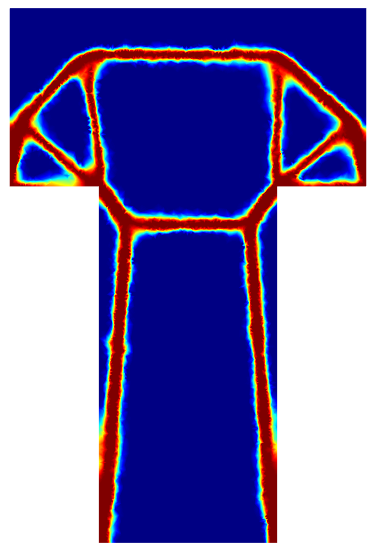
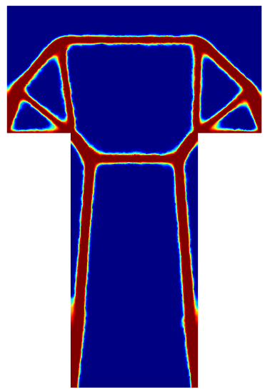
-
(e)
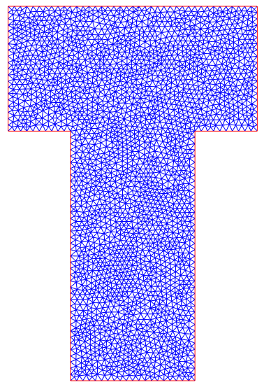
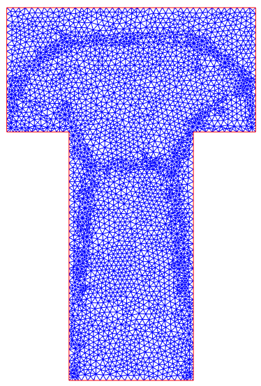
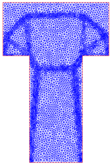
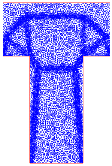
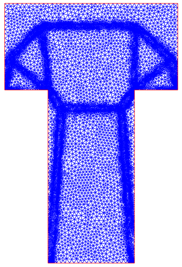
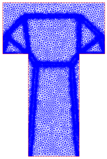
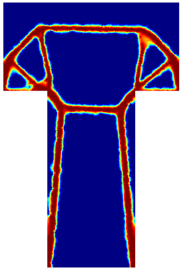
The T-shaped domain with height 3, width 1 at the bottom and 2 at the top, with . The two lower corners are fixed while unit vertical load is applied at the lower corners of the horizontal branch of T.
-
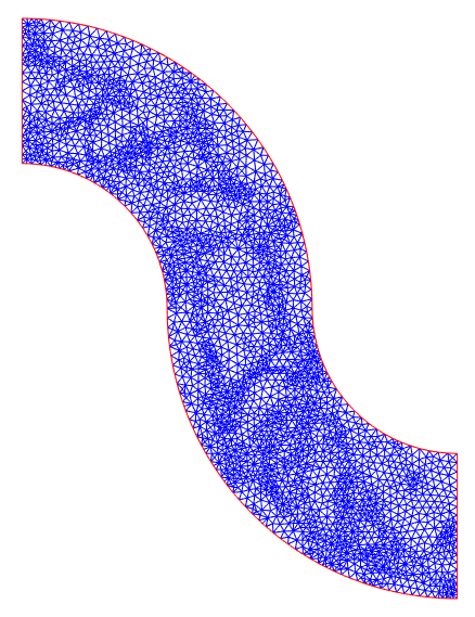
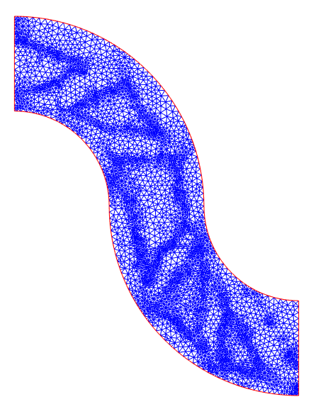
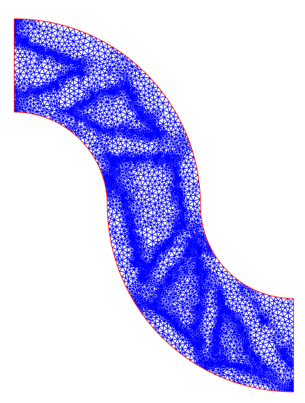
(f)
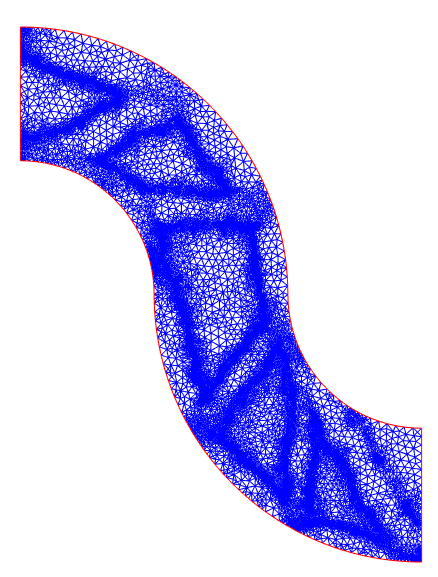
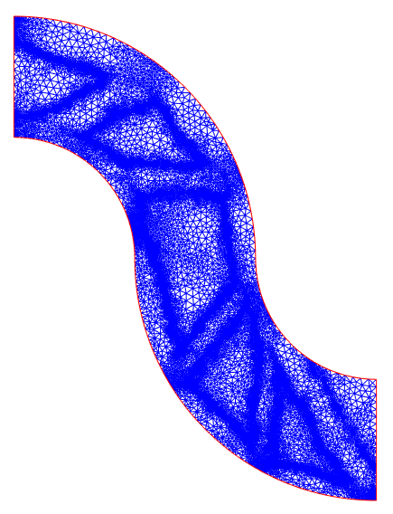
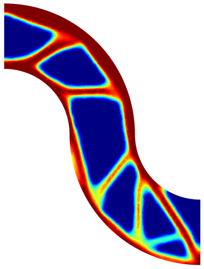
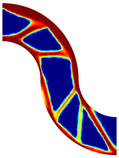
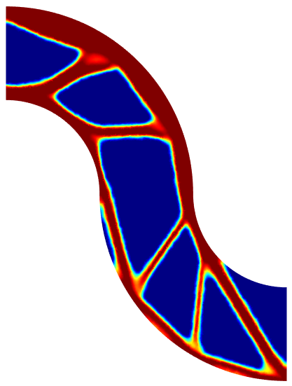
The curved domain, comprising of four arcs and two line segments, and accounts for 40% of the total volume. The left vertical edge is equipped with a zero Dirichlet boundary condition, and the free traction on the rest except a vertical point load is applied in the bottom of the right vertical edge.
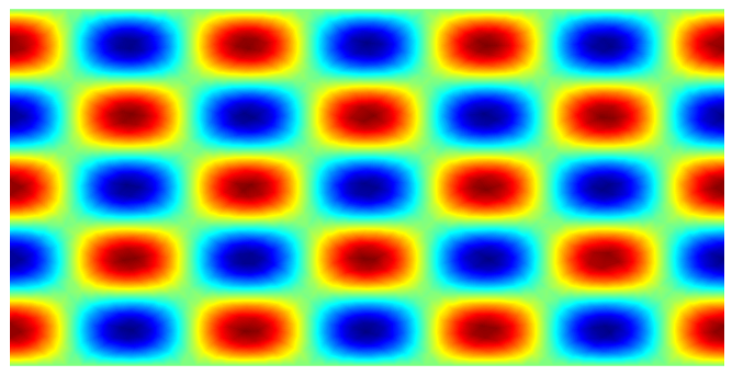
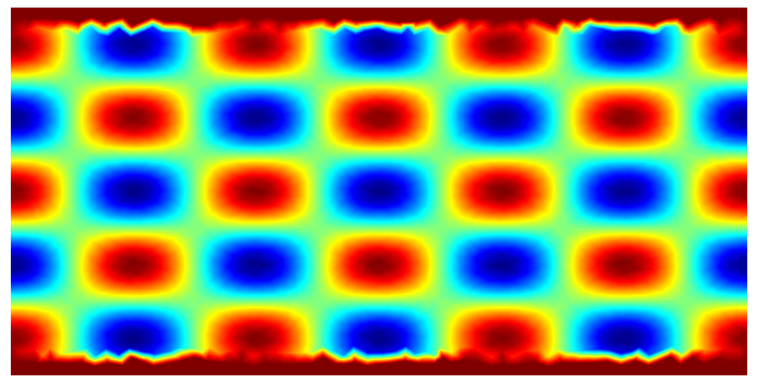
The hyperparameters in Algorithm 2 for the numerical experiments are summarized in Table 1. In the table, denotes the number of (pseudo) time steps for the gradient flow to update the elastic displacement, and denotes the number of inner iterations to update the density field . The scalar is the the phase-field pseudo time step size. The parameters and are the initial Lagrange multiplier, and initial penalty weight for the augmented Lagrangian terms. The two parameters and appear in the phase-field model (2.4a). The lower bound of the density is set to 1e-4 except for Example (d), for which it is set to 1e-3; The factor is fixed at for all examples except for Examples (d) and (e), for which it is set to . In the experiment, the initial phase–field functions for Examples (a)-(c) are shown in Fig. 2, and that for Examples (d)-(f) are taken to be uniform, i.e., 0.3, 0.4 and 0.6, respectively.
| Example | ||||||
|---|---|---|---|---|---|---|
| (a) | 3.5e-2 | 1e-5 | 1e-2 | |||
| (b) | 4.5e-2 | 1e-5 | 1e-2 | |||
| (c) | 4.0e-2 | 5e-5 | 1e-2 | |||
| (d) | 6.5e-3 | 5e-4 | 1e-3 | |||
| (e) | 3.0e-2 | 5e-5 | 1e-2 | |||
| (f) | 2.5e-2 | 5e-5 | 2e-3 |
 |
 |
| Examples (a) and (c) | Example (b) |
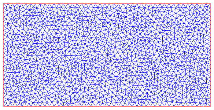
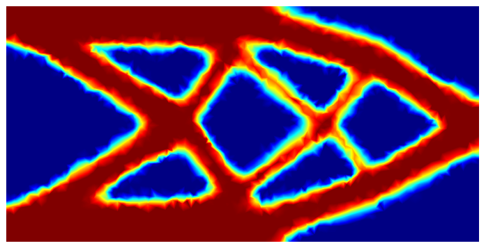
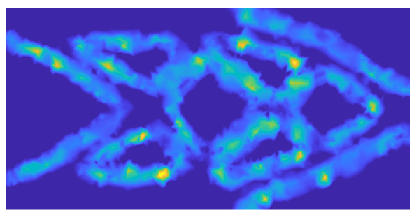
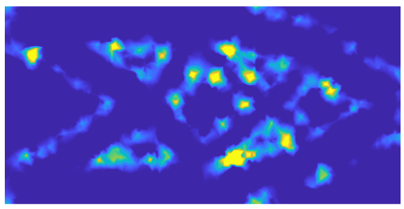
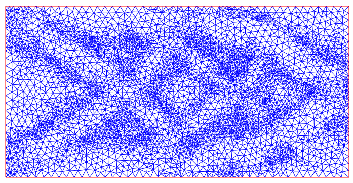
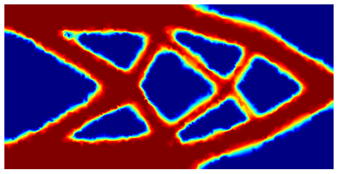
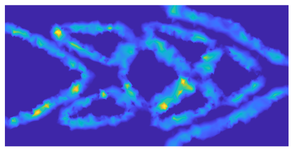
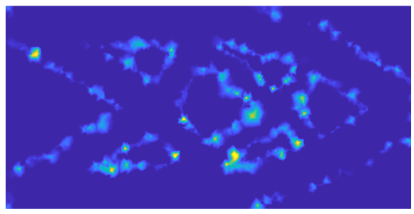
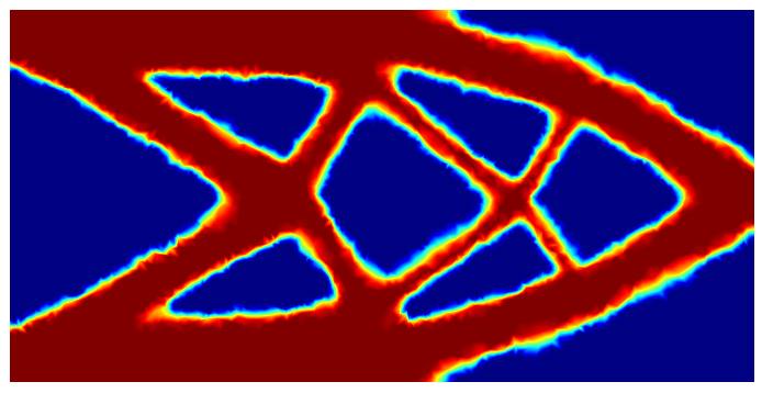
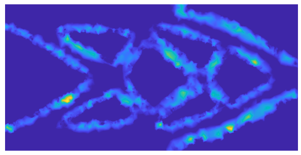
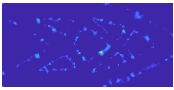
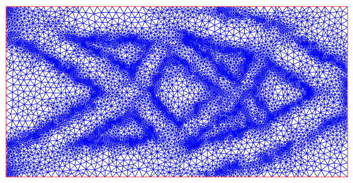
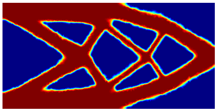
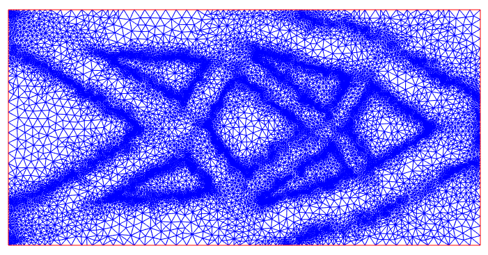
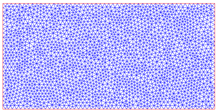
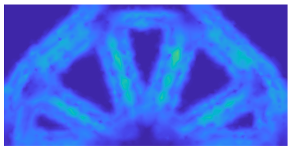
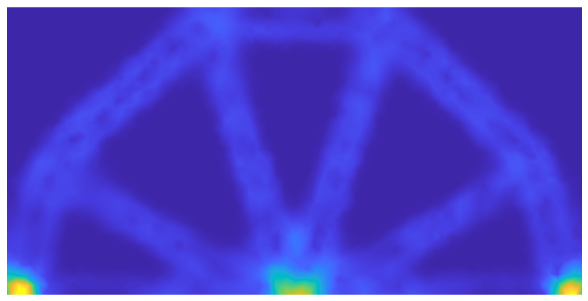
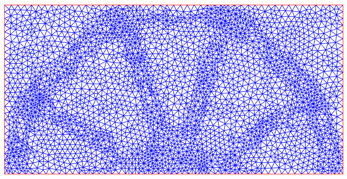
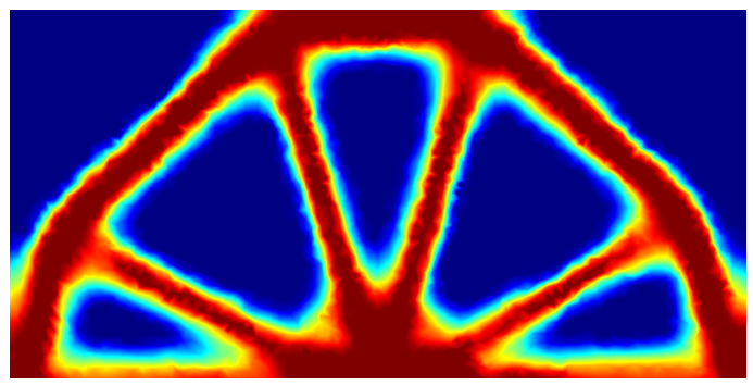
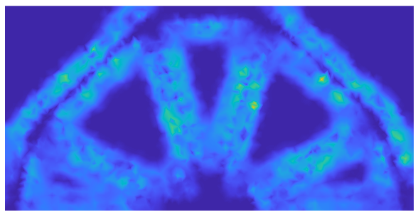
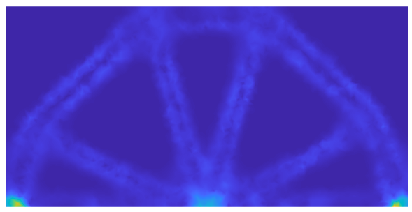
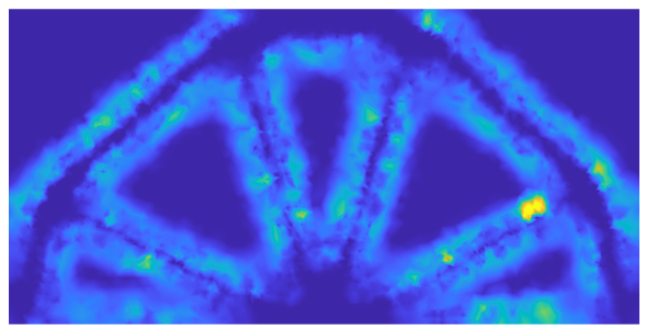
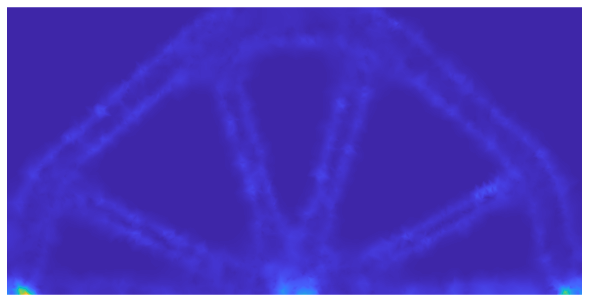
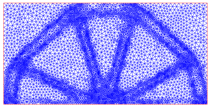
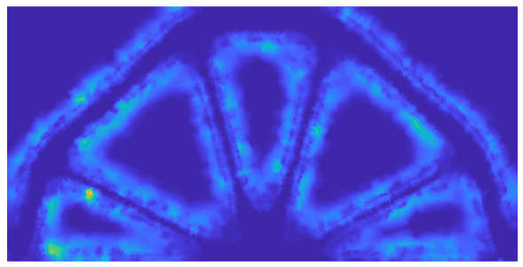
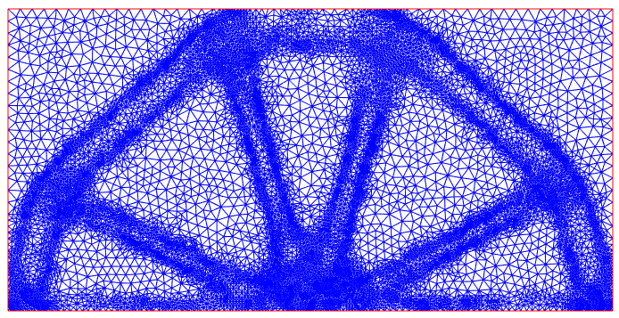
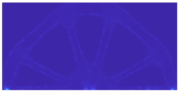
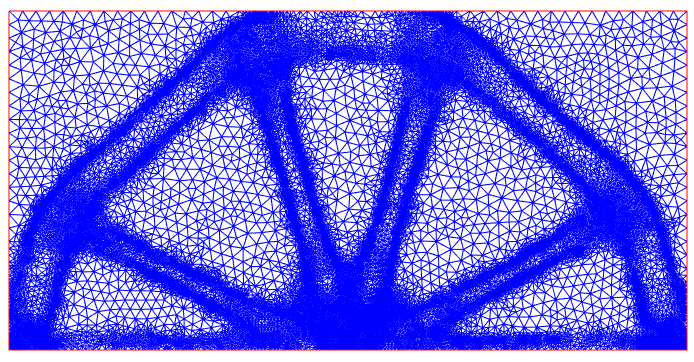
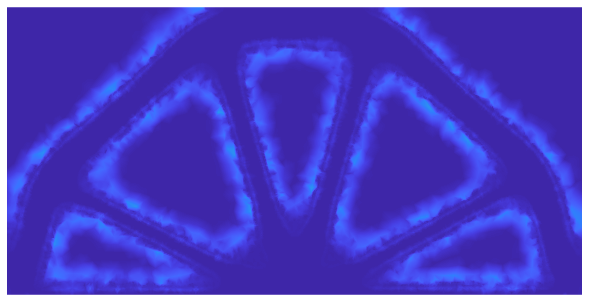
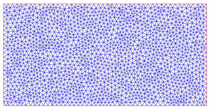
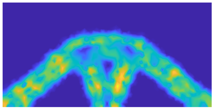
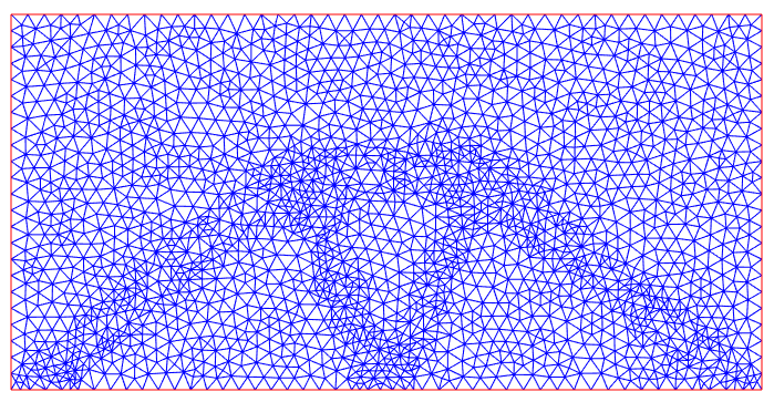
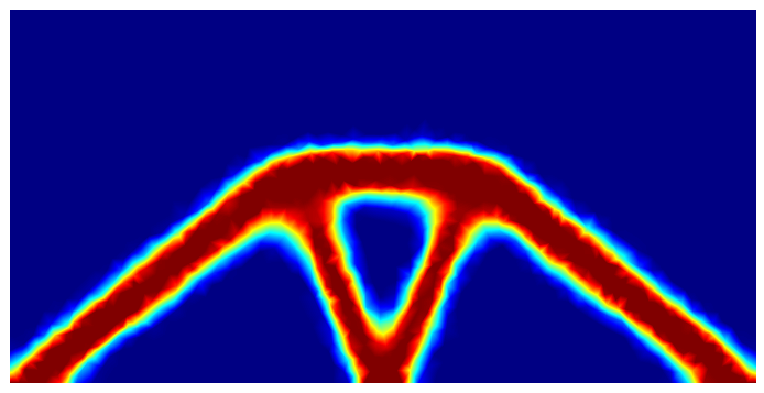
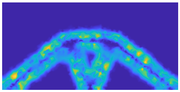
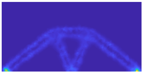
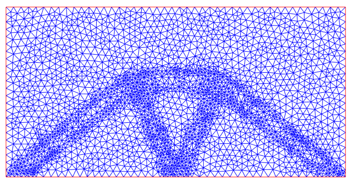
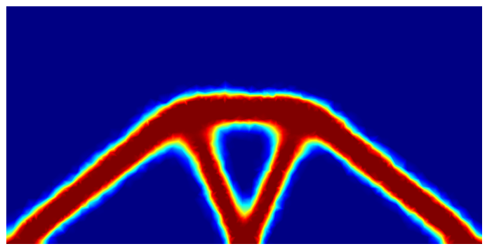
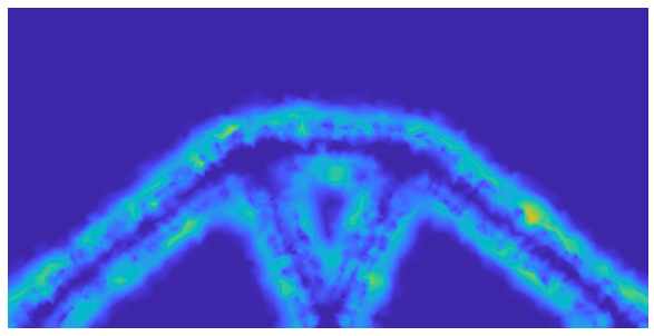
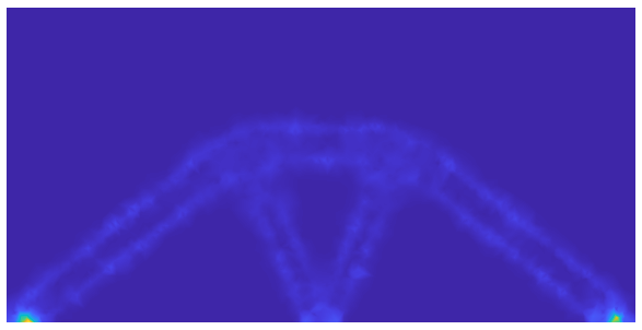
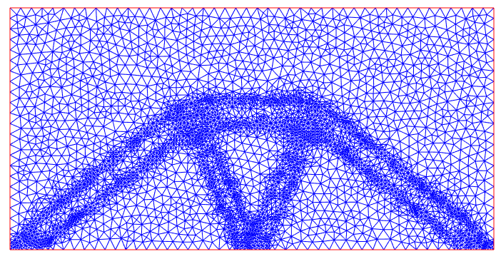
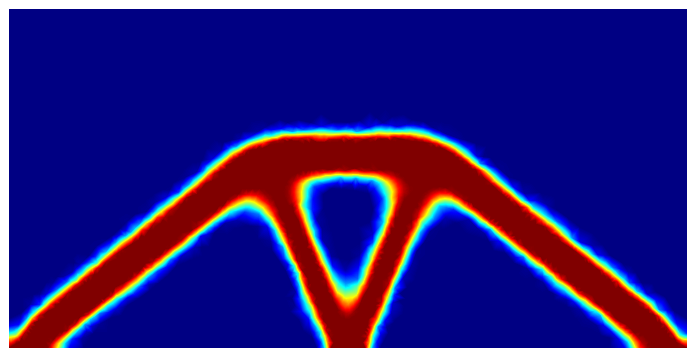
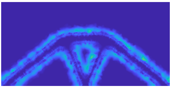
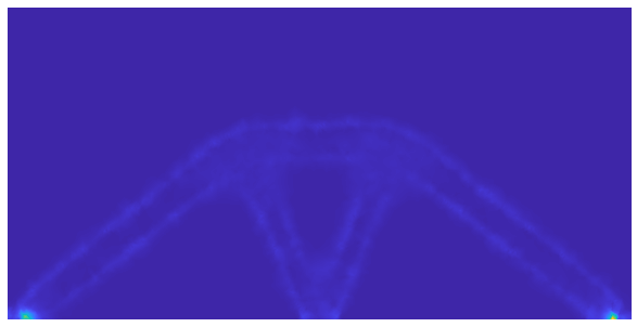
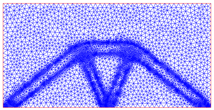
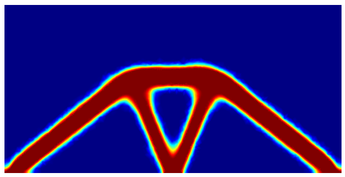
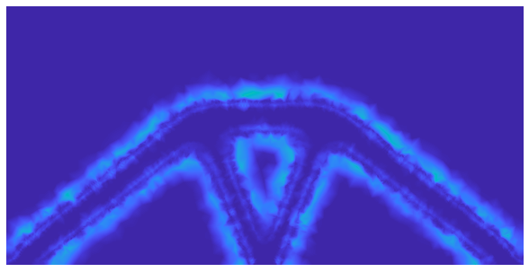
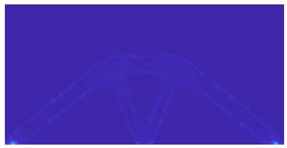
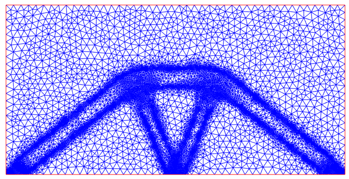
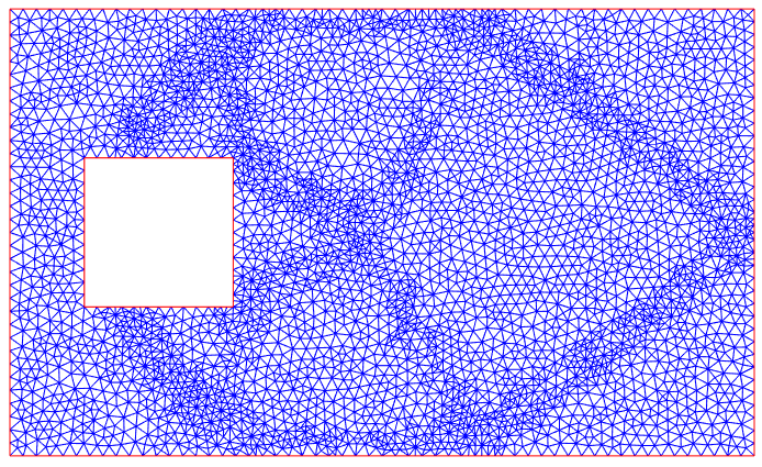
In Figs. 3, 4 and 5, we summarize the results for Examples (a)–(c), including the evolution of meshes, optimal design and the error estimates during the adaptive refinement process. It is observed that as the adaptive loop proceeds, Algorithm 1 can accurately capture interfaces between the material and the void regions, around which local refinements are performed. More precisely, the first adaptive iterations yield a rough topology of the desired design, and with the subsequent adaptive refinement, the algorithm produces improved boundary interfaces of the solid material, due to the better resolution of the state variable . Notably, the additional refinements mainly take place around the interfaces during the adaptive refinement procedure, which shows clearly the effectiveness of the proposed adaptive algorithm. These observations hold also Example (d)–(f); see Figs. 6, 7 and 8 for the evolution of the mesh and optimal design during the adaptive refinement process.
 |
 |
 |
 |
 |
 |
 |
 |
 |
 |
 |
 |
 |
 |
 |
 |
 |
 |
 |
 |
 |
 |
 |
 |
 |
 |
 |
 |
 |
 |
 |
 |
 |
 |
 |
 |
 |
 |
 |
 |
 |
 |
 |
 |
 |
 |
 |
 |
 |
 |
 |
 |
 |
 |
 |
 |
 |
 |
 |
 |
 |
 |
 |
 |
 |
 |
 |
 |
 |
 |
 |
 |
 |
 |
 |
 |
 |
 |
 |
 |
 |
 |
 |
 |
 |
 |
 |
 |
 |
 |
 |
 |
 |
 |
 |
 |

|
 |
 |
 |
 |
 |
 |
 |
 |
 |
 |
 |
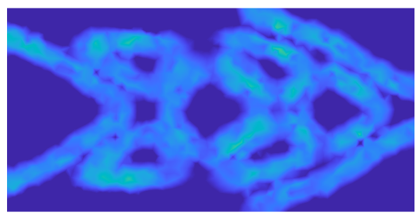
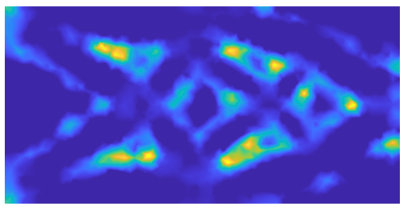
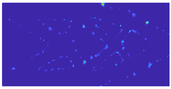
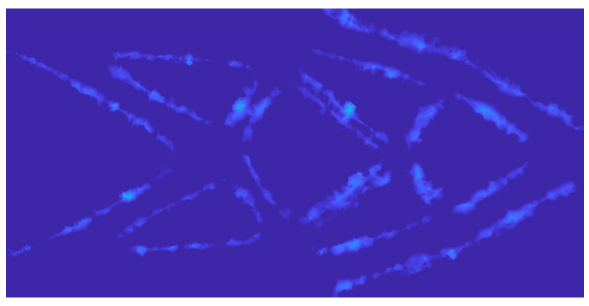
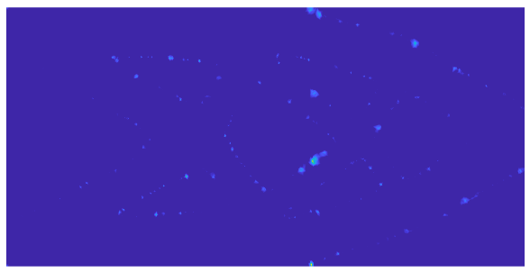
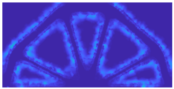
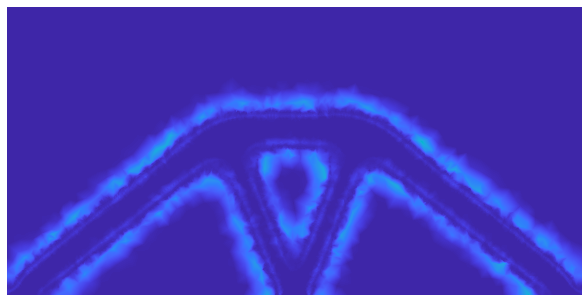
In Figs. 3, 4 and 5, we show also the evolution of the error estimators and for Examples (a)–(c). By the very construction, the two estimators and play different roles: indicates the presence of the design edges, whereas concentrates on the variation of the displacement field . The magnitude of is observed to be much smaller than for all three examples (and also for the remaining examples, although not shown). The precise mechanism for this interesting phenomenon is still unknown. Nonetheless, this observation clearly indicates that one may only use as the error indicator to drive the adaptive procedure in practical computation. Also it is observed that the magnitudes of the estimators decreases steadily to zero throughout the adaptive process, concurring with the vanishing property numerically, cf. Lemma 5.2.
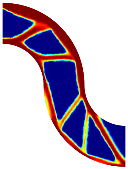
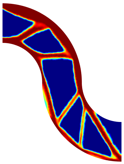
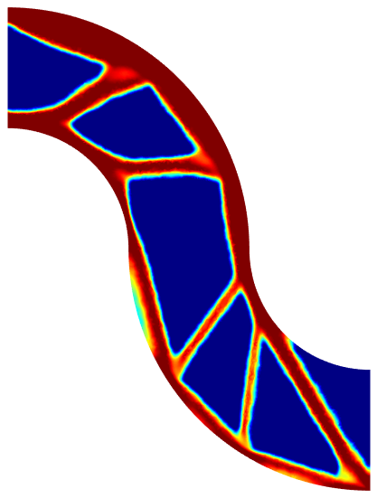
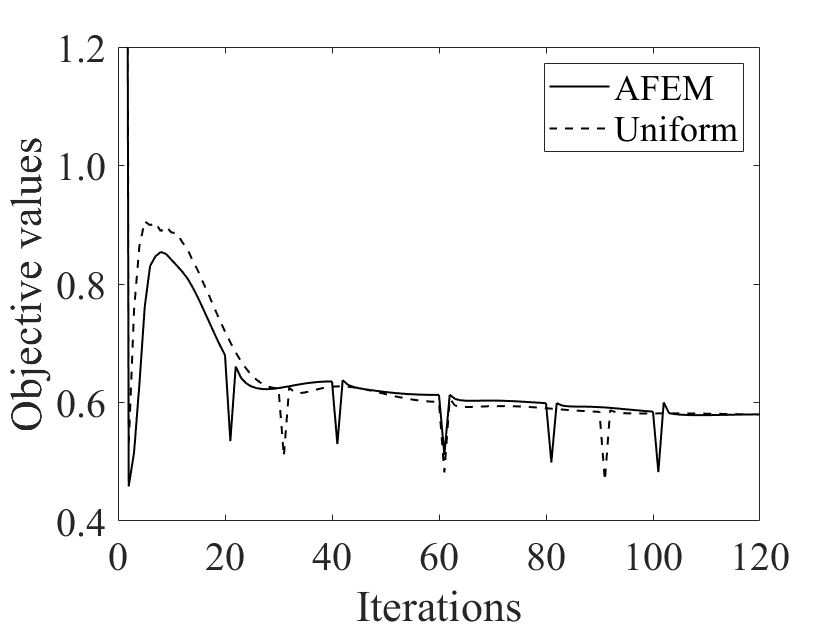
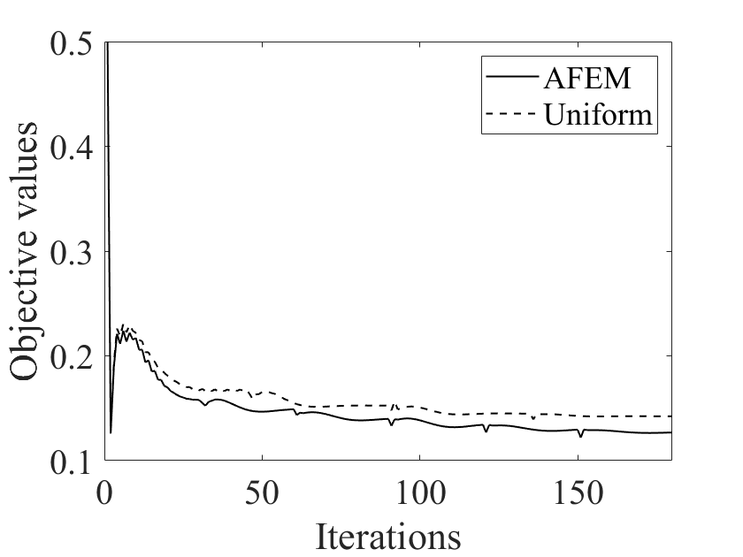
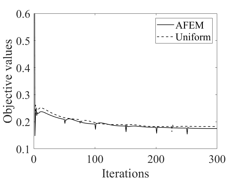
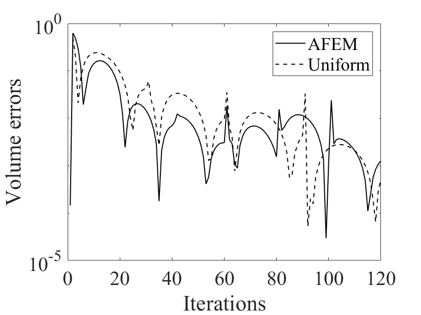
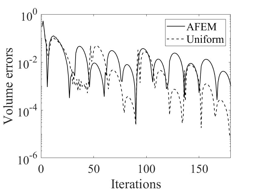
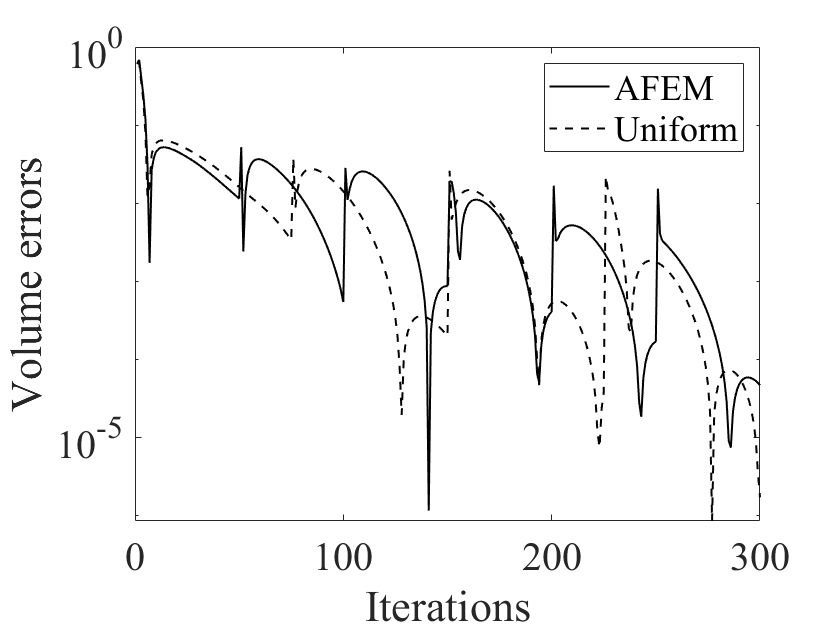
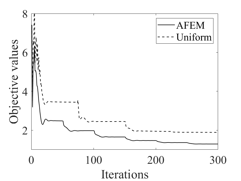
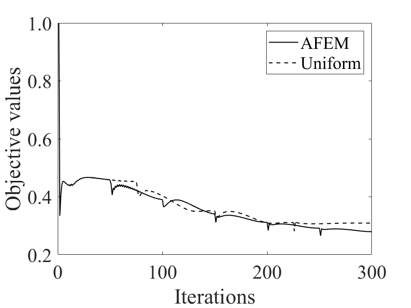
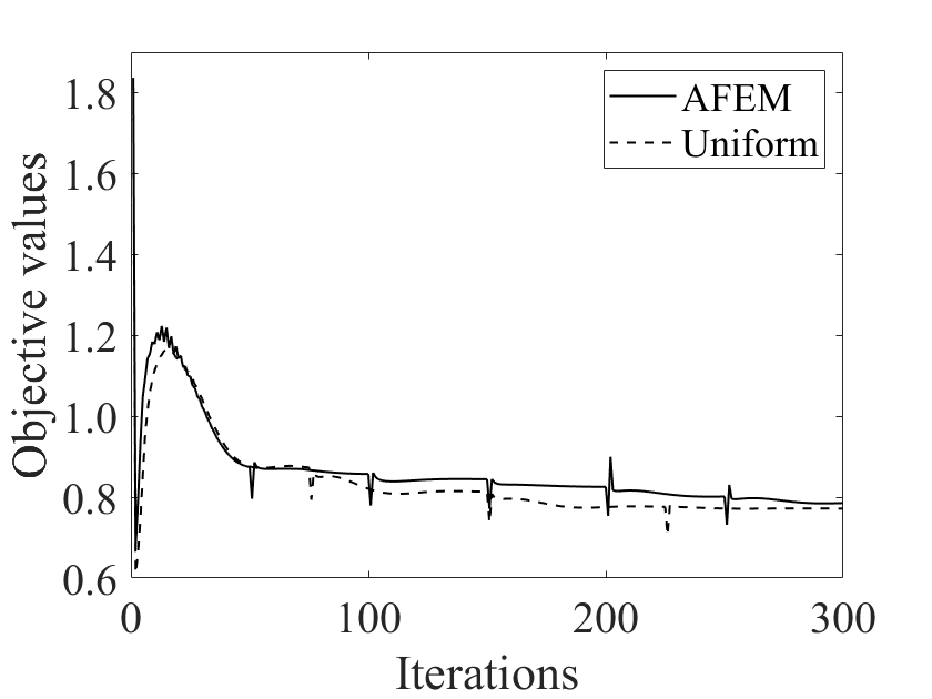
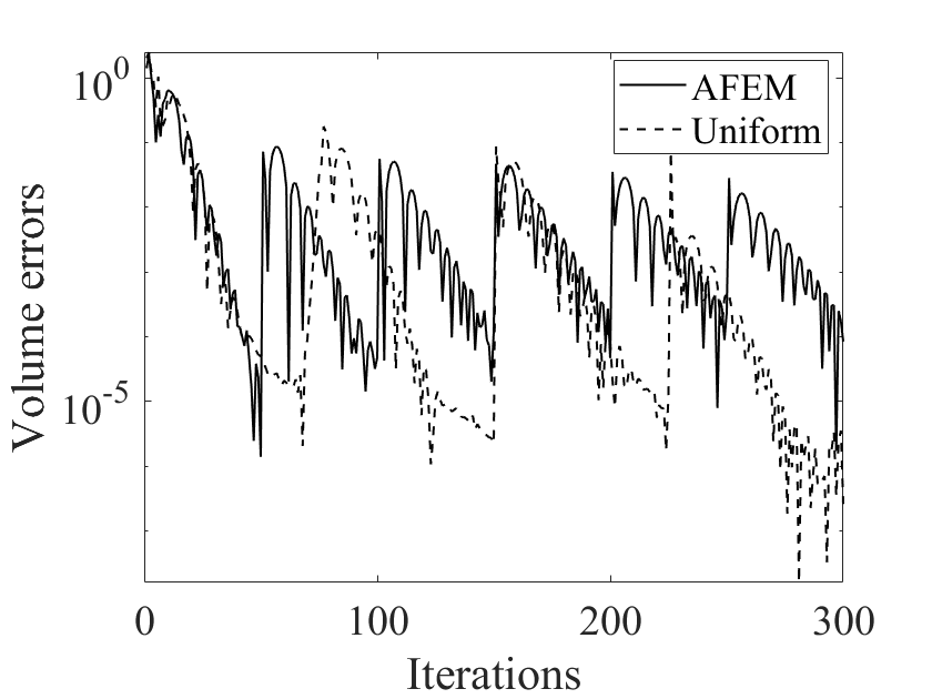
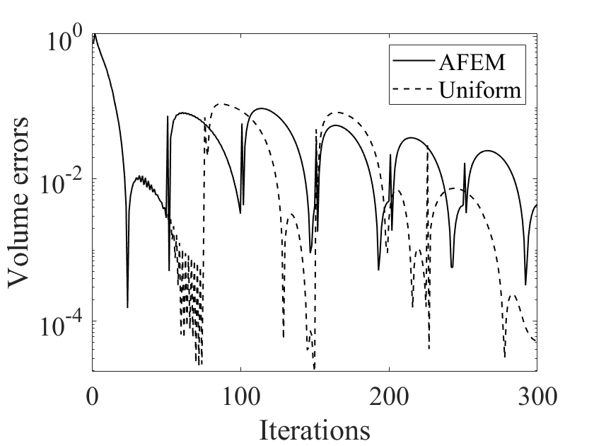
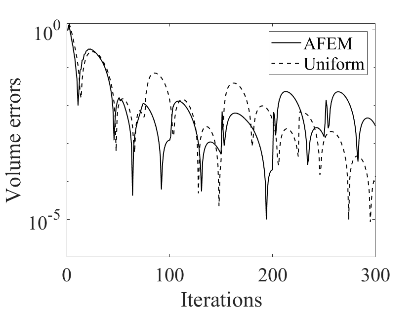
The use of the adaptive algorithm does influence also the performance of Algorithm 2. In Fig. 9, we compare the decay of the objective value and the volume error by the adaptive and uniform refinements, where the refinement steps and iteration numbers of the augmented Lagrangian method for adaptive and uniform refinements are adjusted such that the total numbers of iterations and the numbers of vertices on the final meshes are comparable. It is observed that for both refinement strategies, the objective values perform equally well, and the volume constraint is well preserved during the refinement process by both strategies. Also it is consistently observed that at the beginning of the iteration, the objective value decreases rapidly, and then it stabilizes. In particular, the final objective values are always very close to each other for both refinement strategies, which agree with the fact that converged optimal designs are visually similar, cf. Fig. 10.
 |
 |
 |
 |
 |
 |
| (a) | (b) | (c) |
 |
 |
 |
 |
 |
 |
| (d) | (e) | (f) |
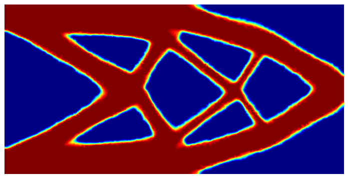
Table 2 presents more quantitative results for both refinement strategies: the values of the objective functional (achieved at the final meshes generated by the uniform and adaptive refinements), the number of vertices on the final mesh, and the computing time (in seconds). Interestingly, the objective functional for the adaptive refinement is very close to the uniform one, or slightly smaller. Moreover, the computing time is comparable: the adaptive algorithm saves between 20% and 50% of the time compared to the uniform refinement. Fig. 10 shows the optimized designs of the two methods and it can be seen that the boundary of adaptive algorithm is smoother, with less small oscillations along the interfaces, than that by the uniform refinement. This is attributed to the better resolution of the interface and the displacement field by the adaptive strategy.
| adaptive | uniform | ||||||
|---|---|---|---|---|---|---|---|
| Example | vertices | objective | time (sec) | vertices | objective | time (sec) | saving |
| (a) | 16080 | 0.5800 | 1216.19 | 16080 | 0.5798 | 1496.36 | 18.72% |
| (b) | 22618 | 0.1269 | 3599.94 | 22434 | 0.1423 | 4758.11 | 24.34% |
| (c) | 10035 | 0.1750 | 1089.00 | 9948 | 0.1826 | 2142.86 | 49.19% |
| (d) | 24063 | 1.2917 | 6251.19 | 23987 | 1.8893 | 10586.30 | 40.95% |
| (e) | 18425 | 0.2796 | 3963.81 | 18552 | 0.3090 | 7716.75 | 48.63% |
| (f) | 25542 | 0.7855 | 8816.58 | 25548 | 0.7719 | 13264.08 | 33.53% |
| (a) | (b) | ||
|
 |
|
 |
| (c) | (d) | ||
|
 |
|
 |
| (e) | (f) | ||
|
 |
|
 |
5 Convergence analysis
Now we analyze the convergence of Algorithm 1. First, we introduce an auxiliary minimum compliance problem over a limiting admissible set given by Algorithm 1 (cf. (5.1a) below). Then using techniques in nonlinear optimization, the sequence of adaptively generated solutions is shown to contain a subsequence convergent to the solution of the auxiliary problem in . Then the desired result follows by proving that the solution also satisfies the necessary optimality system (2.5). Note that two error indicators and are involved in Algorithm 1, however, in the process of our analysis, only one subsequence convergence is obtained.
The convergence analysis employs the following auxiliary problem:
| (5.1a) | |||
| (5.1b) | |||
where and are closures of given by Algorithm 1, i.e.,
Lemma 5.1.
is a closed subspace of and is a closed convex subset of .
Proof.
By definition, (respectively ) is closed in (respectively ). For any and in , there exist two sequences and such that and in . By the convexity of the set , for any . Then in , i.e. for any since is closed. Hence is convex. Moreover, we have and almost everywhere in after (possibly) passing to a subsequence, which, along with the constraint and almost everywhere in , indicates that and almost everywhere in . Lastly, the fact that implies . ∎
Theorem 5.1.
Proof.
Since the constant function for all , the minimizing property of over and the stability (2.7) for the associated discrete displacement field imply that
The box constraint in implies that , and thus is uniformly bounded in . By Lemma 5.1 and Sobolev embedding theorem, there exist a subsequence, denoted by , and some such that
| (5.2) |
Next we define a discrete analogue of the variational problem in (5.1a) with : find such that
| (5.3) |
That is, is the finite element approximation of the solution to the auxiliary problem (5.1b)) (with the constraint with ). By Korn’s inequality, Céa’s lemma and the density of in , we have
| (5.4) |
Meanwhile, taking in (5.3) and (2.6b) yields
By the pointwise convergence in (5.2) and Lebesgue’s dominated convergence theorem [23, Theorem 1.19], we get
which, together with the inequality and Korn’s inequality, implies . This, (5.4), and the triangle inequality show
| (5.5) |
Since solves (2.6b) with and solves (5.1b) with , it follows from (5.5) that
| (5.6) | ||||
Using the pointwise convergence in (5.2) and Lebesgue’s dominated convergence theorem again gives
| (5.7) |
Now, for any there exists a sequence such that in . Using the above argument and a standard subsequence argument gives
Now combining (5.6) with (5.7), the weak lower semicontinuity of -seminorm and the minimizing property of to over , we get
Since , is a minimizer of over . Moreover, taking in the last inequality, we obtain
It follows from (5.6) and (5.7) that
This directly implies in , and completes the proof of the theorem. ∎
In view of Theorem 5.1, it suffices to prove that the tuple satisfies (2.5). We make use of the marking strategy (3.4)-(3.5). In the proof, we denote by the union of all elements in with a non-empty intersection with an element and by the union of elements in sharing a common edge with .
Lemma 5.2.
Proof.
We relabel as . Since the module MARK in Algorithm 1 involves comparing two estimators and , the convergent subsequence consists of two subsequences (relabeled as) and with
| (5.9) |
| (5.10) |
Next we divide the lengthy proof into three steps.
Step 1. For any and any , Young’s inequality implies that
| (5.11) | ||||
Since is an integer, is a polynomial of degree over . By the element inverse estimates for finite element functions,
and by the scaled trace theorem [47] and the element inverse estimate, we deduce
Summing the estimate (5.11) over all elements and using the last two estimates and the finite overlapping property of the neighborhood give
| (5.12) |
Next we bound the terms separately. By Theorem 5.1, and Lebesgue’s dominated convergence theorem, we deduce
| (5.13) |
For the last term, by the triangle inequality, we have
It follows from Theorem 5.1 that the sequence is uniformly bounded. Then by the symmetry of the tensor and the Cauchy-Schwarz inequality,
Similarly,
Upon noting the pointwise convergence of in Theorem 5.1 and , and applying Lebesgue’s dominated convergence theorem, we find
The last three vanishing limits imply
| (5.14) |
Meanwhile, any is generated by applying bisection to some at least once. Thus and is zero across a side in the interior of . Therefore, we can split the term in (5.12) as
which, along with and Dörfler marking criterion (3.4), yields
| (5.15) |
Now collecting the estimates (5.12)–(5.15) leads to
where for a sufficiently small ,
and
Therefore, one can prove that (cf. [2, Lemma 2.3])
Then due to the condition (5.9), we have
i.e., the desired vanishing limits hold for .
Step 2. For the sequence , by Young’s inequality, we derive that for any and any
Since each component of and is a constant and is also a polynomial of degree on any , as previously in Step 1, we obtain
and by the scaled trace theorem [47] and the inverse estimate,
Consequently,
| (5.16) |
By Dörfler marking criterion (3.5) and repeating the argument for (5.15), we obtain
| (5.17) |
By the triangle inequality,
Since and are both uniformly bounded due to Theorem 5.1, the Cauchy-Schwarz inequality implies
Likewise,
By appealing to Theorem 5.1 again, we deduce
Lebesgue’s dominated convergence theorem implies
Therefore,
| (5.18) |
Repeating the preceding argument yields
| (5.19) |
It follows from (5.16)–(5.19) that
where for sufficiently small ,
and
Like before, we obtain
Then by the condition (5.10), we have
Step 3. Since and comprise , the vanishing limits obtained in Steps 1 and 2 for the two subsequences ensure the desired identity (5.8). ∎
The next result gives the asymptotic vanishing property (of the residual operators).
Lemma 5.3.
To prove Lemma 5.3, we need a constraint-preserving interpolation operator for -functions introduced in [29]. Let be the set of all nodes of and be the nodal basis functions in . For each , the support of is denoted by , i.e., the union of all elements in with being a vertex, and is the triangulation of with respect to . Then we define an interpolation operator by
| (5.22) |
It follows from the definition (5.22) that
| (5.23) |
Further, by the standard trapezoidal rule,
So preserves the integral constraint in , i.e.,
| (5.24) |
Moreover, there hold the following stability and error estimates [29, Lemma 5.3].
Lemma 5.4.
For all on all and any , there hold
| (5.25) |
| (5.26) |
Proof of Lemma 5.3.
Like before, we relabel the convergent subsequence as . The basic idea of the proof has been described when motivating the two estimators in Section 3. Below we expand the idea rigorously. Since is a minimizer to problem (2.6a)–(2.6b) over the triangulation , it satisfies the following discrete variational inequality (see the first variational inequality of (3.3)):
| (5.27) |
Due to the conservation properties (5.23)–(5.24), there holds for any . Letting in (5.27) gives that for any ,
| (5.28) |
By elementwise integration by parts, the Cauchy-Schwarz inequality, the definition of the error indicator and error estimates for from Lemma 5.4, we get
Now the assertion (5.20) follows from (5.28) and Lemma 5.2. The proof of (5.21) is similar. On the space , we define a vectorial operator with each component being the Scott-Zhang quasi-interpolation [40]. Since solves (2.6b), by applying the operator to any , elementwise integration by parts and using the definition of , error estimates for [40] and the Cauchy-Schwarz inequality, we obtain that for any ,
Remark 5.1.
Lemma 5.5.
Proof.
We relabel the convergent subsequence in Theorem 5.1 as . In view of the -convergence of from Theorem 5.1, we have
| (5.30) |
Since , by the pointwise convergence of and Lebesgue’s dominated convergence theorem [23, Theorem 1.19],
| (5.31) |
Direct computation yields for any ,
Due to , the -convergence of to in Theorem 5.1 implies
Since , the pointwise convergence of and Lebesgue’s dominated convergence theorem [23, Theorem 1.19] imply
Collecting the last three estimates leads to
| (5.32) |
By invoking (2.6b) with and (5.1b) with and arguing as for (5.6) (see the proof of Theorem 5.1), we further have
| (5.33) | ||||
Then it follows from (5.30)-(5.33) and (5.20) in Lemma 5.3 that
For the variational problem in (5.29), Theorem 5.1 and the dominated convergence imply
Therefore,
This and (5.21) in Lemma 5.3 imply the desired variational equation, which completes the proof of the lemma. ∎
Remark 5.2.
In the convergence analysis, we have assumed that in the tensor is an integer. This assumption is only used in the proof of Lemma 5.2. The rest of convergence analysis does not rely on this assumption.
6 Conclusions
In this work we have developed a novel adaptive phase-field approximation for compliance optimization, one fundamental problem in topology optimization. The approach is based on the phase-field representation of the medium (material versus void), and adaptive finite element discretization of the phase-field function and the displacement field. The estimators driving the adaptive refinement procedure consist of two parts: one for the objective functional (and the first-order necessary condition), and the other for the displacement field approximation. We provided a convergence analysis of the approximation in the sense that the sequence of the optimal states and designs contains a convergent subsequence to a solution of the first-order necessary optimality system. Furthermore, we presented numerical experiments which show clearly the accuracy and efficiency of the proposed adaptive phase-field approach. It is observed that the adaptive approach can yield optimal designs with comparable objective values but sharper and smoother interfaces at a lower computational cost, and hence it has significant potential for topology optimization.
References
- [1] M. Ainsworth and J. T. Oden. A Posteriori Error Estimation in Finite Element Analysis. Pure and Applied Mathematics. Wiley-Interscience, John Wiley & Sons, New York, 2000.
- [2] M. Aurada, S. Ferraz-Leite, and D. Praetorius. Estimator reduction and convergence of adaptive BEM. Appl. Num. Math., 62:787–801, 2012.
- [3] M. P. Bendsøe. Optimal shape design as a material distribution problem. Struct. Opt., 1(4):193–202, 1989.
- [4] M. P. Bendsøe and N. Kikuchi. Generating optimal topologies in structural design using a homogenization method. Comput. Methods Appl. Mech. Engrg., 71(2):197–224, 1988.
- [5] M. P. Bendsøe and O. Sigmund. Material interpolation schemes in topology optimization. Arch. Appl. Mech., 69(9–10):635–645, 1999.
- [6] M. P. Bendsøe and O. Sigmund. Topology Optimization: Theory, Methods and Applications. Springer-Verlag, Berlin, 2003.
- [7] L. Blank, H. Garcke, C. Hecht, and C. Rupprecht. Sharp interface limit for a phase field model in structural optimization. SIAM J. Control Optim., 54(3):1558–1584, 2016.
- [8] B. Bourdin and A. Chambolle. Design-dependent loads in topology optimization. ESAIM Control Optim. Calc. Var., 9:19–48, 2003.
- [9] B. Bourdin and A. Chambolle. The phase-field method in optimal design. In M. P. Bendsøe, N. Olhoff, and O. Sigmund, editors, IUTAM Symposium on Topological Design Optimization of Structures, Machines and Materials, pages 207–215. Springer, Berlin, 2006.
- [10] D. Braess. Finite Elements: Theory, Fast Solvers, and Applications in Elasticity Theory. Cambridge University Press, Cambridge, third edition, 2007.
- [11] S. C. Brenner and L. R. Scott. The Mathematical Theory of Finite Element Methods. Springer, New York, third edition, 2008.
- [12] M. Bruggi and M. Verani. A fully adaptive topology optimization algorithm with goal-oriented error control. Comput. Struct., 89(15–16):1481–1493, 2011.
- [13] M. Burger and R. Stainko. Phase-field relaxation of topology optimization with local stress constraints. SIAM J. Control Optim., 45(4):1447–1466, 2006.
- [14] J. Cahn and J. Hilliard. Free energy of a non-uniform system i–interfacial free energy. J. Chem. Phys., 28(2):258–267, 1958.
- [15] P. G. Ciarlet. The Finite Element Method for Elliptic Problems. SIAM, Philadelphia, PA, 2002.
- [16] P. G. Ciarlet. Linear and Nonlinear Functional Analysis with Applications. SIAM, Philadelphia, PA, 2013.
- [17] J. C. A. Costa Jr and M. K. Alves. Layout optimization with –adaptivity of structures. Int. J. Numer. Method Eng., 58(1):83–102, 2003.
- [18] E. de Sturler, G. H. Paulino, and S. Wang. Topology optimization with adaptive mesh refinement. In J. F. Abel and J. R. Cooke, editors, Proceedings of the Sixth International Conference on Computation of Shell and Spatial Structures IASS-IACM 2008: Spanning Nano to Mega, Ithaca, NY, USA, 2008.
- [19] M. A. S. de Troya and D. A. Tortorelli. Adaptive mesh refinement in stress-constrained topology optimization. Struct. Multidisc. Optim., 58(6):2369–2386, 2018.
- [20] L. Dedè, M. J. Borden, and T. J. R. Hughes. Isogeometric analysis for topology optimization with a phase field model. Arch. Comput. Methods Eng., 19(3):427–465, 2012.
- [21] A. Díaz and O. Sigmund. Checkerboard patterns in layout optimization. Struct. Optim., 10(1):40–45, 1995.
- [22] H. A. Eschenauer and N. Olhoff. Topology optimization of continuum structures: A review. Appl. Mech. Rev., 54(4):331–390, 2001.
- [23] L. C. Evans and R. F. Gariepy. Measure Theory and Fine Properties of Functions. CRC Press, Boca Raton, FL, revised edition, 2015.
- [24] C. Fleury. CONLIN: an efficient dual optimizer based on convex approximation concepts. Struct. Optim., 1(2):81––89, 1989.
- [25] H. Garcke, K. F. Lam, R. Nürnberg, and A. Signori. Phase field topology optimisation for 4D printing. ESAIM Control Optim. Calc. Var., 29:24, 46pp, 2023.
- [26] B.-Q. Guo and I. Babuška. On the regularity of elasticity problems with piecewise analytic data. Adv. in Appl. Math., 14(3):307–347, 1993.
- [27] K. Ito and B. Jin. Inverse Problems: Tikhonov Theory and Algorithms. World Scientific Publishing Co. Pte. Ltd., Hackensack, NJ, 2015.
- [28] K. Ito and K. Kunisch. Lagrange Multiplier Approach to Variational Problems and Applications. SIAM, Philadelphia, PA, 2008.
- [29] B. Jin and Y. Xu. Adaptive reconstruction for electrical impedance tomography with a piecewise constant conductivity. Inverse Problems, 36(1):014003, 28pp, 2020.
- [30] A. B. Lambe and A. Czekanski. Topology optimization using a continuous density field and adaptive mesh refinement. Int. J. Numer. Methods Eng., 113(3):357–373, 2018.
- [31] B. S. Lazarov and O. Sigmund. Filters in topology optimization based on Helmholtz-type differential equations. Int. J. Numer. Methods Eng., 86(6):765–781, 2011.
- [32] F. Li and J. Yang. A provably efficient monotonic-decreasing algorithm for shape optimization in stokes flows by phase-field approaches. Comput. Methods Appl. Mech. Engrg., 398:115195, 2022.
- [33] L. Modica. The gradient theory of phase transitions and the minimal interface criterion. Arch. Rational Mech. Anal., 98(2):123–142, 1987.
- [34] L. Modica and S. Mortola. Il limite nella -convergenza di una famiglia di funzionali ellittici. Boll. Un. Mat. Ital. A (5), 14(3):526–529, 1977.
- [35] L. Modica and S. Mortola. Un esempio di -convergenza. Boll. Un. Mat. Ital. B (5), 14(1):285–299, 1977.
- [36] R. H. Nochetto, K. G. Siebert, and A. Veeser. Theory of adaptive finite element methods: an introduction. In Multiscale, Nonlinear and Adaptive Approximation, pages 409–542. Springer, Berlin, 2009.
- [37] A. A. Novotny and J. Sokołowski. Topological Derivatives in Shape Optimization. Springer, Heidelberg, 2013.
- [38] M. Qian, X. Hu, and S. Zhu. A phase field method based on multi-level correction for eigenvalue topology optimization. Comput. Methods Appl. Mech. Engrg., 401:115646, 2022.
- [39] G. I. N. Rozvany. A critical review of established methods of structural topology optimization. Struct. Multidisc. Optim., 37(3):217–237, 2009.
- [40] L. R. Scott and S. Zhang. Finite element interpolation of nonsmooth functions satisfying boundary conditions. Math. Comp., 54(190):483–493, 1990.
- [41] O. Sigmund and J. Petersson. Numerical instabilities in topology optimization: A survey on procedures dealing with checkerboards, mesh-dependencies and local minima. Struct. Optim, 16(1):68–75, 1998.
- [42] R. Stainko. An adaptive multilevel approach to the minimal compliance problem in topology optimization. Commun. Numer. Methods Eng., 22(2):109–118, 2006.
- [43] M. Stolpe and K. Svanberg. An alternative interpolation scheme for minimum compliance topology optimization. Struct. Multidisc. Optim., 22(2):116–126, 2001.
- [44] K. Svanberg. Method of moving asymptotes –- a new method for structural optimization. Int. J. Numer. Meth. Eng., 24(3):359–373, 1987.
- [45] A. Takezawa, S. Nishiwaki, and M. Kitamura. Shape and topology optimization based on the phase field method and sensitivity analysis. J. Comput. Phys., 229(7):2697–2718, 2010.
- [46] R. Tavakoli. Multimaterial topology optimization by volume constrained Allen-Cahn system and regularized projected steepest descent method. Comput. Methods Appl. Mech. Engrg., 276:534–565, 2014.
- [47] R. Verfürth. A Posteriori Error Estimation Techniques for Finite Element Methods. Numerical Mathematics and Scientific Computation. Oxford University Press, Oxford, 2013.
- [48] M. Wallin and M. Ristinmaa. Howard’s algorithm in a phase-field topology optimization approach. Internat. J. Numer. Methods Eng., 94(1):43–59, 2013.
- [49] M. Wallin and M. Ristinmaa. Boundary effects in a phase-field approach to topology optimization. Comput. Methods Appl. Mech. Engrg., 278:145–159, 2014.
- [50] M. Y. Wang and S. Zhou. Phase field: a variational method for structural topology optimization. Comput. Model. Eng. Sci., 6(6):227–246, 2004.
- [51] M. Zhou and G. I. N. Rozvany. The COC algorithm, Part II: Topological, geometrical and generalized shape optimization. Comput. Methods Appl. Mech. Engrg., 89(1–3):309–336, 1991.
- [52] S. Zhou and M. Y. Wang. Multimaterial structural topology optimization with a generalized Cahn–Hilliard model of multiphase transition. Struct. Multidisc. Optim., 33(2):89–111, 2007.