Target before Shooting: Accurate Anomaly Detection and Localization under One Millisecond via Cascade Patch Retrieval

Abstract

In this work, by re-examining the “matching” nature of Anomaly Detection (AD), we propose a new AD framework that simultaneously enjoys new records of AD accuracy and dramatically high running speed. In this framework, the anomaly detection problem is solved via a cascade patch retrieval procedure that retrieves the nearest neighbors for each test image patch in a coarse-to-fine fashion. Given a test sample, the top-$K$ most similar training images are first selected based on a robust histogram matching process. Secondly, the nearest neighbor of each test patch is retrieved over the similar geometrical locations on those “global nearest neighbors”, by using a carefully trained local metric. Finally, the anomaly score of each test image patch is calculated based on the distance to its “local nearest neighbor” and the “non-background” probability. The proposed method is termed “Cascade Patch Retrieval” (CPR) in this work. Different from the conventional patch-matching-based AD algorithms, CPR selects proper “targets” (reference images and locations) before “shooting” (patch-matching). On the well-acknowledged MVTec AD, BTAD and MVTec-3D AD datasets, the proposed algorithm consistently outperforms all the comparing SOTA methods by remarkable margins, measured by various AD metrics. Furthermore, CPR is extremely efficient. It runs at the speed of $113$ FPS with the standard setting while its simplified version only requires less than $1$ ms to process an image at the cost of a trivial accuracy drop. The code of CPR is available at https://github.com/flyinghu123/CPR.

I Introduction

To achieve industrial-level anomaly detection (AD) is challenging as the demanding accuracy is high to ensure the reliability of defect inspection while the time budget is limited on a running assemble-line. Most of the recently proposed AD methods focus on increasing the recognition accuracy as it is difficult already, especially in the standard setting where only normal samples are available for training.

The most straightforward way to realize the “unsupervised” AD is the “one-class” classification strategy [1, 2]: by considering normal images or patches as a single class and then the anomalous ones can be detected as outliers [3, 4, 5, 6, 7, 8, 9, 10, 11]. Similarly, the Normalized-Flow-based approaches inherit the one-class assumption but additionally impose a Gaussian distribution onto the class for better performance [12, 13, 14, 15]. In contrast to the single-class setting, some discriminative anomaly detectors [16, 17, 18] learn the pixel-wise binary classifier with genuine normal samples and synthetic anomalous samples and can usually lift the AD accuracy to some extent. On the other hand, the AD methods based on distillation extract the “knowledge” of the “teacher” network, which is pre-trained on an AD-irrelevant dataset, to a “student” network, on only normal samples. The anomaly score of each image region is then calculated based on the response difference between the two networks [19, 20, 21, 22]. By considering the anomalous regions as “occlusions” or ”noises”, some researchers propose to detect anomalies via image reconstruction and the anomaly scores are positively related to the reconstruction residuals [23, 24, 25, 26, 27]. Compared with the sophisticated framework of other anomaly detectors, PatchCore [28] offers a much simpler alternative for AD: it can achieve the state-of-the-art AD accuracy via a plain patch matching/retrieval process. The success of PatchCore inspires a number of its variants [29, 30, 31, 32, 33] which try to increase the AD performance mainly based on more informative patch features. More recently, some AD methods propose to conduct an image alignment, explicitly or implicitly, before detecting the anomaly [34, 35, 36]. In this way, the image patches can be only compared with the (original or reconstructed) normal patches in a similar geometrical location. This geometrical constraint usually leads to more reasonable matching distances and better AD performances.

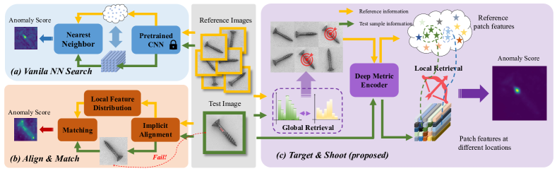
Figure 1: The main scheme of the proposed CPR algorithm. Left-top (a): the vanilla nearest neighbor searching method that searches the neighbors in a brute-force fashion; left-bottom (b): the “align & match” strategy that perform an implicit alignment process before matching; right (c): the proposed “target & shoot” scheme that realize AD within a retrieving cascade.

In this work, by investigating the inherent “matching” character of AD, we propose a more elegant framework to solve the AD problem. We found that a properly selected reference set can significantly benefit the matching process, in terms of both efficiency and accuracy. The main scheme of the proposed framework is shown in Figure 1. As it is illustrated in the left part of the figure, the vanilla nearest-neighbor searching methods retrieve the closest prototype for the test patch in a brute-force way over the whole reference “bank” [28, 29, 30, 31, 32, 33]. In this way, an anomalous patch could be “perfectly” matched with a normal patch, which is totally geometrically irrelevant to the query sample. Consequently, this unconvincing patch matching/retrieval usually implies a failure of AD at the corresponding local region. The “align & match” strategy [34, 35, 36] seems a better alternative as the images are firstly aligned to generate geometrically meaningful matching pairs. However, when the alignment fails on the test image, the geometrical constraint could cause even worse AD results. On the contrary, we perform the retrieval in a “target & shoot” fashion. As we can see in the right part of Figure 1, instead of aligning the test image, we select proper reference “targets” for each test patch. In specific, the qualified target samples should locate at similar image coordinates to the test patch and should be only extracted from the reference images obtained in the global retrieval stage. The local retrieval is conducted in the feature space which is learned using a carefully customized contrastive loss and enjoys high accuracy. In addition, differing from the “align & match” strategy, the cascade scheme is naturally robust to global retrieval errors, and thus the high recall rate of retrieval is ensured.

We term the proposed method “Cascade Patch Retrieval” (CPR) because the retrieval is realized with a two-stage cascade process. For each test patch, our CPR model first selects qualified reference samples in the oracle and then matches the query patch with the selected references. In metaphorical words, the CPR “targets” on the proper references before “shooting”. In the extensive experiments of this work, the proposed “target & shoot” methodology illustrates remarkably high AD accuracy as well as time efficiency. In summary, the contribution of this work is threefold, as listed below.

• Firstly, we cast the AD task as a cascade retrieval problem. Instead of brute force searching over the patch bank or aligning the test image to a “standard” pose, the cascade retrieval strategy naturally possesses a high retrieving recall rate and offers sufficient room for learning better retrieval metrics.

• Secondly, to address the over-fitting problem under the few sample condition for most AD datasets, we propose a novel metric learning framework with a customized contrastive loss and a more conservative learning strategy. The yielded CPR model outperforms existing SOTA algorithms by large margins, in three well-acknowledged AD datasets, namely MVTec AD, MVTec-3D AD and BTAD.

• Finally, in this work, the original CPR algorithm is smartly simplified for higher efficiency. The fastest versions of CPR, i.e., CPR-Faster runs at a speed over $1000$ FPS while still maintaining accuracy superiority over most current SOTA methods.

The rest of this paper is organized as follows: in Section II, the related work of the proposed algorithm is introduced; the details of the CPR algorithm are represented in Section III and we report all the experiment results in Section IV; the Section V summarizes this paper and discusses the future work of CPR.

II Related work

II-A Anomaly Detection via Patch Matching

A simple way to detect and localize anomalies is to find a normal prototype for each test patch and assign high anomaly scores to those with low similarities. As a typical and simple example, the PatchCore algorithm [28] proposes to build a “memory bank” of patch features based on the coreset-subsampling algorithm and the anomaly score is then estimated according to the matching distance between the test patch and its nearest neighbor. Interestingly, merely with this simple matching strategy, PatchCore achieves dramatically high performance on the well-acknowledged MVTech-AD dataset [37]. The success of PatchCore inspired a number of following works: the FAPM algorithm [29] designs patch-wise adaptive coreset sampling to improve the matching speed. [30] improves the matching quality by employing the position and neighborhood information of the test patch. Graphcore [31] proposes a graph representation to adapt PatchCore to the few-shot scenario. Apart from the vanilla brute-force matching, some recently proposed methods [34, 35, 36] try to conduct the patch matching between the test patch and the reference set with similar geometrical properties. In a straightforward way, the test image is firstly aligned to a “standard” pose using rigid [34, 35] or nonrigid [36] geometrical deformations which could be explicitly realized via one or more learnable neural network layers. The aligned deep feature tensor are matched with a reconstructed prototype [36] or a position-conditioned distribution [34, 35] and the anomaly score is estimated according to the deformation magnitude from the prototype [36] or the Mahalanobis distances from each test patch to the corresponding distribution [34, 35].

Despite the well-designed framework, the “align & matching” strategy does not illustrate significant improvement over the non-aligned patch matching methods on the well-acknowledged AD datasets, partially due to the failure cases of image alignment. In this work, we impose the geometrical constraints in another way. Instead of aligning the image, we directly match each test patch with its nearest neighbor, given certain constraints. The constrained searching process is realized in a two-stage retrieval cascade and new SOTA AD performance is obtained.

II-B Deep Learning based Image Retrieval

Image retrieval is a long-standing and fundamental task in computer vision and multimedia. Typically, one needs to find the nearest neighbor(s) of a “query” image over the image “gallery”, which is an image oracle for matching in fact. In this way, the unknown property (e.g. category label or instance identity) of the query image can be determined by the matched nearest neighbors [38]. A great amount of effort has been devoted to realizing better image retrieval algorithms. Most existing image retrieval methods focus on obtaining semantic-aware global features which could be aggregated from the off-the-shelf models [39, 40, 41] or specifically learned models [42, 43, 44]. In particular, to ensure a swift image retrieval process on large-scale datasets, many approaches learn binary codes, instead of conventional real-valued features, to realize the hashing retrieval [45, 46, 47, 48], which is highly efficient in terms of both memory usage and time consumption.

A frequently employed strategy of state-of-the-art retrieval algorithms is the “re-ranking” scheme that consists two phases, i.e., the initial ranking stage and re-ranking stage respectively [49, 50, 44]. In specific, the top-k nearest neighbors are first selected for the query image from a global view in the former stage and the retrieval order is then modified according to the matching state between the local descriptors extracted from the query image and its neighbors. In this work, inspired by the high-level concept of this sophisticated strategy, we smartly transfer the conventional matching operation of anomaly detection into a cascade retrieval problem which is also solved in a coarse to fine manner.

III The proposed method

III-A The overview of the proposed method

The detailed inference scheme of the proposed Cascade Patch Retrieval (CPR) algorithm is shown in Figure 2. According to the illustration, the input of the CPR algorithm includes a test image $\text{I}_{\text{tst}}\in\mathbb{R}^{H_{I}\times W_{I}\times 3}$ and a reference image set $\mathcal{I}_{\text{ref}}\triangleq\{\text{I}^{i}_{\text{ref}}\in\mathbb{R}^{H_{I}\times W_{I}\times 3}\mid i=1,2,\dots,N_{R}\}$. The CNN-based CPR model consists of $4$ subnetworks, namely the DenseNet$201$ [51] backbone, the Global Retrieval Branch (GRB), the Local Retrieval Branch (LRB) and the Foreground Estimation Branch (FEB), respectively. As the raw feature generator, the DenseNet$201$ can be denoted as the following function

$$\Psi_{D}:\text{I}\in\mathbb{R}^{H_{I}\times W_{I}\times 3}\rightarrow\mathfrak{P}\in\mathbb{R}^{H_{P}\times W_{P}\times C_{P}},$$ (1)

where $\mathfrak{P}$ denotes the generated raw feature which will be fed into the succeeding three branches. In a similar manner, the global retrieval branch $\Psi_{G}(\cdot)$, the local retrieval branch $\Psi_{L}(\cdot)$ and the foreground estimation branch $\Psi_{F}(\cdot)$ are defined as follows

$$\begin{split}&\Psi_{G}:\mathfrak{P}\in\mathbb{R}^{H_{P}\times W_{P}\times C_{P}}\rightarrow\mathfrak{G}\in\mathbb{R}^{S\times S\times N_{C}}\\ &\Psi_{L}:\mathfrak{P}\in\mathbb{R}^{H_{P}\times W_{P}\times C_{P}}\rightarrow\mathfrak{L}\in\mathbb{R}^{H_{L}\times W_{L}\times C_{L}}\\ &\Psi_{F}:\mathfrak{P}\in\mathbb{R}^{H_{P}\times W_{P}\times C_{P}}\rightarrow\text{F}\in\mathbb{R}^{H_{F}\times W_{F}}\end{split}$$ (2)

note that the outputs of $\Psi_{G}(\cdot)$ is a collection of $S^{2}$ histograms with $N_{C}$ bins, $\Psi_{L}(\cdot)$ generates a $3$-D tensor while the output of $\Psi_{F}(\cdot)$ is a $2$-D confidence map F.

The first stage of the cascade retrieval is conducted based on the “global feature” $\mathfrak{G}$ and the top-$k$ nearest neighbors of the test image $\text{I}_{\text{tst}}$ is stored into the image set $\mathcal{N}_{\text{ref}}$.

The second stage of the cascade retrieval is performed based on the local feature $\mathfrak{L}\in\mathbb{R}^{H_{P}\times W_{P}\times C_{P}}$ which can be viewed as a collection of $H_{P}\cdot W_{P}$ vector features with each element corresponding to an image patch. The primitive anomaly score of each test patch is estimated according to the patch feature distance between itself and its nearest neighbor retrieved from $\mathcal{N}_{\text{ref}}$ and at similar image locations.

Finally, under the assumption that the anomalies only take place in the foreground part, the primitive anomaly scores are corrected via using the foreground confidence map $\text{F}\in\mathbb{R}^{H_{F}\times W_{F}}$ predicted by the foreground estimation branch $\Psi_{F}(\cdot)$.

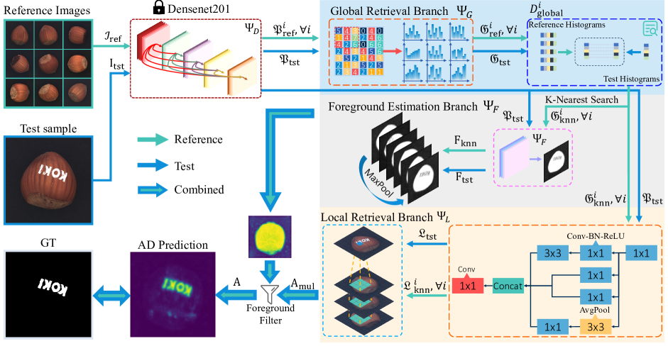
Figure 2: CPR train procedure for detecting and localizing anomalies on images. The whole process could be divided into $4$ sectors, namely the DenseNet$201$ backbone, the global retrieval branch, the local retrieval branch and the foreground estimation branch, respectively.

III-B The global retrieval branch

The Global Retrieval Branch (GRB) is actually a statistical feature generator. Given $N_{R}$ reference (anomaly-free) images $\{\text{I}^{i}_{\text{ref}}\in\mathbb{R}^{H_{I}\times W_{I}\times 3}\mid i=1,2,\dots,N_{R}\}$, and the corresponding DenseNet feature tensors $\{\mathfrak{P}^{i}_{\text{ref}}=\Psi_{D}(\text{I}^{i}_{\text{ref}})\mid i=1,2,\dots,N_{R}\}$, we firstly flatten each tensor to build the “raw patch feature” set as

$$\mathfrak{P}^{i}_{\text{ref}}\xrightarrow{\texttt{flatten}}\{\vec{\mathbf{p}}^{i,j}_{\text{ref}}\in\mathbb{R}^{C_{P}}\mid j=1,2,\dots,H_{P}W_{P}\}$$ (3)

Then suppose all the raw patch features belonging to different reference images are collected together into the feature set $\mathcal{P}_{\text{ref}}\triangleq\{\vec{\mathbf{p}}^{u}_{\text{ref}}\in\mathbb{R}^{C_{P}}\mid u=1,2,\dots,N_{R}H_{P}W_{P}\}$, a $K$-means clustering method is performed on $\mathcal{P}_{\text{ref}}$ to obtain $N_{C}$ clustering centers $\mathcal{C}_{\text{ref}}\triangleq\{\vec{\mathbf{c}}^{v}_{\text{ref}}\in\mathbb{R}^{C_{P}}\mid v=1,2,\dots,N_{C}\}$.

The block-wise statistics of the test image $\text{I}_{\text{tst}}$ can be obtained based on the raw feature tensor $\mathfrak{P}_{\text{tst}}$ and the cluster center set $\mathcal{C}_{\text{ref}}$. In specific, the tensor $\mathfrak{P}_{\text{tst}}$ is evenly divided into $S\times S$ sub-tensors as

$$\hat{\mathfrak{P}}^{u,v}_{\text{tst}}\in\mathbb{R}^{\frac{H_{P}}{S}\times\frac{W_{P}}{S}\times C_{P}},u,v=1,2,\dots,S.$$

For each sub-tensor, we extract its statistics in the “Bag of Words” (BoW) style as

$$\begin{split}\hat{\mathfrak{P}}^{u,v}_{\text{tst}}&\xrightarrow{\texttt{flatten}}\mathcal{P}_{\text{tst}}\triangleq\{\vec{\mathbf{p}}^{i}_{\text{tst}}\mid i=1,\dots,\frac{H_{P}W_{P}}{S^{2}}\}\\ &\xrightarrow{\texttt{BoW}}\vec{\mathbf{h}}_{u,v}\in\mathbb{R}^{N_{C}},\forall u,v\end{split}$$ (4)

where $\vec{\mathbf{h}}_{u,v}$ denotes a BoW histogram of $\hat{\mathfrak{P}}^{u,v}_{\text{tst}}$ with respect to the codebook $\mathcal{C}_{\text{ref}}$ and this histogram is normalized so that $\|\vec{\mathbf{h}}_{u,v}\|_{l_{1}}=1,\forall u,v$. The histograms of a reference image $\text{I}^{i}_{\text{ref}}$ can also be obtained in a similar manner as Equation 4 and let us denote them as $\vec{\mathbf{h}}^{\text{ref}}_{u,v,i}$. Let $D^{u,v,i}_{\text{KL}}\triangleq\text{KL}(\vec{\mathbf{h}}^{\text{ref}}_{u,v,i},\vec{\mathbf{h}}_{u,v})$ denote the Kullback-Leibler (KL) divergence between two block histograms with the same block ID, one can get the following sorted (in increasing order) block divergences

$$\{D^{i}_{1}\leqslant D^{i}_{2}\leqslant D^{i}_{3}\dots\leqslant D^{i}_{S^{2}}\}.$$

Then the global features distance between $\text{I}_{\text{tst}}$ and $\text{I}^{i}_{\text{ref}}$ is estimated as

$$D^{i}_{\text{global}}\triangleq\frac{1}{S^{2}-\tau}\sum_{j=1}^{S^{2}-\tau}D^{i}_{j},~{}\forall i=1,2,\dots,N_{R},$$ (5)

where $\tau$ is a small number for ignoring large block-wise KL divergences so that the overall distance estimation is robust to partial image contamination.

Based on the global feature distance, the top-$K$ neighbor reference images are retrieved for $\text{I}_{\text{tst}}$ and stored into the image set $\mathcal{N}_{\text{ref}}\triangleq\{\text{I}^{1}_{\text{knn}},\text{I}^{2}_{\text{knn}},\dots,\text{I}^{K}_{\text{knn}}\}$ which are employed as the reference images in the following patch retrieval process.

In practice, this searching process over the reference images usually lead to a set of “pseudo-aligned” nearest neighbors (see Section IV-E for details). Thus our global retrieval branch offers an alternative to the image alignment approaches [34, 35, 36], while with higher simplicity and accuracy.

III-C The local retrieval branch

The Local Retrieval Branch (LRB) plays the most important role in the CPR algorithm.

III-C1 The structure of LRB

As to the branch structure, inspired by the pioneering work [52], we modify the well-known inception block to build our LRB. As it is shown in Figure 2, the input feature (i.e., the raw feature tensor $\mathfrak{P}$ of Equation 1) are processed by the block via four main paths, with different combinations of the “Conv-BN-ReLU” blocks and the average pooling layers. The output tensors of these four paths are firstly concatenated together and then further processed by a $1\times 1$ convolutional layer. According to Equation 2, the final output tensor of the test image $\text{I}_{\text{tst}}$ is given by

$$\mathfrak{L}_{\text{tst}}=\Psi_{L}(\Psi_{D}(\text{I}_{\text{tst}}))\in\mathbb{R}^{H_{L}\times W_{L}\times C_{L}}.$$ (6)

III-C2 The inference process of LRB

Let us flatten the tensor $\mathfrak{L}_{\text{tst}}$ into a set of feature vectors with the associated row-column coordinates as

$$\mathfrak{L}_{\text{tst}}\xrightarrow{\texttt{flatten}}\mathcal{L}_{\text{tst}}\triangleq\{\vec{\mathbf{l}}^{r,c}_{\text{tst}}\in\mathbb{R}^{C_{L}}\mid\forall r,c\},$$ (7)

where $r=1,2,\dots,H_{L}$, $c=1,2,\dots,W_{L}$.

Given the nearest neighbor set $\mathcal{N}_{\text{ref}}$ obtained by GRB, one can calculate the corresponding local feature tensors as $\{\mathfrak{L}^{j}_{\text{knn}}=\Psi_{L}(\Psi_{D}(\text{I}^{j}_{\text{knn}}))\in\mathbb{R}^{H_{L}\times W_{L}\times C_{L}}\mid j=1,2,\dots,K\}$. In a similar way to Equation 7, the feature vectors of $\mathcal{N}_{\text{ref}}$ writes

$$\{\mathfrak{L}^{j}_{\text{knn}}\mid\forall j\}\xrightarrow{\texttt{flatten}}\mathcal{L}_{\text{knn}}\triangleq\{\vec{\mathbf{l}}^{r,c,j}_{\text{knn}}\in\mathbb{R}^{C_{L}}\mid\forall r,c,j\},$$ (8)

The local patch retrieval is then conducted between each feature vector in $\mathcal{L}_{\text{tst}}$ and the patch reference set $\mathcal{L}_{\text{knn}}$. In particular, given a test patch feature $\vec{\mathbf{l}}^{r,c}_{\text{tst}}$, its nearest neighbor is retrieved as

$$\vec{\mathbf{l}}^{\ast}_{r,c}=\operatorname*{argmin}_{\begin{subarray}{c}\forall|\bar{r}-r|<\delta\\ \forall|\bar{c}-c|<\delta\\ \forall j=1,\dots,K\end{subarray}}\left[1-\Phi_{\text{cos}}(\vec{\mathbf{l}}^{r,c}_{\text{tst}},\vec{\mathbf{l}}^{\bar{r},\bar{c},j}_{\text{knn}})\right],$$ (9)

where $\Phi_{\text{cos}}(\cdot)$ stands for the function of cosine similarity between two vectors. Accordingly, the minimal distance is defined as:

$$\text{A}_{\text{ori}}[r,c]=d^{\ast}_{r,c}\triangleq 1-\Phi_{\text{cos}}(\vec{\mathbf{l}}^{r,c}_{\text{tst}},\vec{\mathbf{l}}^{\ast}_{r,c}),$$ (10)

where $\text{A}_{\text{ori}}\in\mathbb{R}^{H_{L}\times W_{L}}$ denotes the map of anomaly score predicted by the LRB.

III-C3 The training strategy of LRB

To achieve a good metric function $\Psi_{\text{L}}$ for patch retrieval, we learn the parameters of LRB using a sophisticated training scheme and a modified contrastive loss [53].

In particular, firstly, a query image $\text{I}_{\text{que}}$ and a reference image $\text{I}_{\text{ref}}$ randomly selected from the $K$-NN set $\mathcal{N}_{\text{ref}}$ are employed as the input of the metric learning process. Following the data augmentation strategy of [18], pseudo anomalies are randomly merged with $\text{I}_{\text{que}}$ to generate the synthetically defective image $\tilde{\text{I}}_{\text{que}}$. Secondly, $\tilde{\text{I}}_{\text{que}}$ and $\text{I}_{\text{ref}}$ are processed by Equation 6 to obtain the feature tensors $\mathfrak{L}_{\text{que}}$ and $\mathfrak{L}_{\text{ref}}$ which are further flattened to the vector feature sets $\mathcal{L}_{\text{que}}\triangleq\{\vec{\mathbf{l}}^{r,c}_{\text{que}}\in\mathbb{R}^{C_{L}}\mid\forall r,c\}$ and $\mathcal{L}_{\text{ref}}\triangleq\{\vec{\mathbf{l}}^{r,c}_{\text{ref}}\in\mathbb{R}^{C_{L}}\mid\forall r,c\}$ respectively.

Thirdly, the training samples of the metric learning, i.e., the feature pairs are sampled using Algorithm 1. Note that three kinds of feature pairs are sampled, namely the positive pairs, the remote pairs and the anomalous pairs. The former one is positive ($y_{i}=1$) and the latter two kinds are both negative ($y=0$) but differ in the reason for being negative.

Input: Query feature set $\mathcal{L}_{\text{que}}$; reference feature set $\mathcal{L}_{\text{ref}}$; binary mask $\text{M}_{\text{que}}\in\mathbb{B}^{H_{L}\times W_{L}}$ of the synthetic anomaly of $\tilde{\text{I}}_{\text{que}}$; number of samples $\Gamma$; distance threshold $\theta$; vector normalization function $\Phi(\cdot)$.

Output: The set of query-reference feature pairs $\Xi=\{\xi_{i}=[\vec{\boldsymbol{\eta}}^{i}_{\text{que}},\vec{\boldsymbol{\eta}}^{i}_{\text{ref}}]\mid i=1,\dots,\Gamma\}$; Binary labels $\vec{\mathbf{y}}\in\mathbb{B}^{\Gamma}$.

1 Algorithm:

2 $\Xi\leftarrow\{\}$, $\vec{\mathbf{y}}=\mathbf{0},i=1$

3 while $i\leqslant\Gamma$ do

       /* positive pairs sampling */

4       $[r_{q},~{}c_{q}]=\texttt{RandSelect}([\![\text{M}_{\text{que}}==0]\!])$

5       $[r_{r},~{}c_{r}]=[r_{q},~{}c_{q}]$

6       $\Xi\leftarrow\xi_{i}=[\Phi(\vec{\mathbf{l}}^{r_{q},c_{q}}_{\text{que}}),\Phi(\vec{\mathbf{l}}^{r_{r},c_{r}}_{\text{ref}})]$, $\vec{\mathbf{y}}[i]=1$

7      

      /* remote pairs sampling */

8       $[r_{q},c_{q}]=\texttt{RandSelect}([\![\|r_{r}-r_{q},c_{r}-c_{q}\|_{l_{2}}>\theta]\!])$

9       $\Xi\leftarrow\xi_{i}=[\Phi(\vec{\mathbf{l}}^{r_{q},c_{q}}_{\text{que}}),\Phi(\vec{\mathbf{l}}^{r_{r},c_{r}}_{\text{ref}})]$, $\vec{\mathbf{y}}[i+1]=0$

10      

      /* anomalous pairs sampling */

11       $[r_{q},~{}c_{q}]=\texttt{RandSelect}([\![\text{M}_{\text{que}}==1]\!])$

12       $[r_{r},~{}c_{r}]=[r_{q},~{}c_{q}]$

13       $\Xi\leftarrow\xi_{i}=[\Phi(\vec{\mathbf{l}}^{r_{q},c_{q}}_{\text{que}}),\Phi(\vec{\mathbf{l}}^{r_{r},c_{r}}_{\text{ref}})]$, $\vec{\mathbf{y}}[i+2]=0$

14      

15      $i=i+3$

16      

17 end while

Algorithm 1 Feature-pair sampling strategy of CPR

Fourthly, in Algorithm 1, a remote pair is considered as negative only because of the coordinate distance between the two involved features. In this way, unnecessary ambiguities could be brought into the training process due to the existence of the “remote but similar” feature pairs. In this work, we propose to reduce the training sample weights of those ambiguous pairs. Concretely, given the row-column coordinates of the two involved features in a pair $\xi_{i}$ writes $[r_{i},c_{i},\hat{r}_{i},\hat{c}_{i}]$, $\omega_{i}$ and the raw feature tensors of query and reference images are $\mathfrak{P}_{\text{que}}=\Psi_{D}(\tilde{\text{I}}_{\text{que}})$ and $\mathfrak{P}_{\text{ref}}=\Psi_{D}(\text{I}_{\text{ref}})$ . The weight of $\xi_{i}$ is denoted as $\omega_{i}$ which is calculated as

$$\omega_{i}=\begin{cases}\|\vec{\mathbf{p}}^{r,c}_{\text{que}}-\vec{\mathbf{p}}^{\hat{r},\hat{c}}_{\text{ref}}\|_{l_{2}}/\delta&\text{if }\xi_{i}~{}\text{is a remote pair}\\ 1&\text{otherwise}\end{cases}$$ (11)

where $\vec{\mathbf{p}}^{r,c}_{\text{que}}$ and $\vec{\mathbf{p}}^{\hat{r},\hat{c}}_{\text{ref}}$ are the sliced feature vectors from $\mathfrak{P}_{\text{que}}$ and $\mathfrak{P}_{\text{ref}}$, according to the coordinates $[r_{i},c_{i},\hat{r}_{i},\hat{c}_{i}]$, $\|\cdot\|_{l_{2}}$ stands for the $l_{2}$ norm function and $\delta$ is the pre-estimated average raw feature distance between randomly selected reference and query images.

Finally, the modified contrastive loss is defined as

$$\begin{split}\mathsf{L}_{\text{contrast}}=&\frac{1}{\Gamma}\sum^{\Gamma}_{i=1}\omega_{i}\cdot[y_{i}\cdot\text{max}(0,m^{+}-{\vec{\boldsymbol{\eta}}^{i~{}\text{T}}_{\text{que}}}\vec{\boldsymbol{\eta}}^{i}_{\text{ref}})+\\ &(1-y_{i})\cdot\text{max}(0,\vec{\boldsymbol{\eta}}^{i~{}\text{T}}_{\text{que}}\vec{\boldsymbol{\eta}}^{i}_{\text{ref}}-m^{-})]^{p},\end{split}$$ (12)

where the inner product between $\vec{\boldsymbol{\eta}}^{i}_{\text{que}}$ and $\vec{\boldsymbol{\eta}}^{i}_{\text{ref}}$ reflects the pair similarity, $m^{+}$ and $m^{-}$ are the hyper-parameters of “similarity threshold” for positive pairs and negative pairs, $p$ is a constant set larger than $1$ to emphasis the hard pair samples in training.

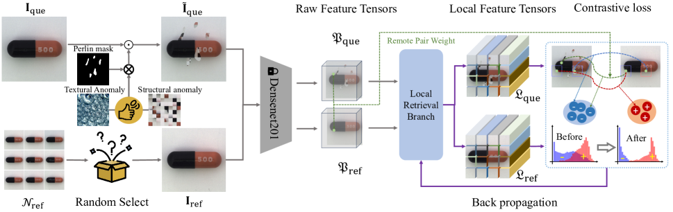
Figure 3: CPR inference procedure for detecting and localizing anomalies on images. Note that the remote feature pairs (green) and the anomalous feature pairs (blue) are labeled as negative while the positive feature pairs (red) are extracted from the identical and defect-free location on two feature tensors.

III-D The foreground estimation branch

In many real-life scenarios, the inspected object (e.g. a screw or a hazelnut [37]) is photographed with a large surrounding background region and without explicit annotations. Recalling that the concerned anomalies are all located on the object part, removing the “false alarms” on the background region can therefore effectively increase the AD accuracy. Consequently, in some recently proposed works [18, 54, 55, 56], foreground/background information is well exploited for anomaly detection.

In this paper, we employ a Foreground Estimating Branch (FEB) to classify the pixels as foreground or background. The workflow of FEB is depicted in Figure 4. As it is shown in the figure, firstly, each training image $\text{I}^{i}_{\text{ref}}$ is processed by DenseNet$201$ backbone as Equation 1 to generate the raw feature tensor $\mathfrak{P}^{i}_{\text{ref}}\in\mathbb{R}^{H_{P}\times W_{P}\times C_{P}}$. Secondly, all the vector feature $\vec{\mathbf{p}}^{i,j}_{\text{ref}}\in\mathbb{R}^{C_{P}},\forall j$ of this tensor are coded with the codebook $\mathcal{C}_{\text{ref}}$ defined in Section III-B and then the codes are recombined into a code map $\text{C}^{i}_{\text{ref}}\in\mathbb{R}^{H_{P}\times W_{P}}$ (shown as numbers on the right column of Figure 4), which is mainly used to select training samples for FEB.

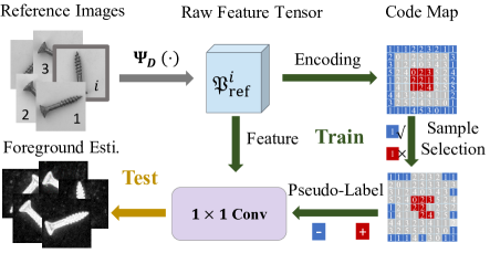
Figure 4: The foreground estimation strategy of the proposed CPR method. The deep features obtained by DenseNet$201$ and the pseudo-labels are used to learn a $1\times 1$ convolutional layer.

In this work, some of the vector features $\vec{\mathbf{p}}^{i,j}_{\text{ref}}\in\mathbb{R}^{C_{P}},\forall j$ of this tensor are selected as training features of the classifier. As there is no explicit foreground/background label in most AD datasets [37, 57], we propose to generate the pseudo-labels for the selected deep features. In general, the surrounding area (shown in blue in the top-right block of Figure 4) are treated as negative (background) regions and the center area (shown in red in the two blocks) are the positive (foreground) region. However, to further remove the potential class ambiguity, only the surrounding features with the majority code (cluster-$1$ in the example of Figure 4) are selected as negative samples and the center samples with this majority code are abandoned. The training samples of the FEB is selected over all the reference images and a $1\times 1$ convolutional layer is employed to classify the vector features $\vec{\mathbf{p}}^{i,j}_{\text{ref}},\forall j$ into the two categories, as shown in the bottom-left corner of Figure 4.

In practice, suppose that the foreground prediction map of the test image $\text{I}_{\text{tst}}$ is denoted as $\text{F}_{\text{tst}}\in\mathbb{R}^{H_{F}\times W_{F}}$ and those maps of $\text{I}_{\text{tst}}$’s $K$ nearest neighbors are collected in the set $\mathcal{F}\triangleq\{\text{F}^{i}_{\text{ref}}\in\mathbb{R}^{H_{F}\times W_{F}}\mid i=1,2,\dots,K\}$, each element of the final foreground estimation map $\text{F}^{\ast}\in\mathbb{R}^{H_{F}\times W_{F}}$ is given by

$$\text{F}^{\ast}[r,c]=\max\left(\text{F}_{\text{tst}}[r,c],~{}\max_{i=1,\dots,K}\text{F}^{i}_{\text{ref}}[r,c]\right),$$ (13)

where $r=1,\dots H_{F}$ and $c=1,\dots,W_{F}$. The final anomaly prediction map $\text{A}^{\ast}\in\mathbb{R}^{H_{F}\times W_{F}}$ is then obtained as

$$\text{A}^{\ast}=\texttt{UpInterp}(\text{A}_{\text{ori}})\odot\text{F}^{\ast},$$ (14)

where $\odot$ denotes the element-wise multiplication and function $\texttt{UpInterp}(\cdot)$ stands for the up-sampling operation as $\text{A}_{\text{ori}}\in\mathbb{R}^{H_{L}\times W_{L}}$ and usually $H_{F}\geqslant H_{L}~{}\&~{}W_{F}\geqslant W_{L}$. Note that the proposed FEB is not compatible to all the AD datasets, e.g. the texture sub-categories of MVTec AD [58]. In these scenarios, we just disable the FEB for the whole learning-inference process.

III-E The end-to-end inference process of CPR

The end-to-end inference process of the proposed method is shown in Algorithm 2. Note that in practice the proposed method is designed in a multi-scale style. In particular, two raw feature tensors $\mathfrak{P}^{j},j\in\{1,2\}$ are extracted from different layers of DenseNet$201$. The GRB and the FEB are only conducted on $\mathfrak{P}^{1}$ with higher resolution while the local patch retrieval is performed on both of the two tensors. The yielded two anomaly score maps $\text{A}^{1}_{\text{ori}}$ and $\text{A}^{2}_{\text{ori}}$ are firstly aggregated and then fused with the foreground estimation $\text{F}^{\ast}$ to generate the final score map $\text{A}^{\ast}$. In addition, the image-level anomaly score $\alpha^{\ast}$ is estimated using the similar method as [54, 22].

Input: Two pre-trained feature extractors of DenseNet$201$: $\Psi_{D}^{l}(\cdot),l\in\{1,2\}$; GRB $\Psi_{G}(\cdot)$, global feature oracle $\mathcal{G}_{\text{ref}}$; LRB $\Psi_{L}(\cdot)$; local feature oracles with multi-scale $\mathcal{L}^{l}_{\text{ref}},l\in\{1,2\}$; FEB $\Psi_{F}(\cdot)$; foreground estimation map set $\mathcal{F}_{\text{ref}}$; number of nearest neighbors $K$; test image $\text{I}_{\text{tst}}$.

Output: Anomaly score map $\text{A}_{\text{tst}}$ and anomaly score $\alpha_{\text{tst}}$ for $\text{I}_{\text{tst}}$.

1 Algorithm:

/* Feature extraction */

2 for $l\in\{1,2\}$ do

3       $\mathfrak{P}_{\text{tst}}^{l}=\Psi_{D}^{l}(\text{I}_{\text{tst}})$

4 end for

5$\mathfrak{G}_{\text{tst}},\text{F}_{\text{tst}}=\Psi_{G}(\mathfrak{P}_{\text{tst}}^{1}),\Psi_{F}(\mathfrak{P}_{\text{tst}}^{1})$

/* Find the $K$-NNs of $\mathfrak{G}_{\text{tst}}$ in $\mathcal{G}_{\text{ref}}$ */

6 $\boldsymbol{\beta}_{\text{knn}}=\texttt{KNN-Idx}(\mathfrak{G}_{\text{tst}},\mathcal{G}_{\text{ref}})\in\mathbb{N}^{K}$

7

8$\mathcal{F}_{\text{knn}}=\mathcal{F}_{\text{ref}}[\boldsymbol{\beta}_{\text{knn}}]$

9

10$\text{F}^{*}=\texttt{MaxPool}(\mathcal{F}_{\text{knn}}\cup\text{F}_{\text{tst}})$

/* multiscale local retrieval */

11 $\text{A}_{\text{mul}}=\text{0}\in\mathbb{R}^{H_{L}\times W_{L}}$

12

13for $l\in\{1,2\}$ do

14      

15      $\mathfrak{L}^{l}_{\text{tst}}=\Psi_{L}(\mathfrak{P}^{l}_{\text{tst}})$

16      

17      $\mathfrak{L}^{l}_{\text{tst}}\xrightarrow{\texttt{flatten}}\mathcal{L}_{\text{tst}}=\{\vec{\mathbf{l}}^{r,c}_{\text{tst}}\in\mathbb{R}^{C_{L}}\mid\forall r,c\}$

18      

19      $\mathcal{L}^{l}_{\text{ref}}[\boldsymbol{\beta}_{\text{knn}}]\xrightarrow{\texttt{flatten}}\mathcal{L}_{\text{knn}}=\{\vec{\mathbf{l}}^{r,c,j}_{\text{knn}}\in\mathbb{R}^{C_{L}}\mid\forall r,c,j\}$

20      

21      for $r\in\{1,\dots,H_{L}\}$ and $c\in\{1,\dots,W_{L}\}$ do

22             $\vec{\mathbf{l}}^{\ast}_{r,c}=\texttt{LocalNN}(\vec{\mathbf{l}}^{r,c}_{\text{tst}},\mathcal{L}_{\text{knn}})$ as 9 $\text{A}_{\text{ori}}^{l}[r,c]=1-\Psi_{\text{cos}}(\vec{\mathbf{l}}^{r,c}_{\text{tst}},\vec{\mathbf{l}}^{\ast}_{r,c})$

23            

24       end for

25      $\text{A}_{\text{mul}}=\text{A}_{\text{mul}}+\texttt{UpInterp}(\text{A}_{\text{ori}}^{l})$

26      

27 end for

/* foreground filter */

28 $\text{A}^{\ast}=\text{A}_{\text{mul}}\odot\text{F}^{\ast}$

/* image-level anomaly score */

$\alpha^{\ast}=\sum_{i=1}^{T}\texttt{sort}^{\Downarrow}(\texttt{flatten}(\text{A}^{\ast}))$

Algorithm 2 Inference pseudo-code of CPR

III-F Implementation details

The input images of our CPR model are consistently resized to $320\times 320$, in both training and test procedures. We adopt the “denseblock-$1$” and “denseblock-$2$” of the DenseNet$201$ model [51] pre-trained on ImageNet [59] to obtain the raw feature tensors with the sizes $256\times 80\times 80$ and $512\times 40\times 40$ respectively and freeze these blocks during training. In particular, GRB and FEB only performed based on denseblock-$1$ and LRB uses both denseblock-$1$ and denseblock-$2$ in a multi-scale manner.

The dimension of the feature space for local retrieval is $384$, following the setting in [28]. In the inference stage, the number of $K$ nearest neighbors is $10$, the size of the sub-tensors $S$ is set to 5, the number of clusters $N_{c}$ is $12$, the parameter for robust KL divergences $\tau$ is set to $5$, the parameter $T$ for calculating image-level anomaly score is $512$ and the local retrieval region size for denseblock-$1$ and denseblock-$2$ are $3$ and $1$ respectively.

As to the training setup, we use the AdamW optimizer [60] to update the model parameters with a default learning rate $1\times 10^{-3}$ and default weight decay rate $1\times 10^{-2}$. The training is conducted for $40000$ iterations with the batch size $32$ for each sub-category and we empirically select A FIXED iteration number for ALL THE SUB-CATEGORIES of one dataset . In this paper, the data augmentation only contains the salt-and-pepper noise and the brightness changes.

We adopt off-the-shelf defect generation/augmentation approaches in this paper. For the anomaly-free training sets, synthetic anomalies are randomly generated and added onto the normal samples, mainly following the pseudo-defect generation method proposed in [18]. For the supervised scenarios, we employ a similar strategy as the PRN algorithm [54] to “extend” the anomalous patterns for achieving better performance based on limited samples.

IV Experiments

In this section, a series of experiments are conducted to verify the proposed method, comparing with other state-of-the-art methods. Three well-acknowledged benchmark datasets, namely the MVTec AD [37], MVTec-3D AD [57] and BTAD [61] are involved in the experiments. The anomaly detection and localization performances are evaluated using four popular AD metrics, i.e., Image-AUC, Pixel-AUC, Per-Region Overlap (PRO), and Average Precision (AP), under both the supervised and unsupervised scenarios.

IV-A Experimental settings

IV-A1 Three involved datasets

• MVTec AD [58] contains $5354$ images belonging to $15$ sub-datasets which can be further split into $10$ object sub-categories and $5$ texture sub-categories. Each sub-category involves a nominal-only training set and a test set with various types of anomalies.

• MVTec-3D AD [57] is a 3D anomaly detection dataset comprising over $4000$ RGB images and the corresponding high-resolution 3D point cloud data. Similar to MVTec AD, each of the $10$ sub-categories of MVTec-3D AD are divided into a defect-free training set and a test set containing various kinds of defects. Though MVTec-3D AD provides accurate point cloud information, only RGB images are utilized for predicting anomalies in this work.

• BTAD [61] comprises $2540$ images from three categories of real-world industrial products with different body and surface defects. It is usually considered as a complementary dataset to the MVTec AD when evaluating an AD algorithm.

IV-A2 Four evaluation metrics

• Image-AUC: this image-level AD performance is measured by calculating the area under the “Receiver Operating Characteristic” curve (AUROC) of the predicted image-level anomaly scores with increasing thresholds.

• Pixel-AUC: this pixel-level AD performance is similar to the image-AUC except that the unit to be classified is pixel rather than image.

• PRO: the “Per-Region Overlap” metric is a pixel-level metric that evaluates the AD performance on connected anomaly regions. It is more robust to the dataset with significantly different sizes of anomaly regions [62].

• AP: the average precision (AP) is the most popular metric for semantic segmentation tasks. It treats each pixel independently when measuring the segmentation performance [63].

IV-A3 Two supervision scenarios

• The unsupervised scenario. This is the conventional supervision condition in the literature of AD [58, 57, 61]. In this scenario, all the training images are anomaly free while various anomalies exist in the test set. To achieve a better AD model, we train our CPR algorithm by using synthetic defects as it is introduced in Section III-E.

• The supervised scenario. To mimic the real-life situation where a limited number of defective samples are available, some researchers [64, 54] propose to randomly select some anomalous test samples and add them to the original training set. The yielded AD models usually perform better on the remaining test images. In this work, we employ the “Extended Anomalies” strategy [54] to further exploit the information of the genuine defects.

IV-A4 Hardware setting

We conduct all the mentioned experiments in this paper using a machine equipped with an Intel i$5$-$13600$KF CPU, 32G DDR4 RAM and an NVIDIA RTX $4090$ GPU.

IV-B Quantitative Results

IV-B1 Results in unsupervised setting

We firstly evaluate the proposed method and the $8$ comparing SOTA methods (PatchCore [28], DRAEM [17], RD [20], SSPCAB [65], DeSTSeg [22], PyramidFlow [15], CDO [66] and SemiREST [67]) on the MVTec AD dataset [58] and within the unsupervised condition. Table I shows the AP, PRO and Pixel-AUC results of the involved methods. According to the table, our CPR algorithm outperforms other competitors by large margins. The most recently proposed SemiREST algorithm [67] performs slightly better than our method on the texture sub-categories while CPR beats it on the object sub-categories with significant superiority (e.g., the nearly $3\%$ gain on AP). In general, the proposed CPR method ranks first for the AP and PRO metrics and ranks second for the Pixel-AUC metric. We report the Image-AUC scores of the comparing methods in Table II, from which one can see a new Image-AUC record of $99.8\%$ is achieved by the proposed method. This performance is achieved by selecting the best training iteration number independently for each sub-category. Although contradicting the principle of model selection described in Section III-F, this model selection trick is common in the literature of anomaly detection [14, 68, 66]. When strictly following the model selection principle in Section III-F, the Image-AUC drops marginally to $99.7\%$ which is also higher than the existing SOTA performances.

TABLE I: The AP, PRO and Pixel-AUROC scores on MVTec AD in the unsupervised settings.

Category	PatchCore [28] (CVPR2022)	DRAEM [17] (ICCV2021)	RD [20] (CVPR2022)	SSPCAB [65] (CVPR2022)	DeSTSeg [22] (CVPR2023)	PyramidFlow [15] (CVPR2023)	CDO [66] (TII2023)	SemiREST [67] (arXiv2023)	Ours
Carpet	$64.1$/$95.1$/$\mathbf{99.1}$	$53.5$/$92.9$/$95.5$	$56.5$/$95.4$/$98.9$	$48.6$/$86.4$/$92.6$	$72.8$/$93.6$/$96.1$	$\sim$/$97.2$/$97.4$	$53.4$/$96.8$/$\mathbf{99.1}$	$\mathbf{84.2}$/$\mathbf{98.7}$/$\mathbf{99.6}$	$\mathbf{81.2}$/$\mathbf{97.6}$/$98.9$
Grid	$30.9$/$93.6$/$98.8$	$\mathbf{65.7}$/$\mathbf{98.3}$/$\mathbf{99.7}$	$15.8$/$94.2$/$98.3$	$57.9$/$\mathbf{98.0}$/$\mathbf{99.5}$	$61.5$/$96.4$/$99.1$	$\sim$/$94.3$/$95.7$	$45.3$/$96.1$/$98.4$	$\mathbf{65.5}$/$97.9$/$\mathbf{99.5}$	$64.0$/$97.6$/$\mathbf{99.5}$
Leather	$45.9$/$97.2$/$99.3$	$75.3$/$97.4$/$98.6$	$47.6$/$98.2$/$99.4$	$60.7$/$94.0$/$96.3$	$75.6$/$99.0$/$\mathbf{99.7}$	$\sim$/$99.2$/$98.7$	$43.6$/$98.3$/$99.2$	$\mathbf{79.3}$/$\mathbf{99.4}$/$\mathbf{99.8}$	$\mathbf{78.5}$/$\mathbf{99.6}$/$\mathbf{99.8}$
Tile	$54.9$/$80.2$/$95.7$	$92.3$/$\mathbf{98.2}$/$99.2$	$54.1$/$85.6$/$95.7$	$\mathbf{96.1}$/$98.1$/$\mathbf{99.4}$	$90.0$/$95.5$/$98.0$	$\sim$/$97.2$/$97.1$	$61.8$/$90.5$/$97.2$	$\mathbf{96.4}$/$\mathbf{98.5}$/$\mathbf{99.7}$	$94.1$/$98.1$/$99.2$
Wood	$50.0$/$88.3$/$95.0$	$77.7$/$90.3$/$96.4$	$48.3$/$91.4$/$95.8$	$78.9$/$92.8$/$96.5$	$\mathbf{81.9}$/$96.1$/$\mathbf{97.7}$	$\sim$/$\mathbf{97.9}$/$97.0$	$46.3$/$92.9$/$95.8$	$79.4$/$96.5$/$\mathbf{97.7}$	$\mathbf{80.8}$/$\mathbf{97.7}$/$\mathbf{97.4}$
Average	$49.2$/$90.9$/$97.6$	$72.9$/$95.4$/$97.9$	$44.5$/$93.0$/$97.6$	$68.4$/$93.9$/$96.9$	$76.4$/$96.1$/$98.1$	$\sim$/$\mathbf{97.2}$/$97.2$	$50.1$/$96.5$/$98.0$	$\mathbf{81.0}$/$\mathbf{98.2}$/$\mathbf{99.3}$	$\mathbf{79.7}$/$\mathbf{98.2}$/$\mathbf{99.0}$
Bottle	$77.7$/$94.7$/$98.5$	$86.5$/$96.8$/$99.1$	$78.0$/$96.3$/$98.8$	$89.4$/$96.3$/$99.2$	$90.3$/$96.6$/$99.2$	$\sim$/$95.5$/$97.8$	$84.1$/$97.2$/$99.3$	$\mathbf{94.1}$/$\mathbf{98.6}$/$\mathbf{99.6}$	$\mathbf{92.6}$/$\mathbf{98.1}$/$\mathbf{99.4}$
Cable	$66.3$/$93.2$/$98.4$	$52.4$/$81.0$/$94.7$	$52.6$/$94.1$/$97.2$	$52.0$/$80.4$/$95.1$	$60.4$/$86.4$/$97.3$	$\sim$/$90.3$/$91.8$	$61.0$/$94.2$/$97.6$	$\mathbf{81.1}$/$\mathbf{95.3}$/$\mathbf{99.1}$	$\mathbf{84.4}$/$\mathbf{95.2}$/$\mathbf{99.3}$
Capsule	$44.7$/$94.8$/$99.0$	$49.4$/$82.7$/$94.3$	$47.2$/$95.5$/$98.7$	$46.4$/$92.5$/$90.2$	$56.3$/$94.2$/$\mathbf{99.1}$	$\sim$/$\mathbf{98.3}$/$98.6$	$39.5$/$93.0$/$98.6$	$\mathbf{57.2}$/$\mathbf{96.9}$/$98.8$	$\mathbf{60.4}$/$96.3$/$\mathbf{99.3}$
Hazelnut	$53.5$/$95.2$/$98.7$	$\mathbf{92.9}$/$\mathbf{98.5}$/$\mathbf{99.7}$	$60.7$/$96.9$/$99.0$	$\mathbf{93.4}$/$\mathbf{98.2}$/$\mathbf{99.7}$	$88.4$/$97.6$/$\mathbf{99.6}$	$\sim$/$98.1$/$98.1$	$66.1$/$97.4$/$99.2$	$87.8$/$96.1$/$\mathbf{99.6}$	$88.7$/$97.6$/$\mathbf{99.6}$
Metal Nut	$86.9$/$94.0$/$98.3$	$\mathbf{96.3}$/$97.0$/$\mathbf{99.5}$	$78.6$/$94.9$/$97.3$	$94.7$/$\mathbf{97.7}$/$\mathbf{99.4}$	$93.5$/$95.0$/$98.6$	$\sim$/$91.4$/$97.2$	$83.8$/$95.7$/$98.5$	$\mathbf{96.6}$/$\mathbf{97.5}$/$\mathbf{99.5}$	$93.5$/$\mathbf{97.5}$/$99.3$
Pill	$77.9$/$95.0$/$97.8$	$48.5$/$88.4$/$97.6$	$76.5$/$96.7$/$98.1$	$48.3$/$89.6$/$97.2$	$83.1$/$95.3$/$98.7$	$\sim$/$96.1$/$96.1$	$81.1$/$96.6$/$98.9$	$\mathbf{85.9}$/$\mathbf{98.4}$/$\mathbf{99.2}$	$\mathbf{91.5}$/$\mathbf{98.7}$/$\mathbf{99.5}$
Screw	$36.1$/$97.1$/$\mathbf{99.5}$	$58.2$/$95.0$/$97.6$	$52.1$/$\mathbf{98.5}$/$\mathbf{99.7}$	$61.7$/$95.2$/$99.0$	$58.7$/$92.5$/$98.5$	$\sim$/$94.7$/$94.6$	$39.4$/$94.3$/$99.0$	$\mathbf{65.9}$/$97.9$/$\mathbf{99.7}$	$\mathbf{71.0}$/$\mathbf{98.7}$/$\mathbf{99.7}$
Toothbrush	$38.3$/$89.4$/$98.6$	$44.7$/$85.6$/$98.1$	$51.1$/$92.3$/$99.1$	$39.3$/$85.5$/$97.3$	$\mathbf{75.2}$/$94.0$/$99.3$	$\sim$/$\mathbf{97.9}$/$98.5$	$45.9$/$90.5$/$98.9$	$74.5$/$96.2$/$\mathbf{99.5}$	$\mathbf{84.1}$/$\mathbf{98.0}$/$\mathbf{99.7}$
Transistor	$66.4$/$92.4$/$96.3$	$50.7$/$70.4$/$90.9$	$54.1$/$83.3$/$92.3$	$38.1$/$62.5$/$84.8$	$64.8$/$85.7$/$89.1$	$\sim$/$94.7$/$\mathbf{96.9}$	$56.3$/$92.6$/$95.3$	$\mathbf{79.4}$/$\mathbf{96.0}$/$\mathbf{98.0}$	$\mathbf{86.7}$/$\mathbf{97.1}$/$\mathbf{98.0}$
Zipper	$62.8$/$95.8$/$98.9$	$81.5$/$96.8$/$98.8$	$57.5$/$95.3$/$98.3$	$76.4$/$95.2$/$98.4$	$85.2$/$97.4$/$99.1$	$\sim$/$95.4$/$96.6$	$55.6$/$94.3$/$98.2$	$\mathbf{90.2}$/$\mathbf{98.9}$/$\mathbf{99.7}$	$\mathbf{88.8}$/$\mathbf{98.6}$/$\mathbf{99.6}$
Average	$61.1$/$94.2$/$98.4$	$66.1$/$89.2$/$97.0$	$60.8$/$94.4$/$97.9$	$64.0$/$89.3$/$96.0$	$75.6$/$93.5$/$97.5$	$\sim$/$95.2$/$96.6$	$61.3$/$94.6$/$98.4$	$\mathbf{81.3}$/$\mathbf{97.2}$/$\mathbf{99.3}$	$\mathbf{84.2}$/$\mathbf{97.6}$/$\mathbf{99.4}$
TotalAverage	$57.1$/$93.1$/$98.1$	$68.4$/$91.3$/$97.3$	$55.4$/$93.9$/$97.8$	$65.5$/$90.8$/$96.3$	$75.8$/$94.4$/$97.9$	$\sim$/$95.9$/$96.8$	$57.6$/$94.7$/$98.2$	$\mathbf{81.2}$/$\mathbf{97.5}$/$\mathbf{99.3}$	$\mathbf{82.7}$/$\mathbf{97.8}$/$\mathbf{99.2}$

TABLE II: Image-level anomaly detection AUC (%) on MVTec AD. Results are averaged over all categories.

PatchCore [28] (CVPR2022)	DRAEM [17] (ICCV2021)	RD [20] (CVPR2022)	SSPCAB [65] (CVPR2022)	DeSTSeg [22] (CVPR2023)	CDO [66] (TII2023)	SimpleNet [68] (CVPR2023)	Ours	Ours∗
$98.5$	$98.0$	$98.5$	$98.9$	$98.6$	$96.8$	$99.6$	$\mathbf{99.7}$	$\mathbf{99.8}$

To achieve a more comprehensive comparison, the proposed method is also evaluated on other two widely-used datasets, namely MVTec-3D AD [57] and BTAD [61]. The corresponding results of CPR and those SOTA algorithms on these two datasets are shown in Table III and Table VI. Unsurprisingly, the proposed CPR maintains the accuracy superiority over the existing SOTA methods.

TABLE III: AP, PRO and Pixel-AUROC scores on MVTec-3D AD [57] with pure RGB inputs.

Category	AST [69] (WACV2023)	CDO [66] (TII2023)	M3DM [55] (CVPR2023)	Ours
Bagel	$20.5$/$81.0$/$95.9$	$50.4$/$\mathbf{98.0}$/$\mathbf{99.3}$	$\mathbf{58.1}$/$94.5$/$99.1$	$\mathbf{83.3}$/$\mathbf{99.5}$/$\mathbf{99.8}$
CableGland	$11.5$/$87.0$/$94.7$	$\mathbf{42.7}$/$\mathbf{98.5}$/$\mathbf{99.4}$	$40.6$/$\mathbf{97.6}$/$\mathbf{99.4}$	$\mathbf{61.5}$/$\mathbf{98.5}$/$\mathbf{99.6}$
Carrot	$7.6$/$81.5$/$90.8$	$27.5$/$\mathbf{97.9}$/$\mathbf{99.4}$	$\mathbf{32.1}$/$\mathbf{97.3}$/$\mathbf{99.4}$	$\mathbf{37.5}$/$96.8$/$\mathbf{99.0}$
Cookie	$18.4$/$46.6$/$81.8$	$49.9$/$\mathbf{88.7}$/$\mathbf{98.0}$	$\mathbf{50.9}$/$88.5$/$97.1$	$\mathbf{59.8}$/$\mathbf{94.6}$/$\mathbf{98.3}$
Dowel	$12.6$/$92.5$/$98.2$	$44.3$/$97.5$/$\mathbf{99.6}$	$\mathbf{51.3}$/$\mathbf{97.6}$/$\mathbf{99.7}$	$\mathbf{58.6}$/$\mathbf{98.5}$/$\mathbf{99.7}$
Foam	$5.5$/$54.8$/$72.7$	$20.5$/$68.1$/$87.6$	$\mathbf{33.0}$/$\mathbf{84.5}$/$\mathbf{95.6}$	$\mathbf{52.7}$/$\mathbf{90.8}$/$\mathbf{97.3}$
Peach	$12.6$/$85.2$/$93.5$	$\mathbf{51.2}$/$\mathbf{98.6}$/$\mathbf{99.6}$	$44.3$/$\mathbf{97.0}$/$99.4$	$\mathbf{65.0}$/$\mathbf{98.6}$/$\mathbf{99.7}$
Potato	$3.1$1/$52.6$/$69.4$	$18.2$/$\mathbf{95.3}$/$\mathbf{99.1}$	$\mathbf{24.7}$/$\mathbf{95.3}$/$\mathbf{99.0}$	$\mathbf{28.4}$/$\mathbf{95.0}$/$98.6$
Rope	$17.5$/$86.8$/$96.8$	$41.1$/$\mathbf{96.8}$/$\mathbf{99.4}$	$\mathbf{50.8}$/$94.9$/$99.3$	$\mathbf{74.8}$/$\mathbf{98.3}$/$\mathbf{99.7}$
Tire	$4.3$/$54.8$/$83.3$	$36.7$/$\mathbf{97.8}$/$\mathbf{99.5}$	$\mathbf{40.6}$/$97.1$/$\mathbf{99.5}$	$\mathbf{55.8}$/$\mathbf{98.6}$/$\mathbf{99.7}$
Average	$11.4$/$72.3$/$87.7$	$38.2$/$93.7$/$98.1$	$\mathbf{42.6}$/$\mathbf{94.4}$/$\mathbf{98.7}$	$\mathbf{57.8}$/$\mathbf{96.9}$/$\mathbf{99.1}$

TABLE IV: Results of the AP, PRO and Pixel-AUC metrics for unsupervised anomaly localization performance on BTAD [61].

Category	PatchCore [28] (CVPR2022)	SSPCAB [65] (CVPR2022)	RD [20] (CVPR2022)	NFAD [56] (CVPR2023)	SemiREST [67] (arXiv2023)	Ours
$01$	$47.1$/$78.4$/$96.5$	$18.1$/$62.8$/$92.4$	$49.3$/$72.8$/$95.7$	$46.7$/$76.6$/$96.7$	$\mathbf{52.4}$/$\mathbf{83.9}$/$\mathbf{97.5}$	$\mathbf{72.4}$/$\mathbf{88.4}$/$\mathbf{98.5}$
$02$	$56.3$/$54.0$/$94.9$	$15.8$/$28.6$/$65.6$	$\mathbf{66.1}$/$55.8$/$96.0$	$59.2$/$57.9$/$96.4$	$63.1$/$\mathbf{61.5}$/$\mathbf{96.5}$	$\mathbf{81.6}$/$\mathbf{68.6}$/$\mathbf{97.0}$
$03$	$51.2$/$96.4$/$\mathbf{99.2}$	$5.0$/$71.0$/$92.4$	$45.1$/$\mathbf{98.8}$/$99.0$	$\mathbf{62.8}$/$\mathbf{98.8}$/$\mathbf{99.7}$	$50.9$/$\mathbf{98.8}$/$\mathbf{99.7}$	$\mathbf{57.0}$/$\mathbf{98.2}$/$\mathbf{99.7}$
Average	$51.5$/$76.3$/$96.9$	$13.0$/$54.1$/$83.5$	$53.5$/$75.8$/$96.9$	$\mathbf{56.2}$/$77.8$/$97.6$	$55.5$/$\mathbf{81.4}$/$\mathbf{97.9}$	$\mathbf{70.3}$/$\mathbf{85.1}$/$\mathbf{98.4}$

IV-B2 Results in supervised setting

On the other hand, the proposed CPR method also performs well in the supervised scenario. According to the results reported in Table V and Table VI, the CPR method achieves the consistently highest scores with Pixel-AUC, PRO and AP metrics. In particular, the overall AP of the proposed algorithm is $86.0\%$ on MVTec AD and $84.0\%$ on BTAD, exceeding the current SOTA method SemiREST [67] by $1.6\%$ and $2.0\%$, respectively.

TABLE V: Results of the AP, PRO and Pixel-AUROC metrics for anomaly localization performance on MVTec AD in a supervised setting. In accordance with the general framework proposed by DRA [64], we sampled $10$ labeled anomaly samples from all anomaly samples in the test set for each sub-dataset.

Category	DevNet [70] (arXiv2021)	DRA [64] (CVPR2022)	PRN [54] (CVPR2023)	SemiREST [67] (arXiv2023)	Ours
Carpet	$45.7$/$85.8$/$97.2$	$52.3$/$92.2$/$98.2$	$82.0$/$97.0$/$99.0$	$\mathbf{89.1}$/$\mathbf{99.1}$/$\mathbf{99.7}$	$\mathbf{88.1}$/$\mathbf{98.9}$/$\mathbf{99.6}$
Grid	$25.5$/$79.8$/$87.9$	$26.8$/$71.5$/$86.0$	$45.7$/$95.9$/$98.4$	$\mathbf{66.4}$/$\mathbf{97.0}$/$\mathbf{99.4}$	$\mathbf{67.3}$/$\mathbf{98.7}$/$\mathbf{99.7}$
Leather	$8.1$/$88.5$/$94.2$	$5.6$/$84.0$/$93.8$	$69.7$/$99.2$/$99.7$	$\mathbf{81.7}$/$\mathbf{99.7}$/$\mathbf{99.9}$	$\mathbf{78.0}$/$\mathbf{99.5}$/$\mathbf{99.8}$
Tile	$52.3$/$78.9$/$92.7$	$57.6$/$81.5$/$92.3$	$96.5$/$98.2$/$\mathbf{99.6}$	$\mathbf{96.9}$/$\mathbf{98.9}$/$\mathbf{99.7}$	$\mathbf{97.2}$/$\mathbf{99.0}$/$\mathbf{99.7}$
Wood	$25.1$/$75.4$/$86.4$	$22.7$/$69.7$/$82.9$	$82.6$/$95.9$/$97.8$	$\mathbf{88.7}$/$\mathbf{97.9}$/$\mathbf{99.2}$	$\mathbf{90.7}$/$\mathbf{98.4}$/$\mathbf{99.5}$
Average	$31.3$/$81.7$/$91.7$	$33.0$/$79.8$/$90.6$	$75.3$/$97.2$/$98.9$	$\mathbf{84.7}$/$\mathbf{98.5}$/$\mathbf{99.5}$	$\mathbf{84.3}$/$\mathbf{98.9}$/$\mathbf{99.6}$
Bottle	$51.5$/$83.5$/$93.9$	$41.2$/$77.6$/$91.3$	$\mathbf{92.3}$/$\mathbf{97.0}$/$99.4$	$\mathbf{93.6}$/$\mathbf{98.5}$/$\mathbf{99.5}$	$\mathbf{93.6}$/$\mathbf{98.5}$/$\mathbf{99.6}$
Cable	$36.0$/$80.9$/$88.8$	$34.7$/$77.7$/$86.6$	$78.9$/$\mathbf{97.2}$/$98.8$	$\mathbf{89.5}$/$\mathbf{95.9}$/$\mathbf{99.2}$	$\mathbf{88.1}$/$94.5$/$\mathbf{99.4}$
Capsule	$15.5$/$83.6$/$91.8$	$11.7$/$79.1$/$89.3$	$\mathbf{62.2}$/$92.5$/$98.5$	$60.0$/$\mathbf{97.0}$/$\mathbf{98.8}$	$\mathbf{65.8}$/$\mathbf{96.7}$/$\mathbf{99.4}$
Hazelnut	$22.1$/$83.6$/$91.1$	$22.5$/$86.9$/$89.6$	$\mathbf{93.8}$/$97.4$/$\mathbf{99.7}$	$92.2$/$\mathbf{98.3}$/$\mathbf{99.8}$	$\mathbf{94.4}$/$\mathbf{98.7}$/$\mathbf{99.8}$
Metal Nut	$35.6$/$76.9$/$77.8$	$29.9$/$76.7$/$79.5$	$98.0$/$95.8$/$99.7$	$\mathbf{99.1}$/$\mathbf{98.2}$/$\mathbf{99.9}$	$\mathbf{98.6}$/$\mathbf{98.4}$/$\mathbf{99.8}$
Pill	$14.6$/$69.2$/$82.6$	$21.6$/$77.0$/$84.5$	$\mathbf{91.3}$/$\mathbf{97.2}$/$\mathbf{99.5}$	$86.1$/$\mathbf{98.9}$/$\mathbf{99.3}$	$\mathbf{90.7}$/$\mathbf{98.9}$/$\mathbf{99.5}$
Screw	$1.4$/$31.1$/$60.3$	$5.0$/$30.1$/$54.0$	$44.9$/$92.4$/$\mathbf{97.5}$	$\mathbf{72.1}$/$\mathbf{98.8}$/$\mathbf{99.8}$	$\mathbf{72.5}$/$\mathbf{98.9}$/$\mathbf{99.8}$
Toothbrush	$6.7$/$33.5$/$84.6$	$4.5$/$56.1$/$75.5$	$\mathbf{78.1}$/$95.6$/$\mathbf{99.6}$	$74.2$/$\mathbf{97.1}$/$\mathbf{99.6}$	$\mathbf{84.8}$/$\mathbf{98.0}$/$\mathbf{99.7}$
Transistor	$6.4$/$39.1$/$56.0$	$11.0$/$49.0$/$79.1$	$\mathbf{85.6}$/$94.8$/$\mathbf{98.4}$	$85.5$/$\mathbf{97.8}$/$\mathbf{98.6}$	$\mathbf{88.1}$/$\mathbf{98.0}$/$\mathbf{98.4}$
Zipper	$19.6$/$81.3$/$93.7$	$42.9$/$91.0$/$96.9$	$77.6$/$95.5$/$98.8$	$\mathbf{91.0}$/$\mathbf{99.2}$/$\mathbf{99.7}$	$\mathbf{91.6}$/$\mathbf{98.9}$/$\mathbf{99.8}$
Average	$20.9$/$66.3$/$82.1$	$22.5$/$70.1$/$82.6$	$80.3$/$95.5$/$99.0$	$\mathbf{84.3}$/$\mathbf{98.0}$/$\mathbf{99.4}$	$\mathbf{86.8}$/$\mathbf{97.9}$/$\mathbf{99.5}$
TotalAverage	$24.4$/$71.4$/$85.3$	$26.0$/$73.3$/$85.3$	$78.6$/$96.1$/$99.0$	$\mathbf{84.4}$/$\mathbf{98.1}$/$\mathbf{99.5}$	$\mathbf{86.0}$/$\mathbf{98.3}$/$\mathbf{99.6}$

TABLE VI: The AP, PRO and Pixel-AUC scores on BTAD [61] in the supervised setting.

Category	BGAD [56] (CVPR2023)	PRN [54] (CVPR2023)	SemiREST [67] (arXiv2023)	Ours
$01$	$64.0$/$868.4$	$38.8$/$81.4$/$96.6$	$\mathbf{81.3}$/$\mathbf{93.1}$/$\mathbf{99.0}$	$\mathbf{82.2}$/$\mathbf{94.0}$/$\mathbf{99.1}$
$02$	$83.4$/$\mathbf{66.5}$/$97.9$	$65.7$/$54.4$/$95.1$	$\mathbf{84.7}$/$\mathbf{81.4}$/$\mathbf{98.1}$	$\mathbf{85.2}$/$\mathbf{81.4}$/$\mathbf{98.3}$
$03$	$77.4$/$\mathbf{99.5}$/$\mathbf{99.9}$	$57.4$/$98.3$/$\mathbf{99.6}$	$\mathbf{79.9}$/$\mathbf{99.4}$/$\mathbf{99.9}$	$\mathbf{84.6}$/$98.9$/$\mathbf{99.9}$
Average	$74.9$/$84.2$/$98.7$	$54.0$/$78.0$/$97.1$	$\mathbf{82.0}$/$\mathbf{91.3}$/$\mathbf{99.0}$	$\mathbf{84.0}$/$\mathbf{91.4}$/$\mathbf{99.1}$

IV-C Ablation Study

To understand the success of CPR, we conducted a detailed ablation study to analyze the major contributing components of the proposed method. These components are listed as follows:

• Global Retrieval process. It is the most basic component of the proposed method. If it is not conducted, the algorithm reduces to a standard PatchCore [28] algorithm.

• FEB module. Without this module, the final predicted anomaly score map is $\text{A}_{\text{mul}}$ instead of $\text{A}^{\ast}$, introduced in Algorithm 2.

• Learned LRB. If it is not employed, one performs the local retrieval on the raw feature tensors generated by using DenseNet$201$, as shown in Equation 1.

• Multiscale strategy. If remove this component from CPR model, only the raw feature tensor from “denseblock-$1$” of DenseNet$201$ model is used. See Algorithm 2 for details.

• Remote pair weighting strategy which is introduced in Section III-C3. The CPR without this component treats all the sampled negative pairs equally.

The ablation results are summarized in Table VII. One can see an obvious increasing trend as the modules are added to the CPR model one by one. The accumulated performance gains contributed by the modules are $1.8\%$ (Image-AUC), $1.4\%$ (Pixel-AUC), $3.4\%$ (PRO) and $15.0\%$ (AP) respectively.

TABLE VII: Ablation studies on our main designs: global retrieval, foreground filter, trainable LRB, local region retrieval, multiscale and features weight. “I”, “P”, “R”, and “O” respectively refer to the five metrics of Image-AUC, Pixel-AUC, PRO, and AP.

Module					Performance
GRB	FEB	LRB	Mul. Scale	Pair Weight	I $\uparrow$	P $\uparrow$	O $\uparrow$	A $\uparrow$
					$97.9$	$97.8$	$94.4$	$67.7$
$\checkmark$					$94.8$	$98.6$	$94.9$	$69.1$
$\checkmark$	$\checkmark$				$94.9$	$98.3$	$93.0$	$72.0$
$\checkmark$		$\checkmark$			$98.6$	$98.5$	$95.3$	$76.1$
$\checkmark$	$\checkmark$	$\checkmark$			$99.0$	$98.9$	$97.2$	$80.6$
$\checkmark$	$\checkmark$	$\checkmark$	$\checkmark$		$99.7$	$99.2$	$97.6$	$82.3$
$\checkmark$	$\checkmark$	$\checkmark$	$\checkmark$	$\checkmark$	$99.7$	$99.2$	$97.8$	$82.7$

IV-D Algorithm Speed

In real-world AD applications, the inspection time budget is usually limited and thus the running speed is a crucial property of an AD algorithm. In this part of the paper, we test the time efficiency of the proposed method as well as its two accelerated variations, namely the “CPR-Fast” algorithm and the “CPR-Faster” algorithm, respectively. In specific, CPR-Fast keeps employing DenseNet$201$ as the backbone while the dimension of LRB feature is reduced to $64$ from the original $384$; CPR-Faster utilizes EfficientNet [71] as its backbone and further reduces the dimension of the LRB feature to $16$. The running speeds of $11$ SOTA algorithms are also tested and to make a fair comparison, all the tests are conducted on one machine and mostly based on the official code published by the authors. In particular, we run each AD algorithm $2000$ times on the image with the fixed size $320\times 320$ and only the last $1000$ times are used to estimate the average speed. To further exploit the speed potential of the proposed method, we also adopt the TensorRT SDK [72] to reimplement the CPR which is originally coded based on Pytorch [73] and the running speeds of the two frameworks are both measured.

The speeds of different algorithms are presented in Table VIII, along with the corresponding AD performances on the MVTec AD dataset. As we can see, CPR achieves the highest Pixel-AUC, PRO and AP scores while maintaining a high speed (over $110$ FPS). The CPR-Fast algorithm reaches the inference speed over $360$ FPS at a trivial cost of accuracy drop. Most remarkably, the CPR-Faster method achieves a speed of $1016$ FPS and still outperform other compared SOTA methods except SemiREST [67] which requires more than $120$ ms to process an image. In other words, the CPR-Faster algorithm can realize highly accurate anomaly detection/localization on an image using less than $1$ millisecond.

TABLE VIII: Speed Comparison between the proposed method and current SOTA algorithms on MVTec AD. “I”, “P”, “R” and “O” respectively refer to the Image-AUC, Pixel-AUC, PRO and AP. The number with symbol ^∗ stands for the result obtained by a re-implementation of the algorithm. Note that for CPR and its variations, we show the results with both the PyTorch [73] implementation and the TensorRT [72] version.

Methods	I $\uparrow$	P $\uparrow$	O $\uparrow$	A $\uparrow$	FPS $\uparrow$ (PyTorch/TensorRT)
PatchCore-WRes [28]	$97.8$	$97.8$	$94.3$	$65.9$	$13$/$\sim$
DREAM [17]	$98.0$	$97.3$	$91.3$	$68.4$	$50$/$\sim$
RD [20]	$98.5$	$97.8$	$93.9$	$55.4$	$68$/$\sim$
NFAD [56]	$97.7$	$98.2$	$95.2$	$62.5$	$94$/$\sim$
DMAD [36]	$99.5$	$97.9$	$93.3$	$59.8$	$34$/$\sim$
CDO [66]	$96.8$	$98.1$	$94.1$	$57.6$	9/$\sim$
SimpleNet [68]	$\mathbf{99.6}$	$97.7$	$91.1$	$58.1$	$64$/$\sim$
DeSTSeg [22]	$98.6$	$97.9$	$94.4$	$75.8$	$122$/$\sim$
EfficientAD-S [74]	$98.8$	$96.8$	$96.5$	$65.9$	$\mathbf{394^{*}}$/$\sim$
EfficientAD-M [74]	$99.1$	$96.9$	$96.6$	$63.8$	$182^{*}$/$\sim$
SemiREST [67]	$\sim$	$\mathbf{99.2}$	$97.5$	$81.2$	$8$/$\sim$
CPR	$\mathbf{99.7}$	$\mathbf{99.2}$	$\mathbf{97.8}$	$\mathbf{82.7}$	$113$/$130$
CPR-fast	$\mathbf{99.7}$	$\mathbf{99.2}$	$\mathbf{97.7}$	$\mathbf{82.3}$	$245$/$\mathbf{362}$
CPR-faster	$99.4$	$\mathbf{99.0}$	$97.3$	$80.6$	$\mathbf{478}$/$\mathbf{1016}$

To better illustrate the advantage of the proposed method, Figure 5 depicts the AD involved AD methods as differently shaped markers with the marker locations indicating the accuracies and the marker colors indicating the algorithm speeds.

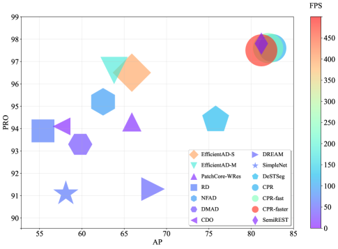
Figure 5: Inference speed (FPS) versus AP and PRO on MVTec AD benchmark. The algorithm speeds are indicated by the colors (the redder the faster) and sizes (the larger the faster) of the markers.

IV-E Qualitative Comparisons

In this section, qualitative AD results are shown for offering more intuitive understanding of the proposed method.

As a key step of CPR, the global retrieval procedure select the “similarly posed” reference images for the query. Figure 6 illustrate the retrieved $8$ nearest neighbors of a typical test image (inside the red rectangle) for each category. All the object categories in the MVTec AD dataset [58] are involved in this comparison except those sub-categories with well-aligned images. In Figure 6, our CPR method (top row) are compared with the SOTA image retrieval algorithm Unicom [75] (middle row) and RegAD [34] (bottow row) which is a SOTA AD approach employing STN layers for image alignment. Note that RegAD is not retreival-based and performs an implicit image alignment for each test image. As a result, we show the test image (inside the red rectangle) and $8$ randomly selected training images, all aligned using the affine transform parameters predicted by the STN layers of RegAD [34]. One can see that global retrieval process of CPR usually leads to a set of samples which seem “aligned” to the test image. In practice, this merit significantly benefits the proposed CPR algorithm for both training and inference. In contrast, the general retrieval algorithm Unicom [58] performs worse than CPR and the alignment-based RegAD [34] fails to align all the images to similar poses.

Figure 6: Global retrieval results on MVTec AD. The proposed GRB (top row) achieves more robust retrieval results for various categories of defective objects, comparing with the Unicom algorithm [75] (middle row) and the RegAD method [34] (bottom row). The images inside the red rectangles are the test images while the others are the retrieved $8$-NN images. Note that for RegAD, the $8$ training image are randomly selected and all the $9$ images are supposed to be aligned to similar poses according to the original paper [34].

Secondly, in Figure 7 we demonstrate the foreground estimation of the proposed FEB module. As it can be seen, the FEB can accurately predict the pixel labels (foreground vs. background) even though no manual annotation is available in the training stage.

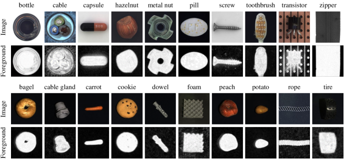
Figure 7: The demonstration of the proposed FEB module. All the object categories in MVTec AD (top row) and MVTec-3D AD (bottom row) are illustrated in this figure. Note that instead of the binary map, CPR utilizes the foreground confidence to reduce the influence of the “false alarms” in the background region.

Finally, the anomaly score maps of our method and $4$ representative AD algorithms are shown in Figure 8. As we can see from the image, CPR predicts more accurate score maps in most scenarios.

Figure 8: Visualization comparisons examples of anomaly localization on MVTec AD. Our method accurately localizes anomalous regions and shows more similar predictions to the ground truth.

V Conclusion & future work

In this paper, we rethink the inherent “matching” nature of anomaly detection and consequently propose to perform AD in a cascade manner. The former layer of the cascade filters out most improper reference images while the test patch is matched with the reference set in the latter layer. This coarse-to-fine retrieval strategy is proved to be remarkably useful and yields new SOTA AD accuracy as well as a running speed over $1000$ FPS with a moderate simplification. Besides the good performances, this work also sheds light on the understanding of all the matching-based AD algorithms. According to the empirical study of this work, the high accuracy usually stems from two crucial factors, namely the reference set selection and the metric feature learning. In the future, algorithms can be improved by finding more sophisticated alternatives to those two key components. In addition, the running speed of the retrieval-based AD process could be further increased by introducing the hashing techniques which have wide applications in fast retrieval.

References

- [1] B. Scholkopf, R. Williamson, A. Smola, J. Shawe-Taylor, J. Platt et al., “Support vector method for novelty detection,” Adv. Neural Inform. Process. Syst., vol. 12, no. 3, pp. 582–588, 2000.
- [2] B. Schölkopf, J. C. Platt, J. Shawe-Taylor, A. J. Smola, and R. C. Williamson, “Estimating the support of a high-dimensional distribution,” Neural computation, vol. 13, no. 7, pp. 1443–1471, 2001.
- [3] L. Ruff, N. Görnitz, L. Deecke, S. A. Siddiqui, R. A. Vandermeulen, A. Binder, E. Müller, and M. Kloft, “Deep one-class classification,” in AAAI Conference on Artificial Intelligence, ser. Proceedings of Machine Learning Research, vol. 80. PMLR, 2018, pp. 4390–4399.
- [4] J. Yi and S. Yoon, “Patch svdd: Patch-level svdd for anomaly detection and segmentation,” in ACCV, 2020.
- [5] P. Liznerski, L. Ruff, R. A. Vandermeulen, B. J. Franks, M. Kloft, and K. R. Muller, “Explainable deep one-class classification,” in Int. Conf. Learn. Represent., 2021.
- [6] F. V. Massoli, F. Falchi, A. Kantarci, Ş. Akti, H. K. Ekenel, and G. Amato, “Mocca: Multilayer one-class classification for anomaly detection,” IEEE Transactions on Neural Networks and Learning Systems, vol. 33, no. 6, pp. 2313–2323, 2022.
- [7] T. Defard, A. Setkov, A. Loesch, and R. Audigier, “Padim: A patch distribution modeling framework for anomaly detection and localization,” in Pattern Recognition. ICPR International Workshops and Challenges. Cham: Springer International Publishing, 2021, pp. 475–489.
- [8] K. Zhang, B. Wang, and C.-C. J. Kuo, “Pedenet: Image anomaly localization via patch embedding and density estimation,” Pattern Recognition Letters, vol. 153, pp. 144–150, 2022.
- [9] Y. Chen, Y. Tian, G. Pang, and G. Carneiro, “Deep one-class classification via interpolated gaussian descriptor,” in AAAI, vol. 36, no. 1, 2022, pp. 383–392.
- [10] L. Dinh, D. Krueger, and Y. Bengio, “Nice: Non-linear independent components estimation,” arXiv e-prints, vol. abs/1410.8516, 2014.
- [11] M. Rudolph, B. Wandt, and B. Rosenhahn, “Same same but differnet: Semi-supervised defect detection with normalizing flows,” in IEEE/CVF Winter Conference on Applications of Computer Vision, 2021, pp. 1907–1916.
- [12] J. Yu, Y. Zheng, X. Wang, W. Li, Y. Wu, R. Zhao, and L. Wu, “Fastflow: Unsupervised anomaly detection and localization via 2d normalizing flows,” arXiv e-prints, vol. abs/2111.07677, 2021.
- [13] M. Tailanian, Á. Pardo, and P. Musé, “U-flow: A u-shaped normalizing flow for anomaly detection with unsupervised threshold,” arXiv e-prints, vol. abs/2211.12353, 2022.
- [14] D. Gudovskiy, S. Ishizaka, and K. Kozuka, “Cflow-ad: Real-time unsupervised anomaly detection with localization via conditional normalizing flows,” in IEEE/CVF Winter Conference on Applications of Computer Vision, 2022, pp. 1819–1828.
- [15] J. Lei, X. Hu, Y. Wang, and D. Liu, “Pyramidflow: High-resolution defect contrastive localization using pyramid normalizing flow,” in IEEE Conf. Comput. Vis. Pattern Recog., 2023, pp. 14 143–14 152.
- [16] C.-L. Li, K. Sohn, J. Yoon, and T. Pfister, “Cutpaste: Self-supervised learning for anomaly detection and localization,” in IEEE Conf. Comput. Vis. Pattern Recog., 2021, pp. 9659–9669.
- [17] V. Zavrtanik, M. Kristan, and D. Skočaj, “DrÆm – a discriminatively trained reconstruction embedding for surface anomaly detection,” in Int. Conf. Comput. Vis., 2021, pp. 8310–8319.
- [18] M. Yang, P. Wu, and H. Feng, “Memseg: A semi-supervised method for image surface defect detection using differences and commonalities,” Engineering Applications of Artificial Intelligence, vol. 119, p. 105835, 2023.
- [19] M. Salehi, N. Sadjadi, S. Baselizadeh, M. H. Rohban, and H. R. Rabiee, “Multiresolution knowledge distillation for anomaly detection,” in IEEE Conf. Comput. Vis. Pattern Recog., 2021, pp. 14 902–14 912.
- [20] H. Deng and X. Li, “Anomaly detection via reverse distillation from one-class embedding,” in IEEE Conf. Comput. Vis. Pattern Recog., 2022, pp. 9727–9736.
- [21] P. Bergmann, K. Batzner, M. Fauser, D. Sattlegger, and C. Steger, “Beyond dents and scratches: Logical constraints in unsupervised anomaly detection and localization,” Int. J. Comput. Vis., vol. 130, no. 4, p. 947–969, 2022.
- [22] X. Zhang, S. Li, X. Li, P. Huang, J. Shan, and T. Chen, “Destseg: Segmentation guided denoising student-teacher for anomaly detection,” in IEEE Conf. Comput. Vis. Pattern Recog., 2023, pp. 3914–3923.
- [23] B. Zong, Q. Song, M. R. Min, W. Cheng, C. Lumezanu, D. Cho, and H. Chen, “Deep autoencoding gaussian mixture model for unsupervised anomaly detection,” in Int. Conf. Learn. Represent. OpenReview.net, 2018.
- [24] D. Dehaene and P. Eline, “Anomaly localization by modeling perceptual features,” arXiv e-prints, vol. abs/2008.05369, 2020.
- [25] Y. Shi, J. Yang, and Z. Qi, “Unsupervised anomaly segmentation via deep feature reconstruction,” Neurocomputing, vol. 424, pp. 9–22, 2021.
- [26] J. Hou, Y. Zhang, Q. Zhong, D. Xie, S. Pu, and H. Zhou, “Divide-and-assemble: Learning block-wise memory for unsupervised anomaly detection,” in Int. Conf. Comput. Vis., 2021, pp. 8791–8800.
- [27] J.-C. Wu, D.-J. Chen, C.-S. Fuh, and T.-L. Liu, “Learning unsupervised metaformer for anomaly detection,” in Int. Conf. Comput. Vis., 2021, pp. 4349–4358.
- [28] K. Roth, L. Pemula, J. Zepeda, B. Schölkopf, T. Brox, and P. Gehler, “Towards total recall in industrial anomaly detection,” in IEEE Conf. Comput. Vis. Pattern Recog., 2022, pp. 14 318–14 328.
- [29] D. Kim, C. Park, S. Cho, and S. Lee, “Fapm: Fast adaptive patch memory for real-time industrial anomaly detection,” arXiv e-prints, vol. abs/2211.07381, 2022.
- [30] J. Bae, J.-H. Lee, and S. Kim, “Image anomaly detection and localization with position and neighborhood information,” arXiv e-prints, vol. abs/2211.12634, 2022.
- [31] G. Xie, J. Wang, J. Liu, F. Zheng, and Y. Jin, “Pushing the limits of fewshot anomaly detection in industry vision: Graphcore,” arXiv e-prints, vol. abs/2301.12082, 2023.
- [32] R. Saiku, J. Sato, T. Yamada, and K. Ito, “Enhancing anomaly detection performance and acceleration,” IEEJ Journal of Industry Applications, vol. 11, no. 4, pp. 616–622, 2022.
- [33] H. Zhu, Y. Kang, Y. Zhao, X. Yan, and J. Zhang, “Anomaly detection for surface of laptop computer based on patchcore gan algorithm,” in 2022 41st Chinese Control Conference (CCC), 2022, pp. 5854–5858.
- [34] C. Huang, H. Guan, A. Jiang, Y. Zhang, M. Spratling, and Y.-F. Wang, “Registration based few-shot anomaly detection,” in Eur. Conf. Comput. Vis. Cham: Springer Nature Switzerland, 2022, pp. 303–319.
- [35] Y. Zheng, X. Wang, R. Deng, T. Bao, R. Zhao, and L. Wu, “Focus your distribution: Coarse-to-fine non-contrastive learning for anomaly detection and localization,” in Int. Conf. Multimedia and Expo. IEEE, 2022, pp. 1–6.
- [36] W. Liu, H. Chang, B. Ma, S. Shan, and X. Chen, “Diversity-measurable anomaly detection,” in IEEE Conf. Comput. Vis. Pattern Recog., 2023, pp. 12 147–12 156.
- [37] P. Bergmann, M. Fauser, D. Sattlegger, and C. Steger, “Mvtec AD - A comprehensive real-world dataset for unsupervised anomaly detection,” in IEEE Conf. Comput. Vis. Pattern Recog. Computer Vision Foundation / IEEE, 2019, pp. 9592–9600.
- [38] W. Chen, Y. Liu, W. Wang, E. M. Bakker, T. Georgiou, P. Fieguth, L. Liu, and M. S. Lew, “Deep learning for instance retrieval: A survey,” IEEE Trans. Pattern Anal. Mach. Intell., vol. 45, no. 6, p. 7270–7292, 2023.
- [39] Y. Kalantidis, C. Mellina, and S. Osindero, “Cross-dimensional weighting for aggregated deep convolutional features,” in Eur. Conf. Comput. Vis. Worksh. Springer, 2016, pp. 685–701.
- [40] J. Yue-Hei Ng, F. Yang, and L. S. Davis, “Exploiting local features from deep networks for image retrieval,” in IEEE Conf. Comput. Vis. Pattern Recog. Worksh., 2015, pp. 53–61.
- [41] J. Xu, C. Shi, C. Qi, C. Wang, and B. Xiao, “Unsupervised part-based weighting aggregation of deep convolutional features for image retrieval,” in AAAI. AAAI Press, 2018, pp. 7436–7443.
- [42] R. Arandjelovic, P. Gronát, A. Torii, T. Pajdla, and J. Sivic, “Netvlad: CNN architecture for weakly supervised place recognition,” in IEEE Conf. Comput. Vis. Pattern Recog. IEEE Computer Society, 2016, pp. 5297–5307.
- [43] A. Gordo, J. Almazán, J. Revaud, and D. Larlus, “Deep image retrieval: Learning global representations for image search,” in Eur. Conf. Comput. Vis. Springer, 2016, pp. 241–257.
- [44] F. Tan, J. Yuan, and V. Ordonez, “Instance-level image retrieval using reranking transformers,” in Int. Conf. Comput. Vis., 2021, pp. 12 085–12 095.
- [45] L. Zheng, S. Wang, J. Wang, and Q. Tian, “Accurate image search with multi-scale contextual evidences,” Int. J. Comput. Vis., vol. 120, no. 1, p. 1–13, 2016.
- [46] O. Morere, J. Lin, A. Veillard, L.-Y. Duan, V. Chandrasekhar, and T. Poggio, “Nested invariance pooling and rbm hashing for image instance retrieval,” in ACM International Conference on Multimedia Retrieval, 2017, pp. 260–268.
- [47] J. Song, T. He, L. Gao, X. Xu, and H. T. Shen, “Deep region hashing for efficient large-scale instance search from images,” arXiv e-prints, 2017.
- [48] H.-F. Yang, K. Lin, and C.-S. Chen, “Supervised learning of semantics-preserving hash via deep convolutional neural networks,” IEEE Trans. Pattern Anal. Mach. Intell., vol. 40, no. 2, pp. 437–451, 2018.
- [49] G. Tolias, Y. Avrithis, and H. Jégou, “Image search with selective match kernels: Aggregation across single and multiple images,” Int. J. Comput. Vis., vol. 116, no. 3, p. 247–261, 2016.
- [50] M. Teichmann, A. Araujo, M. Zhu, and J. Sim, “Detect-to-retrieve: Efficient regional aggregation for image search,” in IEEE Conf. Comput. Vis. Pattern Recog. Computer Vision Foundation / IEEE, 2019, pp. 5109–5118.
- [51] G. Huang, Z. Liu, L. van der Maaten, and K. Q. Weinberger, “Densely connected convolutional networks,” in IEEE Conf. Comput. Vis. Pattern Recog. IEEE Computer Society, 2017, pp. 2261–2269.
- [52] C. Szegedy, V. Vanhoucke, S. Ioffe, J. Shlens, and Z. Wojna, “Rethinking the inception architecture for computer vision,” in IEEE Conf. Comput. Vis. Pattern Recog. IEEE Computer Society, 2016, pp. 2818–2826.
- [53] R. Hadsell, S. Chopra, and Y. LeCun, “Dimensionality reduction by learning an invariant mapping,” in IEEE Conf. Comput. Vis. Pattern Recog., vol. 2, 2006, pp. 1735–1742.
- [54] H. Zhang, Z. Wu, Z. Wang, Z. Chen, and Y.-G. Jiang, “Prototypical residual networks for anomaly detection and localization,” in IEEE Conf. Comput. Vis. Pattern Recog., 2023, pp. 16 281–16 291.
- [55] Y. Wang, J. Peng, J. Zhang, R. Yi, Y. Wang, and C. Wang, “Multimodal industrial anomaly detection via hybrid fusion,” in IEEE Conf. Comput. Vis. Pattern Recog., 2023, pp. 8032–8041.
- [56] X. Yao, R. Li, J. Zhang, J. Sun, and C. Zhang, “Explicit boundary guided semi-push-pull contrastive learning for supervised anomaly detection,” in IEEE Conf. Comput. Vis. Pattern Recog., 2023, pp. 24 490–24 499.
- [57] P. Bergmann, X. Jin, D. Sattlegger, and C. Steger, “The MVTec 3D-AD Dataset for Unsupervised 3D Anomaly Detection and Localization,” arXiv e-prints, p. arXiv:2112.09045, 2021.
- [58] P. Bergmann, M. Fauser, D. Sattlegger, and C. Steger, “Mvtec AD - A comprehensive real-world dataset for unsupervised anomaly detection,” in IEEE Conf. Comput. Vis. Pattern Recog. Computer Vision Foundation / IEEE, 2019, pp. 9592–9600.
- [59] O. Russakovsky, J. Deng, H. Su, J. Krause, S. Satheesh, S. Ma, Z. Huang, A. Karpathy, A. Khosla, M. Bernstein et al., “Imagenet large scale visual recognition challenge,” Int. J. Comput. Vis., vol. 115, pp. 211–252, 2015.
- [60] I. Loshchilov and F. Hutter, “Decoupled weight decay regularization,” in Int. Conf. Learn. Represent. OpenReview.net, 2019.
- [61] P. Mishra, R. Verk, D. Fornasier, C. Piciarelli, and G. L. Foresti, “Vt-adl: A vision transformer network for image anomaly detection and localization,” in International Symposium on Industrial Electronics, 2021, pp. 01–06.
- [62] P. Bergmann, M. Fauser, D. Sattlegger, and C. Steger, “Uninformed students: Student-teacher anomaly detection with discriminative latent embeddings,” in IEEE Conf. Comput. Vis. Pattern Recog. IEEE, 2020, pp. 4182–4191.
- [63] T. Saito and M. Rehmsmeier, “The precision-recall plot is more informative than the roc plot when evaluating binary classifiers on imbalanced datasets,” PloS one, vol. 10, no. 3, p. e0118432, 2015.
- [64] C. Ding, G. Pang, and C. Shen, “Catching both gray and black swans: Open-set supervised anomaly detection,” in IEEE Conf. Comput. Vis. Pattern Recog., 2022, pp. 7378–7388.
- [65] N.-C. Ristea, N. Madan, R. T. Ionescu, K. Nasrollahi, F. S. Khan, T. B. Moeslund, and M. Shah, “Self-supervised predictive convolutional attentive block for anomaly detection,” in IEEE Conf. Comput. Vis. Pattern Recog., 2022, pp. 13 566–13 576.
- [66] Y. Cao, X. Xu, Z. Liu, and W. Shen, “Collaborative discrepancy optimization for reliable image anomaly localization,” IEEE Transactions on Industrial Informatics, pp. 1–10, 2023.
- [67] H. Li, J. Wu, H. Chen, M. Wang, and C. Shen, “Efficient anomaly detection with budget annotation using semi-supervised residual transformer,” 2023.
- [68] Z. Liu, Y. Zhou, Y. Xu, and Z. Wang, “Simplenet: A simple network for image anomaly detection and localization,” in IEEE Conf. Comput. Vis. Pattern Recog., 2023, pp. 20 402–20 411.
- [69] M. Rudolph, T. Wehrbein, B. Rosenhahn, and B. Wandt, “Asymmetric student-teacher networks for industrial anomaly detection,” in IEEE/CVF Winter Conference on Applications of Computer Vision, 2023, pp. 2592–2602.
- [70] G. Pang, C. Ding, C. Shen, and A. van den Hengel, “Explainable deep few-shot anomaly detection with deviation networks,” arXiv e-prints, vol. abs/2108.00462, 2021.
- [71] M. Tan and Q. V. Le, “Efficientnet: Rethinking model scaling for convolutional neural networks,” in AAAI Conference on Artificial Intelligence, ser. Proceedings of Machine Learning Research, vol. 97. PMLR, 2019, pp. 6105–6114.
- [72] S. Migacz, “8-bit inference with tensorrt,” in GPU technology conference, vol. 2, no. 4, 2017, p. 5.
- [73] A. Paszke, S. Gross, F. Massa, A. Lerer, J. Bradbury, G. Chanan, T. Killeen, Z. Lin, N. Gimelshein, L. Antiga, A. Desmaison, A. Köpf, E. Yang, Z. DeVito, M. Raison, A. Tejani, S. Chilamkurthy, B. Steiner, L. Fang, J. Bai, and S. Chintala, “Pytorch: An imperative style, high-performance deep learning library,” in Adv. Neural Inform. Process. Syst., 2019, pp. 8024–8035.
- [74] K. Batzner, L. Heckler, and R. König, “Efficientad: Accurate visual anomaly detection at millisecond-level latencies,” 2023.
- [75] X. An, J. Deng, K. Yang, J. Li, Z. Feng, J. Guo, J. Yang, and T. Liu, “Unicom: Universal and compact representation learning for image retrieval,” Int. Conf. Learn. Represent., 2023.