Yang-Gaudin model: A paradigm of many-body physics

Abstract

Using Bethe’s hypothesis, C N Yang exactly solved the one-dimensional (1D) delta-function interacting spin-1/2 Fermi gas with an arbitrary spin-imbalance in 1967. At that time, using a different method, M Gaudin solved the problem of interacting fermions in a spin-balanced case. Later, the 1D delta-function interacting fermion problem was named as the Yang-Gaudin model. It has been in general agreed that a key discovery of C N Yang’s work was the cubic matrix equation for the solvability conditions. This equation was later independently found by R J Baxter for commuting transfer matrices of 2D exactly solvable vertex models. The equation has since been referred to Yang-Baxter equation, being the master equation to integrability. The Yang-Baxter equation has been used to solve a wide range of 1D many-body problems in physics, such as 1D Hubbard model, $SU(N)$ Fermi gases, Kondo impurity problem and strongly correlated electronic systems etc. In this paper, we will briefly discuss recent developments of the Yang-Gaudin model on several breakthroughs of many-body phenomena, ranging from the universal thermodynamics to the Luttigner liquid, the spin charge separation, the Fulde-Ferrell-Larkin-Ovchinnikov (FFLO)-like pairing state and the quantum criticality. These developments demonstrate that the Yang-Gaudin model has laid out a profound legacy of the Yang-Baxter equation.

The Bethe ansatz (BA), i.e. a particular form of wavefunction, was first introduced in 1931 by Hans Bethe Bethe:1931 as a way to obtain the eigenspectrum of the one-dimensional (1D) spin-1/2 Heisenberg chain. In Bethe’s method, $N!$ plane waves are $N$-fold products of individual exponential phase factors $e^{\mathrm{i}k_{i}x_{j}}$, where the $N$ distinct wave numbers, $\left\{k_{i}\right\}$, are permuted among the $N$ distinct coordinates, $x_{j}$. Each of the $N!$ plane waves has an amplitude coefficient in each of regions, i.e. superposition of all possible plane waves of $N$ particles. However, only more than few decades later, physicists, L Hulthén Hulthen , R. Orbach Orbach , L R Walker Walker , R B Griffith Griffith , J des Cloizeaux and Pearson Cloizeau , and few others, studied the Bethe’s method and the Heisenberg chain in terms of Bethe’s solution. In the mid-60’s, C N Yang and C P Yang YY-1 ; YY-2 ; YY-3 presented a systematic study of the BA equations for the Heisenberg spin chain throughout the full range of anisotropic parameter $\Delta$ with a presence of magnetic field. While they coined Bethe’s method as Bethe’s hypothesis.

In 60’s, Bethe’s hypothesis had been proved to be invaluable for the field of exactly solvable models in statistical mechanics. In 1963, using Bethe’s hypothesis, E Lieb and W Liniger Lieb-Liniger solved the 1D Bose gas with a delta-function interaction. In 1967, C N Yang Yang solved the 1D delta-interacting Fermi gas with a discovery of the necessary condition for the Bethe ansatz solvability, which is now known as the Yang-Baxter equation, i.e. the factorization condition–the scattering matrix of a quantum many-body system can be factorized into a product of many two-body scattering matrices. In the same year, M Gaudin also rigorously derived the BA equations for the spin-$1/2$ Fermi gas with a spin balance Gaudin . In 1972, R J Baxter Baxter independently showed that such a factorization relation also occurred as the conditions for commuting transfer matrices in 2D vertex models in statistical mechanics. The Bethe ansatz approach has since found success in the realm of condensed matter physics, such as the 1D Hubbard model Lieb-Wu , SU(N) interacting Fermi gases Sutherland:1968 , Kondo impurity problems Andrei:1983 , BCS pairing models Dukelsky:2004 , strongly correlated electron systems 1D-Hubbard ; Korepin ; Sutherland-book ; Takahashi-b ; Wang-book and spin chain and ladder compounds Batchelor:2007 , quantum gases of cold atoms Cazalilla:2011 ; yangyou ; Guan:2013 ; Batchelor:2016 ; Mistakidis:2022 , and also many other problems in physics and mathematics.

The next significant progress was made by C N Yang and C P Yang Yang-Yang in 1969 on the finite temperature problem for the Lieb-Liniger Bose gas. They showed that the thermodynamics of the model can be determined from the minimisation conditions of the Gibbs free energy subject to the Bethe ansatz equations. Later Takahashi showed Takahashi:1971 ; Takahashi:1972 that the Yang-Yang method was an elegant way to analytically obtain thermodynamics of integrable models, e.g. 1D Heisenberg spin chains, Hubbard model, etc. Recent developments on the exactly solvable models in ultracold atoms have shown Guan:2013 ; Zhao ; Guan2007 ; Guan:2013PRL ; Yang:2017 ; He:2020 ; PhysRevB.101.035149 that Yang-Yang method provides an elegant way to study universal thermodynamics, Luttinger liquid, spin charge separation, transport properties and critical phenomena for a wide range of low-dimensional quantum many-body systems. In this short review, we shall discuss how the exact solution of the Yang-Gaudin model provides a rigorous understanding of such fundamental many-body physics in terms of the legacy of Yang-Baxter equation and Yang-Yang thermodynamics.

In this paper, we will present Bethe ansatz solution of the Yang-Guadin model in Section I and will discuss the ground state, spin charge separation, universal thermodynamics and quantum criticality for the model with a repulsive interaction in Section II. In section III, we will briefly review novel quantum phases of pairing and depairing, the Fulde-Ferrell-Larkin-Ovchinnikov (FFLO) pairing correlation, multicomponent Luttinger liquids and dimensionless ratios for the Yang-Gaudin model with an attractive interaction. A brief conclusion and a short discussion on the future study of the Yang-Gaudin model will be presented in Section IV.

I I. The Yang-Gaudin Model

The Hamiltonian for the 1D contact interacting fermion problem Yang ; Gaudin

$$H=-\frac{\hbar^{2}}{2m}\sum_{i=1}^{N}\frac{\partial^{2}}{\partial x_{i}^{2}}+g_{1D}\sum_{1\leq i<j\leq N}\delta(x_{i}-x_{j})$$ (1)

describes $N$ fermions of the same mass $m$ with two internal spin states confined to a 1D system of length $L$ interacting via a $\delta$-function potential. In this Hamiltonian, we denote the numbers of fermions in the two hyperfine levels $|\uparrow\rangle$ and $|\downarrow\rangle$ as $N_{\uparrow}$ and $N_{\downarrow}$, respectively. While we denoted the total number of fermions and the magnetization as $N=N_{\uparrow}+N_{\downarrow}$ and $M^{z}=(N_{\uparrow}-N_{\downarrow})/2$. The coupling constant $g_{1D}$ can be expressed in terms of the interaction strength $g_{1D}=\hbar^{2}c/m$ with $c=-2/a_{1D}$, where $a_{1D}$ is the effective 1D scattering length Olshanii_PRL_1998 . In the following discussion, we let $2m=\hbar=1$ for our convenience. We define a dimensionless interaction strength $\gamma=c/n$ for our later physical analysis. Here the linear density is defined by $n=N/L$. For a repulsive interaction, $c>0$ and for an attractive interaction, $c<0$.

Using Bethe’s hypothesis, C N Yang solved the model (1) with the following many-body wave function

$$\psi=\sum_{P}A_{\sigma_{1}\ldots\sigma_{N}}(P|Q)\exp\textrm{i}(k_{P1}x_{Q1}+\ldots+k_{PN}x_{QN})$$ (2)

for the domain $0<x_{Q1}<x_{Q2}<\ldots<x_{QN}<L$. Where $\{k_{i}\}$ denote a set of unequal wave numbers and $\sigma_{i}$ with $i=1,\ldots,N$ indicate the spin coordinates. Both $P$ and $Q$ are permutations of indices $\{1,2,\ldots,N\}$, i.e. $P=\left\{P_{1},\ldots,P_{N}\right\}$ and $Q=\left\{Q_{1},\ldots,Q_{N}\right\}$. The sum runs over all $N!$ permutations $P$ and the coefficients of the exponentials are column vectors with each of the $N!$ components representing a permutation $Q$. To determine the wave function associated with the irreducible representations of the permutation group $S_{N}$ and the irreducible representation of the Young tableau for different up- and down-spin fermions, one first needs to consider the boundary conditions of the wave function, i.e. the continuity of the wave function and discontiuity of its derivative. It follows that the two adjacent coefficients must meet the two-body scattering relation

$$A_{\sigma_{1}\ldots\sigma_{N}}(P_{i}P_{j}|Q_{i}Q_{j})=Y_{ij}(k_{Pj}-k_{Pi})A_{\sigma^{\prime}_{1}\ldots\sigma^{\prime}_{N}}(P_{j}P_{i}|Q_{i}Q_{j}),$$ (3)

where the two-body scattering matrix $Y_{ij}$ is given by

$$Y_{ij}(k_{Pj}-k_{Pi})=\left[\frac{\textrm{i}(k_{Pj}-k_{Pi})T_{ij}+cI}{\textrm{i}(k_{Pj}-k_{Pi})-c}\right]^{\sigma^{\prime}_{1}\ldots\sigma^{\prime}_{N}}_{\sigma_{1}\ldots\sigma_{N}}$$ (4)

with the operator $T_{ij}=-P_{ij}$, here $P_{ij}$ is the permutation operator.

The key discovery of C N Yang’s work is that the two-body scattering matrix acting on three linear tensor spaces $V_{1}\otimes V_{2}\otimes V_{3}$

$$Y_{ij}(u)=\frac{\textrm{i}uT_{ij}+cI}{\textrm{i}u-c}$$ (5)

satisfies the following cubic equation

$$Y_{12}(k_{2}-k_{1})Y_{23}(k_{3}-k_{1})Y_{12}(k_{3}-k_{2})$$

$$=Y_{23}(k_{3}-k_{2})Y_{12}(k_{3}-k_{1})Y_{23}(k_{2}-k_{1}),$$ (6)

which has been known as the Yang-Baxter equation. This equation guarantees no diffraction in the three-particle scattering process, i.e. $(k^{\prime}_{1},k^{\prime}_{2},k^{\prime}_{3})=(k_{1},k_{2},k_{3})$. The Yang-Baxter equation in a graphical representation presents a kind of topological invariance for interchanging the three operators according to the two paths, see Fig. 1. This equation was immediately seen as a necessary condition to the quantum integrability.

Figure 1: The graphical representation of the Yang-Baxter equation Eq. (6).

In general, the scattering matrix $Y_{ab}(u)$ satisfies the following relations

$$Y_{ab}(u)Y_{cd}(v) = Y_{cd}(v)Y_{ab}(u),$$

$$Y_{ab}(u)Y_{bc}(u+v)Y_{ab}(v) = Y_{bc}(v)Y_{ab}(u+v)Y_{bc}(u),$$

$$Y_{ab}(u)Y_{ba}(-u) = 1.$$

Let us further introduce the operator $R_{ij}=T_{ij}Y_{ij}$ which acts on the space $\prod_{n=1}^{N}\otimes V_{n}$. Then we define the following monodromy matrix:

$$\mathcal{T}_{N}(u)=L_{N}(k_{N}-u)\ldots L_{2}(k_{2}-u)L_{1}(k_{1}-u)$$ (7)

where $L_{i}(k_{i}-u)\equiv R_{i,a}(k_{i}-u)$. By taking a trance of the transfer matrix over the auxiliary space $a$, we have $\tau(u)=\textrm{Tr}_{a}(\mathcal{T}_{N}(u))$, then we have

$$\tau(u)|_{u=k_{i}}=\mathfrak{R}_{i}(k_{i}),$$ (8)

where

$$\mathfrak{R}_{i}(k_{i}) = R_{i+1,i}(k_{i+1}-k_{i})\ldots R_{N,i}(k_{N}-k_{i})R_{1,i}(k_{1}-k_{i})\ldots$$ (9)

$$\times R_{i-1,i}(k_{i-1}-k_{i}).$$

The above notations were borrowed from the quantum inverse scattering method which had been developed in the 1980’s by Faddeev and others Korepin .

Solving the eigenvalue problem of $N$ interacting particles (1) in a periodic box of length $L$, one needs to apply the periodic boundary condition

$$\psi(x_{1},\ldots,x_{i},\ldots,x_{N})=\psi(x_{1},\ldots,x_{i}+L,\ldots,x_{N}).$$ (10)

This is equivalent to solving the following eigenvalue problem

$$\mathfrak{R}_{i}(k_{i})A_{E}(P|Q)=\exp(\textrm{i}k_{i}L)A_{E}(P|Q)$$ (11)

with the transfer matrix $\mathfrak{R}_{i}(k_{i})$ given by (9). By some algebraic manipulations, the eigenvalue of the transfer matrix $\tau(u)=\textrm{Tr}_{a}(\mathcal{T}_{N}(u))$ can be straightforwardly obtained. Then one can obtain the following C N Yang’s Bethe ansatz equations (BAE) Yang for the Fermi gas

$${\rm e}^{ik_{j}L}=\prod_{\alpha=1}^{M}\frac{k_{j}-\lambda_{\alpha}+ic/2}{k_{j}-\lambda_{\alpha}-ic/2},$$ (12)

$$\prod_{j=1}^{N}\frac{\lambda_{\alpha}-k_{j}+ic/2}{\lambda_{\alpha}-k_{j}-ic/2}=-\prod_{\beta=1}^{M}\frac{\lambda_{\alpha}-\lambda_{\beta}+ic}{\lambda_{\alpha}-\lambda_{\beta}-ic},$$ (13)

with $j=1,2,\cdots,N$ and $\alpha=1,2,\cdots,M$. Here $M$ is the number of atoms with down-spins. The energy eigenspectrum is given in terms of the quasimomenta $\left\{k_{i}\right\}$ of the fermions via $E=\frac{\hbar^{2}}{2m}\sum_{j=1}^{N}k_{j}^{2}$. All quasimomenta $\left\{k_{i}\right\}$ are distinct and uniquely determine the wave function of model Eq.(2).

The fundamental physics of the model (1) can be in principle obtained by solving the transcendental Bethe ansatz equations (12) and (13). However, the difficulty with this interacting fermion problem lies in finding all the solutions to these Bethe ansatz equations. In the following discussion, we will briefly review recent breakthroughs in the study of the Bethe ansatz solutions of the Yang-Gaudin model (1).

II II. Spin Charge Separation and Spin Incoherent Liquid for the Repulsive Fermi Gas

Finding the solution of the Bethe ansatz equations (12) and (13) is cumbersome. In the thermodynamic limit, i.e., $L,N\to\infty$, $N/L$ is finite, the above Bethe ansatz equations can be written as the generalized Fredholm equations

$${\rho}(k) = \frac{1}{2\pi}+\int_{-B_{2}}^{B_{2}}a_{1}(k-\lambda){\sigma_{1}}(\lambda)d\lambda,$$ (14)

$${\sigma_{1}}(\lambda) = \int_{-B_{1}}^{B_{1}}a_{1}(\lambda-k){\rho}(k)dk$$ (15)

$$-\int_{-B_{2}}^{B_{2}}a_{2}(\lambda-\lambda^{\prime}){\sigma_{1}}(\lambda^{\prime})d\lambda^{\prime}.$$

The associated integration boundaries $B_{1}$, $B_{2}$ are determined by the relations

$$n: \equiv N/L=\int_{-B_{1}}^{B_{1}}{\rho}(k)dk,$$

$$n_{\downarrow}: \equiv N_{\downarrow}/L=\int_{-B_{2}}^{B_{2}}{\sigma_{1}}(k)dk,$$ (16)

where $n$ denotes the linear density while $n_{\downarrow}$ is the density of spin-down Fermions. In the above equations we introduced the quasimomentum distribution function $\rho(k)$ and distribution function of the spin rapidity $\sigma_{1}(\lambda)$ for the ground state. The boundary $B_{1}$ characterizes the Fermi point in the quasimomentum space whereas the boundary $B_{2}$ characterizes the spin rapidity distribution interval with respect to the polarization. They can be obtained by solving the equations given in (16). In the above equations, we denoted the kernel function by

$$a_{\ell}(x)=\frac{1}{2\pi}\frac{\ell c}{(\ell c/2)^{2}+x^{2}}.$$ (17)

The ground state energy per unit length is given by

$$E=\int_{-B_{1}}^{B_{1}}k^{2}{\rho}(k)dk.$$ (18)

The ground state energy for weak and strong interactions can be calculated directly from the integral forms of the Bethe ansatz equations (14) and (15), namely

$$E = \frac{1}{12}n^{3}\pi^{2}+\frac{1}{2}n^{2}c+O(c^{2}),\,\,{\rm for}\,c\ll 1,$$ (19)

$$E = \frac{n^{3}\pi^{2}}{3}\left[1-\frac{4\ln 2}{\gamma}+\frac{12(\ln 2)^{2}}{\gamma^{2}}-\frac{32(\ln 2)^{3}}{\gamma^{3}}\right.$$ (20)

$$\left.+\frac{8\pi^{2}\zeta(3)}{5\gamma^{3}}\right]+O(c^{-4})\,\,{\rm for}\,c\gg 1.$$

This is a good approximation for the spin-balanced Fermi gas with weakly and strongly repulsive interactions. More detailed study of the solutions of the BA equations was presented in Guan:PRA12 .

In general, for a repulsive interaction, the Bethe ansatz equations (12) and (13) only admit real roots in the charge degree of freedom $k_{j}$, whereas in the spin sector, the spin string states are given by

$$\lambda_{\alpha}^{n,j}=\lambda_{\alpha}^{n}+\frac{ic}{2}(n+1-2j),\quad j=1,2,\cdots,n,$$ (21)

which are called the length-$n$ spin strings. Such a spin structure comprises a rich magnetism like what the 1D Heisenberg spin chain has. Accordingly, the Bethe ansatz equations (12) and (13) with string hypothesis (21) reduce to the following two sets of BA equations associated with the quantum number $\{I_{j}\}$ and $\{J_{\alpha}^{n}\}$

$$k_{j}L=2\pi I_{j}-\sum_{n=1}^{\infty}\sum_{\alpha=1}^{M_{n}}\theta\left(\frac{2(k_{j}-\lambda_{\alpha}^{n})}{nc}\right),$$ (22)

$$\sum_{j=1}^{N}\theta\left(\frac{2(k_{j}-\lambda_{\alpha}^{n})}{nc}\right)=2\pi J_{\alpha}^{n}$$

$$+\sum_{m=1}^{\infty}\sum_{\beta=1}^{M_{m}}\Theta_{mn}\left(\frac{2(\lambda_{\alpha}^{n}-\lambda_{\beta}^{m})}{c}\right),\$$ (23)

where $j=1,2,\cdots,N$, $\alpha=1,2,\cdots,M_{n},\;n\geq 1$ and $M_{n}$ is the number of length-$n$ string, $\theta(x)=2\tan^{-1}(x)$, and the function $\Theta_{mn}(x)$ is defined by

$$\Theta_{mn}(x)=\left\{\begin{array}[]{rcl}&&\theta\left(\frac{x}{|n-m|}\right)+2\theta\left(\frac{x}{|n-m|+2}\right)+\cdots\\ &&+2\theta\left(\frac{x}{n+m-2}\right)+\theta\left(\frac{x}{m+n}\right),\,\,\text{for}\,\,n\neq m,\\ &&2\theta\left(\frac{x}{2}\right)+2\theta\left(\frac{x}{4}\right)+\cdots\\ &&+2\theta\left(\frac{x}{2n-2}\right)+\theta\left(\frac{x}{2n}\right),\quad\text{for}\quad n=m.\end{array}\right.$$ (28)

The quantum number $I_{j}$ for charge degree of freedom takes distinct integers (or half-odd integers) for even (odd) $\sum_{\alpha}M_{\alpha}$, explicitly

$$I_{j}\in\sum_{n=1}^{\infty}\frac{M_{n}}{2}+\mathbb{Z}.$$ (29)

The spin quantum number $J_{\alpha}^{n}$ are distinct integers (half-odd integers) for odd (even) $N-M_{m}$, which satisfy

$$J_{\alpha}^{n}\in\frac{N-M_{n}}{2}+\frac{1}{2}+\mathbb{Z},$$

$$|J_{\alpha}^{n}|\leq J_{+}^{n}=\frac{N}{2}-\sum_{m=1}^{n}mM_{m}-n\sum_{m=n+1}^{\infty}M_{m}+\frac{M_{n}}{2}-\frac{1}{2},$$

$$J_{\alpha}^{n}=-J_{+}^{n},-J_{+}^{n}+1,-J_{+}^{n}+2,\cdots,J_{+}^{n}-1,J_{+}^{n}.$$

The total momentum of the system is given by

$$K=\sum_{j=1}^{N}k_{j}=\frac{2\pi}{L}\left(\sum_{j=1}^{N}I_{j}+\sum_{\alpha=1}^{M_{n}}\sum_{n=1}^{\infty}J_{\alpha}^{n}\right).$$ (30)

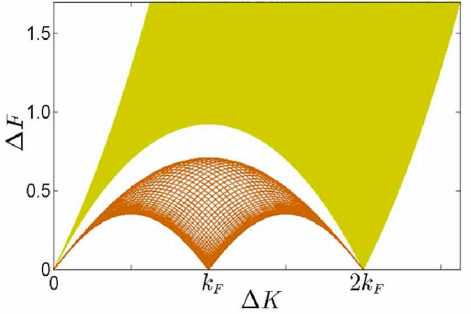
Figure 2: Exact low energy excitation spectra for charge (yellow green) and spin (dark brown) at $\gamma=5.03$ with the Fermi surface $k_{F}=n\pi$, density $n=N/L=3\times 10^{6}$. The yellow green spectrum shows the particle-hole continuum excitation. The dark brown spectrum shows the notable two-spinon excitation spectra. In long wave limit, i.e. $\Delta K\ll 1$, the spin and charge spectra show two independent linear dispersion with velocities $v_{s}$ and $v_{c}$, respectively. From He et. al. He:2020 .

It is significantly found He:2020 from the above Bethe ansatz equations (12) and (13) that the excitations in charge sector display a particle-hole continuum spectrum, see Fig. 2. It shows a linear dispersion structure for arbitrary strongly interacting fermions in a long wave limit

$$\omega(q)=v_{c}|q|\pm\frac{\hbar q^{2}}{2m^{*}}+\cdots,$$ (31)

where the charge velocity and the effective mass are given by the following expressions

$$v_{c} = \frac{\varepsilon_{c}^{\prime}(k_{0})}{2\pi\rho_{c}(k_{0})},$$ (32)

$$\frac{1}{2m^{*}} = \frac{\varepsilon_{c}^{\prime\prime}(k_{0})}{2(2\pi\rho_{c}(k_{0})^{2}}-\frac{\pi\rho_{c}^{\prime}(k_{0})\varepsilon_{c}^{\prime}(k_{0})}{(2\pi\rho_{c}(k_{0}))^{3}},$$ (33)

respectively. For a strong coupling limit, the charge velocity and the effective mass are given by He:2020

$$v_{c}\approx 2\pi n_{c}\left(1-\frac{4\ln 2}{\gamma}\right),\quad m^{*}=m\left(1+\frac{4\ln 2}{\gamma}\right).$$ (34)

The low-energy spin flipping excitation in the spin sector is also displayed in Fig. 2. It shows a typical two-spinon excitation spectrum in spin elementary excitations for the Yang-Gaudin model. The total excited momentum is given by

$$\Delta K_{\rm spinon}=n\pi-2\pi\sum_{j=1}^{2}\int_{0}^{\lambda_{j}^{\rm h}}\rho_{s}^{0}(\lambda){\rm d}\lambda,$$ (35)

while the energy of two-spinon excitation is given by

$$\Delta E_{\rm spinon}=-\sum_{j=1}^{2}\phi_{s}^{0}(\lambda_{j}^{\rm h}),$$ (36)

that present a microscopic origin of the two deconfined spinons with spin-$1/2$, showing a fractional excitation. This result confirms an antiferromagnetic ordering in the Fermi gas with internal degrees of freedom. However, when the interaction increases, the spin excitation band becomes lower, and even it vanishes in the limit $\gamma\to\infty$.

Moreover, Fig. 2 remarkably displays the origin of the separated excitations in spin and charge sectors. In fact, in one dimension such low-lying excitations with different sound velocities form two collective motions of bosons, i.e. the so-called spin-charge separation – fermions dissolve into spinons and holons. The spin-charge separation phenomenon is the hallmark of one-dimensional physics and has not been unambiguously confirmed by experiments, either in solids Kim:1996 ; auslaender2005spin ; Kim:2006 ; Jompol:2009 or ultracold atoms Hulet:2018 ; Vijayan:2020 . For theoretical understanding such unique 1D many-body phenomenon, it acquires low temperature thermodynamics and dynamical correlation functions for such excitations in spin and charge degrees of freedom. Such novel physics spin-charge separation has been recently observed with ultracold atoms in Senaratne:2021

On the other hand, the finite temperature problem for the Lieb-Liniger Bose gas was solved by C. N. Yang and C. P. Yang in 1969 Yang-Yang . Extension to the Yang-Gaudin model in terms of the Bethe ansatz equations (22) and (23) was done some time ago by Lai Lai:1971 ; Lai:1973 and M Takahashi Takahashi:1971 , namely, the so-called thermodynamic Bethe ansatz (TBA) equations for the Yang-Gaudin model are given by

$$\varepsilon(k) = k^{2}-\mu-\frac{H}{2}-T\sum_{n=1}^{\infty}a_{n}*{\rm ln}[1+{\rm e}^{-\phi_{n}(\lambda)/T}],\quad$$ (37)

$$\phi_{n}(\lambda) = nH-Ta_{n}*\ln[1+{\rm e}^{-\varepsilon(k)/T}]$$ (38)

$$+ T\sum_{m=1}^{\infty}T_{mn}*{\rm ln}[1+{\rm e}^{-\phi_{m}(\lambda)/T}]$$

with $n=1,\ldots,\infty$. Here $*$ denotes the convolution, $\varepsilon(k)$ and $\phi_{n}(\lambda)$ are the dressed energies for the charge and the length-$n$ spin strings, respectively, with $k$’s and $\lambda$’s being the rapidities; and the function $T_{mn}(x)=d\Theta_{mn}(x)/dx$ is given in Refs. Takahashi:1971 . The pressure is given by

$$p=\frac{T}{2\pi}\int_{-\infty}^{\infty}{\rm ln}[1+{\rm e}^{-\varepsilon(k)/T}]{\rm d}k,$$ (39)

from which all the thermal and magnetic quantities can be derived according to the standard statistical relations.

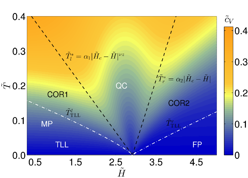
Figure 3: (color online) Contour plot of the dimensionless specific heat $\tilde{c}_{V}=c_{v}/T$, showing the phase diagram in the $\tilde{T}$-$\tilde{H}$ plane. Here dimensionless chemical potentials $\tilde{\mu}=2.5$, $\tilde{H}_{c}=2.9145$. The black dashed lines denote the peak positions of specific heat, whereas the white-dot-dashed line shows the boundary of the linear $T$ dependence of specific heat. $COR1$ denotes the crossover regions between QC and the TLL, giving a spin incoherent liquid. From He et. al. He:2020 .

At low temperatures, the TBA equations (37) and (38) are extremely hard to be solved either numerically or analytically. However, one can solve these coupled integral equations for certain physical regimes, for examples $k_{B}T\ll\mu,H$ or $c^{2}\gg E_{F}$, etc. For a fixed chemical potential, the contour plot of the specific heat in temperature-magnetic-field plane naturally reads off different critical regions near the quantum phase transition from the spin charge separated Tomonaga-Luttinger liquid (TLL) phase to a fully-polarized phase (FP), see Fig. 3. The quantum critical region fans out from the critical point, forming a critical cone.

For $T\ll E_{F}$, we can safely neglect the contributions from the high strings and just retain the leading length-1 string in the TBA equations (37) and (38). Throughout the TLL phase with $H<H_{c}$, where $H_{c}$ is the critical field for a fixed chemical potential

$$H_{c}=\left(\frac{c^{2}}{2\pi}+2\pi n^{2}\right)\tan^{-1}\left(\frac{2\pi n}{c}\right)-cn.$$ (40)

The pressure can, in general, be given by

$$p-p_{0}=\frac{\pi T^{2}}{6}\left(\frac{1}{v_{c}}+\frac{1}{v_{s}}\right),$$ (41)

where $p_{0}=\int_{-k_{0}}^{k_{0}}\varepsilon(k)dk$ is the pressure at $T=0$ and the charge and spin velocities are given by

$$v_{c}=\frac{t_{c}}{2\pi\rho(k_{0})}\,,\;\;\;\;v_{s}=\frac{t_{s}}{2\pi\sigma_{1}(\lambda_{0})}\,,$$ (42)

respectively, with $\rho$ and $\sigma_{1}$ being the distribution functions at Fermi points $k_{0}$ and $\lambda_{0}$ for the charge and the spin sectors, respectively. While $t_{c}=\frac{{\rm d}\varepsilon(k)}{{\rm d}k}\bigg{|}_{k=k_{0}}$ and $t_{s}=\frac{{\rm d}\phi_{1}(\lambda)}{{\rm d}\lambda}\bigg{|}_{\lambda=\lambda_{0}},$ are the respective linear slopes of the dispersion at the Fermi points. Although the proof of the form (41) is rather cumbersome, it gives a simple universal low temperature form of spin-charge separation theory Affleck1986 . The velocities can be numerically obtained for arbitrary interaction strength. For the strongly interacting regime, the charge and spin excitation velocities are given by

$$v_{c}\approx 2\pi n\left(1-\frac{4\ln 2}{\gamma}\right),\qquad v_{s}\approx\frac{2\pi^{3}n}{3\gamma}\left(1-\frac{6\ln 2}{\gamma}\right),$$

respectively. For the external field approaching the saturation field $H_{c}$, the charge and spin velocities can be derived from the relations (42). The leading terms in the velocities are then found to be

$$v_{c} = 2\pi n\left(1-\frac{12}{\pi\gamma}\sqrt{1-\frac{H}{H_{c}}}\right),\,\,v_{s}=\frac{H_{c}}{n}\sqrt{1-\frac{H}{H_{c}}}.$$

In the TLL regime, the dispersion relations for Yang-Gaudin model are approximately linear. Conformal field theory predicts that the energy per unit length has a universal finite size scaling form $E=E_{0}+\Delta/L^{2}$ where $E_{0}$ is the ground state energy per unit length for the infinite system and $\Delta$ is a universal term. In this scenario, Cardy Cardy1986 showed that the two-point correlation function between primary fields can be directly derived from conformal mapping using transfer matrix techniques and expressed the conformal dimensions in terms of finite-size corrections to the energy spectrum. For example, at zero temperature and zero magnetic field, by using conformal field theory Belavin1984 ; Blote1986 , the asymptotic of single particle correlation function can be given explicitly

$$G_{\uparrow}(x,t)\sim\langle\psi_{\uparrow}^{\dagger}(x,t)\psi_{\uparrow}(0,0)\rangle$$

$$\approx\frac{A_{\uparrow,1}e^{-\mathrm{i}k_{F\uparrow}x}}{(x-\mathrm{i}v_{c}t)^{2\Delta_{c}^{+}}(x+\mathrm{i}v_{c}t)^{2\Delta_{c}^{-}}(x-\mathrm{i}v_{s}t)^{2\Delta_{s}^{+}}}+h.c.$$ (43)

with the conformal dimensions

$$2\Delta_{c}^{+} = \frac{9}{16}-\frac{3\ln 2}{4\gamma}+\frac{3}{2\pi^{2}}\left(\frac{H}{H_{c}}\right)+\frac{3}{2\gamma}\left(\frac{H}{H_{c}}\right)$$ (44)

$$-\frac{\ln 2}{\pi^{2}\gamma}\left(\frac{H}{H_{c}}\right),$$

$$2\Delta_{c}^{-} = \frac{1}{16}-\frac{3\ln 2}{4\gamma}-\frac{1}{2\pi^{2}}\left(\frac{H}{H_{c}}\right)+\frac{1}{2\gamma}\left(\frac{H}{H_{c}}\right)$$ (45)

$$+\frac{3\ln 2}{\pi^{2}\gamma}\left(\frac{H}{H_{c}}\right),$$

$$2\Delta_{s}^{+} = \frac{1}{2}-\frac{2}{\pi^{2}}\left(\frac{H}{H_{c}}\right)-\frac{1}{\gamma}\left(\frac{H}{H_{c}}\right)+\frac{4\ln 2}{\pi^{2}\gamma}\left(\frac{H}{H_{c}}\right).$$ (46)

We see clearly that the correlation function decays as some power of distance governed by the critical exponent.

On the other hand, universal scaling behaviour can be derived in the vicinity of the critical point at low temperatures. Near the critical point, the spin dressed energy $\phi_{1}(\lambda)$ in (38) only has a small negative part, which makes a major contribution to the spin dressed energy near the critical point at low temperatures. Therefore, we can expand the integration kernel $a_{n}(k-\lambda)$ in terms of the functions of small variables $\lambda$. After a tedious calculation, we obtain the pressure of the Yang-Gaudin model (1) near the phase transition from the TLL phase to FP phase

$$p \approx p_{0}-\frac{\arctan\left(\frac{2}{c}k_{0}\right)T^{3/2}}{\pi^{3/2}\sqrt{(a+c_{2})}}\operatorname{Li}_{\frac{3}{2}}\left(-{\rm e}^{\frac{s_{0}\Delta H-c_{1}}{T}}\right)$$ (47)

$$+\frac{T^{5/2}}{4\pi^{3/2}(a+c_{2})^{3/2}}\frac{ck_{0}}{\left(c^{2}/4+k_{T}^{2}\right)^{2}}\operatorname{Li}_{\frac{5}{2}}\left(-{\rm e}^{\frac{s_{0}\Delta H-c_{1}}{T}}\right),$$

where the regular part $p_{0}$ of the pressure is given by

$$p_{0}=\frac{\pi T^{2}}{6v_{c}}+\frac{2}{3\pi}\left(\mu_{c}+\frac{H}{2}\right)^{3/2}=p_{0}^{\rm Liquid}+p_{0}^{\rm BG}.$$ (48)

The above expression $p_{0}^{\rm BG}=\frac{2}{3\pi}\left(\mu_{c}+\frac{H}{2}\right)^{3/2}$ can be regarded as the background part of charge, whereas $p_{0}^{\rm Liquid}=\frac{\pi T^{2}}{6v_{c}}$ denotes the Luttinger liquid contribution from charge degrees of freedom. However, the Luttinger liquid in the spin sector dissolves into the free fermion quantum criticality in the quantum critical (QC) region, see Fig. 3. It is worth noting that in the QC region the pressure (47) presents a universal scaling form of the equation of states

$$p=p_{0}^{\rm Liquid}+p_{0}^{\rm BG}+T^{\frac{1}{z}+1}\mathcal{G}\left(\frac{s_{0}\Delta H}{T^{1/\nu z}}\right),$$ (49)

from which one reads off the dynamical critical exponent $z=2$ and correlation length critical exponent $\nu=1/2$. Consequently, the scaling functions of all thermodynamic quantities can be derived based on this exact expression of the equation of states. The two crossover temperatures of the QC region are given by $T_{l}^{*}=\alpha_{1}|H-H_{c}|^{\nu z}$ and $T_{r}^{*}=\alpha_{2}|H-H_{c}|$, here $\alpha_{1,2}=s_{0}/y_{1,2}$ with $y_{1}=-1.5629$, $y_{2}=3.6205$ are numerical constants. In the QC region, all thermodynamic quantities can be cast into universal scaling forms.

In Fig. 3, we also identify a crossover region COR1 in the region $E_{\rm spin}\ll k_{B}T\ll E_{F}$. Here $E_{\rm spin}$ and $E_{F}$ are the energy of spin sector and Fermi energy, respectively. In this region, the interplay between the spin and the charge degrees of freedom leads to a large deviation from the linear dispersion in the spin sector, leading to a large disruption of the spin charge coherent TLLs. Consequently, the spin-spin correlation function exponentially decays, while the charge-charge correlation still remains power law decay with distance. Breakdown of the conformal field theory gives rise to an asymptotic of single particle correlation function

$$G_{\uparrow}(x,t) \approx \frac{A_{\uparrow,1}e^{-\mathrm{i}k_{F\uparrow}x}}{(x-\mathrm{i}v_{c}t)^{2\Delta_{c}^{+}}(x+\mathrm{i}v_{c}t)^{2\Delta_{c}^{-}}}$$ (50)

$$\times\frac{(\pi T/v_{s})^{2\Delta^{+}_{s}}}{e^{\frac{2\pi T}{v_{s}}x{\Delta_{s}^{+}}}}+h.c.$$

The conformal dimensions can be given by Eqs. (44)-(46). In this regime, the temperature is low enough in comparison with the Fermi energy, whereas it is high enough in comparison with the spin excitation energy. Therefore the spin velocity $v_{s}\to 0$ in this crossover region COR1, which is a reminiscence of the spin incoherent liquid Fiete:2007 ; Cheianov:2004 .

The novel phase diagram of Fig. 3 reveals a key concept that the low-lying excitations near the Fermi points dissolve into two separate collective motions of charge and spin, i.e., TLLs of charge and spin. Evidence for the spin-charge separation was reported in solid state materials. but none of those existing experiments in this study seemed to provide a conclusive observation of the spin-charge separated Luttinger liquids. In a recent experiment with ultracold atoms presented a confirmative observation of this phenomenon through the spin and charge dynamic structure factors Senaratne:2021 .

III III. FFLO Pairing Correlation and Universal Thermodynamics for the Attractive Fermi Gas

For the attractive regime, i.e. $c<0$, the root patterns of the BA equations (12) and (13) are significantly different from that of the model for $c>0$. For an attractive interaction, the quasimomenta $\left\{k_{i}\right\}$ of the fermions with different spins form two-body bound states Takahashi-a ; Gu-Yang , i.e., $k_{i}=\lambda_{i}\pm\mathrm{i}\frac{1}{2}c$, accompanied by the real spin parameter $\lambda_{i}$. Here $i=1,\ldots,N_{\downarrow}$. The excess fermions have real quasimomenta $\left\{k_{j}\right\}$ with $j=1,\ldots,N-2N_{\downarrow}$. Thus the Bethe ansatz equations for the ground state are transformed into the Fredholm equations according to the densities of the pairs $\rho_{2}(k)$ and density of single fermionic atoms $\rho_{1}(k)$. They satisfy the following Fredholm equations Yang ; Takahashi-a

$$\rho_{1}(k) = \frac{1}{2\pi}+\int_{-Q_{2}}^{Q_{2}}a_{1}(k-\lambda)\rho_{2}(\lambda)d\lambda,$$ (51)

$$\rho_{2}(\lambda) = \frac{2}{2\pi}+\int_{-Q_{1}}^{Q_{1}}a_{1}(\lambda-k^{\prime})\rho_{1}(k^{\prime})dk^{\prime}$$ (52)

$$+\int_{-Q_{2}}^{Q_{2}}a_{2}(\lambda-\lambda^{\prime})\rho_{2}(\lambda^{\prime})d\lambda^{\prime}$$

with the integration boundaries $Q_{1}$ and $Q_{2}$, which are the Fermi points of the single particles and pairs, respectively. Here $Q_{1}$ and $Q_{2}$ can be determined by the conditions

$$n \equiv: \frac{N}{L}=2\int_{-Q_{2}}^{Q_{2}}\rho_{2}(k)dk+\int^{Q_{1}}_{-Q_{1}}\rho_{1}(k)dk,$$

$$n_{\downarrow} \equiv: \frac{N_{\downarrow}}{L}=\int_{-Q_{2}}^{Q_{2}}\rho_{2}(k)dk.$$ (53)

The ground state energy per length is given by

$$E=\int_{-Q_{2}}^{Q_{2}}\left(2k^{2}+E_{B}\right)\rho_{2}(k)dk+\int_{-Q_{1}}^{Q_{1}}k^{2}\rho_{1}(k)dk.$$ (54)

In the above equation, the binding energy is given by $E_{B}=c^{2}/2$.

For an attractive interaction, there exist two Fermi seas in charge degree of freedom at the ground state. So that the Fermi points $Q_{1}$ and $Q_{2}$ are finite. This allows us to asymptotically solve the BA equations (51) and (52). For weak and strong attractions with an arbitrary polarization $P=(n_{\uparrow}-n_{\downarrow})/(n_{\uparrow}+n_{\downarrow})$, the ground state energy are respectively given by Guan:PRA12

$$E = \frac{1}{3}n_{\uparrow}^{3}\pi^{2}+\frac{1}{3}n_{\downarrow}^{3}\pi^{2}-2|c|n_{\uparrow}n_{\downarrow}+O(c^{2}),$$ (55)

$$E \approx \frac{\hbar^{2}n^{3}}{2m}\left\{-\frac{(1-P)\gamma^{2}}{4}+\frac{\pi^{2}(1-3P+3P^{2}+15P^{3})}{48}\right.$$ (56)

$$\left.+\frac{\pi^{2}(1-P)(1+P-5P^{2}+67P^{3})}{48|\gamma|}\right.$$

$$\left.+\frac{\pi^{2}(1-P)^{2}(1+5P+3P^{2}+247P^{3})}{64\gamma^{2}}\right.$$

$$\left.-\frac{\pi^{2}(1-P)}{1440|\gamma|^{3}}\left[-15+31125{P}^{4}+1861{\pi}^{2}{P}^{5}\right.\right.$$

$$\left.\left.-15765P^{5}-659{\pi}^{2}{P}^{4}+346{\pi}^{2}{P}^{3}-14{\pi}^{2}{P}^{2}\right.\right.$$

$$\left.\left.+\pi^{2}P+{\pi}^{2}-105P-150P^{2}-15090P^{3}\right]\right\},$$

respectively. This result was also obtained from dressed energy equations Guan2007 ; Wadati . We notice that the energy (55) continuously connects to the repulsive ground state energy (19) at $c\to 0$. But this does not mean that the energy analytically connects because of the divergence in the small region $c\to\mathrm{i}0$, see a discussion Guan:FP ; Takahashi:1970-m .

At finite temperatures, except the two-body bound states $k_{j}=\lambda_{j}\pm\mathrm{i}\frac{1}{2}c$ in charge sector, the spin quasimomenta of the BA equations (12) and (13) form complex strings $\lambda_{\alpha,j}^{n}=\lambda^{n}_{\alpha}+\mathrm{i}\frac{1}{2}(n+1-2j)c$ with $j=1,\ldots,n$ Takahashi:1971 ; Guan2007 . Here $\alpha=1,\ldots,N_{n}$ is the number of strings. The equilibrium states are determined by the minimization condition of the Gibbs free energy, which gives rise to a set of coupled nonlinear integral equations. In terms of the dressed energies $\epsilon_{2}(k):=T\ln(\rho_{2}^{h}(k)/\rho_{2}(k))$ and $\epsilon_{1}(k):=T\ln(\rho_{1}^{h}(k)/\rho_{1}(k))$ for paired and unpaired fermions Takahashi:1971 ; Guan2007 ; Schlottmann:1993 , the thermodynamic Bethe ansatz equations for the 1D attractive Fermi gas are given by

$$\epsilon_{2}(k) = 2(k^{2}-\mu-\frac{1}{4}{c^{2}})+Ta_{2}*\ln(1+\mathrm{e}^{-\epsilon_{2}(k)/T})$$

$$+\,Ta_{1}*\ln(1+\mathrm{e}^{-\epsilon_{1}(k)/{T}}),$$

$$\epsilon_{1}(k) = k^{2}-\mu-\frac{1}{2}{H}+Ta_{1}*\ln(1+\mathrm{e}^{-\epsilon_{2}(k)/{T}})$$

$$-T\sum_{n=1}^{\infty}a_{n}*\ln(1+\eta_{n}^{-1}(k)),$$

$$\ln\eta_{n}(\lambda) = \frac{nH}{T}+a_{n}*\ln(1+\mathrm{e}^{-\epsilon_{1}(\lambda)/{T}})$$ (57)

$$+\sum_{n=1}^{\infty}T_{mn}*\ln(1+\eta^{-1}_{n}(\lambda)),$$

where $n=1,\ldots,\infty$ and the function $\eta_{n}(\lambda):=\xi^{h}(\lambda)/\xi(\lambda)$ is the ratio of the string densities. While the function $T_{mn}(\lambda)$ is given in Takahashi:1971 ; Guan2007 . The Gibbs free energy per unit length, i.e. the pressure, is given by

$$p = \frac{T}{\pi}\int_{-\infty}^{\infty}dk\ln(1+\mathrm{e}^{-\epsilon_{2}(k)/{T}})$$ (58)

$$+\,\frac{T}{2\pi}\int_{-\infty}^{\infty}dk\ln(1+\mathrm{e}^{-\epsilon_{1}(k)/{T}}).$$

This serves as the equation of states, from which all the thermal and magnetic quantities can be derived according to the standard statistical mechanic relations.

From the TBA equations (57), at low temperatures, the pressure of the attractive Fermi gas with a strong interaction can be written as a sum of two components: $p=p_{1}+p_{2}$, where $p_{1}$ is the pressure for unpaired fermions and $p_{2}$ for pairs, given explicitly in Guan:2011-QC

$$p_{1}=F^{1}_{\frac{3}{2}}\left[1+\frac{p_{2}}{4|c|^{3}}\right],\,p_{2}=F^{2}_{\frac{3}{2}}\left[1+\frac{4p_{1}}{|c|^{3}}+\frac{p_{2}}{4|c|^{3}}\right],$$ (59)

respectively. Here $F^{r}_{a}=-\sqrt{{r}/{4\pi}}T^{a}{\rm Li}_{a}[-\exp({A_{r}/T})]$ ($r=1,2$) with $A_{1}=\mu_{1}-\frac{2p_{2}}{|c|}+\frac{1}{4|c|^{3}}F^{2}_{\frac{5}{2}}+Te^{-\frac{H}{T}}e^{-\frac{J}{T}}I_{0}\left(\frac{J}{T}\right)$ and $A_{2}=2\mu_{2}-\frac{4p_{1}}{|c|}-\frac{p_{2}}{|c|}+\frac{8}{|c|^{3}}F^{1}_{\frac{5}{2}}+\frac{1}{4|c|^{3}}F^{2}_{\frac{5}{2}}$. In the above equations $\mathrm{Li}_{n}(x)=\sum_{k=1}^{\infty}{x^{k}}/{k^{n}}$ is the polylogarithm function, $J=2p_{1}/|c|$ and $I_{0}(x)=\sum_{k=0}^{\infty}\left(x/2\right)^{2k}/{(k!)^{2}}$. This is a remarkable result of the low temperature thermodynamics of the Yang-Gaudin model Guan:2011-QC . Based on this result, the exact results of quantum criticality of the attractive Yang-Gaudin model can be found in Guan:2011-QC ; Yin:2011 ; Chen:2014 ; He-WB:2016 .

Figure 4: (Color online) Contour plot of the susceptibility Wilson ratio $R_{W}^{\chi}$ (60) of the attractive Fermi gas for dimensionless interaction $|\gamma|=10$. In this figure the reduced temperature $t=T/\varepsilon_{b}$ was used. $\varepsilon_{b}$ denotes the binding energy. The susceptibility Wilson ratio is temperature independent in the FFLO-like phase The dashed lines indicate the crossover temperature $T^{*}=\alpha|H-H_{c}|$ separating the relativistic TLL liquid from the free fermion quantum criticality. $R_{W}=0$ for both the TLL of pairs (PP) and the TLL of excess fermions (F). From Guan et. al., Guan:2013PRL .

A significant feature of the Yang-Gaudin model with an attractive interaction is the existence of the FFLO pairing state Larkin1965 ; Fulde1964 ; Yang2001 . The FFLO physics in Yang-Gaudin model has received extensive study in theory Orso ; HuiHu ; Feiguin2007 ; Rizzi2008 ; Zhao2008 ; Lee2011 ; Schlottmann2012 and experiment Liao ; Revelle:2016 . In 2007, three groups Guan2007 ; Orso ; HuiHu predicted the phase diagram of the attractive Fermi gas where the novel FFLO-like pairing phase sits in a large parameter space. The phase diagram can be mapped out from specific heat or dimensionless ratios, such as Grüneisen parameter Peng:2019 ; Yu:2020 , Wilson ratios Guan:2013PRL ; Yu:2016 . The dimensionless susceptibility $\chi$ and compressibility $\kappa$ Wilson ratios are given by

$$R_{W}^{\chi}=\frac{4}{3}\left(\frac{\pi k_{B}}{g\mu_{B}}\right)^{2}\frac{\chi}{c_{V}/T},\quad R_{W}^{\kappa}=\frac{\pi^{2}}{3}\frac{\kappa}{c_{V}/T}$$ (60)

that map out the phase diagram of the model in low temperature limit Guan:2013PRL ; Yu:2016 .

It is very interesting to note Guan:2013PRL ; Yu:2016 that additivity rules of thermodynamical properties within subsystems of the FFLO-like phase are a reminiscence of the rules for multi-resistor networks in series and parallel. Such simple additivity rules indicate a novel and useful characteristic of multi-component TLLs regardless of microscopic details of the systems. For the $SU(2)$ Fermi gas (1) with an attraction, we have the relations $H/2=\left({\mu}_{1}-{\mu}_{2}\right)+E_{B}/2$ and $n=2n_{2}+n_{1}$. Thus we may define the susceptibilities of subsystems in the FFLO state $\chi_{1}=(\mu_{\rm B}{g}_{\mathrm{Lande}})^{2}\left({\partial n_{1}}/{\partial\mu_{1}}\right)_{n}$, $\chi_{2}=2(\mu_{\rm B}{g}_{\mathrm{Lande}})^{2}\left({\partial n_{2}}/{\partial\mu_{2}}\right)_{n}$, and the compressibility $\kappa_{1}=\left({\partial n_{1}}/{\partial\mu_{1}}\right)_{H}$ and $\kappa_{2}=2\left({\partial n_{2}}/{\partial\mu_{2}}\right)_{H}$ in the grand canonical ensemble. Here $\mu_{B}$ is the Bohr magneton and $g_{\mathrm{Lande}}$ is the Lande factor. Consequently, the compressibility and susceptibility satisfy the following additivity rules

$$\kappa = \kappa_{1}+\kappa_{2},$$ (61)

$$\frac{1}{\chi} = \frac{1}{\chi_{1}}+\frac{1}{\chi_{2}}.$$ (62)

The compressibilities and susceptibilities are given explicitly in units of $\hbar^{2}/(2m)$

$$\kappa_{\mathrm{2}}^{-1} \approx \frac{\pi^{2}n_{2}}{4}\left(1+\frac{6n_{1}}{|c|}+\frac{4n_{2}}{|c|}+\frac{n_{2}^{2}}{2|c|n_{1}}+\frac{24n_{1}^{2}}{c^{2}}\right.$$ (63)

$$\left.+\frac{24n_{1}n_{2}}{c^{2}}+\frac{17n_{2}^{2}}{c^{2}}-\frac{2n_{2}^{3}}{c^{2}n_{1}}+\frac{n_{2}^{4}}{4c^{2}n_{1}^{2}}\right),$$

$$\kappa_{\mathrm{1}}^{-1} \approx 2\pi^{2}n_{1}\left(1+\frac{12n_{2}}{|c|}+\frac{16n_{1}^{2}}{|c|n_{2}}+\frac{96n_{2}^{2}}{c^{2}}+\frac{384n_{1}^{2}}{c^{2}}\right.$$ (64)

$$\left.-\frac{8n_{1}n_{2}}{c^{2}}-\frac{96n_{1}^{3}}{c^{2}n_{2}}+\frac{256n_{1}^{4}}{c^{2}n_{2}}\right)$$

and

$$\chi_{1}^{-1} = \pi^{2}n_{2}\left[1+\frac{4}{|c|}(n-3n_{2})+\frac{3}{c^{2}}(4n^{2}\right.$$ (65)

$$\left.-24nn_{2}+30n_{2}^{2})\right],$$

$$\chi_{2}^{-1} = 8\pi^{2}n_{1}\left[1+\frac{4}{|c|}(n-2n_{1})+\frac{4}{c^{2}}(2n^{2}\right.$$ (66)

$$\left.+10n_{1}^{2}-12nn_{1})\right].$$

Moreover, the interaction effect is revealed from the sound velocities $v_{1}$, $v_{2}$ of the excess fermions and bound pairs, for example, for strong attraction

$$v_{1} \approx \frac{\hbar}{2m}2\pi n_{1}\left(1+8n_{2}/|c|+48n_{2}^{2}/c^{2}\right),$$

$$v_{2} \approx \frac{\hbar}{2m}\pi n_{2}\left(1+2A/|c|+3A^{2}/c^{2}\right),$$ (67)

with $A=2n_{1}+n_{2}$. We similarly find that the specific heat satisfies

$$c_{V}=c_{V,1}+c_{V,2},$$ (68)

where $c_{V,r}=\frac{\pi k_{B}^{2}T}{3\hbar}\frac{1}{v_{r}}$ with $r=1,\,2$. It is remarkably observed that such additivity rules of compressibility (61), susceptibility (62) and the rescaled specific heat $c_{V}/T$ with (68) do not depend on the temperature in the FFLO-like state below a certain temperature. Such additivity rules are a characteristic of multi-component TLLs Yu:2016 . This nature presents a universal feature of thermodynamics for a two-component TLLs of pairs and single fermions in 1D.

Moreover, it was proved Yu:2016 that the susceptibility and compressibility Wilson ratios

$$R^{\chi}_{\mathrm{W},r^{\prime}} = \left(\sum_{r=1}^{2}\frac{D_{r}^{\chi}}{r^{2}}\right)^{-1}\left(\sum_{r=1}^{2}\frac{1}{v_{r}}\right)^{-1},$$ (69)

$$R^{\kappa}_{\mathrm{W}} = \left(\sum_{r=1}^{2}\frac{r^{2}}{D_{r}^{\kappa}}\right)\left(\sum_{r=1}^{2}\frac{1}{v_{r}}\right)^{-1}.$$ (70)

are dimensionless and uniquely determined by the sound velocities and stiffnesses. In the above expressions, the individual stiffnesses $D^{\kappa}_{r}$ and $D^{\chi}_{r}$ can be respectively given in terms of $\kappa_{r}$ and $\chi_{r}$ via

$$D_{r}^{\kappa} = \frac{r^{2}}{\pi\hbar}\frac{1}{\kappa_{r}},\qquad D_{r}^{\chi}=\frac{r^{2}}{\pi\hbar}\frac{1}{\chi_{r}}.$$ (71)

In this context the Wilson ratios of the Yang-Gaudin model with polarization elegantly determine the TLL nature of the FFLO-like state, see Fig. 4. It also indicates a universal feature of the quantum criticality of the attractive Fermi gas.

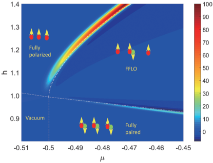
Figure 5: Contour plot of the negative Grüneisen parameter (72), i.e. $-\Gamma$, mapping out the full phase diagram of the Yang-Gaudin model with an attractive interaction in $h-\mu$ plane, see the main text. Here we set the dimensionless temperature $t=0.001$. From Yu, et. al. Yu:2020 .

On the other hand, Grüneisen parameter Gruneisen_AdP_1908 , which was introduced in the beginning of 20th century in the study of the effect of volume change of a crystal lattice on its vibrational frequencies, has been extensively studied for the exploration of the caloric effect of solids and phase transitions associated with volume change. Recently, one of the authors of this paper and coworkers Peng:2019 ; Yu:2020 studied interaction- and chemical potential-driven caloric effects and Grüneisen parameter in ultracold atomic gases in 1D. By using the Maxwell’s relations , the Grüneisen parameter of quantum gases in grand canonical ensemble is given by Yu:2020

$$\Gamma=V\frac{\left.\frac{\mathrm{d}p}{\mathrm{d}T}\right|_{V,N}}{\left.\frac{\mathrm{d}E}{\mathrm{d}T}\right|_{V,N}}=\frac{1}{T}\frac{\frac{\partial^{2}p}{\partial\mu^{2}}\frac{\partial p}{\partial T}-\frac{\partial^{2}p}{\partial\mu\partial T}\frac{\partial p}{\partial\mu}}{\frac{\partial^{2}p}{\partial\mu^{2}}\frac{\partial^{2}p}{\partial T^{2}}-\left(\frac{\partial^{2}p}{\partial\mu\partial T}\right)^{2}},$$ (72)

that remarkably maps out the phase diagram of the Yang-Gaudin model with an attractive interaction, see Fig. 5. This is intimately related to the expansionary caloric effect

$$\left.\frac{\partial T}{\partial V}\right|_{S,N,H} = \frac{T}{V}\Gamma.$$ (73)

Similarly one can find

$$\left.\frac{\partial T}{\partial H}\right|_{S,N,V} = \frac{T}{H}\Gamma_{\text{mag}},$$ (74)

$$\left.\frac{\partial T}{\partial c}\right|_{S,N,V,H} = \frac{T}{c}\Gamma_{\text{int}}$$ (75)

that establish important relations between magnetocaloric/interaction-driven caloric effect and the Grüneisen parameter, respectively. In the above equations, the magnetic and interaction Grüneisen parameters in grand canonical ensemble are given by

$$\Gamma_{\text{mag}} = -\frac{H}{T}\frac{\frac{\partial^{2}p}{\partial\mu^{2}}\frac{\partial^{2}p}{\partial H\partial T}-\frac{\partial^{2}p}{\partial\mu\partial H}\frac{\partial^{2}p}{\partial\mu\partial T}}{\frac{\partial^{2}p}{\partial\mu^{2}}\frac{\partial^{2}p}{\partial T^{2}}-(\frac{\partial^{2}p}{\partial\mu\partial T})^{2}},$$ (76)

$$\Gamma_{\text{int}} = -\frac{\frac{\partial^{2}p}{\partial\mu^{2}}\frac{\partial^{2}p}{\partial c\partial T}-\frac{\partial^{2}p}{\partial\mu\partial c}\frac{\partial^{2}p}{\partial\mu\partial T}}{\frac{\partial^{2}p}{\partial\mu^{2}}\frac{\partial^{2}p}{\partial T^{2}}-(\frac{\partial^{2}p}{\partial\mu\partial T})^{2}}\frac{c}{T},$$ (77)

respectively. It is interesting to note that like the adiabatic demagnetization cooling in solid, the interaction ramp-up and -down in quantum gases provides a promising protocol of quantum refrigeration.

The Yang-Gaudin model (1) with an attractive interaction exhibits three phases of quantum states: a fully paired phase with polarization $P=0$, a partially-polarized FFLO-like phase with $0<P<1$ as well as a fully-polarized phase with $P=1$ at zero temperature, see Fig. 5. The Grüneisen parameter has a sudden enhancement near the quantum phase transition that gives a universal divergent scaling $\Gamma\sim t^{-1/2}$. The key features of this phase diagram were experimentally confirmed using finite temperature density profiles of trapped fermionic ⁶Li atoms Liao .

In the FFLO-like phase, at zero temperature, the leading order of the long distance asymptotics for the pair correlation function $G_{p}(x,t)=\langle\psi_{\uparrow}^{\dagger}(x,t)\psi_{\downarrow}^{\dagger}(x,t)\psi_{\uparrow}(0,0)\psi_{\downarrow}(0,0)\rangle$ oscillates with wave number $\pi(n_{\uparrow}-n_{\downarrow})\equiv\pi n_{f}P$ where $n_{f}=n_{\uparrow}+n_{\downarrow}$. The proof can be straightforward by using the conformal field theory Lee2011 , i.e.

$$G_{p}(x,t) \approx \frac{A_{p,1}\cos\left(\pi(n_{\uparrow}-n_{\downarrow})x\right)}{|x+\mathrm{i}v_{u}t|^{\theta_{1}}|x+\mathrm{i}v_{b}t|^{\theta_{2}}},$$

where $\theta_{1}\approx\frac{1}{2}$ and $\theta_{2}\approx\frac{1}{2}-\frac{(1-P)}{2|\gamma|}$ for a strong attraction. The oscillations in $G_{p}(x,t)$ are caused by an imbalance in the densities of spin-up and spin-down fermions, i.e. $n_{\uparrow}-n_{\downarrow}$ which is a mismatch in Fermi surfaces between both species. The spatial modulation is characteristic of the FFLO state. The backscattering among the Fermi points of bound pairs and unpaired fermions results in a 1D analog of the FFLO-like state and displays a microscopic origin of the FFLO pairing correlation. These results are consistent with the Larkin-Ovchinikov phase Larkin1965 and the wave numbers coincide with the ones discovered through the density matrix renormalization group method Feiguin2007 ; Tezuka2008 ; Rizzi2008 , quantum Monte Carlo method Batrouni2008 , the mean field approach Liu2008 ; Zhao2008 and bosonization technique Yang2001 .

IV IV. Conclusion and Outlook

We have presented a brief review of recent developments of the Yang-Gaudin model from integrability perspectives. It turns out that the Bethe ansatz solution of the model provides a rigorous understanding of many-body phenomena ranging from fractional excitations to spin charge separation, FFLO pairing state and universal thermodynamics and quantum criticality as well. The legacy of Yang-Baxter equation significantly contributes to developments of analytical methods for cold atoms, spin liquids and condensed matter physics, particularly with regard to the fundamental many-body physics to be gained from exactly solvable quantum many-body systems. In this short review, we have also discussed a number of the authors’ contributions in the study of the Yang-Gaudin model, which have led to direct applications in recent breakthrough experiments on low-dimensional many-body physics of ultracold atoms Liao ; Yang:2017 ; Hulet:2018 ; Revelle:2016 ; Senaratne:2021 . An outlook for future research on the Yang-Gaudin model includes:

(a) The observation of spin-charge separation phenomenon is a promising research in many-body physics. People, in several important papers Kim:1996 ; auslaender2005spin ; Kim:2006 ; Jompol:2009 ; Hulet:2018 ; Vijayan:2020 , experimentally probed spin-charge separation with evidence. Recent new experiment Senaratne:2021 has provided a conclusive observation of the spin-charge separated Luttinger liquids. This experimental confirmation of this 1D unique phenomenon should include: 1) identification of the separate collective excitation spectra of charge and spin, 2) confirmation of the spin and charge dynamical response correlation functions; 3) determination of the independent spin and charge sound velocities and their Luttinger parameters. This opens to further study of spin coherent and incoherent Luttinger liquids in quantum gases with higher spin symmetries. Applications of such unique 1D behaviour in quantum metrology and quantum information will be highly expected.

(b) The wave function of the Yang-Gaudin model is largely unexplored due to the complexity of the Bethe’s superpositions of $N!$ plane waves. So far there has been a little understanding of correlation functions and dynamical response functions for ground state and excited states of this model. Such a lack of study prevent an access to quantum entanglement behaviour and metrological useful information for quantum technology. It was recently shown Hauke:2016 that the dynamical response function can be used to measure multipartite entanglement in quantum spin systems. This opens a promising opportunity to further explore realistic applications of fractional excitations, spin liquids and impurities in quantum metrology.

(c) Cooling fermions in ultracold atomic experiments remain elusive. To achieve this goal, it is essential to understand caloric effects induced by magnetic field, trapping potential and dynamical interaction in quantum gases. Therefor in this research there exist many open questions regarding adiabatic processes and heat exchanges between the system and baths. The Yang-Gaudin model has rich phases of quantum matter which hold a promise for studying quantum transport, hydrodynamics, quantum heat engine and quantum refrigeration by driving external trapping potentials and interactions.

Acknowledgement This article particularly delicates to the centenary of Professor C. N. Yang’s birthday. XWG is very grateful to professor C N Yang for his mentoring, constant help and encouragements since the first time I met him in 2010. He also acknowledges Institute for Advanced study, Tsinghua University and Beijing Computational Science Research Center for their kind hospitality. X.-W. G. is supported by NSFC Key Grant No.12134015 and NSFC Grant No.11874393. HQL thanks professor C N Yang for his endless support and great contributions to the physics department at the Chinese University of Hong Kong.

References

- (1) H. Bethe, Z. Physik, 71, 205 (1931).
- (2) L. Hulthenén, Arkiv. Mat. Mstron. Fysik 26 A, 11 (1938).
- (3) R. Orbach, Phys. Rev. 112, 309 (1958).
- (4) L. R. Walker, Phys. Rev. 116, 1089 (1959).
- (5) R. B. Griffiths, Phys. Rev. 113, A768 (1964).
- (6) J. des Cloizeaux and J. J. Pearson, Phys. Rev. 128, 2131 (1962).
- (7) C. N. Yang and C. P. Yang, Phys. Rev. 150, 321 (1966);
- (8) C. N. Yang and C. P. Yang, Phys. Rev. 150, 327 (1966);
- (9) C. N. Yang and C. P. Yang, Phys. Rev. 151, 258 (1966).
- (10) E. H. Lieb and W. Liniger, Phys. Rev. 130, 1605 (1963).
- (11) C. N. Yang, Phys. Rev. Lett. 19, 1312 (1967).
- (12) M. Gaudin, Phys. Lett. A 24, 55 (1967).
-
(13)
R. J. Baxter, Ann. Phys. (N. Y.) 70, 193 (1972);
R. J. Baxter, Ann. Phys. (N. Y.) 70, 323 (1972). - (14) E. H. Lieb and F. Y. Wu, Phys. Rev. Lett. 20, 1445 (1968).
- (15) B. Sutherland, Phys. Rev. Lett. 20, 98 (1968).
- (16) N. Andrei, K. Furuya, and J. H. Lowenstein, Rev. Mod. Phys. 55, 331 (1983).
- (17) J. Dukelsky, S. Pittel, and G. Sierra, Rev. Mod. Phys. 76, 643 (2004).
- (18) Essler F H L, Frahm H, Göhmann F, Klümper A and Korepin V E 2005 The One-Dimensional Hubbard Model (Cambridge: Cambridge University Press)
- (19) V. E. Korepin, A. G. Izergin, and N. M. Bogoliubov, Quantum Inverse Scattering Method and Correlation Functions (Cambridge: Cambridge University Press), 1993.
- (20) B. Sutherland, Beautiful Models: 70 years of exactly solved quantum many-body problems (Singapore: World Scientific), 2004.
- (21) M. Takahashi Thermodynamics of One-Dimensional Solvable Models (Cambridge: Cambridge University Press), 1999.
- (22) Y.-P. Wang, W.-L. Yang, J. Cao and K.-J. Shi, Off-Diagonal Bethe Ansatz for Exactly Solvable Models, (Springer-Verlag Berlin Heidelberg), 2015.
- (23) M. T. Batchelor, X. W. Guan, N. Oelkers, and Z. Tsuboi, Adv. Phys. 56, 465 (2007).
- (24) M. A. Cazalilla, R. Citro, T. Giamarchi, E. Orignac and M. Rigol, Rev. Mod. Phys. 83 1405 (2011).
- (25) C. N. Yang and Y. Z. You, Chin. Phys. Lett. 28, 020503 (2011).
- (26) X. W. Guan, M. T. Batchelor and C. Lee, Rev. Mod. Phys. 85, 1633 (2013).
- (27) M. T. Batchelor and A. Foerster, J. Phys. A: Math. Theor. 49, 173001 (2016).
- (28) S. I. Mistakidis, et. al. arXiv:2202.11071
- (29) C. N. Yang and C. P. Yang, J. Math. Phys. 10, 1115 (1969).
-
(30)
M. Takahashi, Prog. Theor. Phys. 46, 401 (1971);
M. Takahashi, Prog. Theor. Phys. 46, 1388 (1971). -
(31)
M. Takahashi, Prog. Theor. Phys. 47, 69 (1972);
M. Takahashi, Prog. Theor. Phys. 50, 1519 (1973);
M. Takahashi, Prog. Theor. Phys. 52, 103 (1973). - (32) X. W. Guan, M. T. Batchelor, C. Lee and M. Bortz, Phys. Rev. B 76, 085120 (2007)
- (33) E. Zhao, X.-W. Guan, W. V. Liu, M. T. Batchelor and M. Oshikawa, Phys. Rev. Lett. 103, 140404 (2009).
- (34) X.-W. Guan, X.-G. Yin, A. Foerster, M. T. Batchelor, C.-H. Lee, and H.-Q. Lin, Phys. Rev. Lett., 111, 130401 (2013).
- (35) Bing Yang, Yang-Yang Chen, Yong-Guang Zheng, Hui Sun, Han-Ning Dai, Xi-Wen Guan, Zhen-Sheng Yuan, and Jian-Wei Pan, Physical review letters, 119, 165701 (2017).
- (36) Feng He, Yu-Zhu Jiang, Hai-Qing Lin, Randall G. Hulet, Han Pu, and Xi-Wen Guan, Physical review letters, 125, 190401 (2020).
- (37) Ovidiu I. Pâţu, Andreas Klümper, and Angela Foerster. Physical Review B, 101, 035149 (2020).
- (38) M. Olshanii, Physical Review Letters, 81, 938 (1998).
- (39) X.-W. Guan, Z.-Q. Ma, Phys. Rev. A 85, 033632 (2012).
- (40) C Kim, AY Matsuura, Z-X Shen, N Motoyama, H Eisaki, S Uchida, Takami Tohyama, and S Maekawa, Physical review letters, 77, 4054 (1996).
- (41) OM Auslaender, H Steinberg, A Yacoby, Y Tserkovnyak, BI Halperin, KW Baldwin, LN Pfeiffer, and KW West, Science, 308, 88 (2005).
- (42) B. J. Kim, H. Koh, E. Rotenberg, S.-J. Oh, H. Eisaki, N. Motoyama, S. Uchida, T. Tohyama, S. Maekawa, Z.-X. Shen, C. Kim. Nature Physics, 2, 397 (2006).
- (43) Y. Jompol1, C. J. B. Ford, J. P. Griffiths, I. Farrer, G. A. C. Jones, D. Anderson, D. A. Ritchie, T. W. Silk, A. J. Schofield. Science, 325, 597 ( 2009).
- (44) TL Yang, P Grišins, YT Chang, ZH Zhao, CY Shih, Thierry Giamarchi, and RG Hulet. Physical review letters, 121, 103001 (2018).
- (45) Jayadev Vijayan, Pimonpan Sompet, Guillaume Salomon, Joannis Koepsell, Sarah Hirthe, Annabelle Bohrdt, Fabian Grusdt, Immanuel Bloch, Christian Gross. Science, 367, 186 (2020).
- (46) R. Senaratne, D. Cavazos-Cavazos, S. Wang, F. He, Y.-T. Chang, A. Kafle, H. Pu, X.-W. Guan, R. G. Hulet 2021 Science in press.
- (47) C. K. Lai, Phys. Rev. Lett. 26, 1472 (1971).
- (48) C. K. Lai, Phys. Rev. A 8, 2567 (1973).
- (49) I. Affleck, Phys. Rev. Lett. 56, 746 (1986).
- (50) J. L. Cardy, Nucl. Phys. B 270 [FS16], 186 (1986).
- (51) A. A. Belavin, A. M. Polyakov and A. B. Zamolodchikov, Nucl. Phys. B 241, 333 (1984).
- (52) H. W. Blöte, J. L. Cardy and M. P. Nightingale, Phys. Rev. Lett. 55, 742 (1986).
- (53) Gregory A. Fiete, Review of Modern Physics, 79, 801 (2007).
- (54) Vadim V. Cheianov and M. B. Zvonarev. Phys. Rev. Lett., 92, 176401 (2004).
- (55) M. Takahashi, Prog. Theor. Phys. 44, 899 (1970).
- (56) C. H. Gu and C. N. Yang, Commun. Math. Phys. 122, 105 (1989).
- (57) T. Iida and M. Wadati, J. Phys. Soc. Jpn, 77, 024006 (2008).
- (58) X.-W. Guan, Front. Phys., 7, 8 (2012).
- (59) M. Takahashi, Prog. Theor. Phys., 44, 11 (1970).
- (60) P. Schlottmann, J. Phys. Condens. Matter 5, 5869 (1993).
- (61) X.-W. Guan and T.-L. Ho, Phys. Rev. A 84, 023616 (2011).
- (62) X. Yin, X.-W. Guan, M. T. Batchelor and S. Chen, Phys. Rev. A 83, 013602 (2011).
- (63) Y.-Y. Chen, Y.-Z. Jiang, X.-W. Guan and Q. Zhou, Nat. Comms., 5: 5140 (2014).
- (64) W.-B. He, Y.-Y. Chen, S.-Z Zhang and X.-W. Guan, Phys. Rev. A, 94, 031604(R) (2016).
- (65) A. I. Larkin and Yu. N. Ovchinnikov, Sov. Phys. JETP 20, 762 (1965)
- (66) P. Fulde and R. A. Ferrell, Phys. Rev. 135, A550 (1964)
- (67) K. Yang, Phys. Rev. B 63, 140511(R) (2001)
- (68) Y. Liao et al., Nature 467, 567 (2010).
- (69) M. C. Revelle, J. A. Fry, B. A. Olsen, and R. G. Hulet, Phys. Rev. Lett. 117, 235301 (2016).
- (70) G. Orso, Phys. Rev. Lett. 98, 070402 (2007).
- (71) H. Hu, X.-J. Liu and P. D. Drummond, Phys. Rev. Lett. 98, 070403 (2007).
- (72) A. E. Feiguin and F. Heidrich-Meisner, Phys. Rev. B 76 220508 (2008).
- (73) M. Rizzi, M. Polini, M. A. Cazalilla, M. R. Bakhtiari, M. P. Tosi and R. Fazio, Phys. Rev. B 77, 245105 (2008).
- (74) E. Zhao and W. V. Liu, Phys. Rev. A 78, 063605 (2008).
- (75) J.-Y. Lee and X.-W. Guan, Nucl. Phys. B 853, 125 (2011).
- (76) P. Schlottmann and A. A. Zvyagin, Phys. Rev. B 85, 205129 (2012).
- (77) L. Peng, Y.-C. Yu and X.-W. Guan, Phys. Rev. B 100, 245435 (2019).
- (78) Y.-C. Yu, S.-Z. Zhang and X.-W. Guan, Phys. Rev. Research, 2, 043066 (2020).
- (79) Y.-C. Yu, Y.-Y. Chen, H.-Q. Lin, R. A. Roemer, X.-W. Guan, Phys. Rev. B 94, 195129 (2016).
- (80) E. Grüneisen, Annalen der Physik, 331, 211 (1908); Annalen der Physik, 344, 257 (1912).
- (81) G. G. Batrouni, M. H. Huntley, V. G. Rousseau and R. T. Scalettar, Phys. Rev. Lett. 100, 116405 (2008)
- (82) X.-J. Liu, H. Hu and P. D. Drummond, Phys. Rev. A 78, 023601 (2008)
- (83) M. Tezuka and M. Ueda, Phys. Rev. Lett. 100, 110403 (2008)
- (84) H. Frahm and V. E. Korepin, Phys. Rev. B 43, 5653 (1991)
- (85) P. Hauke, M. H. Heyl, L. Tagliacozzo and P. Zoller, Nat. Phys. 12, 778 (2016).