Abstract

This paper presents an ensemble data assimilation method using the pseudo ensembles generated by denoising diffusion probabilistic model. Since the model is trained against noisy and sparse observation data, this model can produce divergent ensembles close to observations. Thanks to the variance in generated ensembles, our proposed method displays better performance than the well-established ensemble data assimilation method when the simulation model is imperfect.

1 Introduction

Forecasting a real world system is often achieved by combining a scientific model for the time evolution of the system and an estimate of the current state of the system. In many cases, the time evolution of the system is expressed with a sort of partial differential equations and is solved numerically (i.e., numerical simulations). The current state of the system is estimated by observations or measurements. Unfortunately, neither numerical simulation models nor observations are perfect. This is where Data Assimilation (DA) plays a role to obtain a better estimate of the system using the the current and past observations together with the numerical model. Basically, DA blends the simulation states and observation data iteratively to give a reasonable estimate of the current state. For example, almost all numerical weather predictions (NWP) integrate DA methods to their simulations in order to improve the accuracy of state estimates. In weather predictions, the direct observations of the system is not feasible and the numerical model does not fully represent the time evolution of chaotic systems.

There are mainly two types of DA methods: variational methods (e.g. 3D or 4D variational method Bannister (2017)) and statistical methods (e.g. the ensemble Kalman filter (EnKF) Evensen (1994; 2003)). These methods have a tolerance for incompleteness of observations (e.g. observation noises and/or unobservable states). In practice, EnKF or its derivatives are more frequently used due to their simplicity and consistency. In EnKF, ensemble simulations (multiple simulations from different initial conditions) are performed to approximate the covariance matrix in the Kalman filter using ensemble data (See Appendix for mathematical details). In this work, we focus on this type of approach hereinafter.

Though widely used, there are a few issues of applying EnKF to realistic models. Firstly, the so-called filter divergence can happen where the filter becomes overconfident around an incorrect state and thus the subsequent observations are ignored Sacher & Bartello (2008; 2009); Ng et al. (2011). This occurs when the variance in ensemble members is too small or cross covariance terms are too large in the ensemble covariance. For example, the limited number of ensembles, spurious long-distance covariances or the presence of model errors of different types can result in the filter divergence. Localization helps to suppress the spurious long-distance covariances, which is introduced in local ensemble transform Kalman filter (LETKF) Hunt et al. (2007), for example. Secondly, a large number of ensemble simulations require an extreme-scale computational power Miyoshi et al. (2014). Considering the recent extraordinary advances in neural network (NN) studies, it may be a natural consequence to use NNs to address these issues.

Indeed, NNs have been applied in order to improve the DA accuracy Ouala et al. (2018); Tsuyuki & Tamura (2022) or reduce the computational costs of these DA methods Chattopadhyay et al. (2023); Tomizawa & Sawada (2021); Grooms (2021); Peyron et al. (2021); Liu et al. (2022); Barthélémy et al. (2022); Yasuda & Onishi (2022).

Ouala et al. demonstrated the spatio temporal interpolation by NN-based Kalman filter (2018). They reported significant improvements in terms of reconstruction performance compared with conventional interpolation schemes. Tsuyuki et al. developed nonlinear DA by coupling a deep learning model and Ensemble Kalman Filter (2022). They showed that their model outperforms EnKF in strongly nonlinear regimes despite the use of a small number of ensembles.

There are several attempts to reduce the computational costs of time evolution by approximating the simulators with NNs. Chattopadhyay et al. proposed hybrid ensemble Kalman filter (H-EnKF), which generates and evolves a large data-driven ensembles of the states of a dynamical model (2023). For quasi-geostrophic flows, their method can improve the estimation of the background error covariance matrix against EnKF by using a large amount of data-driven ensembles. Tomizawa et al. developed a reservoir computing (RC) model trained on the LETKF analysis data which outperforms LETKF when the model bias is large (2021). By combining LETKF and RC, their model can successfully predict the Lorenz 96 system Lorenz & Emanuel (1998) using noisy and sparse observations.

Instead of surrogate physical models, generative models are used to produce ensemble members based on variational auto-encoders (VAEs) Grooms (2021); Yang & Grooms (2021). Other studies intend to reduce the DA cost by applying the DA method in low-dimensional latent spaces Peyron et al. (2021); Liu et al. (2022).

Some recent works have focused on the Super-resolution (SR) techniques and coupled them with DA Barthélémy et al. (2022); Yasuda & Onishi (2022). Barthélémy et al. have proposed Super-resolution data assimilation (SRDA), which applies a statistical DA method like EnKF to the super-resolved flow fields from low resolution simulations (2022). Yasuda et al. have proposed four-dimensional super-resolution data assimilation (4D-SRDA) (2022). In order to deal with the potential domain shift between training phase and SRDA-simulation phase, they apply SR-mixup method for domain generalization. They have demonstrated that the combination of 4D-SRDA and SR-mixup gives the robust inference particularly when observation points are spatially sparse.

Although there are many successful DA methods based on NNs, many of them focus on the cases where the model bias is absent. In practice, however, model errors or biases are inevitable and likely to be unknown. NNs trained on a certain model may also suffer from risks of overfitting to that model. If the model is imperfect or biased, NNs can only produce imperfect or biased results.

In this paper, we focus on a DA method which is robust against model biases. For this purpose, we propose a DA method based on the pseudo ensembles generated by the denoising diffusion probabilistic model (DDPM) Ho et al. (2020); Ho & Salimans (2022). In our method, we perform a non-ensemble simulation and generate ensembles with DDPM. Generated ensembles are fed into LETKF framework as if they are coming from ensemble simulations. We then update the simulation state by the average of ensemble mean from LETKF and the current simulation state. Hence, the information of past observation is carried only though the simulation state. For training, we construct the dataset consisting of snapshots from numerical simulations and incomplete mock observations (both noisy and sparse observations). We train an observation-guided diffusion model to generate simulation results close to incomplete observation data. In conventional EnKF, the numerical model is used to forecast the next states and the current states of the model is altered to fit with the observations (i.e., a Bayesian approach). In contrast, we use the numerical model to create the dataset whose distributions are learned by DDPM. Since observations are more directly used as guidance of DDPM, we can generate ensemble forecasts close to the current observation. Thanks to the preferable feature of DDPM, the generated pseudo ensembles have diversity (or variance) while keeping similar values with observations. By using these pseudo ensembles to perform LETKF, we can update the simulation state to be close to observation data even if the model is biased. In addition, we do not need to perform costly ensemble simulations. Our model and datasets are available online Asahi (2023). The main contributions of this work are as follows:

• We develop a diffusion model that generates pseudo ensembles close to noisy and sparse observation data.

• We demonstrate that our method is ensemble-free and robust against the imperfectness of models (model biases) and observations (noises and sparsity).

2 Dataset and Model

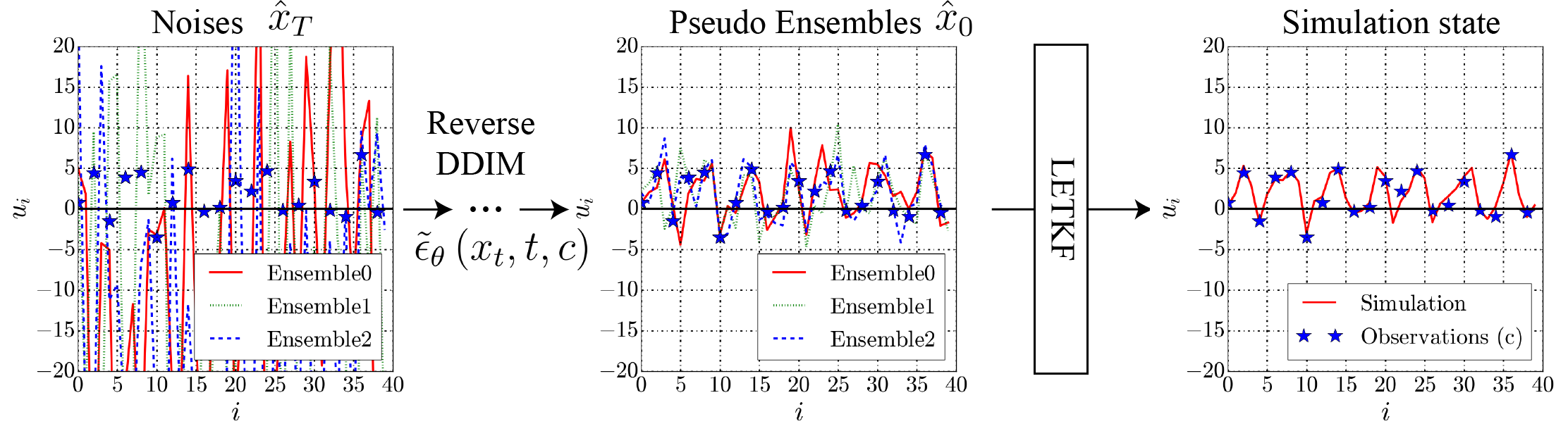
Figure 1: Proposed DA method with 3 pseudo ensembles. Pseudo ensembles are generated by reverse DDIM from noises. We compute the analysis state vectors by applying LETKF to these ensembles. Then, we update the simulation state by the average of the ensemble mean and the current simulation state.

2.1 Lorenz96 model

We employ the Lorenz96 model Lorenz & Emanuel (1998) as a minimal chaotic system defined by

$$\frac{du_{i}}{dt}=\left(u_{i+1}-u_{i-2}\right)u_{i-1}-u_{i}+F,~{}\left(\forall{i}=1,\ldots,N\right)$$ (1)

where $F$ means the forcing parameter and subscript $i$ denotes the $i$th state variable. We employ the periodic boundary condition with $u_{-1}=u_{N-1}$, $u_{0}=u_{N}$ and $u_{N+1}=u_{1}$. This model shows chaotic behaviour with $F=8$, but shows periodic or more chaotic behaviours with $F=5$ and $F=11$ (see Figs. 2 (a) and 2 (c)).

In this work, we perform an observing system simulation experiment (OSSE) using the Lorenz96 model as for a proof of concept. We first conduct a raw simulation of Lorenz96 in eq. (1) which is regarded as “Nature” run. We then add a Gaussian noise ${\cal N}\left(0,e\right)$ to the simulation results of “Nature” run to get mock “Observation” data. In this work, we choose the observation error as $e=1$. Our primary task is to predict the “Nature” run from the mock “Observation” data.

2.2 Lorenz96 dataset

Instead of ensemble simulations, we generate pseudo ensembles using DDPM guided by sparse and noisy “Observation” data. As a training dataset for DDPM, we performed the 100 Lorenz96 simulations with 1000 timesteps. Each member of dataset contains a snapshot of 40 state variables and mock “Observation” data corresponding to them. For pre-processing, we normalize each channel to the range of $[0,1]$.

2.3 Conditional Diffusion Model

We employ the diffusion model with classifier-free guidance Ho & Salimans (2022). This model consists of forward and backward diffusion processes. The forward process uses a Markov chain where the Gaussian noise is gradually added to the original data $x_{0}$. For the length $T$ diffusion steps, the latent variable $x_{t}$ at time $t\in\left[1,\ldots,T\right]$ is

$$x_{t}=\sqrt{\overline{\alpha}_{t}}x_{0}+\sqrt{1-\overline{\alpha}_{t}}\epsilon_{t},$$ (2)

where $\epsilon_{t}\sim{\cal N}\left(0,\mathbf{I}\right)$, $\overline{\alpha}_{t}=\prod_{s=1}^{t}\left(1-\beta_{s}\right)$ and $\beta_{t}$ is a fixed variance schedule. The backward process or sampling process in turn generates a clean data from noises by

$$x_{t-1}=\frac{1}{\sqrt{1-\beta_{t}}}\left(x_{t}-\frac{\beta_{t}}{\sqrt{1-\alpha_{t}}}\tilde{\epsilon}_{\theta}\left(x_{t},t,c\right)\right)+\sigma_{t}\epsilon_{t},$$ (3)

where $c$ is the conditioning information and $\sigma_{t}$ is the variance of the noise. $\tilde{\epsilon}_{\theta}$ is the linear combination of the conditional and unconditional score estimates as

$$\tilde{\epsilon}_{\theta}\left(x_{t},t,c\right)=\left(1+w\right)\epsilon_{\theta}\left(x_{t},c\right)-w\epsilon_{\theta}\left(x_{t},\emptyset\right),$$ (4)

with the conditioning strength $w$. We set $w=3$ for sampling. We employ the 1D U-Net Ronneberger et al. (2015) based model to approximate $\epsilon_{\theta}\left(x_{t},c\right)$. In the training, we use a single model to parameterize the conditional $\epsilon_{\theta}\left(x_{t},c\right)$ and unconditional $\epsilon_{\theta}\left(x_{t},\emptyset\right)$ scores by randomly discarding the conditioning during training Ho & Salimans (2022). For each observation interval, we train a separate diffusion model with $T=1000$. The noisy and sparse “Observations” $c$ are given in the same shape as the original data with zero filling wherein “Observations” are unavailable. It should be noted that the unconditional labels are given by learnable parameters which are different from zeros in observations. To accelerate the sampling procedure, we use the Denoising Diffusion Implicit Model (DDIM) Song et al. (2020) with $T=100$, rather than directly using DDPM. We train the model for $100000$ steps with the batch size of 16. We use the Adam optimizer Kingma & Ba (2015) with the learning rate $0.001$.

2.4 DA method

Figure 1 illustrates the DA process using DDPM. In each DA step, we generate pseudo ensembles with pre-trained diffusion models from noises guided by “Observation” data. We apply LETKF to these pseudo ensembles to compute analysis state vectors. We consider the ensemble mean of state vectors as the best estimate. The average of the ensemble mean and the simulation state vector is considered as the data-assimilated simulation state. In EnKF, the numerical model is used to forecast the next states and the observations are used to alter the current states of the model. This way, the numerical models can start prediction from better model states. In the proposed method, the numerical model is used to generate the dataset and DDPM is trained to reproduce its data distribution guided by the observations. The generated ensembles are thus close to the observations. In our method, the information from past observation is carried through the data-assimilated simulation state vector which is the average of the ensemble and the simulation state vector.

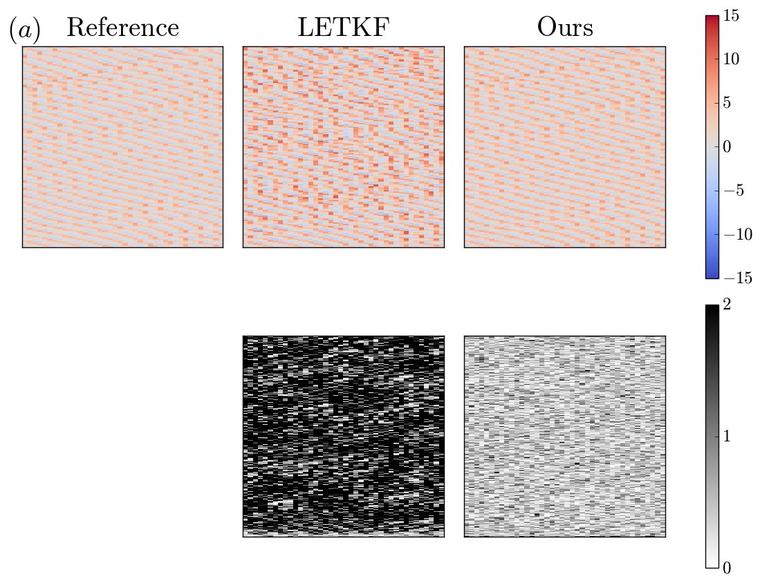
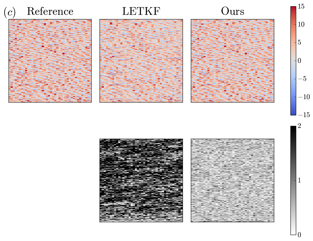
Figure 2: Hovmöller diagrams and errors with (a) $F=5$, (b) $F=8$, and (c) $F=11$ cases. The upper row includes the Hovmöller diagrams of reference, LETKF and our method, respectively. The bottom row includes the absolute errors between reference and DA simulations with LETKF and our method.

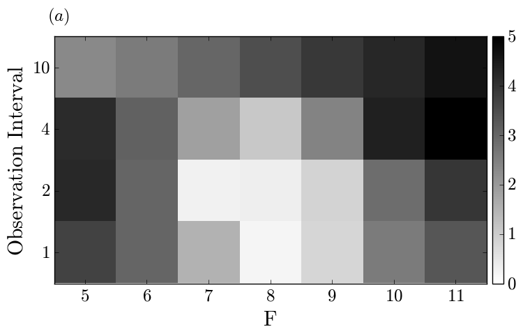
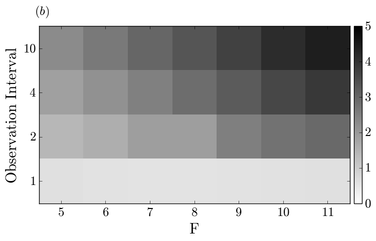
Figure 3: The dependency of RMSE with respect to the model bias and the observation interval. (a) LETKF and (b) our method.

3 Experiment

In this section, we compare the performance of DA with LETKF and ours. We trained DDPM guided by sparse and noisy “Observation” data for the simulations with $F=8$. For LETKF, we perform 32 ensemble simulations. For our method, we perform a non-ensemble simulation and generate 32 ensembles from observation data. We compute the analysis state vectors by applying LETKF to these ensembles. Then, we update the simulation state by the average of the ensemble mean and the current simulation state. DA is applied at each time step. We perform simulations with $F=8$ and assimilate the simulation states with the “Observation” data obtained from different “Nature” runs using multiple $F$ values with $F\in\left[5-11\right]$. Although we expect a performance gain with the proposed method for more complicated numerical models, DDIM sampling to generate ensembles is more costly than ensemble simulations of Lorenz96 system. The performance aspect of the proposed method will be discussed with more complicated applications in a separate publication.

Figure 2 shows the Hovmöller diagrams of “Nature” runs and simulations with DA for the observation interval of 1 (40 observation points). As found in Fig. 2 (b), when the model is not biased (the $F$ value is the same or similar for simulation and observation), LETKF displays better accuracy than ours. For $F=5$ and $F=11$, our method exhibits better accuracy than LETKF. In these biased cases, LETKF fails due to the filter divergence issue Ng et al. (2011). The filter becomes overconfident around an incorrect state and thus the subsequent observations are ignored. It happens when the variance of ensembles is too small. The estimate cannot be moved back toward the true state. In contrast, our model always tracks the observations and the variance of ensembles is kept due to the properties of DDPM. Accordingly, our model stays closer to “Observation” data and filter divergence can be suppressed.

We investigate the impact of model biases (imperfectness of model) and observation intervals (imperfectness of observation) on the performance of DA methods. Figure 3 shows the time averaged root mean square errors (RMSEs) between reference and DA simulations with LETKF and our method. As shown in Fig. 3 (a), LETKF gives good prediction up to observation interval of 4 if “Nature” runs are made with $F\in\left[7-9\right]$. Other than these cases, our model exhibits better performance as shown in Fig. 3 (b). Our model outperforms LETKF when the incompleteness of models and observations are large. This is a preferable behaviour for DA considering that model biases are basically inevitable in real life.

4 Summary

In this work, we have proposed a DA method that relies on pseudo ensembles generated by DDPM. It has turned out that the proposed DA method is robust against the imperfectness of models (model biases) and observations (noises and sparsity). By using DDPM guided by noisy and sparse observations, we can generate divergent pseudo ensembles close to observation data. We can update the simulation result in the framework of LETKF using these ensembles. We compare the prediction accuracy of proposed DA method against LETKF with ensemble simulations. The proposed method outperforms LETKF particularly when the model is biased.

Accessibility

For better color accessibility, we use both multiple colors and line types in Figure 1. In order to display the error levels in Figs. 2 and 3, we avoid using color and show the intensity in gray scale. For all figures, we have enlarged the captions.

Software and Data

The source codes and dataset are available in the Github repository Asahi (2023).

Broader impact

We have demonstrated the performance of NN based DA method in a simple 1D chaotic system. The proposed method is robust against the imperfectness of models (model biases) and observations (noises and sparsity). In principle, this method is applicable to 2D or even 3D simulations, which are used in various scientific domains.

Appendix

Here, we describe the details of Local ensemble transform Kalman Filter (LETKF) Hunt et al. (2007) in the context of ensemble Data assimilation (DA). In general, DA deals with a dynamical system defined by

$$\mathbf{x}^{f}_{j} = {\cal M}_{j}\left(\mathbf{x}^{a}_{j-1}\right),$$ (5)

$$\mathbf{y}_{j}^{o} = {\cal H}_{j}\left(\mathbf{x}^{t}_{j}\right)+\mathbf{\epsilon}_{j},~{}\mathbf{\epsilon}_{j}\sim{\cal N}\left(0,\mathbf{R}_{j}\right),$$ (6)

$$\mathbf{x}^{a}_{j} = \mathbf{x}^{t}_{j}+\mathbf{\eta}_{j},~{}\mathbf{\eta}_{j}\sim{\cal N}\left(0,\mathbf{P}_{j}^{a}\right)$$ (7)

where $\mathbf{x}^{f}_{j}$ denotes the forecast variables, $\mathbf{x}^{a}_{j-1}$ denotes the analysis variables, $\mathbf{x}^{t}_{j}$ represents the “true” state, and $\mathbf{y}^{o}_{j}$ is a vector of observed values. ${\cal M}_{j}$ represents the nonlinear dynamical model for time evolution from time $t_{j-1}$ to time $t_{j}$. ${\cal H}_{j}$ is the observation operator which projects the forecast variables into the observation space with the observation error $\mathbf{\epsilon}_{j}$. The analysis variables $\mathbf{x}^{a}_{j}$ are assumed to be apart from the “true” state $\mathbf{x}^{t}_{j}$ with the stochastic error $\mathbf{\eta}_{j}$. These errors are respectively assumed to be non-biased (zero mean) Gaussian distributions with the covariance matrices $\mathbf{R}_{j}$ and $\mathbf{P}_{j}^{a}$.

In DA, the model is used to forecast variables at the next time step from the current analysis variables (forecast step). Then, the current observation data are used to update the prior forecast variables to current state estimates which maximize the Bayesian likelihood (analysis step).

LETKF is based on Kalman Filter (KF) which estimates the state vector $\mathbf{x}^{a}_{j}$ at time $t_{j}$ with the following linearized equations.

$$\mathbf{x}^{a}_{j} = \mathbf{x}^{f}_{j}+\mathbf{K}_{j}\left(\mathbf{y}_{j}^{o}-\mathbf{H}_{j}\mathbf{x}_{j}^{f}\right),$$ (8)

$$\mathbf{K}_{j} = \mathbf{P}_{j}^{f}\mathbf{H}_{j}^{\top}\left(\mathbf{H}_{j}\mathbf{P}_{j}^{f}\mathbf{H}_{j}^{\top}+\mathbf{R}_{j}\right)^{-1},$$ (9)

$$\mathbf{P}_{j}^{a} = \left(\mathbf{I}-\mathbf{K}_{j}\mathbf{H}_{j}\right)\mathbf{P}_{j}^{f},$$ (10)

where the superscripts $f$ and $a$ respectively denote the forecast and analysis, $\mathbf{y}_{j}^{o}$ is the observation vector, $\mathbf{I}$ is the identity matrix, $\mathbf{H}_{j}$ is the observation matrix which projects the state vector $\mathbf{x}_{j}^{f}$ into the observation space, and $\mathbf{K}_{j}$ is a matrix called the Kalman gain. Here, matrix $\mathbf{H}_{j}$ is the linearization of the observation operator ${\cal H}_{j}$. The time evolution operator is also linearlized to give $\mathbf{x}^{f}_{j}=\mathbf{M}_{j}\mathbf{x}^{a}_{j-1}$. The Kalman gain $\mathbf{K}_{j}$ defined by eq. (9) gives the most likely state $\mathbf{x}^{a}_{j}$ given the observations up to time $t_{j}$ in a least square sense. For simplicity, we hereinafter omit the subscript $j$ representing time.

Unfortunately, when the number of model variables $m$ is huge (this is often the case for real-world models such as a global weather model), computing the covariance matrix $\mathbf{P}$ is a formidable task involving the $m\times m$ matrix operations. Instead, we use ensembles of model states to approximate $\mathbf{P}$.

In LETKF, the analysis vector $\mathbf{x}^{a}$ of the $m$-th ensemble is computed by

$$\mathbf{x}_{m}^{a}=\overline{\mathbf{x}}^{f}+\delta\mathbf{X}^{f}\left(\overline{\mathbf{w}}^{a}+\delta\mathbf{W}_{m}^{a}\right),$$ (11)

where $\overline{\mathbf{w}}^{a}$ and $\delta\mathbf{W}_{m}^{a}$ are the mean of the transformed vector and the $m$-th column of the perturbation of the transformed vector. These are calculated by

$$\overline{\mathbf{w}}^{a} = \tilde{\mathbf{P}}^{a}\delta\mathbf{Y}^{f\top}\mathbf{R}^{-1}\left(\mathbf{y}^{o}-\overline{\mathbf{y}}^{f}\right),$$ (12)

$$\delta\mathbf{W}^{a} = \left[\left(N_{e}-1\right)\tilde{\mathbf{P}}^{a}\right]^{1/2},$$ (13)

where $N_{e}$ is the number of ensembles. $\mathbf{y}^{f}\left(=\mathbf{H}\mathbf{x}^{f}\right)$ is the observation vector computed from the model state $\mathbf{x}^{f}$. The inflation coefficient $\beta$ is introduced to mitigate the so-called filter divergence problem, resulting from the small error covariance. The matrix $\mathbf{R}$ represents the observation error covariance, on which localization is applied to suppress the spurious long-distance correlation. The covariance matrix $\tilde{\mathbf{P}}^{a}$ is defined as

$$\tilde{\mathbf{P}}^{a}=\left[\frac{\left(N_{e}-1\right)}{\beta}\mathbf{I}+\delta\mathbf{Y}^{f\top}\mathbf{R}^{-1}\delta\mathbf{Y}^{f}\right]^{-1}\equiv\mathbf{Q}^{-1}.$$ (14)

The ensemble mean $\overline{\mathbf{x}}^{f}$ and $\overline{\mathbf{y}}^{f}$, and perturbation matrices $\delta\mathbf{X}^{f}$ and $\delta\mathbf{Y}^{f}$ are defined by

$$\overline{\mathbf{x}}^{f} = \frac{1}{N_{e}}\sum_{m=0}^{N_{e}-1}\mathbf{x}_{m}^{f},$$ (15)

$$\delta\mathbf{X}^{f} = \left[\mathbf{x}_{0}^{f}-\overline{\mathbf{x}}^{f},\mathbf{x}_{1}^{f}-\overline{\mathbf{x}}^{f},\ldots,\mathbf{x}_{N_{e}-1}^{f}-\overline{\mathbf{x}}^{f}\right],$$ (16)

$$\overline{\mathbf{y}}^{f} = \frac{1}{N_{e}}\sum_{m=0}^{N_{e}-1}\mathbf{y}_{m}^{f},$$ (17)

$$\delta\mathbf{Y}^{f} = \left[\mathbf{y}_{0}^{f}-\overline{\mathbf{y}}^{f},\mathbf{y}_{1}^{f}-\overline{\mathbf{y}}^{f},\ldots,\mathbf{y}_{N_{e}-1}^{f}-\overline{\mathbf{y}}^{f}\right].$$ (18)

$\tilde{\mathbf{P}}^{a}$ and $\left[\tilde{\mathbf{P}}^{a}\right]^{1/2}$ can be efficiently computed by the Eigen Value Decomposition (EVD) of $\mathbf{Q}$. In LETKF, we apply the localization on $\mathbf{R}$ as $\mathbf{R}_{\rm loc}^{-1}=\mathbf{G}\circ\mathbf{R}^{-1}$, which decompose the analysis procedure into a local problem on each grid point. As the local problem is independent on each grid point, LETKF is highly parallelizable and thus suitable for many recent parallel architectures such as GPUs. In the present work, the localization function is given by the Gaspari-Cohn function Gaspari & Cohn (1999), in which the cutoff distance is chosen as $d=2\left(p-1\right)\Delta x$ based on the distance between observation points $p\Delta x$, where $p$ and $\Delta x$ denote the observation interval and grid width, respectively.

References

- Asahi (2023) Asahi, Y. Generative-EnKF. https://github.com/yasahi-hpc/Generative-EnKF, 2023.
- Bannister (2017) Bannister, R. N. A review of operational methods of variational and ensemble-variational data assimilation. Quarterly Journal of the Royal Meteorological Society, 143(703):607–633, 2017. doi: https://doi.org/10.1002/qj.2982. URL https://rmets.onlinelibrary.wiley.com/doi/abs/10.1002/qj.2982.
- Barthélémy et al. (2022) Barthélémy, S., Brajard, J., Bertino, L., and Counillon, F. Super-resolution data assimilation. Ocean Dynamics, 72(8):661–678, Aug 2022. ISSN 1616-7228. doi: 10.1007/s10236-022-01523-x. URL https://doi.org/10.1007/s10236-022-01523-x.
- Chattopadhyay et al. (2023) Chattopadhyay, A., Nabizadeh, E., Bach, E., and Hassanzadeh, P. Deep learning-enhanced ensemble-based data assimilation for high-dimensional nonlinear dynamical systems. Journal of Computational Physics, 477:111918, 2023. ISSN 0021-9991. doi: https://doi.org/10.1016/j.jcp.2023.111918. URL https://www.sciencedirect.com/science/article/pii/S002199912300013X.
- Evensen (1994) Evensen, G. Sequential data assimilation with a nonlinear quasi-geostrophic model using Monte Carlo methods to forecast error statistics. Journal of Geophysical Research: Oceans, 99(C5):10143–10162, 1994. doi: https://doi.org/10.1029/94JC00572. URL https://agupubs.onlinelibrary.wiley.com/doi/abs/10.1029/94JC00572.
- Evensen (2003) Evensen, G. The Ensemble Kalman Filter: theoretical formulation and practical implementation. Ocean Dynamics, 53(4):343–367, Nov 2003. ISSN 1616-7228. doi: 10.1007/s10236-003-0036-9. URL https://doi.org/10.1007/s10236-003-0036-9.
- Gaspari & Cohn (1999) Gaspari, G. and Cohn, S. E. Construction of correlation functions in two and three dimensions. Quarterly Journal of the Royal Meteorological Society, 125(554):723–757, 1999. doi: https://doi.org/10.1002/qj.49712555417. URL https://rmets.onlinelibrary.wiley.com/doi/abs/10.1002/qj.49712555417.
- Grooms (2021) Grooms, I. Analog ensemble data assimilation and a method for constructing analogs with variational autoencoders. Quarterly Journal of the Royal Meteorological Society, 147(734):139–149, 2021. doi: https://doi.org/10.1002/qj.3910. URL https://rmets.onlinelibrary.wiley.com/doi/abs/10.1002/qj.3910.
- Ho & Salimans (2022) Ho, J. and Salimans, T. Classifier-free diffusion guidance. arXiv preprint arXiv:2207.12598, 2022.
- Ho et al. (2020) Ho, J., Jain, A., and Abbeel, P. Denoising diffusion probabilistic models. Advances in Neural Information Processing Systems, 33:6840–6851, 2020.
- Hunt et al. (2007) Hunt, B. R., Kostelich, E. J., and Szunyogh, I. Efficient data assimilation for spatiotemporal chaos: A local ensemble transform Kalman filter. Physica D: Nonlinear Phenomena, 230(1):112–126, 2007. ISSN 0167-2789. doi: https://doi.org/10.1016/j.physd.2006.11.008. URL https://www.sciencedirect.com/science/article/pii/S0167278906004647. Data Assimilation.
- Kingma & Ba (2015) Kingma, D. P. and Ba, J. Adam: A method for stochastic optimization. In ICLR (Poster), 2015. URL http://arxiv.org/abs/1412.6980.
- Liu et al. (2022) Liu, C., Fu, R., Xiao, D., Stefanescu, R., Sharma, P., Zhu, C., Sun, S., and Wang, C. EnKF data-driven reduced order assimilation system. Engineering Analysis with Boundary Elements, 139:46–55, 2022. ISSN 0955-7997. doi: https://doi.org/10.1016/j.enganabound.2022.02.016. URL https://www.sciencedirect.com/science/article/pii/S0955799722000510.
- Lorenz & Emanuel (1998) Lorenz, E. N. and Emanuel, K. A. Optimal Sites for Supplementary Weather Observations: Simulation with a Small Model. Journal of the Atmospheric Sciences, 55(3):399 – 414, 1998. doi: https://doi.org/10.1175/1520-0469(1998)055¡0399:OSFSWO¿2.0.CO;2. URL https://journals.ametsoc.org/view/journals/atsc/55/3/1520-0469_1998_055_0399_osfswo_2.0.co_2.xml.
- Miyoshi et al. (2014) Miyoshi, T., Kondo, K., and Imamura, T. The 10,240-member ensemble Kalman filtering with an intermediate AGCM. Geophysical Research Letters, 41(14):5264–5271, 2014. doi: https://doi.org/10.1002/2014GL060863. URL https://agupubs.onlinelibrary.wiley.com/doi/abs/10.1002/2014GL060863.
- Ng et al. (2011) Ng, G. H. C., McLaughlin, D., Entekhabi, D., and Ahanin, A. The role of model dynamics in ensemble Kalman filter performance for chaotic systems. Tellus, Series A: Dynamic Meteorology and Oceanography, 63(5):958–977, 2011. ISSN 02806495. doi: 10.1111/j.1600-0870.2011.00539.x.
- Ouala et al. (2018) Ouala, S., Fablet, R., Herzet, C., Chapron, B., Pascual, A., Collard, F., and Gaultier, L. Neural Network Based Kalman Filters for the Spatio-Temporal Interpolation of Satellite-Derived Sea Surface Temperature. Remote Sensing, 10(12), 2018. ISSN 2072-4292. doi: 10.3390/rs10121864. URL https://www.mdpi.com/2072-4292/10/12/1864.
- Peyron et al. (2021) Peyron, M., Fillion, A., Gürol, S., Marchais, V., Gratton, S., Boudier, P., and Goret, G. Latent space data assimilation by using deep learning. Quarterly Journal of the Royal Meteorological Society, 147(740):3759–3777, 2021. doi: https://doi.org/10.1002/qj.4153. URL https://rmets.onlinelibrary.wiley.com/doi/abs/10.1002/qj.4153.
- Ronneberger et al. (2015) Ronneberger, O., P.Fischer, and Brox, T. U-Net: Convolutional Networks for Biomedical Image Segmentation. In Medical Image Computing and Computer-Assisted Intervention (MICCAI), volume 9351 of LNCS, pp. 234–241. Springer, 2015. URL http://lmb.informatik.uni-freiburg.de/Publications/2015/RFB15a. (available on arXiv:1505.04597 [cs.CV]).
- Sacher & Bartello (2008) Sacher, W. and Bartello, P. Sampling Errors in Ensemble Kalman Filtering. Part I: Theory. Monthly Weather Review, 136(8):3035 – 3049, 2008. doi: https://doi.org/10.1175/2007MWR2323.1. URL https://journals.ametsoc.org/view/journals/mwre/136/8/2007mwr2323.1.xml.
- Sacher & Bartello (2009) Sacher, W. and Bartello, P. Sampling Errors in Ensemble Kalman Filtering. Part II: Application to a Barotropic Model. Monthly Weather Review, 137(5):1640 – 1654, 2009. doi: https://doi.org/10.1175/2008MWR2685.1. URL https://journals.ametsoc.org/view/journals/mwre/137/5/2008mwr2685.1.xml.
- Song et al. (2020) Song, J., Meng, C., and Ermon, S. Denoising diffusion implicit models. arXiv preprint arXiv:2010.02502, 2020.
- Tomizawa & Sawada (2021) Tomizawa, F. and Sawada, Y. Combining ensemble Kalman filter and reservoir computing to predict spatiotemporal chaotic systems from imperfect observations and models. Geoscientific Model Development, 14(9):5623–5635, 2021. doi: 10.5194/gmd-14-5623-2021. URL https://gmd.copernicus.org/articles/14/5623/2021/.
- Tsuyuki & Tamura (2022) Tsuyuki, T. and Tamura, R. Nonlinear Data Assimilation by Deep Learning Embedded in an Ensemble Kalman Filter. Journal of the Meteorological Society of Japan, advpub:2022–027, 2022. doi: 10.2151/jmsj.2022-027.
- Yang & Grooms (2021) Yang, L. M. and Grooms, I. Machine learning techniques to construct patched analog ensembles for data assimilation. Journal of Computational Physics, 443:110532, 2021. ISSN 0021-9991. doi: https://doi.org/10.1016/j.jcp.2021.110532. URL https://www.sciencedirect.com/science/article/pii/S0021999121004277.
- Yasuda & Onishi (2022) Yasuda, Y. and Onishi, R. Spatio-Temporal Super-Resolution Data Assimilation (SRDA) Utilizing Deep Neural Networks with Domain Generalization Technique Toward Four-Dimensional SRDA. arXiv preprint arXiv:2212.03656, 2022.