Hypothesis testing for medical imaging analysis via the smooth Euler characteristic transform

Abstract

Shape-valued data are of interest in applied sciences, particularly in medical imaging. In this paper, inspired by a specific medical imaging example, we introduce a hypothesis testing method via the smooth Euler characteristic transform to detect significant differences among collections of shapes. Our proposed method has a solid mathematical foundation and is computationally efficient. Through simulation studies, we illustrate the performance of our proposed method. We apply our method to images of lung cancer tumors from the National Lung Screening Trial database, comparing its performance to a state-of-the-art machine learning model.

1 Introduction

Medical imaging plays a pivotal role in modern healthcare, offering invaluable insights into diagnosing, treating, and monitoring various medical conditions. Among these, images of tumors hold particularly crucial importance. These images, generated through advanced techniques such as computed tomography (CT), magnetic resonance imaging (MRI), and positron emission tomography (PET), provide clinicians with a visual window into the internal structures of the human body, enabling early detection and accurate characterization of tumors.

Statistical inference in medical imaging (Bankman, 2008) holds immense importance as it provides the means to draw meaningful conclusions from image data. It validates findings obtained by medical professionals, ensuring they are not the result of chance.

Figure 1: The first two rows represent malignant nodules and the last two rows represent benign nodules.

1.1 Motivating Questions

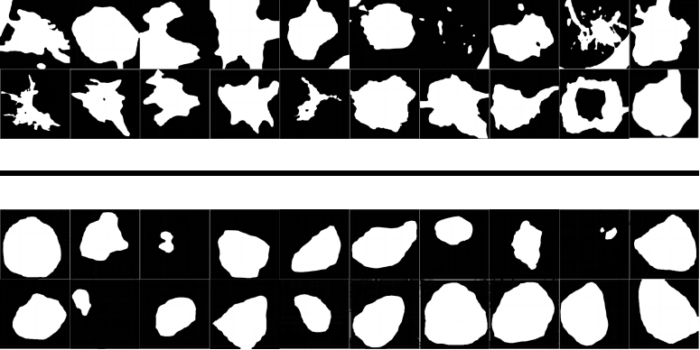
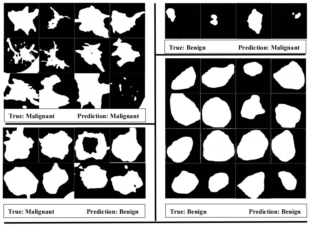
By analyzing CT imaging, medical professionals can often distinguish between malignant and benign tumors. Malignant tumors tend to exhibit certain features on CT images that can help differentiate them from benign tumors. These features may include irregular shapes and poorly defined edges. For example, the (binary segmented) CT scans presented in Figure 1 are from the National Lung Screening Trial database (Maldonado et al., 2021). Each of the scans has been labeled by medical professionals as either malignant or benign. One may ask: “Do the shapes of malignant tumors differ significantly from those of benign tumors?” A subsequent question is: “How much statistical power do we have in distinguishing the malignant and benign groups?” These questions motivate our study in this paper.

Many statistical inference methods can be used to address the motivating questions, but efficacy can be compromised by the imposition of stringent model assumptions, especially parametric ones. For example, logistic regression estimates the probability of malignancy using CT features. However, the method’s presumption of linearity and independence may not universally apply. Bayesian methods generally depend on and are sensitive to prior distributions.

To address the motivating questions and overcome the referred issues the statistical inference methods suffer from, in this paper, we will propose a distribution-free method via topological data analysis (TDA) (Carlsson, 2009).

1.2 Overview of Topological Data Analysis and Its Applications

TDA is a rapidly growing field that applies algebraic and computational topology to analyze complex data sets (Hatcher, 2002, Edelsbrunner and Harer, 2022, Wasserman, 2018). One of the central techniques in TDA is persistence homology (Edelsbrunner et al., 2000). The application of persistence homology has proven to be highly effective in a wide range of applications: in bioimage informatics, persistence homology has been used to extract topological information from the single molecule localization microscopy data (Pike et al., 2019); in phylogenetics, persistence homology has been used to analyze the physical features that best describe the variation between mandibular molars from four different suborders of primates (Wang et al., 2021, Meng et al., 2022); persistence homology has also been applied to radio-genomics (Crawford et al., 2020) and morphology (Turner et al., 2014, Marsh et al., 2022).

Based on persistent homology, Crawford et al. (2020) proposed the smooth Euler characteristic transform (SECT) to analyze glioblastoma multiforme. The mathematical foundations of SECT were developed from the Euler calculus viewpoint by Ghrist et al. (2018) and from the random fields viewpoint by Meng et al. (2022). Specifically, Ghrist et al. (2018) showed that SECT does not lose any information on shapes when it transforms shape-valued data into functional data; Meng et al. (2022) showed that SECT could be viewed as a random variable taking values in a separable Banach space.

Shape-valued data are of interest in many applied sciences, e.g., the tumors discussed in the motivating questions in Section 1.1. The analysis of shape-valued data is still underdeveloped, while functional data analysis has been well developed (Wang et al., 2016). Using persistent homology, we may transform shape-valued data into functional data, which allows us to implement many tools in functional analysis (Brezis, 2011) and functional data analysis.

1.3 Major Contributions and Paper Organization

In this paper, we apply the SECT to transform shape-valued data into functional data. Then, we apply the null hypothesis significance testing (NHST, Robinson and Turner (2017)) to the functional data. This approach was motivated by Meng et al. (2022). The combination of SECT and NHST provides us with an effective approach to inferring the differences between two collections of shapes (e.g., the malignant and benign collections of tumors presented in Figure 1).

This paper is organized as follows. In Section 2, we provide an overview of the existing background theory for SECT and our proposed hypothesis testing algorithm. We then present proof-of-concept simulation studies in Section 3 to show the performance of our proposed algorithm. In Section 4, we apply our algorithm to the images of lung cancer tumors from the National Lung Screening Trial database. Therein, we compare the performance of our algorithm with a state-of-the-art machine learning approach. A conclusion of this paper is given in Section 5.

2 Theory and Method

In this section, we first provide a brief description of SECT (Section 2.1). Then, we propose our hypothesis testing approach (Section 2.2).

2.1 Smooth Euler Characteristic Transform

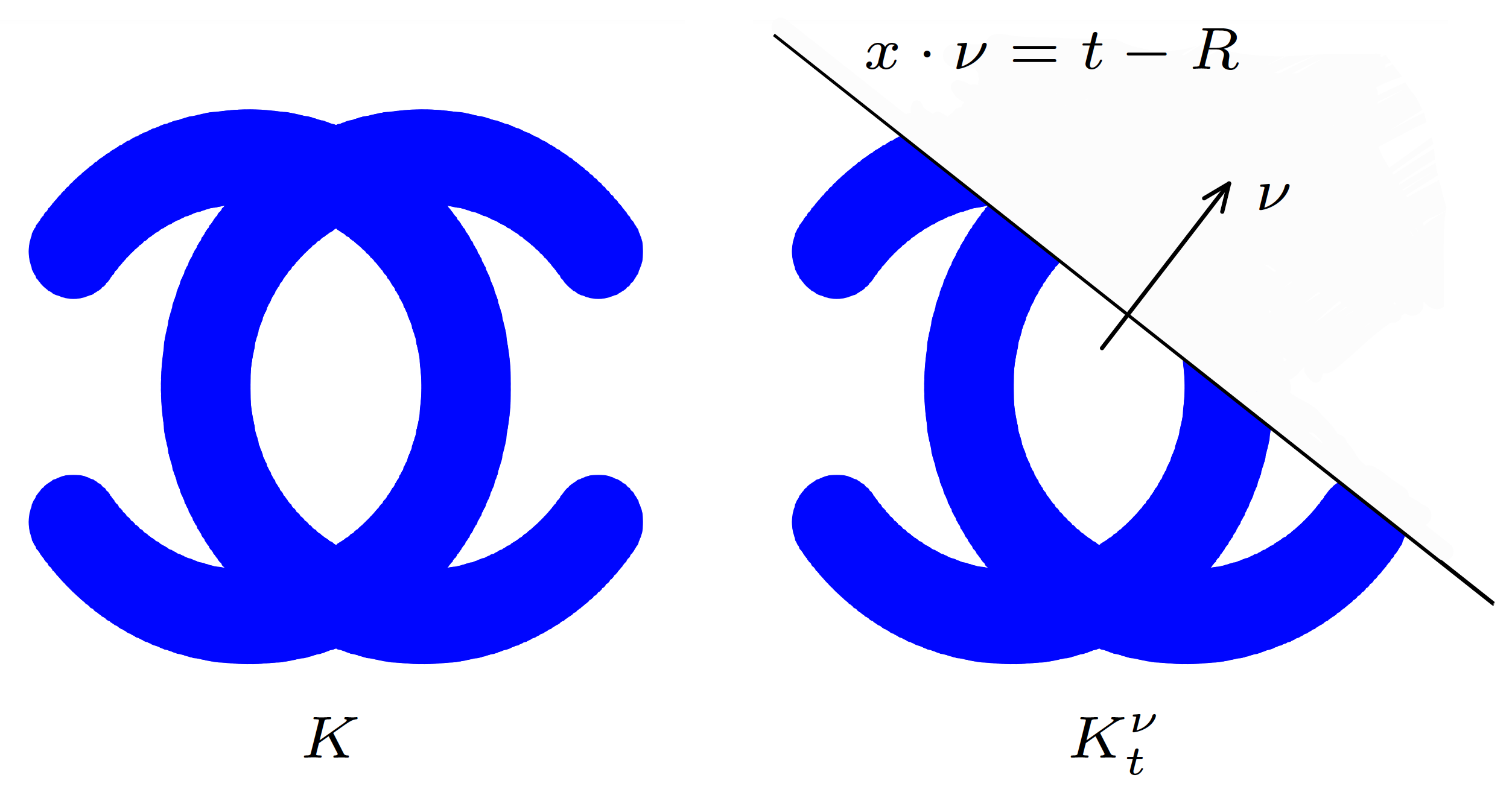
Let $K$ denote a compact subset of $d$-dimensional space $\mathbb{R}^{d}$ (referred to as a “shape” hereafter), e.g., the tumors in Figure 1 and the shape in Figure 2. We assume the shapes of interest are bounded by a ball with a finite radius, i.e., $K\subseteq B(0,R)$, where $B(0,R)=\{x\in\mathbb{R}^{d}:\|x\|<R\}$ denotes the open ball centered at the origin with some radius $R>0$. For each direction represented by a unit vector $\nu\in\mathbb{S}^{d-1}=\{x\in\mathbb{R}^{d}\,:\,\|x\|=1\}$ and scalar $t\in[0,2R]$, we define the following subset of $K$

$$K_{t}^{\nu}\overset{\operatorname{def}}{=}\left\{x\in K:x\cdot\nu\leq t-R\right\}.$$ (2.1)

One example illustrating the $K_{t}^{\nu}$ defined in Eq. (2.1) is presented in Figure 2. For succinctness, we denote $T\overset{\operatorname{def}}{=}2R$ hereafter.

Figure 2: The shape in the left panel is denoted by $K$. For each direction $\nu\in\mathbb{S}^{d-1}$ and scalar $t\in[0,2R]$, the straight line (or hyperplane for high dimensional scenarios) represented by linear equation $x\cdot\nu=t-R$ is associated with them. Then, $K_{t}^{\nu}$ is the collection of points in the $K$ that are below this straight line.

Let $\chi(K_{t}^{\nu})$ denote the Euler characteristic of $K_{t}^{\nu}$. If the subset $K_{t}^{\nu}$ is a discrete polygon mesh in computer graphics, we have $\chi(K_{t}^{\nu})=\#V-\#E+\#F$, where $\#V$, $\#E$, and $\#F$ are the numbers of vertices, edges, and faces of $K_{t}^{\nu}$, respectively. Take a triangle (including its face enclosed by its three edges) as an example; the numbers of vertices, edges, and faces of a triangle are 3, 3, and 1, respectively. Therefore, the Euler characteristic of a triangle is 1. When $K_{t}^{\nu}$ is not a polygon mesh, the general definition of its Euler characteristic is available in Hatcher (2002). Efficient algorithms and examples for computing Euler characteristics in statistical applications are available in the literature (e.g., Crawford et al. (2020) and Wang et al. (2021)). The SECT of shape $K$, denoted as $\operatorname{SECT}(K)$, is a function defined on the Cartesian product space $\mathbb{S}^{d-1}\times[0,T]$. Specifically, $\operatorname{SECT}(K)$ is defined by the following

$$\operatorname{SECT}:\ \ K\mapsto\operatorname{SECT}(K)=\left\{\operatorname{SECT}(K)(\nu,t)\right\}_{(\nu,t)\in\mathbb{S}^{d-1}\times[0,T]},$$

$$\text{where }\ \ \ \operatorname{SECT}(K)(\nu;t)\overset{\operatorname{def}}{=}\int_{0}^{t}\chi(K_{\tau}^{\nu})\,d\tau-\frac{t}{T}\int_{0}^{T}\chi(K_{\tau}^{\nu})\,d\tau.$$

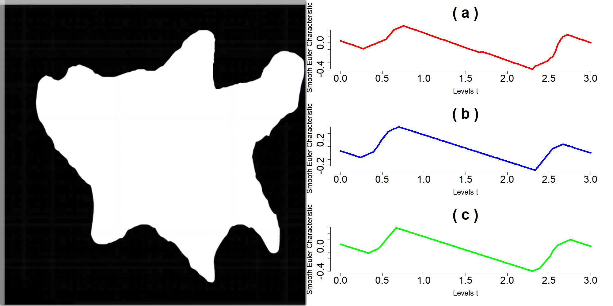
Visualizations of the $\operatorname{SECT}(K)(\nu;t)$ defined above are presented in Figures 4 and 5. Under some topological conditions, Ghrist et al. (2018) showed that the shape-to-function transform $K\mapsto\operatorname{SECT}(K)$ is invertible, i.e., $\operatorname{SECT}(K)$ contains all the information of shape $K$; in addition, if the shape $K$ is random, Meng et al. (2022) showed that $\operatorname{SECT}(K)$ is a random variable taking values in a separable Banach space.

Using the mathematical framework developed in Meng et al. (2022), one can easily show that $\operatorname{SECT}(K)$ belongs to $C(\mathbb{S}^{d-1};L^{2}(0,T))=$ the collection of all $L^{2}(0,T)$-valued continuous functions defined on sphere $\mathbb{S}^{d-1}$, where the function space $C(\mathbb{S}^{d-1};L^{2}(0,T))$ is a Banach space equipped with the norm

$$\|s\|_{C(\mathbb{S}^{d-1};L^{2}(0,T))}\overset{\operatorname{def}}{=}\sup_{\nu\in\mathbb{S}^{d-1}}\left\{\left(\int_{0}^{T}\left|s(\nu,t)\right|^{2}dt\right)^{1/2}\right\}.$$

Suppose two shapes $K^{(1)}$ and $K^{(2)}$ are given. As aforementioned, Ghrist et al. (2018) proved that all the information about each shape $K^{(i)}$ is contained by the corresponding $\operatorname{SECT}(K^{(i)})$. Hence, the dissimilarity between $K^{(1)}$ and $K^{(2)}$ can be measured by that between the two functions $\operatorname{SECT}(K^{(1)})(\nu,t)$ and $\operatorname{SECT}(K^{(2)})(\nu,t)$. Specifically, we measure the dissimilarity between two shapes by the following

$$\begin{aligned} \rho\left(K^{(1)},K^{(2)}\right)&\overset{\operatorname{def}}{=}\left\|\,\operatorname{SECT}(K^{(1)})-\operatorname{SECT}(K^{(2)})\,\right\|_{C(\mathbb{S}^{d-1};L^{2}(0,T))}\\ &=\sup_{\nu\in\mathbb{S}^{d-1}}\left\{\left(\int_{0}^{T}\left|\,\operatorname{SECT}(K^{(1)})(\nu;t)-\operatorname{SECT}(K^{(2)})(\nu;t)\,\right|^{2}dt\right)^{1/2}\right\}\end{aligned}$$ (2.2)

Our proposed hypothesis testing approach will be based on the dissimilarity function $\rho(\cdot,\cdot)$ defined in Eq. (2.2).

2.2 Randomization-style Null Hypothesis Significance Test via the Smooth Euler Characteristic Transform

The permutation test (Good, 2013) is a non-parametric statistical method that makes no distributional assumptions, making it versatile and applicable to a wide range of data sets. It is especially valuable for small sample sizes (e.g., the size of the malignant/benign tumor collection in Figure 1 is only 20) where traditional tests might lack power or their assumptions may not hold. Through rearranging observed data to assess the null hypothesis, the test offers an intuitive and exact approach, controlling the type I error rate effectively. In this subsection, we propose an algorithm for distinguishing two groups of shapes (e.g., the malignant and benign groups of tumors) via the permutation test.

Suppose there are two underlying shape-generating distributions, $\mathbb{P}^{(1)}$ and $\mathbb{P}^{(2)}$. Shape collections $\{K_{i}^{(1)}\}_{i=1}^{n_{1}}$ and $\{K_{i}^{(2)}\}_{i=1}^{n_{2}}$ are generated from $\mathbb{P}^{(1)}$ and $\mathbb{P}^{(2)}$, respectively, where the sample size $n_{1}$ is not necessarily equal to $n_{2}$ (i.e., unbalanced groups are allowed). We propose a SECT-based randomization-style null hypothesis significance test (NHST-SECT) to test the following hypotheses using collections $\{K_{i}^{(1)}\}_{i=1}^{n_{1}}$ and $\{K_{i}^{(2)}\}_{i=1}^{n_{2}}$

$$H_{0}:\ \ \mathbb{P}^{(1)}=\mathbb{P}^{(2)}\ \ \ vs.\ \ \ H_{1}:\ \ \mathbb{P}^{(1)}\neq\mathbb{P}^{(2)}.$$ (2.3)

Distinguishing the shape collections $\{K_{i}^{(1)}\}_{i=1}^{n_{1}}$ and $\{K_{i}^{(2)}\}_{i=1}^{n_{2}}$ is represented as rejecting the null hypothesis $H_{0}$ in Eq. (2.3). The randomization-style NHST-SECT is based on permutation test (Good, 2013) and the following loss functional

$$\begin{aligned} F\left(\{K_{i}^{(1)}\}_{i=1}^{n_{1}},\,\{K_{i}^{(2)}\}_{i=1}^{n_{2}}\right)\overset{\operatorname{def}}{=}\sum_{j=1}^{2}\frac{1}{2n_{j}(n_{j}-1)}\sum_{k,l=1}^{n_{j}}\rho\left(K_{k}^{(j)},\,K_{l}^{(j)}\right),\end{aligned}$$ (2.4)

where $\rho$ is the distance function defined in Eq. (2.2).

In applications, it is infeasible to calculate $\operatorname{SECT}(K_{i}^{(j)})(\nu,t)$ for all infinitely many directions $\nu\in\mathbb{S}^{d-1}$ and levels $t\in[0,T]$. Hence, we calculate the following discretized version in applications

$$\left\{\operatorname{SECT}(K_{i}^{(j)})(\nu_{p};t_{q}):p=1,\cdots,\Gamma\mbox{ and }q=1,\cdots,\Delta\right\}_{i=1}^{n_{j}},\ \ \text{ for }j\in\{1,2\},$$ (2.5)

where $\{\nu_{p}\}_{p=1}^{\Gamma}$ and $\{t_{q}\}_{q=1}^{\Delta}$ are prespecified. We choose $\{\nu_{p}\}_{p=1}^{\Gamma}$ uniformly from $\mathbb{S}^{d-1}$ and $\{t_{q}\}_{q=1}^{\Delta}$ uniformly from $[0,T]$, which is a standard approach in the literature, e.g., Crawford et al. (2020), and will be implemented in Section 4.1. The discretized SECT values in Eq. (2.5) are the input data for our statistical inference.

Given the discretized SECT in Eq. (2.5) as our data, we estimate the distance $\rho(K_{k}^{(j)},\,K_{l}^{(j)})$ by the following

$$\rho\left(K_{k}^{(j)},\,K_{l}^{(j)}\right)\approx\widehat{\rho}\left(K_{k}^{(j)},\,K_{l}^{(j)}\right)\overset{\operatorname{def}}{=}\sup_{p=1,\ldots,\Gamma}\left(\sum_{q=1}^{\Delta}\left|\operatorname{SECT}(K_{k}^{(j)})(\nu_{p};t_{q})-\operatorname{SECT}(K_{l}^{(j)})(\nu_{p};t_{q})\right|^{2}\right)^{1/2}.$$ (2.6)

Correspondingly, the value of the loss functional in Eq. (2.4) is approximated by the test statistic $\widehat{F}(\{K_{i}^{(1)}\}_{i=1}^{n_{1}},\{K_{i}^{(2)}\}_{i=1}^{n_{2}})$ defined as follows (the test statistic is derived by our input data in Eq. (2.4))

$$F\left(\{K_{i}^{(1)}\}_{i=1}^{n_{1}},\,\{K_{i}^{(2)}\}_{i=1}^{n_{2}}\right)\approx\widehat{F}\left(\{K_{i}^{(1)}\}_{i=1}^{n_{1}},\,\{K_{i}^{(2)}\}_{i=1}^{n_{2}}\right)\overset{\operatorname{def}}{=}\sum_{j=1}^{2}\frac{1}{2n_{j}(n_{j}-1)}\sum_{k,l=1}^{n_{j}}\widehat{\rho}\left(K_{k}^{(j)},\,K_{l}^{(j)}\right).$$ (2.7)

Based on the test statistic defined in Eq. (2.7), we apply Algorithm 1 to implement the NHST-SECT.

Algorithm 1 : Randomization-style NHST-SECT

1:Input: (i) Discretized SECT of two collection of shapes $\{\operatorname{SECT}(K_{i}^{(j)})(\nu_{p};t_{q}):p=1,\cdots,\Gamma\mbox{ and }q=1,\cdots,\Delta\}_{i=1}^{n_{j}}$ for $j\in\{1,2\}$; (ii) desired confidence level $1-\alpha$ with significance $\alpha\in(0,1)$; (iii) the number of permutations $\Pi$.

2:Output: Accept or Reject the null hypothesis $H_{0}$ in Eq. (2.3).

3:Apply Eq. (2.6) and Eq. (2.7) to the original input SECT data and compute the value of the loss $\mathfrak{S}_{0}\overset{\operatorname{def}}{=}\widehat{F}(\{K_{i}^{(1)}\}_{i=1}^{n},\,\{K_{i}^{(2)}\}_{i=1}^{n})$.

4:for all $k=1,\cdots,\Pi$,

5:Randomly permute the group labels $j\in\{1,2\}$ of the input SECT data.

6:Apply Eq. (2.6) and Eq. (2.7) to the permuted SECT data and compute the value of the loss $\mathfrak{S}_{k}\overset{\operatorname{def}}{=}\widehat{F}(\{K_{i}^{(1)}\}_{i=1}^{n},\,\{K_{i}^{(2)}\}_{i=1}^{n})$.

7:end for

8:Compute $k^{*}\overset{\operatorname{def}}{=}[\alpha\cdot\Pi]\overset{\operatorname{def}}{=}$ the largest integer smaller than $\alpha\cdot\Pi$.

9:Reject the null hypothesis $H_{0}$ if $\mathfrak{S}_{0}<\mathfrak{S}_{k^{*}}$ and report the output.

3 Experiments Using Simulations

This section presents simulation studies that demonstrate the performance of our randomization-style NHST-SECT framework presented in Algorithm 1. We also compare our proposed Algorithm 1 with the “ECT-based randomization-style null hypothesis significance test” presented in Algorithm 2 (see Appendix Appendix: ECT-based Randomization-style Null Hypothesis Significance Test), which was proposed in Robinson and Turner (2017) and Meng et al. (2022).

Our simulation studies focus on a family of distributions $\{\mathbb{P}^{(\varepsilon)}\}_{0\leq\varepsilon\leq 0.1}$, from which we generate a collection of i.i.d. shapes $\{K_{i}^{(\varepsilon)}\}_{i=1}^{n}$ for each $\varepsilon\in[0,0.1]$. For each $\varepsilon$, shapes generated from $\mathbb{P}^{(\varepsilon)}$ are presented as follows

$$K_{i}^{(\varepsilon)}= \left\{x\in\mathbb{R}^{2}\,\Bigg{|}\,\inf_{y\in S_{i}^{(\varepsilon)}}\|x-y\|\leq\frac{1}{5}\right\},\ \ \mbox{ where}$$ (3.1)

$$S_{i}^{(\varepsilon)}= \left\{\left(\frac{2}{5}+a_{1,i}\cdot\cos t,b_{1,i}\cdot\sin t\right)\,\Bigg{|}\,\frac{1-\varepsilon}{5}\pi\leq t\leq\frac{9+\varepsilon}{5}\pi\right\}\bigcup\left\{\left(-\frac{2}{5}+a_{2,i}\cdot\cos t,b_{2,i}\cdot\sin t\right)\,\Bigg{|}\,\frac{6\pi}{5}\leq t\leq\frac{14\pi}{5}\right\},$$

and $\{a_{1,i},a_{2,i},b_{1,i},b_{2,i}\}_{i=1}^{n}\overset{i.i.d.}{\sim}N(1,0.05^{2})$. The index $\varepsilon$ indicates the dissimilarity between distributions $\mathbb{P}^{(\varepsilon)}$ and $\mathbb{P}^{(0)}$. The varying values of $\varepsilon$ affect the shape generated from $\mathbb{P}^{(\varepsilon)}$. The shapes generated by different $\varepsilon$ across $[0,\,0.1]$ are presented in Figure 3. It is difficult to discern the differences between them by eye. But the TDA-based methods, especially our proposed Algorithm 1, can distinguish shapes corresponding to different $\varepsilon$ with high confidence. Notably, the images presented in Figure 3 resemble the image of a malignant lung cancer tumor (see the circle-like scan in the second row of Figure 1). We then test the following hypotheses using the scheme described in Algorithm 1

$$H_{0}:\,\mathbb{P}^{(0)}=\mathbb{P}^{(\varepsilon)}\ \ \ vs.\ \ \ H_{1}:\,\mathbb{P}^{(0)}\neq\mathbb{P}^{(\varepsilon)}.$$

Figure 3: Each row corresponds to an $\varepsilon\in\{0.0000,\,0.0125,\,0.0250,\,0.0375,\,0.0500,\,0.0750,\,0.1000\}$.

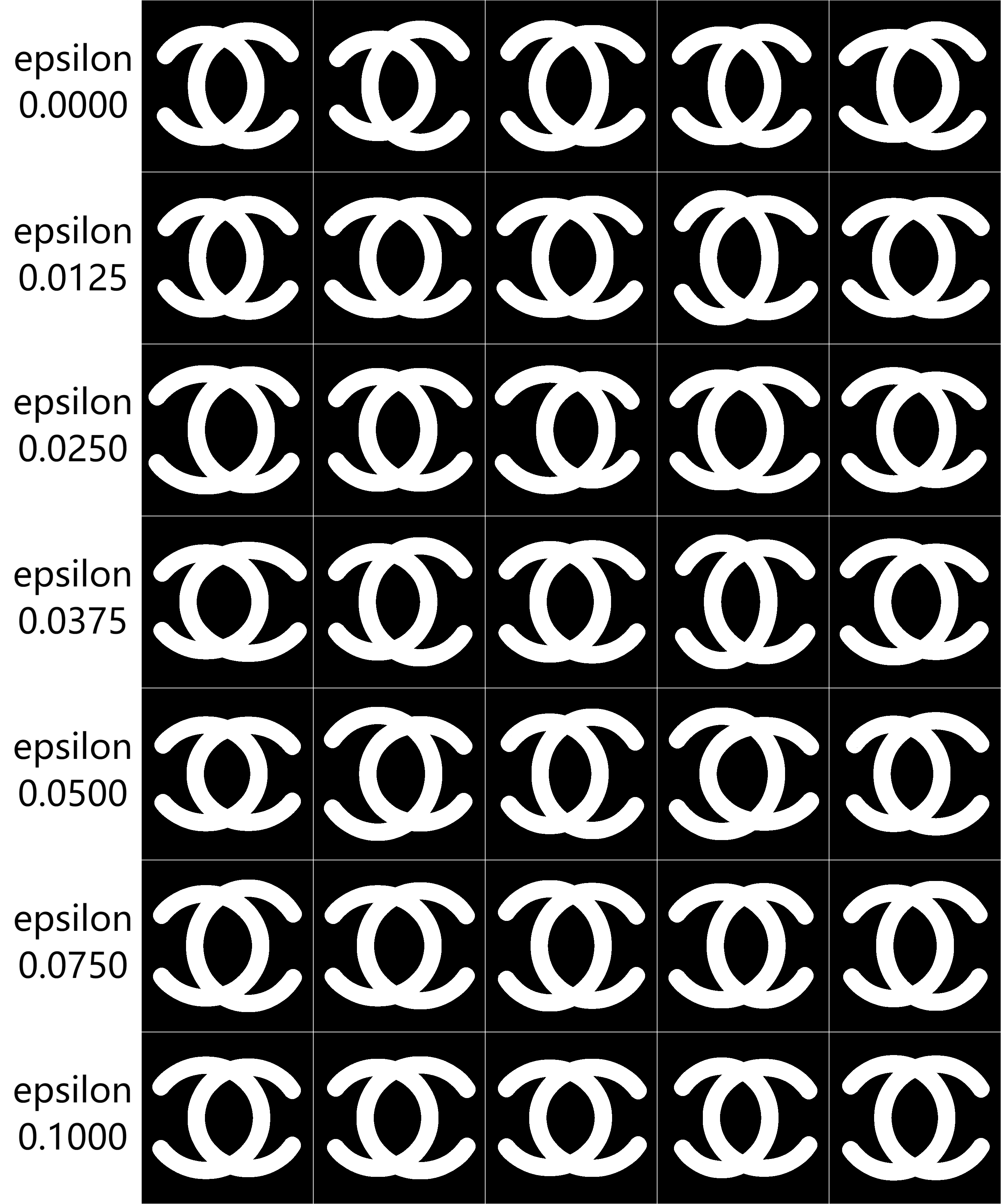
We conduct experiments by setting $T=3$ and directions $\nu_{p}=(\cos\frac{p-1}{4}\pi,\sin\frac{p-1}{4}\pi)^{T}$ for $p\in\{1,2,3,4\}$, sublevel sets with $t_{q}=\frac{T}{50}q=0.06q$ for $q\in\{1,\cdots,50\}$. We generate two collections of shapes, $\{K_{i}^{(0)}\}_{i=1}^{n}\overset{i.i.d.}{\sim}\mathbb{P}^{(0)}$ and $\{K_{i}^{(\varepsilon)}\}_{i=1}^{n}\overset{i.i.d.}{\sim}\mathbb{P}^{(\varepsilon)}$, independently for each $\varepsilon\in$ {0, 0.0125, 0.025, 0.0375, 0.05, 0.075, 0.1}, using Eq (3.1), with the number of shape pairs set to $n=100$ (here, we take balanced groups as a proof-of-concept example.). We then compute the ECT and SECT of each generated shape in directions $\{\nu_{p}\}_{p=1}^{4}$ and at levels $\{t_{q}\}_{q=1}^{50}$. Next, we implement Algorithms 1 and 2 (with input significance $\alpha=0.05$) on these computed ECT and SECT variables. We repeat this procedure 100 times and report the rejection rates for each epsilon across all 100 replicates in Table 1. Moreover, we visually present the rejection rates of Algorithms 1 and 2 in Figure 4.

Table 1: Rejection rates of Algorithms 1 and 2 across different indices $\varepsilon$. We assess the type I error rate of the different algorithms when the null model is true (i.e., $\varepsilon$ = 0). We then assess power of these approaches in the other cases.

Indices $\varepsilon$	0.000	0.0125	0.0250	0.0375
Rejection rates of ALGO 1	0.05	0.12	0.21	0.69
Rejection rates of ALGO 2	0.01	0.10	0.11	0.34
Indices $\varepsilon$	0.0500	0.0750	0.100	0.100
Rejection rates of ALGO 1	0.84	1.00	1.00	1.00
Rejection rates of ALGO 2	0.66	0.99	1.00	1.00

Figure 4: The plot in the top-left panel presents the relationship between $\varepsilon$ and the rejection rates computed via Algorithms 1 (black) and 2 (red) throughout all simulations. The x-axis shows the rejection rates corresponding to $\varepsilon\in\{0.0000,\,0.0125,\,0.0250,\,0.0375,\,0.0500,\,0.0750,\,0.1000\}$. A shape $K$ generated from $\mathbb{P}^{(0.075)}$ is presented in the top-right panel. In the second row presents the curves $t\mapsto\operatorname{SECT}(K)(\nu;t)$ for directions $\nu=(1,0)$ and $(0,1)$, respectively. The curves may be interpreted as 1-dimensional manifolds, suggesting a potential correlation between SECT and manifold learning (Meng and Eloyan, 2021b).

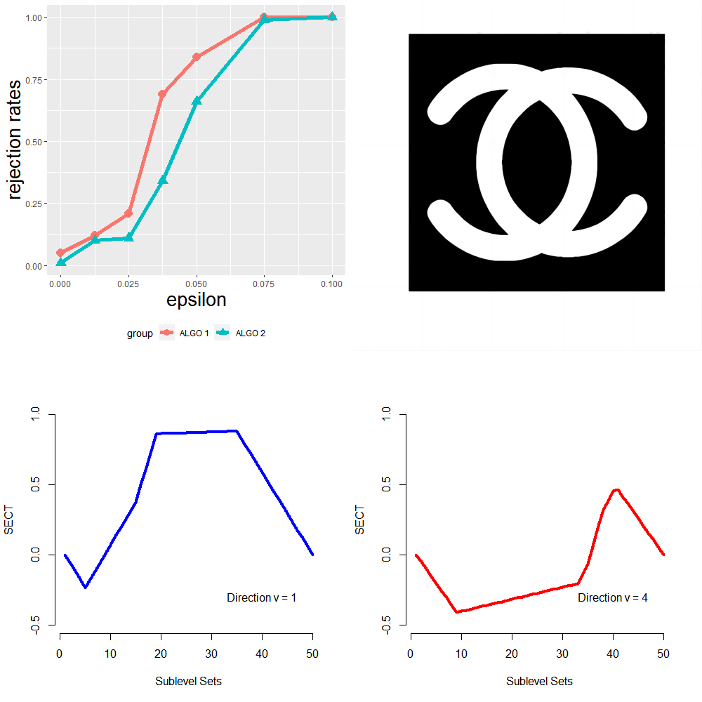
The simulation results demonstrate the effectiveness of our proposed Algorithm 1 in detecting the differences between $\mathbb{P}^{(\varepsilon)}$ and $\mathbb{P}^{(0)}$. Specifically, as the value of $\varepsilon$ increases, the rejection rates under the alternative hypothesis of Algorithm 1 also increase. And the power of Algorithm 2 under the alternative hypothesis is weaker compared to our proposed Algorithm 1. These findings highlight the superior performance of Algorithm 1 in detecting deviations between the two shape-generating distributions. In addition, the scenario in Table 1 where $\varepsilon=0$ indicates that our proposed Algorithm 1 does not suffer from type I error inflation, which is an inherent feature of a permutation test (recall that our input significance is $\alpha=0.05$).

4 Applications

In this section, we apply our proposed Algorithm 1 on the low-dose chest computed tomography (CT) images in a lung cancer dataset.

4.1 Application to Lung Cancer Imaging Dataset

CT scans of lung cancer tumors were collected from $n=685$ patients, archived by National Lung Screening Trial (NLST). Our analysis focused on a subset of this database, distinguishing between two nodule statuses: malignant and benign, as depicted in Figure 1. Each set (malignant or benign) of CT scans comprised 20 grayscale images, representing nodule lesions differentiated from the surrounding lung tissue. Subsequently, these grayscale images underwent thresholding to produce binary images. For each shape $K$ in the data set (i.e., a white region in Figure 1), we compute $\operatorname{SECT}(K)(\nu;t)$ for 72 directions $\nu=(\cos\phi,\sin\phi)$ with $\phi$ evenly sampled over the interval $[0,2\pi]$, using 100 sublevels $t$ in each direction. The code for implementing our Algorithm 1 in this subsection is built upon the materials in the GitHub repository of authors of Crawford et al. (2020). We modified the code to suit the analysis in this section. Example $\operatorname{SECT}$ summary statistics for a malignant nodule are presented in Figure 5. To test the hypothesis that malignant tumors exhibit significant differences compared to benign tumors, we utilized Algorithm 1, with the result presented in Table 2 (row 1) by a permutation p-value. Moreover, each dataset was randomly partitioned into two halves, and Algorithm 1 was subsequently applied to detect differences between the two halves. This procedure of random division was conducted 100 times, and the associated p-values, along with their mean and standard deviation, are presented in Table 2 (rows 4-5).

The results of implementing Algorithm 1, as outlined in Table 2 (row 1), underscore the capability of our proposed Algorithm 1 to differentiate between distinct nodule statuses. Conversely, rows 4-5 of Table 2 suggest that our algorithm refrains from erroneously distinguishing identical nodule statuses.

Table 2: P-values of Algorithm 1 for the lung cancer imaging dataset.

Malignant vs. Benign (Algorithm 1)	0.008
Malignant vs. Benign (ResNet18, logistic regression)	0.013
Malignant vs. Benign (ResNet18, $\chi^{2}$-test)	0.024
Malignant vs. Malignant	0.499 (0.300)
Benign vs. Benign	0.511 (0.306)

Figure 5: Example of a malignant nodule (left), denoted by $K$, with its SECT curves (right). In the right panel, we illustrate the curves $t\mapsto\operatorname{SECT}(K)(\nu,t)$ for three different directions $\nu$.

4.2 Comparative Analysis of the NHST-SECT Algorithm and Conventional Artificial Neural Network Model

In this subsection, we compare our proposed NHST-SECT method (Algorithm 1) to a state-of-the-art artificial neural network model, focusing on their performance in the lung cancer images presented in Figure 1. We chose the widely used ResNet18 architecture implemented in PyTorch (He et al., 2015). We adopted a leave-one-out approach. Specifically, (i) we trained the ResNet18 model on a dataset consisting of 39 CT images, with one image held out for testing in each iteration; (ii) subsequently, the trained model was applied to the held-out image to predict the malignant/benign label of the image (recall that the true label is available); (iii) we iterated this procedure 40 times, with a distinct image held out in each iteration. Consequently, after completing the 40 iterations, each individual image possessed two labels denoting its malignancy/benignity status: the true label and the label predicted through the application of the corresponding trained ResNet18 model. The prediction results via ResNet18 can be found in Figure 6, presented in the form of a $2\times 2$ contingency table. We firstly employed logistic regression, regressing the true labels against the predicted labels, subsequently obtaining the p-value associated with the regression coefficient. We also conducted $\chi^{2}$-test (see Shao (2003), Section 6.4.3 therein) and obtained the corresponding $\chi^{2}$-derived p-value. The ResNet18-derived p-values (0.013 for logistic regression, and 0.024 for $\chi^{2}$-test) are presented in rows 2-3 of Table 2, indicating that our proposed NHST-SECT method is comparable with the state-of-the-art ResNet18 model.

Figure 6: The prediction results of ResNet18 model.

Our proposed Algorithm 1 enjoys several notable advantages over conventional artificial neural network models for medical image classification:

1. Interpretability and Mathematical Foundation. Unlike the black-box nature of the artificial neural network models, our method is grounded in sound mathematical and statistical theories, providing a clear and interpretable basis.

2. Efficient Computational Performance. Efficiency is a critical consideration in medical image analysis, and our method offers reasonable computational efficiency. With a time complexity of $O(n)$, where $n$ represents the number of medical images, our algorithm completed all the data analyses presented in Section 4.1 in approximately 50 seconds (on a computer with an AMD Ryzen 7 5800H processor running at 3200 MHz using 16 GB of RAM). This efficiency rivals popular artificial neural network models, making our method a viable and competitive alternative.

3. Robust Performance on Small Datasets. Medical image datasets are often limited in size due to the precious nature of the data. Conventional artificial neural network models are susceptible to overfitting on such small datasets, leading to erroneous classifications on the test set. Due to the permutation technique (recall the discussion at the beginning of Section 2.2), our proposed method does not suffer from small sample sizes.

5 Conclusion and Future Research

We introduced the randomization-style NHST-SECT algorithm (Algorithm 1) for detecting significance differences between shape collections. Simulation studies showed the promising performance of our algorithm. As proof of concept, we applied our proposed algorithm to a dataset of lung cancer images.

Similar methods can be potentially applied to analyze human brain functional connectivity (Lindquist, 2008, Meng and Eloyan, 2021a), e.g., detecting significant differences between two collections of functional connectivity structures, which is left for our future research.

DATA AVAILABILITY STATEMENT

The source code for implementing the simulation studies is publicly available online in the GitHub repository https://github.com/JinyuWang123/NHST-SECT.git. Due to privacy and confidentiality considerations, the data set utilized in Section 4 cannot be made publicly available.

Appendix: ECT-based Randomization-style Null Hypothesis Significance Test

The SECT originated from the Euler characteristic transform (ECT, Turner et al. (2014)) defined as follows

$$\begin{aligned} &\operatorname{ECT}:\ \ K\mapsto\{\operatorname{ECT}(K)(\nu;t)\}_{(\nu,t)\in\mathbb{S}^{d-1}\times[0,T]},\\ &\text{where }\ \ \ \operatorname{ECT}(K)(\nu;t)=\chi(K_{t}^{\nu}).\end{aligned}$$

In Section 3, we compared our proposed Algorithm 1 with the “ECT-based randomization-style null hypothesis significance test” (see Meng et al. (2022) and Section 5.3 of Robinson and Turner (2017)), which is based on permutation test and the following loss functional

$$\begin{aligned} H\left(\{K_{i}^{(1)}\}_{i=1}^{n_{1}},\,\{K_{i}^{(2)}\}_{i=1}^{n_{2}}\right)\overset{\operatorname{def}}{=}\sum_{j=1}^{2}\frac{1}{2n_{j}(n_{j}-1)}\sum_{k,l=1}^{n_{j}}\theta\left(K_{k}^{(j)},\,K_{l}^{(j)}\right),\end{aligned}$$ (.1)

where $\theta$ is the dissimilarity function defined by the following

$$\theta\left(K^{(1)},K^{(2)}\right)=\sup_{\nu\in\mathbb{S}^{d-1}}\left\{\left(\int_{0}^{T}\left|\,\operatorname{ECT}(K^{(1)})(\nu;t)-\operatorname{ECT}(K^{(2)})(\nu;t)\,\right|^{2}dt\right)^{1/2}\right\}.$$

For a given discretized ECT denoted by $\{ECT(K_{i}^{(j)})(\nu_{p};t_{q}):p=1,\cdots,\Gamma\mbox{ and }q=1,\cdots,\Delta\}_{i=1}^{n}$, applying the strategy in Eq. (2.7), we may adopt the following test statistics to approximate the loss functional in Eq. (.1)

$$\begin{aligned} &\theta\left(K_{k}^{(j)},\,K_{l}^{(j)}\right)\approx\widehat{\theta}\left(K_{k}^{(j)},\,K_{l}^{(j)}\right)\overset{\operatorname{def}}{=}\sup_{p=1,\ldots,\Gamma}\left(\sum_{q=1}^{\Delta}\left|\,\operatorname{ECT}(K_{k}^{(j)})(\nu_{p};t_{q})-\operatorname{ECT}(K_{l}^{(j)})(\nu_{p};t_{q})\,\right|^{2}\right)^{1/2},\\ &H\left(\{K_{i}^{(1)}\}_{i=1}^{n_{1}},\,\{K_{i}^{(2)}\}_{i=1}^{n_{2}}\right)\approx\widehat{H}\left(\{K_{i}^{(1)}\}_{i=1}^{n_{1}},\,\{K_{i}^{(2)}\}_{i=1}^{n_{2}}\right)\overset{\operatorname{def}}{=}\sum_{j=1}^{2}\frac{1}{2n_{j}(n_{j}-1)}\sum_{k,l=1}^{n_{j}}\widehat{\theta}\left(K_{k}^{(j)},\,K_{l}^{(j)}\right)\end{aligned}$$ (.2)

The ECT-based randomization-style null hypothesis significance test is implemented using Algorithm 2.

Algorithm 2 : ECT-based randomization-style null hypothesis significance test

1:Input: (i) Discretized ECT of two collection of shapes $\{\operatorname{ECT}(K_{i}^{(j)})(\nu_{p};t_{q}):p=1,\cdots,\Gamma\mbox{ and }q=1,\cdots,\Delta\}_{i=1}^{n}$ for $j\in\{1,2\}$; (ii) desired confidence level $1-\alpha$ with significance $\alpha\in(0,1)$; (iii) the number of permutations $\Pi$.

2:Output: Accept or Reject the null hypothesis $H_{0}$ in Eq. (2.3).

3:Apply Eq. (.2) to the original input ECT data and compute the value of the loss $\mathfrak{S}_{0}\overset{\operatorname{def}}{=}\widehat{H}(\{K_{i}^{(1)}\}_{i=1}^{n},\,\{K_{i}^{(2)}\}_{i=1}^{n})$.

4:for all $k=1,\cdots,\Pi$,

5:Randomly permute the group labels $j\in\{1,2\}$ of the input ECT data.

6:Apply Eq. (.2) to the permuted ECT data and compute the value of the loss $\mathfrak{S}_{k}\overset{\operatorname{def}}{=}\widehat{H}(\{K_{i}^{(1)}\}_{i=1}^{n},\,\{K_{i}^{(2)}\}_{i=1}^{n})$.

7:end for

8:Compute $k^{*}\overset{\operatorname{def}}{=}[\alpha\cdot\Pi]\overset{\operatorname{def}}{=}$ the largest integer smaller than $\alpha\cdot\Pi$.

9:Reject the null hypothesis $H_{0}$ if $\mathfrak{S}_{0}<\mathfrak{S}_{k^{*}}$ and report the output.

References

- Bankman (2008) I. Bankman. Handbook of medical image processing and analysis. Elsevier, 2008.
- Brezis (2011) H. Brezis. Functional analysis, Sobolev spaces and partial differential equations, volume 2. Springer, 2011.
- Carlsson (2009) G. Carlsson. Topology and data. Bulletin of the American Mathematical Society, 46(2):255–308, 2009.
- Crawford et al. (2020) L. Crawford, A. Monod, A. X. Chen, S. Mukherjee, and R. Rabadán. Predicting clinical outcomes in glioblastoma: an application of topological and functional data analysis. Journal of the American Statistical Association, 115(531):1139–1150, 2020.
- Edelsbrunner and Harer (2022) H. Edelsbrunner and J. L. Harer. Computational topology: an introduction. American Mathematical Society, 2022.
- Edelsbrunner et al. (2000) H. Edelsbrunner, D. Letscher, and A. Zomorodian. Topological persistence and simplification. In Proceedings 41st annual symposium on foundations of computer science, pages 454–463. IEEE, 2000.
- Ghrist et al. (2018) R. Ghrist, R. Levanger, and H. Mai. Persistent homology and Euler integral transforms. Journal of Applied and Computational Topology, 2(1):55–60, 2018.
- Good (2013) P. Good. Permutation tests: a practical guide to resampling methods for testing hypotheses. Springer Science & Business Media, 2013.
- Hatcher (2002) A. Hatcher. Algebraic Topology. Cambridge University Press, 2002.
- He et al. (2015) K. He, X. Zhang, S. Ren, and J. Sun. Deep residual learning for image recognition. 2016 IEEE Conference on Computer Vision and Pattern Recognition (CVPR), pages 770–778, 2015.
- Lindquist (2008) M. A. Lindquist. The statistical analysis of fmri data. 2008.
- Maldonado et al. (2021) F. Maldonado, C. Varghese, S. Rajagopalan, F. Duan, A. B. Balar, D. A. Lakhani, S. L. Antic, P. P. Massion, T. F. Johnson, R. A. Karwoski, R. A. Robb, B. J. Bartholmai, and T. Peikert. Validation of the broders classifier (benign versus aggressive nodule evaluation using radiomic stratification), a novel hrct-based radiomic classifier for indeterminate pulmonary nodules. European Respiratory Journal, 57(4), 2021. ISSN 0903-1936.
- Marsh et al. (2022) L. Marsh, F. Y. Zhou, X. Quin, X. Lu, H. M. Byrne, and H. A. Harrington. Detecting temporal shape changes with the Euler characteristic transform. arXiv preprint arXiv:2212.10883, 2022.
- Meng and Eloyan (2021a) K. Meng and A. Eloyan. Population-level task-evoked functional connectivity via fourier analysis. arXiv e-prints, pages arXiv–2102, 2021a.
- Meng and Eloyan (2021b) K. Meng and A. Eloyan. Principal manifold estimation via model complexity selection. Journal of the Royal Statistical Society: Series B (Statistical Methodology), 83(2):369–394, 2021b.
- Meng et al. (2022) K. Meng, J. Wang, L. Crawford, and A. Eloyan. Randomness and statistical inference of shapes via the smooth Euler characteristic transform. arXiv preprint arXiv:2204.12699, 2022.
- Pike et al. (2019) J. Pike, A. Khan, C. Pallini, S. Thomas, M. Mund, J. Ries, N. Poulter, and I. Styles. Topological data analysis quantifies biological nano-structure from single molecule localization microscopy. Bioinformatics (Oxford, England), 36, 10 2019.
- Robinson and Turner (2017) A. Robinson and K. Turner. Hypothesis testing for topological data analysis. Journal of Applied and Computational Topology, 1, 12 2017.
- Shao (2003) J. Shao. Mathematical statistics. Springer Science & Business Media, 2003.
- Turner et al. (2014) K. Turner, S. Mukherjee, and D. M. Boyer. Persistent homology transform for modeling shapes and surfaces. Information and Inference: A Journal of the IMA, 3(4):310–344, 2014.
- Wang et al. (2021) B. Wang, T. Sudijono, H. Kirveslahti, T. Gao, D. M. Boyer, S. Mukherjee, and L. Crawford. A statistical pipeline for identifying physical features that differentiate classes of 3d shapes. The Annals of Applied Statistics, 15(2):638–661, 2021.
- Wang et al. (2016) J.-L. Wang, J.-M. Chiou, and H.-G. Müller. Functional data analysis. Annual Review of Statistics and its application, 3:257–295, 2016.
- Wasserman (2018) L. Wasserman. Topological data analysis. Annual Review of Statistics and Its Application, 5:501–532, 2018.