Contagion Effects of the Silicon Valley Bank Run

Abstract

This paper analyzes the contagion effects associated with the failure of Silicon Valley Bank (SVB) and identifies bank-specific vulnerabilities contributing to the subsequent declines in banks’ stock returns. We find that uninsured deposits, unrealized losses in held-to-maturity securities, bank size, and cash holdings had a significant impact, while better-quality assets or holdings of liquid securities did not help mitigate the negative spillovers. Interestingly, banks whose stocks performed worse post-SVB also experienced lower returns in the previous year, following Federal Reserve interest rate hikes. Stock investors appeared to anticipate risks associated with uninsured deposit reliance, but did not foresee the realization of implied losses. While mid-sized banks experienced particular stress immediately after the SVB failure, over time negative spillovers became widespread except for the largest banks.

Keywords: Contagion, Banking crisis, Bank run, Systemic risk, Interest rate risk, Hidden losses, Held-to-maturity

JEL Codes: G01, G21, G14, G28, E58, E43

1 Introduction

On March 10th, 2023, Silicon Valley Bank (SVB) failed after a bank run. It was the sixteenth largest bank in the United States as of the end of 2022, with $209 billion in assets, which marked the largest bank failure since the Global Financial Crisis (GFC) of 2007-2009 and the second-largest bank failure in U.S. history, second only to Washington Mutual. As a response, a “systemic risk exception” was invoked by the policymakers, leading to a blanket guarantee on all deposits at SVB. The failure of SVB, the subsequent bank failures, and the policy responses, such as the blanket deposit guarantee and the new central bank lending facility, underscore the continued significance of bank runs and contagion as important features of the global financial system, even after the implementation of regulatory reforms following the GFC.

Financial contagion can propagate through various channels. These include direct exposures via interbank linkages, information spillovers where difficulties of one bank can be interpreted as a negative signal for others, and disorderly liquidations of illiquid assets. Identifying banks that are affected by contagion during a financial crisis can help delineate the underlying mechanisms driving systemic risk. Market responses, such as measured by changes in stock prices, provide valuable information for quantifying the impact of contagion on other banks. This study adopts the approach of [29], which analyzed contagion associated with the failure of Northern Rock in the United Kingdom during the GFC. Specifically, we examine the stock price reactions of banks following the switch to tighter monetary policy and the subsequent failure of SVB to characterize which specific bank characteristics played a significant role in driving the spillovers.

In response to historic levels of U.S. inflation following the COVID-19 pandemic, the Federal Reserve began to increase its policy rate on March 17, 2022. While rate hikes were initially expected to benefit the banking sector by allowing higher net interest margins for new loans ([22]), they also introduced vulnerabilities associated with duration mismatch for existing fixed-rate assets.

SVB was particularly exposed to duration risk due to a majority of its investments in highly-rated government bonds with very long maturities. By the end of 2022, SVB’s bond portfolio consisted of $91.3 billion in held-to-maturity (HTM) and $26.1 billion in available-for-sale (AFS) assets, with marked-to-market accounting unrealized losses for its HTM securities exceeding $15 billion. However, these losses were considered “potential” and would only materialize if the bank was forced to sell the assets during liquidity stress events such as heavy deposit withdrawals. Amidst mounting concerns, SVB experienced a steady decline in deposits over the four quarters leading up to its eventual failure. The pace of withdrawals intensified during the week of March 6th, 2023, culminating in an abrupt outflow of $42 billion on a single day, March 9th. The run on SVB triggered its failure and subsequent takeover by FDIC on March 10th ([37]).

The run on SVB triggered significant spillover effects on the U.S. banking system. One crucial factor that contributed to the spillover effects was the concern over unrealized losses in highly liquid securities. Unlike typical bank run scenarios, where liquid assets act as buffers, the realization of losses on the liquid securities due to funding outflows proved problematic. Having more liquid securities did not help mitigate contagion; only cash holdings were effective. Additionally, reliance on uninsured deposits exacerbated financial distress due to their potential for rapid withdrawal.

The correlation of bank size with spillover effects was also noteworthy. Mid-sized banks, particularly those with assets in the $50 billion to $250 billion range referred to as “super-regional” banks, experienced heightened stress immediately after the run on SVB. These banks had previously been designated as systemically important by the regulators but faced relaxed regulations after the 2019 regulatory rollback. Investors initially exhibited greater concerns with banks of a similar size to SVB, potentially due to regulatory differences. Over the next months, however, the negative effects spread to other banks as concerns about the entire banking system became more widespread. Surprisingly, very large banks, particularly those with assets over $1 trillion, outperformed the rest of the system. This may be attributed to implicit too-big-to-fail (TBTF) guarantees and consequent deposit inflows, since these banks were perceived as safe havens during the systemic instability ([11], [39]).

Market participants also seemed to anticipate these banks’ vulnerabilities, as the same banks that suffered more after the SVB failure had also underperformed in the previous year. We investigate which vulnerabilities were anticipated, and which came as a “surprise” following the failure of SVB. It is important to note that all information we use, including the unrealized losses in hold-to-maturity securities, was available to the market in January 2023 through public regulatory filings. Our analysis suggests that market participants had already factored in vulnerabilities associated with reliance on uninsured deposits and limited cash holdings.

However, damages from implied losses and the impact of bank size were more of a surprise. If depositors do not perceive implied losses as problematic and do not run on the bank, stock investors may have had little reason to worry about them. Although, this changed abruptly with the failure of SVB, which aligns with the information view of banking panics ([18]), where bank runs are caused by abrupt shifts in depositors’ risk perceptions. The sudden realization of risks in bank assets can be triggered by an arrival of new information such as the failure of a large institution or negative news on aggregate fundamentals ([31]).

The SVB episode has some similarities with the Savings and Loans (S&L) crisis and the GFC, but also important differences. When inflation reached historic levels in the United States, the Federal Reserve started to increase interest rates in October 1979. S&Ls specialized in residential mortgages and issued long-term fixed-rate loans. This exposed S&Ls to significant interest rate risk like SVB.However, unlike the 2023 crisis, where rapid depositor runs played a critical role, S&L crisis was a relatively slow-moving process. Faced by mounting losses, regulators relaxed regulation and exercised forbearance, hoping the S&Ls could outlast out of their balance sheet problems. This gave S&Ls the opportunity to gamble for resurrection, resulting in excessive risk taking and imprudent real estate lending. Over time, what started from interest rate risk turned into a crisis of bad loans and credit risk.

During the GFC, low quality loans, complexity of financial products and the runs in wholesale funding markets played a major role. The new regulatory framework of Basel III has tried to address the fragility of wholesale funding by giving favorable treatment for deposits, which were viewed as a more stable source of funding. The SVB episode showed us that uninsured deposits can also be a major source of bank runs. Moreover, even the safest and most liquid securities like Treasuries can also experience significant losses due to interest rate risk. While hold-to-maturity accounting can hide these losses on banks’ balance sheets, the losses can crystallize when banks are forced to sell the securities at market prices when faced with urgent liquidity needs.

Overall, the unrealized losses in securities, the vulnerability of uninsured deposits to runs, and the interaction between the two were new factors during this baking episode. The ex-ante neglect by investors further underscores the challenges for policymakers in crafting robust stress scenarios that comprehensively account for all pertinent vulnerabilities beforehand. These are important insights for policy makers and will help them in designing new policies to make the financial system more resilient.

Related literature: The paper is related to the vast literature on bank runs (e.g., [20], [14], [13], [3], and [30]) and their origins ([31], [12]). It also contributes to the literature on the channels of contagion, such as direct exposures via interbank linkages ([4]); information contagion ([15], [1]); and illiquidity and asset prices ([21], [32], and [16]).

The paper is also related to the literature on banks’ interest rate risk. A recent study by [23] suggests that banks’ deposit franchise can act as a natural hedge against interest rate risks, while [24] argue that a bank run equilibrium can emerge when banks heavily rely on uninsured deposits during rate increases. Investigating the 2022 monetary tightening period, [36] find significant exposures to interest rate risk with limited use of hedging (see also [7]).

Several other studies examine the implications of SVB’s failure and the subsequent banking crisis. [37] document substantial mark-to-market losses spread across the banking sector, which is also confirmed by [26]. They assess the impact of the run by uninsured depositors leading to bank insolvency due to the realization of these potential losses. [33] present a theoretical model that characterizes the role of rapid rate hikes in bringing this vulnerability and offer empirical evidence supporting their predictions. [11] present findings on depositors’ flight to safety, whereby funds shift away from regional banks towards larger banks.

In contrast to papers that focus on the effect of a specific factor on contagion, our study provides a comprehensive assessment of multiple factors contributing to negative spillovers. We emphasize the unique characteristics of the 2023 crisis compared to the GFC, offering valuable insights for regulatory objectives. Additionally, our analysis distinguishes between the immediate and medium-term effects, uncovering the emergence of the too-big-to-fail effect as concerns spread across the entire banking system. Finally, we find that investors partially anticipated vulnerabilities associated with uninsured deposits, but other factors, such as those related to unrealized losses and bank size, appeared to come as a surprise.

2 Background and Conceptual Framework

First, we provide a background and a summary of the events that led to the failure of SVB. Then, we discuss the factors that might have played a role in the failure of SVB such as interest rate risk and implied losses, liquidity risk and unsecured deposits, and the rollback of regulation.

2.1 A summary of the SVB failure

SVB was founded in 1983 with a focus on the needs of startup companies. Its main strategy was to collect deposits from businesses financed through venture capital while it expanded into banking and financing venture capitalists. During the 1980s, SVB grew with the local high-tech economy and experienced significant growth during the 1990s, where the computer technology startups during the dot-com bubble provided an influx of business for the bank. In the 2000s, SVB entered into the private banking business building on earlier experience and relationships with wealthy venture capitalists and entrepreneurs, and enjoyed an international expansion which continued in the 2010s. In 2015, the bank stated that it served 65% of all U.S. startups.

During the loose monetary policy of the pandemic-era and the investment boom in private technology companies, SVB enjoyed a significant increase in its deposits and asset size, where, just in 2021, deposits surged from $102 billion to $189 billion. Awashed with deposits, SVB increased its investment in highly-rated government bonds in its portfolio to $120 billion of which $91 billion consisted of fixed-rate mortgage bonds with very long maturities. This, in turn, exposed SVB to interest rate risk. On the liability side, regulatory filings estimated that more than 90% of its deposits were uninsured, which exposed the bank to funding liquidity risk and a depositor run.

In response to the spike in inflation following the COVID-19 pandemic, the Federal Reserve began to increase interest rates in March 2022. This led to SVB incurring heavy losses on its bond portfolio. While SVB deposits dropped for four straight quarters prior to its failure, deposit withdrawal was faster than expected in February and March of 2023. As a result, SVB had to liquidate its HTM assets, and incurred a loss of $1.8 billion. To cover these losses, SVB announced a capital raise of $2.25 billion in the week of its failure. On March 8th Moody’s downgraded SVB and it was apparent on March 9th that SVB was not being able to raise the needed capital. This exacerbated a depositor run with withdrawals of $42 billion, equal to a quarter of bank deposits, on a single day. On March 10th, SVB failed as a result of the bank run and was put into receivership by the FDIC. On March 12th, in a joint statement by the Secretary of the Treasury, Federal Reserve Chairman and the FDIC Chairman, a blanket guarantee for insured and uninsured deposits at SVB was introduced.

2.2 Factors

In this section, we discuss factors which had a role in the failure of SVB and the subsequent spillover effects such as interest rate risk and implied losses, liquidity risk arising from uninsured deposits, and an erosion of the regulatory framework governing mid-sized banks.

2.2.1 Interest rate risk and implied losses

To combat inflation, the Federal Reserve began hiking interest hikes in March 2022. SVB had significant exposure to interest rate risk in its bond portfolio. SVB’s bond portfolio was separated into HTM and AFS securities. HTM securities are planned to be held until maturity and can be carried at their nominal par value since they are being held until they are repaid in full. On the other hand, AFS securities are marked to market. At the end of 2022, SVB had $91.3 billion in HTM securities with very long maturities and $26.1 billion on AFS securities. Increasing interest rates led to losses in the market value of its bonds with significant unrealized losses for its HTM securities. The rise in interest rates and the resulting losses in the securities portfolio of SVB, some of which were hidden due to the HTM assets, was a major contributor in the demise of SVB ([37]).

2.2.2 Liquidity risk due to unsecured deposits

During the GFC of 2007-08, a key lesson learned was the importance of differentiating between wholesale funding and deposits when assessing funding risk. While wholesale funding was highly vulnerable to runs during the crisis, deposits turned out to be relatively “sticky” and less likely to be withdrawn by panicked investors (see, e.g., [35] and [34]). This insight has been incorporated into regulatory reforms aimed at improving the resilience of the banking system such as the Liquidity Coverage Ratio (LCR) requirement of Basel III ([6]). In particular, the LCR requirement mandates that banks must have sufficient high quality liquid assets (HQLA) to meet net cash outflows for 30 days under a stress scenario. SVB’s bond portfolio, which constituted a major part of its assets, would be considered as HQLA in the context of LCR. Nevertheless, the securities in its portfolio had interest rate risk exposure. Even though both cash and most of the securities were treated to be highly liquid in the LCR framework, cash ended up being significantly more valuable to banks, as we discuss in Section 4.2.2.

LCR assumes a lower outflow rate for deposits than for market funding, reflecting the greater stability and reliability of deposit funding. SVB largely financed itself via uninsured deposits, which turned out to be subject to severe runs even though they were expected to be less “flighty” compared to other wholesale funding sources under LCR. Heavy reliance on uninsured deposits exposed SVB to funding liquidity risk. As we argued above, potential losses becoming actual losses due to deposit withdrawals played a crucial role in the demise of SVB.

2.2.3 Rolling back regulation for mid-sized banks

After the GFC, the Dodd-Frank Act provided a major reform for the regulatory framework. However, on May 24th, 2018, The Economic Growth, Regulatory Relief, and Consumer Protection Act (S. 2155) was signed into law and eased the regulations for mid-sized banks by raising the threshold for systemically important financial institutions from $50 billion to $250 billion. One consequence of the regulatory rollback was that SVB was not subject to the LCR requirement. Furthermore, despite interest rate risk being the major factor in the failure of SVB, regulatory stress tests did not incorporate an interest rate risk scenario.

3 Data and Methods

3.1 Data

We start with the Federal Reserve Bank of New York’s permanent company number (PERMCO)-RSSDID crosswalk. This crosswalk provides the PERMCO identifier for most regulated banks in the United States. Using the Center for Research in Security Prices (CRSP) database, we link the PERMCO to each firm’s stock ticker as of 2022q4. The linked list dataset of RSSDID and tickers has 327 banks.

Next, we construct a dataset using these tickers of daily close stock price data from Yahoo! Finance for February 1, 2022 until May 25, 2023. We are able to pull this data for 324 of the tickers. We construct daily returns based on these measures, and a measure of market returns based on close price of the S&P 500. We also construct a daily return measure for banks based on the Dow Jones U.S. Banks Index (DJUSBK).

Then, for each of the 327 RSSDIDs in our initial list, we identify all subsidiaries of the bank using the National Information Center (NIC)’s relationship file. For each subsidiary, if they are regulated by the FDIC, we identify their FDIC Certificate Number, and collect their total deposits, total uninsured deposits, and total assets using the FDIC’s BankSuite tool. This is a sample of 318 top holders and banks.

Finally, for those top holder companies who report FR Y-9C data and for commercial banks that report Call Report data, we construct several financial balance sheet measures from their 2022q4 report. These include total assets, cash, securities, HTM and AFS securities, mark-to-market losses on HTM securities based on the difference between their book values and fair values, Tier 1 capital, and non-performing loans. This is a sample of 224 top holders and banks. Our final sample is described in Table 1. For several of our banks, neither their regulatory Tier 1 capital ratios nor amounts of Tier 1 capital are reported. In regressions using these measures, we lose 2 and 8 observations, respectively.

Table 1: Sample Composition and Summary Statistics. This table reports summary statistics of the main bank characteristics in our sample, measured as of 2022q4.

Variable Observations Mean Median SD Assets (000) 224 101,688,402 9,559,211 405,970,115 Cash / Assets 224 9.2% 8.1% 7% Securities / Assets 224 20% 18% 11% Liquid Assets / Assets 224 29% 27% 13% Unrealized HTM Losses / Tier 1 Capital 222 0.21% 0% 2.2% Hold-to-Maturity Securities / Assets 224 3.2% 0.33% 5.9% Uninsured Deposit Share 224 39% 38% 18% Tier 1 Capital Ratio 216 13% 12% 2.9%

3.2 Cumulative Returns in Excess of the S&P 500

We construct daily returns $r_{it}$ for each bank $i$ in period $t$ using the close price for each day. We then construct two sets of cumulative returns starting from February 1, 2023 and February 1, 2022 (referred to as “2023 returns” and “2022 returns,” respectively):

$$R^{2023}_{it}=\prod_{t^{\prime}\geq 2023-02-01}(1+r_{it^{\prime}})-1$$ (1)

$$R^{2022}_{it}=\prod_{t^{\prime}\geq 2022-02-01}(1+r_{it^{\prime}})-1$$ (2)

We then consider the excess return for this cumulative return above the cumulative return of the S&P 500 over the same time period (denoted as $R^{m,2023}_{it}$ and $R^{m,2022}_{it}$, respectively).

$$\tilde{R}^{2023}_{it}=R^{2023}_{it}-R^{m,2023}_{it}$$ (3)

This measure can be interpreted as the cumulative return difference between investing a dollar long in bank $i$ and a dollar short in the S&P500 on February 1, and holding the position. This differs slightly from traditional event study approaches by focusing on excess geometric returns, rather than arithmetic excess returns.

We consider how the $\tilde{R}_{it}$ corresponds to various bank-level characteristics using linear regressions. These regressions are run in the cross-section, using robust standard errors.

4 Results

We first present the overall trends in bank stock returns since the commencement of the rate hikes by the Federal Reserve in early 2022. Next, we analyze the vulnerability factors associated with spillover effects following the SVB failure. Finally, we discuss whether market participants had anticipated such vulnerabilities ex ante.

4.1 Overall trends

Figure 1 displays the cumulative returns for the S&P 500 index and the banking sector. The top panel plots the 2022 returns to illustrate the trends observed over the 12 months preceding the SVB’s failure, while the bottom panel shows the 2023 returns focusing on the subsequent 3 months after the event. We plot two measures of banking sector return: the Dow-Jones U.S. Bank Index (DJUSBK) and the asset-weighted average of our sample banks. The two sectoral returns exhibit a correlation of 0.99 in 2022.

Figure 1: Aggregate cumulative returns for the S&P 500 and banking sector. This figure plots cumulative returns for three sets of stock indices: the S&P 500 index, the Dow Jones U.S. Banks Index, and the asset-weighted average of the banks in our sample. The top panels reports the cumulative return starting in February 1, 2022, until January 31, 2023. The bottom panel reports the cumulative return from February 1, 2023, until May 25, 2023.

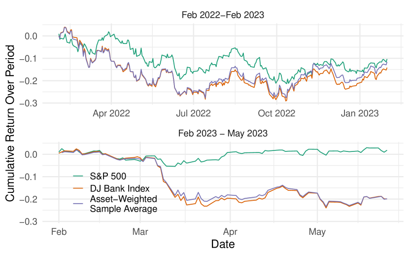
Since the start of the rate hikes on March 17, 2022, there was a general decline in stock prices. Notably, the banking sector initially exhibited even weaker performance compared to the rest of the market, as indicated in the top panel. However, this trend partially reversed later in the same year as the stock market started to recover. By early 2023, the cumulative impact of rate hikes was similar for banks and the overall market.

Following the bank run of SVB in March 2023, the relative performance of the banking sector diverged sharply from the rest of the market, as depicted in the bottom panel of Figure 1. While the S&P index did not show distinct signs of stress following the SVB failure, the banking sector as a whole declined by 20%. Furthermore, in Figure 2, which plots individual banks’ 2023 returns in the same time period as the Panel B of Figure 1, we observe a noticeable increase in cross-sectional variation in banks’ stock performance after the SVB bank run. The distribution of bank stock returns remained relatively tight prior to the FDIC takeover of SVB but widened significantly afterwards, indicating the presence of heterogeneous spillover effects. We highlight the eight banks with the largest declines as of March 17th. Some of these banks, including SVB and Signature Bank (SBNY), did not post market prices following their FDIC takeovers until later, and hence had fixed prices for several days. Several other banks, notably First Republic (FRC), also experienced substantial immediate declines. Our empirical analysis primarily aims to identify the factors contributing to these differential spillovers.

Figure 2: Bank Returns Over Time for Select Banks. This figure plots cumulative returns in excess of the S&P 500 index from February 1, 2023, until May 25, 2023. We highlight the 8 banks with the largest cumulative declines as of March 17th and the Dow Jones U.S. Bank Index’s abnormal returns. The rest of the banks in our sample are plotted in grey. Stocks are denoted by their ticker symbol; Silicon Valley Bank’s ticker is SIVB.

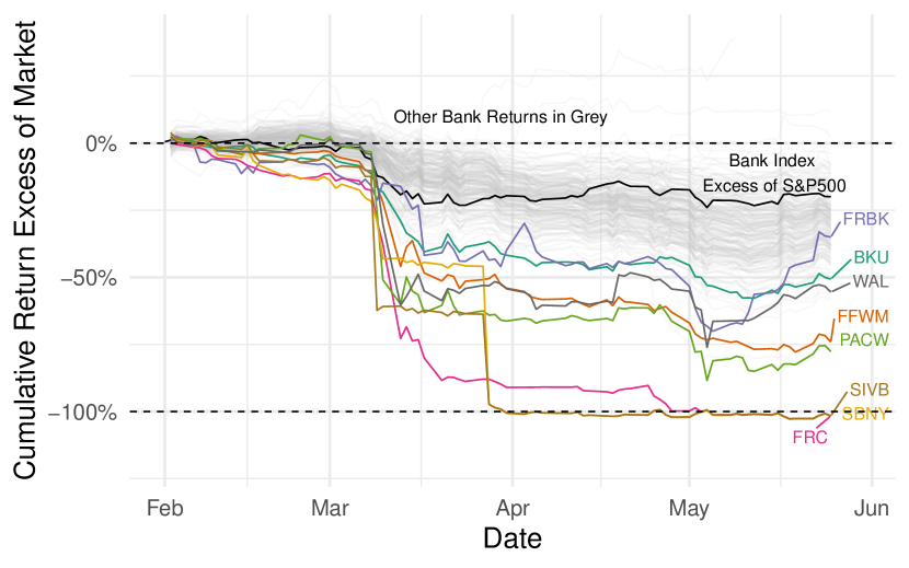
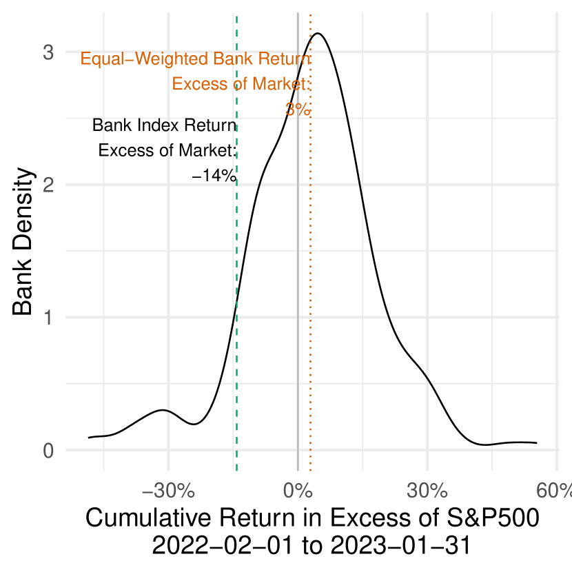
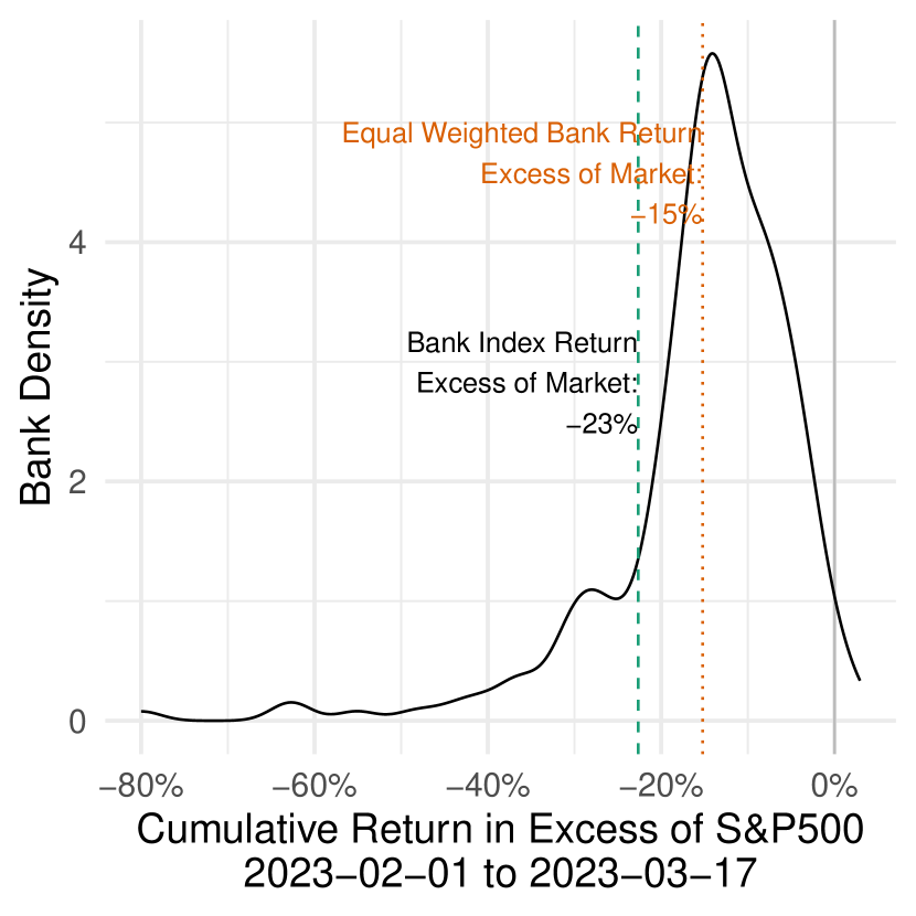
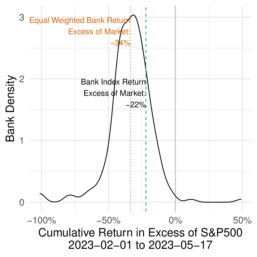
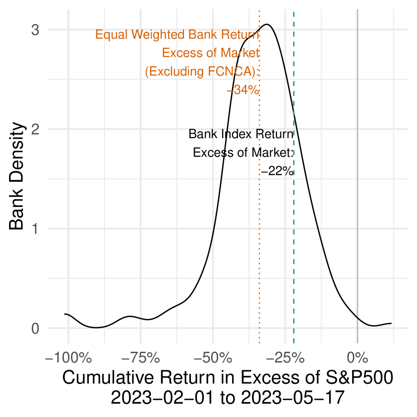
Figure 3 plots the full distribution of bank stock returns assessed across different time periods. Panel 3(a), based on cumulative returns from February 1, 2022 to January 30, 2023, indicates that banks’ relative returns compared to the market index were symmetrically distributed around 0. This suggests the absence of a discernible aggregate shock unique to the banking industry. However, following the bank run, the distribution of bank excess returns shifted towards the left and exhibited wider dispersion at the left tail. Panel 3(b) presents the distribution of “early” returns from February 1, 2023, to March 17, 2023 (a week after the SVB bank run), aiming to assess the immediate spillover effect. Panel 3(c) displays the “late” returns up to May 17, capturing the medium-term effect, which shows a further shift to the left from that in Panel 3(b), with the average return declining from -15% to -34%.

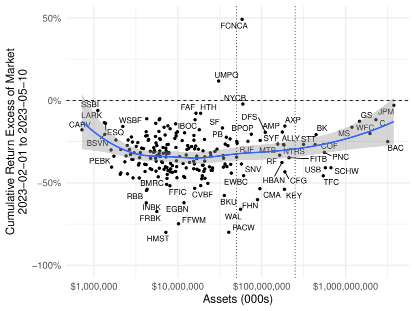
Notably, in Panel 3(d), we plot the same figure as 3(c) but exclude an outlier bank with a significant positive return. The shapes of the early and late return distributions in Panels 3(b) and 3(d) appear similar. However, the composition of these two distributions differs significantly. As indicated by the difference between the value-weighted return (in blue) and the equal-weighted return (in red), banks with large assets generally underperformed compared to small banks in 2022 (Panel 3(a)) and immediately after the SVB bank run (Panel 3(b)). Interestingly, this trend reversed in Panel 3(c), with the value-weighted returns significantly higher than the equal-weighted returns, indicating large banks outperforming small banks. We delve into the implications of these effects in Section 4.2.3.

(a) CAR since 2022-02-01

(b) CAR since 2023-02-01

(c) CAR since 2023-02-01

(d) CAR since 2023-02-01
Excluding FCNCA

Figure 3: Distribution of abnormal returns by time period. This figure plots the distribution of cumulative returns in excess of the S&P 500 index for the banks in our sample over three periods. In Panel (a), we report the distribution of cumulative returns as of January 31, 2023, measured since February 1, 2022. In Panel (b), we report the distribution of cumulative returns as of March 17, 2023, measured since February 1, 2023. In Panel (c), we report the distribution of cumulative returns as of May 17, 2023, measured since February 1, 2023. Panel (d) repeats Panel (c) excluding First Citizens Bankgroup. We additionally report the Dow Jones U.S. Bank Index cumulative return for each period as a vertical line, and the equal weighted mean of the banks in our sample for each period.

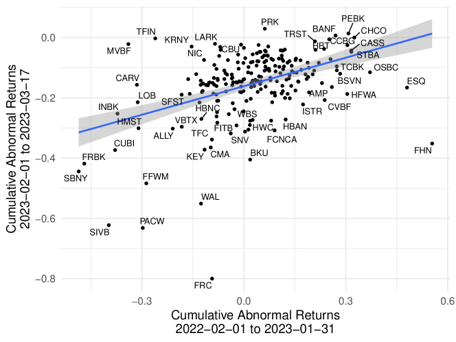
Lastly, we examine whether banks experiencing larger negative spillovers also demonstrated poorer performance in 2022. We do so by comparing cumulative returns before and immediately after the SVB bank run in Figure 4. Notably, there is a robust correlation between these two sets of returns across banks, with a bivariate $R^{2}$ of 0.18, and a regression coefficient of 0.31 with a corresponding $t$-statistic of 4.5. As the latter period captures the immediate negative spillovers associated with the SVB failure, this finding suggests that market participants, to some extent, anticipated and factored in the risks associated with the banking crisis of 2023 ahead of time.

Figure 4: 2022 bank excess returns vs 2023 bank excess returns. This figure compares cumulative returns in excess of the S&P 500 index for the banks in our sample for the 2022 period versus the early 2023 period. On the x-axis, we plot the cumulative returns in excess of the S&P 500 index for the banks in our sample from February 1, 2022 to January 31, 2023. On the y-axis, we plot the cumulative returns in excess of the S&P 500 index for the banks in our sample from February 1, 2023 to March 17, 2023. We also plot the least squares line of best fit. Stocks are denoted by their ticker symbol; Silicon Valley Bank’s ticker is SIVB.

4.2 Spillover effects – driving factors

We now examine the specific factors that explain the heterogeneous magnitudes of price declines resulting from the SVB failure. Models of bank runs suggest that a bank’s vulnerability is linked to various factors such as including asset quality, asset liquidity, funding outflow risk, and capitalization, among others.

We begin by discussing two vulnerabilities: uninsured deposits and unrealized losses on securities. Then, we explore whether other conventional factors such as asset liquidity, leverage, asset quality, or size are associated with the spillovers observed in this particular event. Finally, we discuss which of these vulnerabilities investors may have been anticipated, and which factors emerged as a “surprise” following the occurrence of the bank run.

4.2.1 Unique factors - uninsured deposits and unrealized losses on securities

As discussed in Section 2, the primary reason for the failure of SVB was concerns over unrealized losses in its security holdings, which prompted uninsured depositors to withdraw their funds. In normal circumstances, banks can use their liquid securities as buffers to alleviate shocks from funding outflows. However, with unrealized losses due to rate increases, liquidation of the HTM securities, while still “liquid”, would force banks to mark losses, exacerbating financial distress.

Deposits, even uninsured ones, typically serve as a reliable source of funding for banks as they are often considered less flighty than other market funding sources ([35, 34, 5]). Thanks to the deposit franchise, banks can also attract deposits at a lower cost than other sources ([9, 27, 28, 22, 23]). This conventional wisdom is also reflected in the liquidity regulation, where the LCR adopts relatively low run-off rates for deposit sources than other market funding ([6]).

However, during the 2023 crisis, banks could not easily exploit the deposit franchise as they needed to offer significant interest rates to attract or retain depositors ([38]). They also faced competition from other investment options, such as money market funds, which had access to the Fed’s reverse repo facility and were perceived as safe while offering high interest rates.

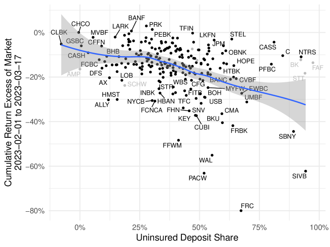
We begin by examining the link between banks’ reliance on uninsured deposits and negative stock returns in the aftermath of the SVB failure. As shown in Figure 5, which compares banks’ use of uninsured deposits to their stock performances, a clear negative relationship between the two can be observed. Notably, the three eventual failed banks - SVB, SBNY, and FRC - had exceptionally high uninsured deposit shares, with shares of 94%, 89%, and 67%, respectively, compared to the average share of 39%.

Figure 5: Cumulative returns vs. uninsured deposit share. This figure plots the cumulative returns in excess of the S&P 500 index for the banks in our sample from February 1, 2023 to March 17, 2023 against the uninsured deposit share (uninsured deposits as a share of total deposits) measured in 2022q4. See Section 3.1 for details on the data construction. The fitted line is a local linear regression (loess) curve. Stocks are denoted by their ticker symbol; Silicon Valley Bank’s ticker is SIVB.

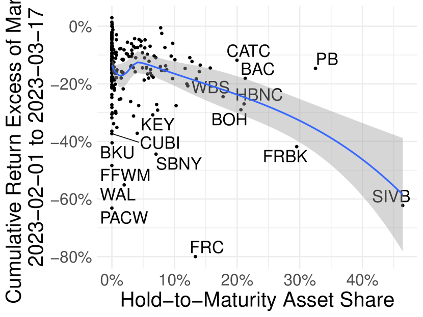
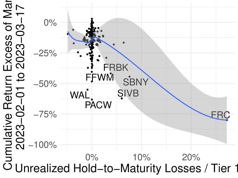
Next, we investigate the relationship between unrealized losses for HTM securities and negative stock returns. This relationship is plotted in Figure 6, which includes two panels. Panel A shows the ratio of a bank’s HTM securities to its total assets, while Panel B displays the ratio of a bank’s unrealized losses in HTM securities to its Tier 1 capital.

In Panel A, it can be seen that many banks have very small amounts of HTM securities, resulting in the HTM/asset shares being clustered around 0. However, there are several outliers with a large HTM/asset share, the most notable being SVB. Conditioning on larger shares of HTM, we observe a negative association between the shares of HTM securities and the stock returns.

In Panel B, unrealized HTM losses to Tier 1 capital are predominantly clustered around 0. This is due to many banks having minimal exposure to HTM securities, thereby constraining their potential losses. Additionally, certain banks may have opted for securities with lower duration risk compared to FRC or SVB. However, there is a negative association between the unrealized losses and the stock returns in the figure. It is worth noting that the implied losses from HTM securities, once recognized, would have reduced FRC’s Tier 1 capital by almost 30 percentage points.

(a) Hold-to-maturity asset share

(b) Unrealized HTM losses / Tier 1 Capital

Figure 6: Early cumulative returns explained by hold-to-maturity assets. Panel (a) plots the cumulative returns in excess of the S&P 500 index for the banks in our sample from February 1, 2023 to March 17, 2023 against the hold-to-maturity asset share (hold-to-maturity assets as a share of total assets) measured in 2022q4. Panel (b) plots against unrealized hold-to-maturity losses scaled by Tier 1 capital. See Section 3.1 for details on the data construction. The fitted lines are local linear regression (loess) curves. Stocks are denoted by their ticker symbol; Silicon Valley Bank’s ticker is SIVB.

We then estimate regressions of excess stock returns (i.e., 2023 early returns) on these bank characteristics. To ensure comparability, we standardize the control variables, which allows us to interpret the estimates as the changes in stock returns in response to a 1 standard deviation change in specific vulnerability factors. The results of these regressions are reported in Table 2.

Columns 1-3 of Table 2 represent linear regressions of excess cumulative returns on Uninsured Deposit Share, HTM Asset Share, and Unrealized HTM Losses/Tier 1 Capital. Notably, all estimates are statistically significant in explaining the negative excess returns. However, the estimate in column 3 for unrealized HTM losses is both statistically and economically the most significant.

In column 4, we include all three variables simultaneously. The results show that while the uninsured deposit share and unrealized HTM losses continue to predict negative excess returns, the actual HTM holdings do not. This finding aligns with earlier intuition, as investors would likely have greater concerns regarding the actual unrealized losses on HTM security portfolios rather than the holdings themselves. The estimates indicate that a one standard-deviation increase in unrealized HTM losses to Tier 1 capital (or uninsured deposit share) would lead to a 4.0 (or 2.7) percentage point lower excess stock returns.

Note that the presence of unrealized losses in banks’ HTM securities alone may not have a significant impact unless banks are compelled to sell these securities as a result of deposit outflows, say as a result of significant deposit outflows ([37]). This prediction is supported in column 5, where we include the interaction term between uninsured deposit shares and unrealized HTM losses. The estimate for the interaction term is negative and significant, while unrealized HTM losses by themselves are not significant.

Table 2: Cumulative returns correlated with uninsured deposits and HTM. This table reports estimated coefficients of regressions with the cumulative returns in excess of the S&P 500 index for the banks in our sample from February 1, 2023 to March 17, 2023 as the outcome. In Column (1), we report the bivariate relationship with the uninsured deposit share (uninsured deposts as a share of total deposits) measured in 2022q4. Column (2) reports the coefficient with the hold-to-maturity asset share (hold-to-maturity assets as a share of total assets) measured in 2022q4. Column (3) reports unrealized hold-to-maturity losses scaled by Tier 1 capital. Column (4) combines Columns (1)-(3). Column (5) adds the interaction of uninsured deposit share with HTM Asset Share and Unrealized HTM Losses. All variables (except for the cumulative returns) are mean zero and standarized to have standard deviation one, prior to interactions.

(1) (2) (3) (4) (5) (Intercept) -0.152^∗∗∗ -0.152^∗∗∗ -0.152^∗∗∗ -0.152^∗∗∗ -0.147^∗∗∗ (0.007) (0.007) (0.007) (0.006) (0.007) Uninsured Deposit Share -0.037^∗∗∗ -0.027^∗∗∗ -0.025^∗∗∗ (0.010) (0.008) (0.008) HTM Asset Share -0.033^∗∗∗ -0.012 -0.009 (0.011) (0.009) (0.007) Unrealized HTM Losses / Tier 1 Capital -0.050^∗∗∗ -0.040^∗∗∗ -0.011 (0.006) (0.006) (0.007) Uninsured Deposit Share $\times$ HTM Asset Share -0.001 (0.005) Uninsured Deposit Share $\times$ Unrealized HTM Losses / Tier 1 Capital -0.022^∗∗∗ (0.005) Observations 224 224 222 222 222 R² 0.112 0.089 0.198 0.273 0.302 Adjusted R² 0.108 0.085 0.195 0.263 0.286

4.2.2 What was the same this time and what differed?

The likelihood of depositors’ panic decreases when banks possess more liquid assets, more capital, or better-performing assets. Liquid assets, including cash and securities, can function as liquidity buffers to meet withdrawals, which helps to alleviate depositors’ concerns as well as losses from disorderly liquidations of illiquid assets ([6]). Higher capital buffers also mitigate depositors’ concerns by providing more loss absorption capacity. Furthermore, depositors have less reason to panic and withdraw when banks’ assets are safe and expected to generate greater future returns. We next investigate whether these factors contributed to the spillovers associated with the failure of SVB.

Liquid assets

We begin by examining the role of liquid assets, consisting of both cash and securities. We then analyze the effects of cash and securities separately to assess whether they had differential impacts.

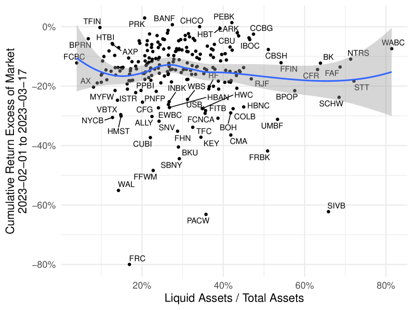
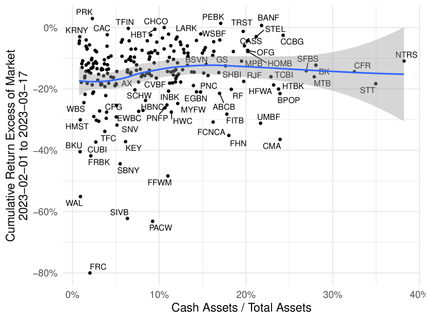
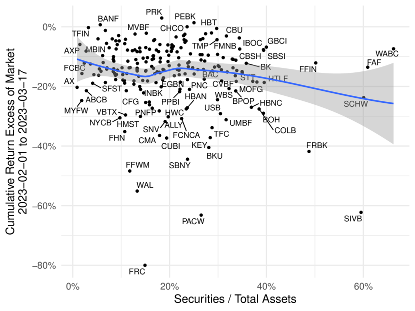
We report the linear regression estimates of these relationships in Table 3. In Column 1, the results indicate that overall holdings of liquid assets are not significantly associated with banks’ performance in response to the shock from the bank run, which differs from the typical implications. We see the corresponding graphical relationship in Panel A of Figure A1 in the Appendix. In fact, despite SVB holding more than 60% of its assets in cash and securities, it failed to withstand deposit withdrawals. Unlike typical bank run scenarios, depositor withdrawals exacerbated financial distress not through fire-sale losses of illiquid assets, but rather by realizing accounting losses on highly liquid securities that were marked as hold-to-maturity. This finding holds even when controlling for banks’ uninsured deposit reliance, as shown in column 3.

However, not all liquid assets yielded similar results. In Column 2, we find that higher cash holdings were indeed associated with a significant mitigation of the negative shock, whereas this was not the case with securities. HTM securities, despite being liquid, proved problematic in this specific episode as their liquidation would lead to the recognition of unrealized losses, thereby exacerbating the distress. We see the corresponding graphical relationship in Panel B and C of Figure A1.

The benefit of holding cash becomes more pronounced when we control for funding outflow risks by incorporating uninsured deposit shares in column 4. This results in a significant increase in the explanatory power (both for the estimate’s economic and statistically significance and $R^{2}$). The estimate indicates that a one-standard-deviation increase in cash to total assets would lead to a 2.7 percentage point increase in excess stock returns. In column 5, we additionally introduce an interaction term between cash (or securities) and uninsured deposit share. The estimate of the interaction term for cash is positive and significant, suggesting cash buffers effectively alleviate spillovers, particularly for banks facing higher funding outflow risks.

Table 3: Cumulative returns correlated with liquid assets. This table reports estimated coefficients of regressions with the cumulative returns in excess of the S&P 500 index for the banks in our sample from February 1, 2023 to March 17, 2023 as the outcome. In Column (1), we report the bivariate relationship with the liquid asset share (securities + cash scaled by total assets) measured in 2022q4. Column (2) adds uninsured deposit share to Column (1). Column (3) reports the coefficient with the cash scaled by total assets and securities scaled by total assets. Column (4) adds uninsured deposit share to Column (3). Column (5) interacts uninsured deposit share with cash and securities. All variables (except for the cumulative returns) are mean zero and standarized to have standard deviation one, prior to interactions.

(1) (2) (3) (4) (5) (Intercept) -0.152^∗∗∗ -0.152^∗∗∗ -0.152^∗∗∗ -0.152^∗∗∗ -0.153^∗∗∗ (0.007) (0.007) (0.007) (0.007) (0.007) Liquid Assets / Total Assets -0.005 0.008 (0.009) (0.009) Cash / Total Assets 0.014^∗∗ 0.027^∗∗∗ 0.022^∗∗∗ (0.007) (0.008) (0.007) Securities / Total Assets -0.014 -0.005 -0.003 (0.009) (0.008) (0.007) Uninsured Deposit Share -0.040^∗∗∗ -0.044^∗∗∗ -0.043^∗∗∗ (0.010) (0.010) (0.010) Cash / Total Assets $\times$ Uninsured Deposit Share 0.009^∗ (0.005) Securities / Total Assets $\times$ Uninsured Deposit Share -0.007 (0.010) Observations 224 224 224 224 224 R² 0.002 0.033 0.117 0.169 0.184 Adjusted R² -0.003 0.024 0.109 0.157 0.165

Capitalization

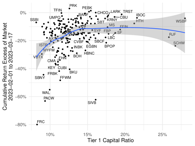
Next, we examine whether banks’ capitalization, as measured by the ratio of Tier 1 capital to risk-weighted assets (RWA), played a role in mitigating the spillover effects. As shown in Figure A2, we observe that, consistent with typical banking crises, better-capitalized banks exhibited relatively higher returns, especially among undercapitalized banks. It is worth noting that SVB does not appear to be specifically undercapitalized in this figure; but one should note that this capitalization measure does not account for the unrealized HTM losses.

We can confirm this relationship from the regression result reported in column 1 of Table 4, where a one-standard-deviation increase in the Tier 1 capital ratio is associated with a 3.0 percentage point increase in excess stock returns. The significance of capitalization in mitigating spillovers persists even when controlling for funding outflow risks, as shown in column 4, although the effect is less pronounced both statistically and economically. In column 5, we include the interaction terms to examine whether the stability effect of capitalization is more pronounced for banks facing higher funding outflow risks. While the coefficient for the interaction of capitalization and uninsured deposit shares is positive and sizable, its statistical significance is somewhat marginal, with a $t$-statistic of 1.6.

Table 4: Cumulative returns correlated with Tier 1 capital and non-performing loans. This table reports estimated coefficients of regressions with the cumulative returns in excess of the S&P 500 index for the banks in our sample from February 1, 2023 to March 17, 2023 as the outcome. In Column (1), we report the bivariate relationship with the non-performing loan ratio (non-performing loans scaled by total loans) measured in 2022q4. Column (2) reports the coefficient with the the Tier 1 capital ratio measured in 2022q4. Column (3) combines Column (1) and (2). Column (4) adds uninsured deposit share to Column (3). Column (5) interacts uninsured deposit share with non-performing loans and tier 1 capital. All variables (except for the cumulative returns) are mean zero and standarized to have standard deviation one, prior to interactions.

(1) (2) (3) (4) (5) (Intercept) -0.155^∗∗∗ -0.152^∗∗∗ -0.155^∗∗∗ -0.154^∗∗∗ -0.149^∗∗∗ (0.007) (0.007) (0.007) (0.007) (0.007) Tier 1 Capital Ratio 0.030^∗∗∗ 0.031^∗∗∗ 0.023^∗∗ 0.035^∗∗ (0.010) (0.010) (0.010) (0.014) Non-Performing Loans / Total Loans 0.0003 -0.001 -0.002 -0.005 (0.009) (0.009) (0.007) (0.007) Uninsured Deposit Share -0.034^∗∗∗ -0.037^∗∗∗ (0.010) (0.011) Tier 1 Capital Ratio $\times$ Uninsured Deposit Share 0.026 (0.016) Non-Performing Loans / Total Loans $\times$ Uninsured Deposit Share -0.003 (0.009) Observations 216 224 216 216 216 R² 0.074 $8.19\times 10^{-6}$ 0.074 0.156 0.201 Adjusted R² 0.070 -0.004 0.066 0.144 0.182

Asset quality

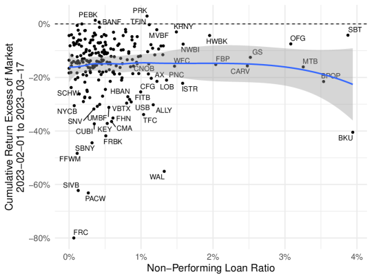
Finally, we examine whether asset quality, as measured by the non-performing loan (NPL) ratio, was associated with the contagion effect. In typical banking crises, concerns about bank asset quality, or “fundamentals,” amplify depositor panic and exacerbate bank runs ([41, 30]). However, in the case of the 2023 contagion, depositor panic was driven by implied losses from duration mismatch rather than credit risks. As illustrated in Figure A3, there was no discernible effect of better-performing assets in mitigating the negative spillovers. Moreover, the regression estimates in Table 4 indicate that the NPL ratio was not a statistically significant predictor in all of the specifications.

In sum, asset liquidity in general or better-performing assets did not help mitigate the spillovers during the bank runs of 2023. Securities like Treasury or government-sponsored enterprise (GSE) bonds, while liquid, did not reduce bank stress because their liquidations would result in realizations of implied losses. Cash and capital, on the other hand, were still effective in reducing the stress. It was uninsured deposits that became problematic, in combination with the implied losses in the HTM securities portfolio.

4.2.3 Did size matter? Immediate vs. medium-term effects

(a) Early cumulative returns

(b) Late cumulative returns

Figure 7: Cumulative returns explained by total assets. Panel (a) of this figure plots the cumulative returns in excess of the S&P 500 index for the banks in our sample from February 1, 2023 to March 17, 2023 against the assets measured in 2022q4. Panel (b) of this figure plots the cumulative returns in excess of the S&P 500 index for the banks in our sample from February 1, 2023 to May 10, 2023 against the assets measured in 2022q4. See Section 3.1 for details on the data construction. The fitted lines are local linear regression (loess) curves. Stocks are denoted by their ticker symbol; Silicon Valley Bank’s ticker is SIVB.

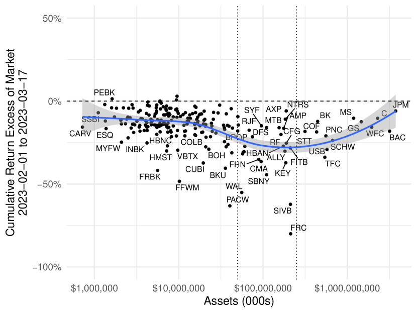
Next, we investigate whether bank size was associated with negative returns. Figure 7(a) displays the “early” cumulative returns plotted against bank assets. The figure suggests the presence of differential spillover effects across different asset size categories. A notable observation is the heightened stress experienced by mid-sized banks, particularly super-regional banks falling between assets of $50 billion and $250 billion, denoted by the two vertical lines. As discussed in Section 2, these banks, including SVB, were initially designated as systemically important following the regulatory reforms implemented after the financial crisis, but faced relaxed regulations with the regulatory rollback in 2019. One possible interpretation is that investors exhibited greater concerns with banks of a similar size to SVB, particularly in the aftermath of its failure.

Table 5: Cumulative returns correlated with asset size. This table reports estimated coefficients of regressions with the cumulative returns in excess of the S&P 500 index for the banks in our sample. In Column (1), we report the relationship with binned indicator variables of total assets measured in 2022q4. The bins exhaustively bin out all observations, and do not include a constant, so each coefficient is the average for each bin. Column (2) includes the binned controls for assets (excluding the bin for banks with total assets less than 5 billion dollars) and a constant, as well as the controls for uninsured deposit share, Tier 1 capital ratio, cash/total assets and unrealized hold-to-maturity losses. Column 3 adds the cumulative abnormal return from February 1, 2022 to January 31, 2023 to Column (2). Columns (1)-(3) use cumluative returns from February 1, 2023 to March 17, 2023 as the outcome. Columns (4)-(6) repeat Columns (1)-(3) and use cumluative returns from February 1, 2023 to May 10, 2023 as the outcome. All variables (except for the cumulative returns) are mean zero and standarized to have standard deviation one, prior to interactions.

(1) (2) (3) (4) (5) (6) Assets [0-5b] -0.113^∗∗∗ -0.319^∗∗∗ (0.009) (0.016) Assets (5b-10b] -0.115^∗∗∗ 0.002 0.008 -0.331^∗∗∗ 0.0005 0.008 (0.010) (0.013) (0.011) (0.015) (0.022) (0.021) Assets (10b-50b] -0.160^∗∗∗ -0.041^∗∗∗ -0.041^∗∗∗ -0.354^∗∗∗ -0.014 -0.015 (0.013) (0.016) (0.013) (0.017) (0.025) (0.022) Assets (50b-250b] -0.283^∗∗∗ -0.147^∗∗∗ -0.132^∗∗∗ -0.375^∗∗∗ -0.019 0.0009 (0.032) (0.022) (0.023) (0.060) (0.048) (0.050) Assets (250b-1tr] -0.224^∗∗∗ -0.115^∗∗∗ -0.096^∗∗∗ -0.333^∗∗∗ 0.011 0.036 (0.026) (0.027) (0.027) (0.033) (0.045) (0.045) Assets (1tr-10tr] -0.122^∗∗∗ 0.003 0.011 -0.148^∗∗∗ 0.211^∗∗∗ 0.223^∗∗∗ (0.016) (0.022) (0.022) (0.029) (0.045) (0.044) (Intercept) -0.122^∗∗∗ -0.132^∗∗∗ -0.338^∗∗∗ -0.352^∗∗∗ (0.009) (0.008) (0.018) (0.017) Uninsured Deposit Share -0.023^∗∗∗ -0.014^∗∗ -0.066^∗∗∗ -0.053^∗∗∗ (0.008) (0.007) (0.014) (0.012) Tier 1 Capital Ratio 0.014^∗∗ 0.015^∗∗ 0.009 0.010 (0.006) (0.006) (0.011) (0.011) Cash / Total Assets 0.028^∗∗∗ 0.017^∗∗ 0.054^∗∗∗ 0.039^∗∗∗ (0.007) (0.007) (0.011) (0.010) Unrealized HTM Losses / Tier 1 Capital -0.034^∗∗∗ -0.032^∗∗∗ -0.036^∗∗∗ -0.034^∗∗∗ (0.004) (0.005) (0.007) (0.007) Cumulative Abnormal Returns (2022) 0.220^∗∗∗ 0.288^∗∗∗ (0.057) (0.095) Observations 224 216 216 224 216 216 R² 0.241 0.492 0.566 0.045 0.349 0.408 Adjusted R² 0.224 0.470 0.545 0.023 0.321 0.380

The regression estimates presented in Table 5 provide further confirmation of the particular stress experienced by these regional banks with similar size immediately after the SVB failure. In Column 1, dummy variables are included for each of the six size buckets, where each estimate indicates the average excess returns for that specific size group relative to the market returns. For only this column, we exclude the constant, so each coefficient should represents the average return in the size bucket. Column 2 incorporates the bank characteristics (i.e., vulnerability factors) that we identified as being associated with the spillovers, including uninsured deposit share, capitalization, cash holdings, and unrealized HTM security losses. Additionally, a constant term is included and we exclude the size indicator variable for the smallest asset size group, implying that the estimates for the asset groups reflect excess returns relative to banks with less than 5 billion dollars in assets.

The estimates in column 2 highlight the significant stress experienced by regional banks. When compared to banks with assets below $5 billion, banks within the size range of $10 billion and $1 trillion had significant additional negative returns, with the most pronounced effect observed among banks between $50 billion and $250 billion, exhibiting returns that were 15 percentage points lower. The estimates indicate that unrealized losses were the most economically significant predictors of the scale of spillover effects immediately after the SVB failure, followed by cash, uninsured deposits, and capitalization.

Differential medium-term effect The size effect, however, presents a different pattern over time. Figure 7(b) displays banks’ “late” returns two months after the SVB failure, from February 1, 2023 to May 10, 2023. Unlike the immediate effect shown in Figure 7(a), the substantial negative impact had spread beyond mid-sized banks in the $50 billion and $250 billion range to include smaller banks as well.

The regression estimates reported in columns 4 to 6 of Table 5 repeats the exercise from column 1 through 3 for the late returns. The banking sector, as a whole, experienced a further decline in stock prices over time (column 4) compared to immediately after the SVB failure (column 1), with the most significant decrease observed for banks below $50 billion in assets. While policy measures, such as the FDIC’s full protection of failed bank deposits and the Federal Reserve’s new lending facility, helped prevent additional bank runs, concerns about the soundness of the entire banking system spread. This is potentially because the fundamental driver of banking stress was the unrealized losses in banks’ long-term assets, which included not only HTM securities but also fixed-rate mortgage loans, which affected a broad range of banks. The absence of any indication of a rate cut by the central bank further heightened these concerns, resulting in stress for the entire banking sector.

However, amidst broader stress, we can observe the distinct outperformance of very large banks compared to the rest of the system. Column 5 suggests that banks with assets greater than $1 trillion had higher returns by 21 percentage points than other banks, while none of the other size groups performed differently. This trend aligns with the earlier observations of equal-weighted and value-weighted returns.

Why did investors treat these largest banks differently during a period of systemic stress? While it is evident that these banks were subject to more robust regulation and supervision than smaller banks, including SVB, and thus were likely in better financial health, this regulatory difference alone does not fully explain the positive association between size and return among them. While banks larger than $250 billion were also designated as “systemically important” to face the tougher regulations, they did not outperform the rest – only those larger than $1 trillion did so.

One possible explanation for this pattern is the implicit guarantees associated with too-big-to-fail (TBTF) banks. Even among the similarly regulated SIFIs larger than $250 billion in assets, investors seemed to have priced in greater TBTF benefits for the largest banks. In fact, being perceived as safe, these banks also experienced deposit inflows amid a flight to quality by depositors, which further helped them mitigate the system-wide stress ([11]). Those with deposit outflows, on the other hand, were forced to resort to more expensive funding sources, such as time deposits and borrowing from the Federal Reserve or Federal Home Loan Banks ([38]).

4.3 What was expected by the market and what was a surprise?

Having established the factors associated with the spillovers, our next focus is to examine whether market participants had anticipated these vulnerabilities in advance or if they were caught by surprise following the SVB bank run. As discussed in Section 4.1, there was a strong association between banks’ stock returns in 2022 and those immediately after the SVB bank run, indicating investors had expectations of vulnerabilities before the run occurred.

Indeed, in columns 3 and 6 of Table 5, we observe that risks associated with uninsured deposit reliance or cash holdings were partly anticipated by investors, as indicated by their diminished significance both statistically and economically when controlling for the 2022 returns. However, the inclusion of the lagged returns has little effect on the explanatory power of size, HTM losses, or capitalization, indicating that investors were potentially surprised by these factors, leading to additional negative returns in response to the SVB bank run.

To further explore this, we evaluate the correlation between each bank’s stock return prior to the 2023 crisis (i.e., “2022 returns” from 2022-02-01 to 2023-01-31) and their vulnerability characteristics. A stronger correlation would indicate that investors had more pronounced concerns regarding specific vulnerabilities. Note that we hold these vulnerability factors fixed to the observed measures from the 2022q4 filings.

In Table 6, we regress banks’ 2022 returns on the respective vulnerability factors we have previously assessed. Focusing on the factors we identified to be relevant, our results indicate that market investors to some degree accounted for possible losses associated with heavy reliance on uninsured deposits and limited cash holdings, as evidenced by their significant correlation with the 2022 returns. These losses could result from increases in funding costs or deposit outflows in the face of central bank tightening. Furthermore, the inclusion of these factors as regression controls leads to a distinct increase in the $R^{2}$ value. Notably, the vulnerabilities associated with asset size, HTM unrealized losses, and capitalization did not appear to be reflected in the 2022 returns. This indicates that investors considered the recognition of implied securities loss, which would materialize if banks were forced to sell these securities, to be unlikely.

Table 6: Cumulative returns in 2022 correlated with vulnerability factors. This table reports estimated coefficients of regressions with the cumulative returns in excess of the S&P 500 index for the banks in our sample from February 1, 2022 to January 31, 2023. In Column (1), we report the relationship with binned indicator variables of total assets measured in 2022q4. The bins exhaustively bin out all observations, and do not include a constant, so each coefficient is the average for each bin. Column (2) includes the binned controls for assets (excluding the bin for banks with total assets less than 5 billion dollars) and a constant, as well as the controls for uninsured deposit share, hold-to-maturity asset share, and unrealized hold-to-maturity losses. Column (3) includes cash/total assets and securities/total assets. Column (4) includes Tier 1 capital ratio and non-performing loan ratio. All variables are mean zero and standarized to have standard deviation one, prior to interactions.

(1) (2) (3) (4) Assets [0-5b] 0.050^∗∗ (0.024) Assets (5b-10b] 0.023 -0.025 -0.017 -0.025 (0.019) (0.031) (0.030) (0.029) Assets (10b-50b] 0.043^∗∗∗ 0.005 0.010 0.005 (0.015) (0.029) (0.029) (0.029) Assets (50b-250b] -0.006 -0.039 -0.060 -0.060 (0.037) (0.042) (0.041) (0.041) Assets (250b-1tr] -0.038^∗ -0.061 -0.085^∗∗ -0.084^∗∗ (0.022) (0.043) (0.038) (0.038) Assets (1tr-10tr] 0.005 -0.008 -0.033 -0.018 (0.038) (0.045) (0.041) (0.046) (Intercept) 0.041 0.040 0.046^∗ (0.025) (0.025) (0.024) Uninsured Deposit Share -0.021^∗ -0.034^∗∗∗ -0.042^∗∗∗ (0.012) (0.012) (0.013) HTM Asset Share -0.007 -0.005 -0.006 (0.015) (0.013) (0.013) Unrealized HTM Losses / Tier 1 Capital -0.012 -0.007 -0.007 (0.011) (0.012) (0.011) Cash / Total Assets 0.048^∗∗∗ 0.052^∗∗∗ (0.010) (0.011) Securities / Total Assets -0.0005 -0.0002 (0.010) (0.011) Tier 1 Capital Ratio -0.003 (0.012) Non-Performing Loans / Total Loans -0.014 (0.010) Observations 224 222 222 216 R² 0.016 0.058 0.145 0.175 Adjusted R² -0.007 0.023 0.104 0.127

How can we interpret these null results when all relevant information was publicly available? The information view of banking panics (see, e.g., [31], [18]) can provide a plausible framework. The view argues that abrupt shifts in depositors’ risk perception of bank assets, triggered by the arrival of negative news such as a failure of a large institution or adverse macroeconomic perspectives, can cause widespread bank runs.

Even though the presence of unrealized losses in banks’ securities portfolios affects their fundamentals, this vulnerability would only materialize when banks were forced to liquidate these assets to generate cash in the face of severe deposit outflows. Hence, unless depositors are concerned about these implied losses, stock investors have little reason to pay close attention to them, either. While investors did take into account the possible negative impacts associated with uninsured deposit reliance, they at least did not anticipate the implied losses to be the driving factor of severe deposit outflows. The SVB episode, however, potentially caused a significant shift in this dynamic through depositors’ risk perceptions.

A similar speculative argument can be made for bank size. While the size of a bank can influence its likelihood of survival, this factor becomes critical particularly when experiencing systemic instability. Following the SVB failure, investors became aware of the vulnerability faced by mid-sized banks and the relaxation of regulations that they experienced. As concerns about the entire banking system grew over time, flying-to-quality investors sought safety in the largest “systemic” banks. However, these effects are significant only when conditioned on the occurrence of a systemic disruption, which may have a small unconditional probability ex ante. It is worth noting that the U.S. banking system was generally perceived to be well-capitalized before the 2023 crisis, which may explain the limited association between bank capitalization and 2022 returns.

It is important to note that lack of information was not a constraint. The bank balance sheet information (including unrealized losses) had been announced for 2022Q4 by the end of January 2023, and the accumulated HTM losses had been apparent prior to Q4 as well. Hence, there was no sense of hidden information on implied losses. Rather, the SVB bank run seems to have served as a device to change investors’ risk perceptions to cause widespread spillovers.

5 Conclusion

This paper analyzes the SVB bank failure, focusing on the bank balance sheet factors associated with contagion on the rest of the banking system.

Lessons from the GFC suggested that liquidity risks could be managed by holding liquid assets, including cash and “high-quality” securities, or funding with more deposits than wholesale funding. However, the recent SVB failure episode showed that these measures may not always help prevent bank runs. The panic was triggered by concerns about unrealized losses in their HTM securities portfolio, albeit of high-quality, which led uninsured depositors to panic. This forced the banks to sell their HTM securities, resulting in the realization of implied losses, exacerbating the run.

Furthermore, it is worth noting that, in this particular case, cash and liquid securities were not interchangeable in reducing damages from deposit outflows. While some banks had adequate HQLAs from the standpoint of the regulatory requirements such as LCR, interest rate risks caused significant losses even on sufficiently liquid securities. These securities did not effectively serve as liquidity buffers against funding outflows; only cash and capital buffers were successful in absorbing losses and containing the spillovers.

We also find that banks whose stocks experienced more negative returns following the failure of SVB had already underperformed in the previous year. Our finding suggests that investors, to some extent, anticipated the downsides associated with uninsured deposit reliance during the rate hikes. However, they did not foresee the damages associated with unrealized securities losses until the SVB run, even though the data was widely available. This highlights the challenges in devising comprehensive and robust stress scenarios.

In many respects, the SVB episode highlights new channels for bank failures and contagion, providing us with novel lessons. Some of the elegantly designed measures based on the experiences of the GFC did not effectively prevent the systemic instability this time. A major driver for the spillovers was implied losses in the banks’ securities portfolio, but this was not adequately considered in either the regulatory stress test scenarios or the investors’ risk pricing ex ante. Moreover, the treatment and incorporation of these implied losses into regulatory measures would pose important challenges as such losses crystallize only when banks are forced to sell held-to-maturity assets at market prices. These are important topics for further research and, going forward, policymakers should incorporate these lessons into their policies to enhance the resilience of the financial system.

(a) Liquid/ Assets

(b) Cash/ Assets

(c) Securities/ Assets

Figure A1: Early cumulative returns explained by liquid assets. Panel (a) plots the cumulative returns in excess of the S&P 500 index for the banks in our sample from February 1, 2023 to March 17, 2023 against the liquid asset share (sum of liquid securities and cash scaled by total assets) measured in 2022q4. Panel (b) plots against cash scaled by total assets. Panel (c) plots against liquid securities scaled by total assets. See Section 3.1 for details on the data construction. The fitted lines are local linear regression (loess) curves. Stocks are denoted by their ticker symbol; Silicon Valley Bank’s ticker is SIVB.

Figure A2: Early cumulative returns explained by Tier 1 Capital ratio. This figure plots the cumulative returns in excess of the S&P 500 index for the banks in our sample from February 1, 2023 to March 17, 2023 against the Tier 1 capital ratio measured in 2022q4. See Section 3.1 for details on the data construction. The fitted line is a local linear regression (loess) curve. Stocks are denoted by their ticker symbol; Silicon Valley Bank’s ticker is SIVB.

Figure A3: Early cumulative returns explained by non-performing loan ratio. This figure plots the cumulative returns in excess of the S&P 500 index for the banks in our sample from February 1, 2023 to March 17, 2023 against the non-performing loan ratio (non-performing loans scaled by total loans) measured in 2022q4. See Section 3.1 for details on the data construction. The fitted line is a local linear regression (loess) curve. Stocks are denoted by their ticker symbol; Silicon Valley Bank’s ticker is SIVB.

Table A1: Cumulative returns correlated with uninsured deposits and HTM. This table reports estimated coefficients of regressions with the cumulative returns in excess of the S&P 500 index for the banks in our sample from February 1, 2023 to May 10, 2023 as the outcome. In Column (1), we report the bivariate relationship with the uninsured deposit share (uninsured deposts as a share of total deposits) measured in 2022q4. Column (2) reports the coefficient with the hold-to-maturity asset share (hold-to-maturity assets as a share of total assets) measured in 2022q4. Column (3) reports unrealized hold-to-maturity losses scaled by Tier 1 capital. Column (4) combines Columns (1)-(3). Column (5) adds the interaction of uninsured deposit share with HTM Asset Share and Unrealized HTM Losses. All variables (except for the cumulative returns) are mean zero and standarized to have standard deviation one, prior to interactions.

(1) (2) (3) (4) (5) (Intercept) -0.336^∗∗∗ -0.336^∗∗∗ -0.338^∗∗∗ -0.338^∗∗∗ -0.325^∗∗∗ (0.010) (0.011) (0.010) (0.010) (0.010) Uninsured Deposit Share -0.051^∗∗∗ -0.044^∗∗∗ -0.040^∗∗∗ (0.016) (0.013) (0.011) HTM Asset Share -0.037^∗∗ -0.010 -0.005 (0.018) (0.015) (0.012) Unrealized HTM Losses / Tier 1 Capital -0.052^∗∗∗ -0.039^∗∗∗ 0.036^∗∗ (0.012) (0.011) (0.015) Uninsured Deposit Share $\times$ HTM Asset Share 0.0004 (0.008) Uninsured Deposit Share $\times$ Unrealized HTM Losses / Tier 1 Capital -0.057^∗∗∗ (0.011) Observations 224 224 222 222 222 R² 0.097 0.052 0.102 0.181 0.268 Adjusted R² 0.093 0.048 0.098 0.170 0.251

Table A2: Cumulative returns correlated with liquid assets. This table reports estimated coefficients of regressions with the cumulative returns in excess of the S&P 500 index for the banks in our sample from February 1, 2023 to March 17, 2023 as the outcome. In Column (1), we report the bivariate relationship with the liquid asset share (securities + cash scaled by total assets) measured in 2022q4. Column (2) adds uninsured deposit share to Column (1). Column (3) reports the coefficient with the cash scaled by total assets and securities scaled by total assets. Column (4) adds uninsured deposit share to Column (3). Column (5) interacts uninsured deposit share with cash and securities. All variables (except for the cumulative returns) are mean zero and standarized to have standard deviation one, prior to interactions.

(1) (2) (3) (4) (5) (Intercept) -0.336^∗∗∗ -0.336^∗∗∗ -0.336^∗∗∗ -0.336^∗∗∗ -0.339^∗∗∗ (0.011) (0.011) (0.010) (0.010) (0.010) Liquid Assets / Total Assets 0.008 0.027^∗∗ (0.013) (0.012) Cash / Total Assets 0.039^∗∗∗ 0.059^∗∗∗ 0.053^∗∗∗ (0.009) (0.010) (0.011) Securities / Total Assets -0.014 0.0001 -0.002 (0.013) (0.012) (0.009) Uninsured Deposit Share -0.059^∗∗∗ -0.068^∗∗∗ -0.070^∗∗∗ (0.015) (0.015) (0.013) Cash / Total Assets $\times$ Uninsured Deposit Share 0.009 (0.008) Securities / Total Assets $\times$ Uninsured Deposit Share 0.003 (0.017) Observations 224 224 224 224 224 R² 0.002 0.068 0.122 0.218 0.224 Adjusted R² -0.002 0.059 0.114 0.207 0.206

Table A3: Cumulative returns correlated with Tier 1 capital and non-performing loans. This table reports estimated coefficients of regressions with the cumulative returns in excess of the S&P 500 index for the banks in our sample from February 1, 2023 to May 10, 2023 as the outcome. In Column (1), we report the bivariate relationship with the non-performing loan ratio (non-performing loans scaled by total loans) measured in 2022q4. Column (2) reports the coefficient with the the Tier 1 capital ratio measured in 2022q4. Column (3) combines Column (1) and (2). Column (4) adds uninsured deposit share to Column (3). Column (5) interacts uninsured deposit share with non-performing loans and tier 1 capital. All variables (except for the cumulative returns) are mean zero and standarized to have standard deviation one, prior to interactions.

(1) (2) (3) (4) (5) (Intercept) -0.338^∗∗∗ -0.336^∗∗∗ -0.339^∗∗∗ -0.338^∗∗∗ -0.330^∗∗∗ (0.011) (0.011) (0.011) (0.010) (0.011) Tier 1 Capital Ratio 0.045^∗∗∗ 0.044^∗∗∗ 0.034^∗∗∗ 0.049^∗∗∗ (0.012) (0.012) (0.012) (0.018) Non-Performing Loans / Total Loans 0.019^∗ 0.017 0.016 0.012 (0.011) (0.011) (0.010) (0.009) Uninsured Deposit Share -0.049^∗∗∗ -0.051^∗∗∗ (0.017) (0.016) Tier 1 Capital Ratio $\times$ Uninsured Deposit Share 0.036^∗ (0.020) Non-Performing Loans / Total Loans $\times$ Uninsured Deposit Share 0.003 (0.013) Observations 216 224 216 216 216 R² 0.076 0.014 0.087 0.165 0.204 Adjusted R² 0.071 0.009 0.078 0.153 0.185

References

- [1] Viral V Acharya and Tanju Yorulmazer “Information contagion and bank herding” In Journal of Money, Credit and Banking 40.1 Wiley Online Library, 2008, pp. 215–231
- [2] Viral V. Acharya et al. “SVB and Beyond: The Banking Stress of 2023”, 2023 DOI: 10.2139/ssrn.4513276
- [3] Franklin Allen and Douglas Gale “Optimal Financial Crises” In Journal of Finance 53.4 Blackwell Publishers Inc., 1998, pp. 1245–1284
- [4] Franklin Allen and Douglas Gale “Financial Contagion” In Journal of Political Economy 108.1 The University of Chicago Press, 2000, pp. 1–33
- [5] Jennie Bai, Arvind Krishnamurthy and Charles-Henri Weymuller “Measuring Liquidity Mismatch in the Banking Sector” In Journal of Finance 73.1 Wiley Online Library, 2018, pp. 51–93
- [6] BCBS “Basel III: The liquidity coverage ratio and liquidity risk monitoring tools” Bank for International Settlements, 2013
- [7] Juliane Begenau, Monika Piazzesi and Martin Schneider “Banks’ Risk Exposures”, Working Paper Series 21334, 2015 DOI: 10.3386/w21334
- [8] Efraim Benmelech, Jun Yang and Michal Zator “Bank Branch Density and Bank Runs”, 2023
- [9] Allen N. Berger, Gerald A. Hanweck and David B. Humphrey “Competitive viability in banking: Scale, scope, and product mix economies” In Journal of Monetary Economics 20.3, 1987, pp. 501–520 DOI: https://doi.org/10.1016/0304-3932(87)90039-0
- [10] Arnoud WA Boot, Todd T Milbourn and Anjolein Schmeits “Credit ratings as coordination mechanisms” In The Review of Financial Studies 19.1 Oxford University Press, 2006, pp. 81–118
- [11] Cecilia Caglio, Jennifer Dlugosz and Marcelo Rezende “Flight to Safety in the Regional Bank Crisis of 2023” In Available at SSRN 4457140, 2023
- [12] Charles W Calomiris and Gary Gorton “The origins of banking panics: models, facts, and bank regulation” In Financial Markets and Financial Crises University of Chicago Press, 1991, pp. 109–174
- [13] Charles W. Calomiris and Charles M. Kahn “The Role of Demandable Debt in Structuring Optimal Banking Arrangements” In American Economic Review 81.3 American Economic Association, 1991, pp. 497–513
- [14] Varadarajan V Chari and Ravi Jagannathan “Banking panics, information, and rational expectations equilibrium” In Journal of Finance 43.3 Wiley Online Library, 1988, pp. 749–761
- [15] Yehning Chen “Banking panics: The role of the first-come, first-served rule and information externalities” In Journal of Political Economy 107.5 The University of Chicago Press, 1999, pp. 946–968
- [16] Rodrigo Cifuentes, Gianluigi Ferrucci and Hyun Song Shin “Liquidity risk and contagion” In Journal of the European Economic Association 3.2-3 Oxford University Press, 2005, pp. 556–566
- [17] J Anthony Cookson et al. “Social Media as a Bank Run Catalyst” In Available at SSRN 4422754, 2023
- [18] Tri Vi Dang, Gary Gorton and Bengt Holmström “The information view of financial crises” In Annual Review of Financial Economics 12 Annual Reviews, 2020, pp. 39–65
- [19] Francesco D’Ercole and Alexander F Wagner “The green energy transition and the 2023 Banking Crisis” In Finance Research Letters Elsevier, 2023, pp. 104493
- [20] Douglas W. Diamond and Philip H. Dybvig “Bank Runs, Deposit Insurance, and Liquidity” In Journal of Political Economy 91.3 The University of Chicago Press, 1983, pp. 401–419
- [21] Douglas W. Diamond and Raghuram G. Rajan “Liquidity Risk, Liquidity Creation, and Financial Fragility: A Theory of Banking” In Journal of Political Economy 109.2 The University of Chicago Press, 2001, pp. 287–327
- [22] Itamar Drechsler, Alexi Savov and Philipp Schnabl “The deposits channel of monetary policy” In Quarterly Journal of Economics 132.4 Oxford University Press, 2017, pp. 1819–1876
- [23] Itamar Drechsler, Alexi Savov and Philipp Schnabl “Banking on deposits: Maturity transformation without interest rate risk” In Journal of Finance 76.3 Wiley Online Library, 2021, pp. 1091–1143
- [24] Itamar Drechsler et al. “Banking on Uninsured Deposits”, Working Paper Series 31138, 2023 DOI: 10.3386/w31138
- [25] Thomas M. Eisenbach et al. “Stability of Funding Models: An Analytical Framework” In Federal Reserve Bank of New York Economic Policy Review 20.1, 2014, pp. 29–49
- [26] Mark J Flannery and Sorin M Sorescu “Partial Effects of Fed Tightening on US Banks’ Capital” In Available at SSRN 4424139, 2023
- [27] D. Gale and T. Yorulmazer “Bank capital, fire sales, and the social value of deposits” In Econ Theory 69 Springer, 2020, pp. 919–963 DOI: 10.1007/s00199-019-01189-5
- [28] Evan Gatev and Philip E Strahan “Banks’ advantage in hedging liquidity risk: Theory and evidence from the commercial paper market” In Journal of Finance 61.2 Wiley Online Library, 2006, pp. 867–892
- [29] Paul Goldsmith-Pinkham and Tanju Yorulmazer “Liquidity, bank runs, and bailouts: spillover effects during the Northern Rock episode” In Journal of Financial Services Research 37 Springer, 2010, pp. 83–98
- [30] Itay Goldstein and Ady Pauzner “Demand–deposit contracts and the probability of bank runs” In Journal of Finance 60.3 Wiley Online Library, 2005, pp. 1293–1327
- [31] Gary Gorton “Banking panics and business cycles” In Oxford Economic Papers 40.4 Oxford University Press, 1988, pp. 751–781
- [32] Gary Gorton and Lixin Huang “Liquidity, efficiency, and bank bailouts” In American Economic Review 94.3 American Economic Association, 2004, pp. 455–483
- [33] Valentin Haddad, Barney Hartman-Glaser and Tyler Muir “Bank Fragility When Depositors Are the Asset” In Available at SSRN 4412256, 2023
- [34] Samuel G Hanson et al. “Banks as patient fixed-income investors” In Journal of Financial Economics 117.3 Elsevier, 2015, pp. 449–469
- [35] Victoria Ivashina and David Scharfstein “Bank lending during the financial crisis of 2008” In Journal of Financial Economics 97.3 Elsevier, 2010, pp. 319–338
- [36] Erica Xuewei Jiang et al. “Limited Hedging and Gambling for Resurrection by US Banks During the 2022 Monetary Tightening?” In Available at SSRN, 2023
- [37] Erica Xuewei Jiang et al. “Monetary Tightening and U.S. Bank Fragility in 2023: Mark-to-Market Losses and Uninsured Depositor Runs?”, Working Paper Series 31048, 2023 DOI: 10.3386/w31048
- [38] Alena Kang-Landsberg, Stephan Luck and Matthew Plosser “Deposit Betas: Up, Up, and Away?” In Liberty Street Economics, 2023 URL: https://libertystreeteconomics.newyorkfed.org/2023/04/deposit-betas-up-up-and-away/
- [39] Stephan Luck, Matthew Plosser and Josh Younger “Bank Funding during the Current Monetary Policy Tightening Cycle” In Liberty Street Economics, 2023 URL: https://libertystreeteconomics.newyorkfed.org/2023/05/bank-funding-during-the-current-monetary-policy-tightening-cycle/
- [40] Bill Nelson “Silicon Valley Bank Would Have Passed The Liquidity Coverage Ratio Requirement” In Bank Policy Institute blog, 2023 URL: https://bpi.com/silicon-valley-bank-would-have-passed-the-liquidity-coverage-ratio-requirement/
- [41] Jean-Charles Rochet and Xavier Vives “Coordination failures and the lender of last resort: was Bagehot right after all?” In Journal of the European Economic Association 2.6 Oxford University Press, 2004, pp. 1116–1147