DCNFIS: Deep Convolutional Neuro-Fuzzy Inference System

Abstract

A key challenge in eXplainable Artificial Intelligence is the well-known tradeoff between the transparency of an algorithm (i.e., how easily a human can directly understand the algorithm, as opposed to receiving a post-hoc explanation), and its accuracy. We report on the design of a new deep network that achieves improved transparency without sacrificing accuracy. We design a deep convolutional neuro-fuzzy inference system (DCNFIS) by hybridizing fuzzy logic and deep learning models and show that DCNFIS performs as accurately as three existing convolutional neural networks on four well-known datasets. We furthermore that DCNFIS outperforms state-of-the-art deep fuzzy systems. We then exploit the transparency of fuzzy logic by deriving explanations, in the form of saliency maps, from the fuzzy rules encoded in DCNFIS. We investigate the properties of these explanations in greater depth using the Fashion-MNIST dataset.

I Introduction

Deep Neural Networks (DNNs) are the heart of the “new” Artificial Intelligence (AI) (as exemplified by AlphaGo’s defeat of a human champion). DNNs are currently the most accurate solutions for many problems, including image recognition [1], Natural Language Processing (NLP) [2], speech recognition [3], robotic surgery [4], medical diagnosis [5] and many others. However, knowledge in a DNN is encoded as a distributed pattern of potentially hundreds of billions of connection weights [6]. This is an incomprehensible reresentation for human beings. Add to this the fact that some of their decisions seem counter-intuitive or even inexplicable to human experts, and it seems likely that humans would be reluctant to trust a DNN. Indeed, the literature bears this out [7, 8, 9]. There is a risk that, far from embracing the AI revolution, human society might reject it if new mechanisms to foster trust in AI are not developed.

A classical approach to the interpretability problem is to incorporate an “explanation mechanism” in AI algorithms [10, 7, 8, 9]; such approaches have recently been dubbed eXplainable Artificial Intelligence (XAI). Explanations in turn enable knowledge discovery [11], algorithm verifiability [12], and even legal compliance (by satisfying the ”right to an explanation” that increasingly appears in privacy protection legislation) [13]. A discussion of the history of XAI techniques can be found in [14] and some of the challenges of XAI are discussed in [15, 16, 17]. Prior research in XAI for shallow learning focused on rule extraction from trained neural networks; see [18] for a discussion. Recent work in this vein for deep networks includes rule extraction (e.g. [19]), but seems to focus more upon visualizations [20, 21]. Alternatively, one could directly design a deep network architecture to be more interpretable, following e.g. the ideas of fuzzy neural networks and neuro-fuzzy systems (e.g. the Adaptive Neuro-Fuzzy Inference System, ANFIS) [22, 23]; interpretability is a key system goal for fuzzy systems and their hybrids [24]. However, there has long been a tradeoff observed between algorithm interpretability and predictive accuracy; interpretable systems tend to be less accurate, while more accurate ones are less transparent, or even opaque to human understanding [25, 26].

Our solution (applicable to any CNN) is to first remove the final dense layers of the network, leaving only the network’s convolutional base [27]. We then concatenate a modified ANFIS neuro-fuzzy system [23] to it as a new classifier (equivalently, we use the convolutional base as an automated feature extractor for the ANFIS classifier), producing a family of architectures we refer to as Deep Convolutional Neuro-Fuzzy Inferential Systems (DCNFIS) [28]. With a few modifications to the ANFIS algorithm, we are able to perform end-to-end training on DCNFIS (unlike our previous deep fuzzy methods proposed in[29, 30, 31]); our experiments used the ADAM optimizer [32], but any other optimizer can be used for the training of DCNFIS. Experiments on the MNIST Digits, Fashion-MNIST, CIFAR-10, and CIFAR-100 datasets using LeNet, ResNet, and Wide ResNet architectures indicate that DCNFIS is as accurate as the base CNNs they are built from. When we compare the performance of DCNFIS with a wide range of recent deep and shallow fuzzy methods on the same datasets, we find that DCNFIS outperforms all of them. Thus, to the best of our knowledge, DCNFIS represents the state-of-the-art in deep neuro-fuzzy inference systems.As a rule-based classifier, DCNFIS also offers enhanced transparency. In this paper, we adapt the cluster-medoid approach we proposed in [29, 30, 31] to the fuzzy rules induced by DCNFIS; we treat the fuzzy region defined by each rule as a cluster, and determine the medoid element of that cluster. We then generate a saliency map for that element, which we propose as an explanation for the whole cluster. We investigate the properties of these explanations using the Fashion-MNIST dataset as a case study.

Our contributions in this paper are, firstly, the design and evaluation of a family of novel hybrid fuzzy deep-learning algorithms. Secondly, we design a global explanation mechanism leveraging the properties of fuzzy rule-based systems, and examine its properties.

The remainder of this paper is organized as follows. In Section 2 we review essential background on deep learning and neuro-fuzzy systems. In Section 3 we conduct a critical inquiry into the concept of ”trusted AI,” and how XAI contributes to it. In Section 4 we present our proposed architecture and our methodology for evaluating its performance. Our experimental results characterizing the accuracy of the method are presented in Section 5, and our explanation mechanism is designed and its properties investigated in Section 6. We close with a summary and discussion of future work in Section 7.

II Background Review

II-A Fuzzy Classifiers

Fuzzy classifiers [33, 34] assume the boundary between two neighboring classes is a continuous, overlapping area within which an object has partial membership in each class. These classifiers provide a simple and understandable representation of complex models using linguistic if-then rules. The rules are of the basic form:

$$if\ X_{1}\ is\ A\ and\ X_{2}\ is\ B\ then\ Z\ is\ C$$ (1)

where $X_{1}$ and $X_{2}$ are the input variables of the classifier; $A$ and $B$ are linguistic terms [35], characterized by fuzzy sets [36], which describe the features of an object; and $C$ is a class label. The firing strength of this rule with respect to a given object represents the degree to which this object belongs to the class $C$.

II-B Convolutional Neural Networks

Modern Convolutional Neural Networks (CNNs) were first described by LeCun et al. in [37]. In that work, the network consisted of stacks of alternating convolution and pooling layers only. More recent CNN architectures have added additional operations or layers to incorporate additional properties. For example, Local Response Normalization (LRN) layers have been added to CNNs in order to implement the concept of lateral inhibition from human vision [38]. Empirically, feature extraction via deep CNNs is currently the leading approach for building accurate neural models [37, 38, 39, 40].

One recent example is the ResNet architecture [41], which focuses on correcting an observed degradation in training accuracy for CNNs with a large number of layers [1]. The ResNet approach is to change the transfer function of the layer, by adding shortcut links. The network is trained to mimic the mapping $F(X)=H(X)-X$, where $H(X)$ is the actual optimization target. The original input/output mapping is refactored as $F(X)+X$. Empirically, this residual appears easier to learn than the original mapping. An updated version of ResNet was recently published in [42]. Wide Residual Networks (WRN)[43] are another developed version of ResNets. ResNet architectures are very deep, and they have the problem of diminishing feature reuse, which makes these networks very slow. WRN architectures are wider (more feature maps per convolutional layer) while they have less depth (fewer convolutional layers), resulting in faster training.

II-C Deep learning and fuzzy systems

Hybridizations of fuzzy logic and shallow neural networks have been investigated for over 25 years [44]. Hybridizations of fuzzy logic and deep networks, on the other hand, have only received substantial attention in the last decade. As with the older literature, we can distinguish between fuzzy neural networks - in which the network architecture remains the same, but neuron-level operations are fuzzified in some way – and neuro-fuzzy systems wherein the network architecture is altered to mimic fuzzy inference algorithms [44].

Fuzzifying inputs to a deep MLP network is done in [45]. Chen et al.’s fuzzy restricted Boltzmann machine [46], for instance, is refactored to use Pythagorean fuzzy sets [47] by Zheng et al. [48], and interval type-2 fuzzy sets by Shukla et al. [49]. They were also stacked to form a fuzzy deep belief network in [50]. Zheng et al. hybridized Pythagorean fuzzy sets and stacked denoising autoencoders in [51]. [52] and [53] present new fuzzy pooling operations and investigate their performance in the context of image classification. [54] presents an activation function, called Interval Type-2 (IT2) Fuzzy Rectifying Unit (FRU) and employs it to improve the performance of the Deep Neural Networks. [55] proposes a fuzzy neuron (F-neuron) as an adaptive alternative for the existing piece- wise activation functions. In [56], a mixed fuzzy pooling operation is proposed for image classification in the CNN architecture. Echo state networks were modified to include a second reservoir in [57], which uses fuzzy clustering for feature reinforcement (combating the vanishing gradient problem). Layers of these deep fuzzy echo state networks are then stacked. Stacked fuzzy rulebases, learned via the Wang-Mendel algorithm, are proposed in [58]. An evolving fuzzy neural network for classifying data streams is presented in [59]. A deep fuzzy network for software defect prediction, which incorporates stratification to rectify the class imbalance problem, is proposed in [60]. The algorithm can add or merge layers in response to concept drifts within the stream. Fuzzy clustering is merged with the training of stacked autoencoders by adding constraints the optimize compactness and separation of clusters and within-class affinity to the network’s objective function in [61]. A variation on this theme is using fuzzy logic as a preprocessor; in [62], pixels in an image were mapped to triangular fuzzy membership functions, which are three-parameter functions. Feature maps consisting of each of those parameters were then passed to three different NNs, and their outputs fused. Classification errors were reduced on several benchmark datasets. Fuzzy c-means clustering was used to preprocess images for stacked autoencoders in [63]. Fuzzy logic is woven into a ResNet model for segmenting lips within human faces in [64]. The Softmax classification layer is replaced with a fuzzy tree model trained using fuzzy rough set theory in [65]. Aviles et al. [66] engineered a hybrid of ANFIS, recurrent networks and the Long Short-Term Memory for the contact-force problem in remote surgery. Rajurkar and Verma [67] design stacked TSK fuzzy systems, while [68] is a more complex stacked TSK with a focus on interpretability. An adversarial training algorithm for a stacked TSK system is proposed in [69]. Tan et al. suggest using fuzzy compression to prune redundant parameters from a CNN [70]. A specialized neural network for solving polynomial equations with Z-number coefficients is proposed in [71]. A neural network that mimics the fuzzy Choquet integral is proposed in [72]. John et al. [73] employ FCM-based image segmentation to preprocess images before training a CNN, while [74] and [75] instead used the deep network (restricted Boltzmann machines and Resnet, respectively) as a feature extractor prior to clustering. This last is quite similar to the approach in [31] and [30]: the densely-connected layers at the end of a deep network are replaced with an alternative classifier built from a clustering algorithm. The latter two, however, employ the fuzzy C-means and Gustafson-Kessel fuzzy clustering algorithms, respectively. [76] introduces a semi-supervised approach to fuse fuzzy-rough C-mean clustering with CNNs. Yazdanbakhsh et al. [77] introduced the first end-to-end deep neuro-fuzzy structure for image classification by developing two new operations based on definitions of Takagi-Sugeno-Kang (TSK) fuzzy model namely fuzzy inference operation and fuzzy pooling operations. [77] looks to be the most competitor of our work proposed in [28]. We released our first thoughts about our first end-to-end deep fuzzy model and we tested on a toy computer vision dataset in the latter. [78] proposed a highly interpretable deep TSK fuzzy classifier HID-TSK-FC based on the concept of shared linguistic fuzzy rules. [79] designs a new stacked-structure-based hierarchical TSK fuzzy classifier and calls it SHFA-TSK-FC claiming to have promising performance and high interpretability at the sametime and tries to tackle the shortcoming of the existing hierarchical fuzzy classifiers in interpreting the outputs and fuzzy rules of intermediate layers. [80] introduces a semi-supervised learning approach using a deep rule-based classifier and generates human interpretable if-then rules. [81] presents a novel evolutionary unsupervised learning representation model with iterative optimization by implementing a deep adaptive fuzzy clustering method which learns behaviour of a convolutional neural network classifier from given only unlabeled data samples. [82] presents an enhanced ANFIS which integrates improved bagging and dropout to build concise fuzzy rule sets. [83] proposes an adaptive fuzzy network based convolutional network which uses a pre-trained deep convolutional network with a subsequent adaptive fuzzy based network. In [84], a fuzzy relational neural network based model is presented which extrapolates relevant information from images to obtain a clearer indication on the classification processes. [85] focuses on interpretability of machine learning and adds Neural-Fuzzy based interpretability-oriented layers to the CNNs in the form of Fuzzy Logic-based rules. [86] presents a deep fuzzy k-means (DFKM) with adaptive loss function and entropy regularization is proposed.

III Trust and XAI

As often stated, the goal of XAI is to foster user trust in AI algorithms. Anecdotally, that trust is presently very low. Findings in [87] indicate that employees prefer co-workers who are real, trustworthy human beings. AI is only entrusted with low-risk, repetitive work [87, 88]. As one study participant stated, “I don’t think that an AI, no matter how good the data input into it, can make a moral decision.”[88]

However, there has been relatively little critical inquiry into just what is meant by “trust in AI.” In point of fact, trust is a complex, mercurial, situation-dependent concept that defies easy definition. A review in [89] found that various authors define trust as a social structure, a verb, a noun, a belief, a personality trait… the list goes on. It has been studied in the fields of psychology, sociology, organizational science, and information technology (IT); the work in the latter area is perhaps the most congruent to this discussion [90].

There are of course some commonalities in how trust is conceptualized across the various domains. Perhaps the most common of these is that the act of extending trust necessarily renders the person extending it (the trustor) vulnerable to the person being trusted (the trustee) [91, 92, 93]. Extending trust is thus not a trivial act, and a number of factors influence a person’s decision to trust another or not. The Theory of Reasoned Action (TRA) groups these together as cognitive trust (trust based on rational assessment) and emotive trust (an emotional drive to extend trust, or not) [93]. In addition, there are two forms of trust: relational trust is specific to a particular individual trustee, while generalized trust is a trustor’s belief about the trustworthiness of people in general. Evidence from behavioral psychology indicates that the two are distinct [90, 91]

Focusing on the IT literature specifically, a meta-study in [90] found that ”online trust” (a user’s trust in the persons/vendor operating a website) is influenced by at least 18 different factors. Perceived risk, for instance, is an obvious and potent influence on the decision to trust. Actions that reduce risk tend to improve cognitive trust. In contrast, predictability (a website’s conformance to expectations, both directly concerning that website and pages similar to it) seems to impact online trust by engendering a more positive attitude towards the website (i.e., improving emotive trust). Cognitive enjoyment also positively impacts attitude, as does ease of use. Considered more widely, the findings in [90] indicate that users search for signals that an online vendor is trustworthy. What we thus find is that online trust proceeds from generalized trust; there is no individual trust relationship formed.

What, then, are the implications for XAI? Let us first consider how trust is defined. Several definitions appear in the XAI literature. There is of course the classic meaning of trust as a willingness to be vulnerable to another entity [94]; as pointed out in [95], there is a correlation between how vulnerable the user is to the entity, (i.e. the level of risk) and how reliant they are on it [96, 97]. There also seems to be a tendency for the most automated systems to pose the greatest risk [98].

In a definition more directly aimed at autonomous systems, Lee and See define trust as an “attitude that an agent will help achieve an individual’s goals in a situation characterized by uncertainty and vulnerability” [88, 99]; this seems to be the most commonly adopted definition in the XAI literature. Israelsen and Ahmed define it as “a psychological state in which an agent willingly and securely becomes vulnerable, or depends on, a trustee (e.g., another person, institution, or an autonomous intelligent agent), having taken into consideration the characteristics (e.g., benevolence, integrity, competence) of the trustee” [100]. Others take a more behaviorist slant; trust was “the extent to which a user is confident in, and willing to act on the basis of, the recommendations, actions, and decisions of an artificially intelligent decision aid” in [101].

Explanations, then, are a means of persuading users to be vulnerable to an AI, in exchange for the AI’s services. As Miller points out, explanation is a social act; an explainer communicates knowledge about an explanandum (the object of the explanation) to the explainee; this knowledge is the explanans [102]. In XAI, a decision or result obtained from an AI model is the explanandum, the explainee is the user who needs more information, the explainer is the Explanation Interface (EI) of the AI, and the explanans is the information communicated to the user [103].

The XAI field also employs some of the theoretical frameworks for conceptualizing trust used in IT. These each posit several factors that influence trust (some overlapping, some not as found in [90]). XAI researchers then hypothesize that an explanans influences one or more of these factors, thus influencing user trust in the AI. One of the most common frameworks postulates Ability, Benevolence, and Integrity (the so-called ABI model) as major factors influencing user trust in AI [94, 104](the ABI+ variant adds the fourth factor of Predictability [105]). The constructs of the Technology Adoption Model (TAM) [106], particularly Ease of Use and Usefulness, are also frequently used to frame XAI research [107]. Trust is also related to Usefulness of the Explanation and User Satisfaction in [107]. A few other models have been put forward; for instance, Ashoori and Weisz propose seven factors influencing trust in an AI; trust itself was a multidimensional construct, measured by five psychometric scales [88].

There is, however, a crucial difference between trust in IT and in AI in the literature: the basic question of “whom are we trusting?” The locus of trust (LoT), the person being trusted, is key to the trusting relationship. A website, for instance, is created and completely controlled by humans. They are clearly the LoT [108, 109, 110]. A large deep network, on the other hand, cannot be said to be fully under human control; it has almost certainly discovered and exploited patterns in its input data that were not perceptible to the human analyst. Certainly, the designers have influence over it, but typically not even they grasp the entirety of the induced model. Are we instead trusting the AI itself?

A number of researchers do treat the AI itself as the LoT, e.g. [111, 95, 100, 101]. More significantly, evidence indicates that users themselves react to AI agents as persons, rather than programmed constructs. Participants in user studies treated autonomous systems as intentional beings in e.g. [108]. People were found to respond to a robot’s social presence in [112].

Alternatively, we can view the LoT as being the designers of an AI. It is the designers, after all, who determine what biases and moral values are or are not embedded in AI code or in the training of a machine learner. It is the designers who determine how fairness, ethics, transparency, and safety are realized within the AI. It is the designers who will monitor and correct the learning process for the AI, and will guide its ongoing adaptation to real-world usage. Thus, [113] and others argue that the human designers should be the LoT, and held responsible for the AI’s behavior. Similarly, accountability for the decisions of an AI is another aspect or trustworthiness [114, 115]; one that must necessarily be borne by humans.

IV Methodology

IV-A Datasets

We have chosen four commonly-used benchmark datasets for deep learning: MNIST [116], Fashion MNIST [117], CIFAR-10 [38], and CIFAR-100 [118]. MNIST is a collection of grayscale images, each representing one handwritten digit and labeled with the correct value. The samples were gathered from roughly 250 individuals; one half are U.S. Census Bureau employees, while the other half are high school students. MNIST is pre-partitioned into 60,000 training samples and 10,000 testing samples; the writers for the two groups are disjoint. Each MNIST image is a 28x28 pixel square, centered on the center of mass of the digit pixels. These images are constructed from a set of 20x20 pixel square images containing the actual digits, size-normalized to this bounding box. While the original samples were binary images, the anti-aliasing technique used in the normalization introduced gray levels. See [116] for more details. Fashion MNIST shares the same image size and structure of training and testing splits with MNIST. Each Fashion MNIST sample is a 28x28 grayscale image, associated with a label from one of ten classes (t-shirts, trousers, pullovers, dresses, coats, sandals, shirts, sneakers, bags, and ankle boots) [117]. CIFAR-10 [38] is an RGB image dataset, consisting of 60,000 images of size 32x32 in ten mutually exclusive classes, with 6,000 images per class, again pre-partitioned into training and testing sets. There are 50,000 training images and 10,000 testing images. CIFAR-100 [118] is similar to CIFAR-10, except it has 100 classes. This dataset also includes 50,000 training images and 10,000 testing images.

IV-B Proposed Architecture

Our fuzzy classifier is based on the Adaptive Neuro-Fuzzy Inference System (ANFIS) architecture [23, 119]. ANFIS is known to be a universal approximator [23], and is thus theoretically equal to the fully-connected layer(s) it replaces in the ResNet or LeNet architectures. ANFIS is a layered architecture where the first layer computes the membership of an input in a fuzzy set (in this case, defined by a Gaussian membership function) using e.q. 2, for fuzzy rule $i$ and input $j$. There is one membership per input for each rule; Fig. 1 shows a system with 2 inputs and 2 fuzzy rules, resulting in 4 membership functions. We compute the natural logarithm of the membership values, for numerical stability in the tails. The following equations compare our exact implementation with ANFIS equations.

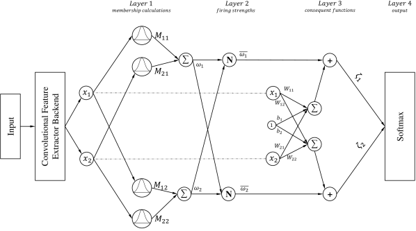
Figure 1: Simplified Block Diagram of our Deep Convolutional Neuro-Fuzzy Classifier

$$\begin{array}[hbt]{c}\displaystyle M_{ji}=\exp(-\beta_{ji}\cdot(x_{j}-\mu_{ji})^{2})\ \ \ \ \ \ \ \ \ _{(ANFIS)}\\ \displaystyle M_{ji}=-0.5\cdot\beta_{ji}\cdot(x_{j}-\mu_{ji})^{2}\ \ \ \ \ \ \ \ \ _{(DCNFIS)}\end{array}$$ (2)

Layer 2 computes the firing strength of each fuzzy rule. This is usually the product of all antecedent membership functions; however, as we are using logarithms, we sum the log memberships

$$\begin{array}[hbt]{c}\displaystyle\omega_{i}=\prod_{j}M_{ji}\ \ \ \ {}_{(ANFIS)}\\ \displaystyle\omega_{i}=\sum_{j}M_{ji}\ \ \ \ {}_{(DCNFIS)}\end{array}$$ (3)

In layer 3, the activation is normally computed as a linear combination of the input variables, multiplied by the normalized firing strength of the respective rule. This is changed to the sum of the log firing strength and the linear combination of the input variables.

$$\begin{array}[]{c}\displaystyle\zeta_{i}=\bar{\omega}_{i}\cdot(\sum_{j}W_{ji}\cdot x_{j}+b_{i})\ \ \ \ \ _{(ANFIS)}\\ \displaystyle\zeta_{i}=\bar{\omega}_{i}+(\sum_{j}W_{ji}\cdot x_{j}+b_{i})\ \ \ _{(DCNFIS)}\end{array}$$ (4)

Note that we do not take the logarithm of the linear combination of inputs. This modification allows us to create fuzzy regions (clusters) along with an end-to-end trainable deep convolutional backend without causing an error gradient explosion.

Finally, layer 4 computes the class probabilities using the softmax activation function

$$\begin{array}[]{c}\displaystyle P\left(c_{i}\middle|\ x\right)=y_{i}=\frac{\exp{\left(\zeta_{i}\right)}}{\sum_{o}{\exp{\left(\zeta_{o}\right)}}}\end{array}$$ (5)

This architecture mimics the operation of a Fuzzy Inferential System (FIS), which is a rule-based expert system (and thus highly interpretable). Specifically, the layer transfer functions mimic the stages of processing by which an FIS infers an output from its inputs. The hybrid learning rule for ANFIS (a Kalman filter in Layer 4, gradient descent for Layer 1) allows the fuzzy rule-base to be induced from a dataset. There is a 1:1 correspondence between ANFIS and the FIS it mimics, and so we can directly translate a trained ANFIS into fuzzy rules. However, this only applies to the direct inputs of ANFIS - which are the outputs of the final CNN layer. We defer further discussion of this point to our discussion of future work in Section 6.

Algorithm 1 Modified ANFIS

$N_{C}\leftarrow$ Number of output classes (number of rules)

$N_{V}\leftarrow$ Number of extracted features by CNN (number of input variables to ANFIS)

$M_{ji}\leftarrow$ Membership value of variable $j$ to membership functions of rule $i$

// Layer 1

for $i$ from 1 to $N_{C}$ do

     $\omega_{i}=0$

     for for $j$ from 1 to $N_{V}$ do

         $M_{ji}=-0.5\cdot\beta_{ji}\cdot(x_{j}-\mu_{ji})^{2}$

         $\omega_{i}=\omega_{i}+M_{ji}$

     end for

end for

// Layer 2

$\bar{\omega}=0$

for $i$ from 1 to $N_{C}$ do

     $\bar{\omega}=\bar{\omega}+\omega_{i}$

end for

for $i$ from 1 to $N_{C}$ do

     $\bar{\omega_{i}}=\frac{\omega_{i}}{\bar{\omega}}$

end for

// Layer 3

for $i$ from 1 to $N_{C}$ do

     $c_{i}=0$

     for for $j$ from 1 to $N_{V}$ do

         $c_{i}=c_{i}+W_{ji}\cdot x_{j}$

     end for

end for

for $i$ from 1 to $N_{C}$ do

     $\zeta_{i}=\bar{\omega_{i}}+c_{i}$

end for

// Layer 4

Send $\zeta_{i}$ to softmax activation function accourding to e.q. 5

Note that ANFIS does not provide a shortcut to the softmax layer. Layer 3 of ANFIS implements a linear combination of the network inputs for each individual rule. In the basic ANFIS, the rule is weighted by its firing strength (computed in Layer 2), and then passed to a summation. In our implementation, we have taken the logarithm of the network signals, and so we add the log of the firing strength to the weighted sum in Layer 3, and then pass the sum to the softmax function in Layer 4. As the logarithm function is monotonic increasing, the ranks of the softmax outputs should be the same as for the original ANFIS, even if the logit values have changed. Algorithm 1 shows the feed forward calculations for DCNFIS in detail. Based on this algorithm order of growth for the classifier of DCNFIS is $O(N_{C}\cdot N_{V})$. Our FLOPS comparison using model-profiler shows no difference between DCNFIS ResNet29_V2 and it’s regular version. This can be generally claimed that DCNFIS will have more parameters (for calculating membership funcions) in comparison with the regular CNN if the CNN’s classifier is not a multi-layer perceptron with hidden layers. In these situations, the number of extra parameters of DCNFIS can be calculated by $2*N_{C}*N_{V}$ which relates to the $\beta$ and $\mu$ parameters of membership functions for the rule-generation part of classifier.

IV-C Learning Algorithm

Our fuzzy classifier will use the Adam [32] algorithm for learning the adaptive parameters of the network. Adam optimization is a stochastic gradient descent method that is based on adaptive estimation of first-order and second-order moments. Thus, in order to update the parameters ($\theta$) ADAM first calcualtes gradients at time-step $t$, and then based on values of $\beta_{1}$ and $\beta_{2}$ bias-corrected first $(\hat{m_{t}})$ and second $(\hat{v_{t}})$ moment parameters will be updated. Finally the parameters will be updated based on: $\theta_{t}=\theta_{t-1}-\alpha\cdot\frac{\hat{m_{t}}}{\sqrt{\hat{v_{t}}+\epsilon}}$ where $\alpha$ is the step-size and $\epsilon=10e-8$. The gradients passed to the convolutional layers are calculated as follows:

$$\begin{array}[]{c}\displaystyle\frac{\partial\zeta_{i}}{\partial x_{j}}=\frac{\partial}{\partial x_{j}}{\omega_{i}}+\sum_{j}\ W_{ji}\\ \displaystyle=\frac{\partial}{\partial x_{j}}{\left(M_{ji}\right)}+\sum_{j}\ W_{ji}\\ \displaystyle=-\beta_{ji}\cdot\left(x_{j}-\mu_{ji}\right)+\sum_{j}\ W_{ji}\end{array}$$ (6)

Where the gradients of the membership function parameters can be calculated as follows:

$$\begin{array}[]{cccc}\vspace{1mm}\displaystyle\frac{\partial\zeta_{i}}{\partial\omega_{i}}=1\\ \vspace{1mm}\displaystyle\frac{\partial\zeta_{i}}{\partial M_{ji}}=1\\ \vspace{1mm}\displaystyle\frac{\partial\zeta_{i}}{\partial\mu_{ji}}=\beta_{ji}\left(x_{j}-\mu_{ji}\right)\\ \vspace{1mm}\displaystyle\frac{\partial\zeta_{i}}{\partial\beta_{ji}}=-0.5\cdot\left(x_{j}-\mu_{ji}\right)^{2}\end{array}$$ (7)

IV-D Guided Backpropagation

Guided backpropagation [120], is a new variant of the “deconvolution approach” for visualizing features learned by CNNs. Guided backpropagation allows the flow of only the positive gradients by changing the negative gradient values to zero. Fig. 2 shows a simple visualization on how guided backpropagation works. For details about comparison of saliency analysis methods see [121, 14].

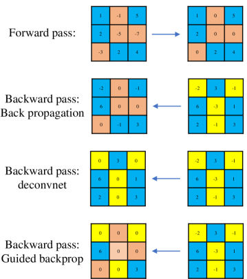
Figure 2: a simple visualization on guided backpropagation

IV-E Experimental Setup

The existing literature on all four datasets reports results based on a single-split design; for comparability we will follow this design, employing the same test set of 10,000 images as our out-of-sample evaluation. We test LeNet [37] with our modifications, then ResNet and Wide ResNet. Our tests employ the second version of ResNet20 [42] for MNIST, ResNet29 for Fashion MNIST, and ResNet164 for CIFAR-10 and CIFAR-100. We have tested WRN-28-10 for CIFAR-10, and WRN-28-12 for CIFAR-100 [43].

The LeNet-based architectures, are trained for 200 epochs in batches of 128. The parameters for the Adam optimizer have been set as $\eta=0.001$, $\beta_{1}=0.9$, $\beta_{2}=0.999$. For the ResNet and WRN-based experiments the models were trained for 200 epochs in batches of 128. The learning rate has been set to 0.001 initially, and then it will be reduced to 1e-6 after epoch 180. Data augmentation techniques are applied on all datasets except MNIST. All the experiments are replicated ten times.

V Evaluation

As shown in TABLE I, the performance difference between the original CNNs and their DCNFIS versions is very minor; about half the time, the base architecture was slightly better, and half the time the DCNFIS was better. This is a significant change from [29] and [30], in which the enhanced interpretability of the deep fuzzy system came at the price of clearly losing some overall accuracy.

We next conduct a statistical analysis of these results. As there are only ten replicates of each experiment, but the variances for the original CNN and the DCNFIS versions can be substantially different, we employ the $t$-test for unequal variances. At a significance level of $\alpha$ = 0.05, there are only two instances where the differences were significant: CIFAR-10 with ResNet, and CIFAR-100 with WRN. We thus claim that using the DCNFIS method does not appear to reduce the accuracy of a CNN.

TABLE I: DCNFIS and Regular-CNNs Accuracy Comparison

Dataset	LeNet
	Regular		DCNFIS
	AVG	STD	AVG	STD
MNIST	99.21	0.0404	99.23	0.462
Fashion-MNIST	90.36	0.2364	90.10	0.1445
CIFAR-10	73.11	0.4550	73.39	0.9267
CIFAR-100	43.25	0.6594	43.30	0.5472
	ResNet
	Regular		DCNFIS
	AVG	STD	AVG	STD
MNIST	99.57	0.381	99.59	0.0288
Fashion-MNIST	94.64	0.0816	94.401	0.2308
CIFAR-10	93.13a	0.0844	93.02	0.0526
CIFAR-100	74.52	0.0978	74.52	0.1589
	WRN
	Regular		DCNFIS
	AVG	STD	AVG	STD
CIFAR-10	96.620	0.23870	96.680	0.1789
CIFAR-100	78.50a	0.1077	77.53	0.3523

$a$-Significant at $\alpha$ = 0.05

We compare performance of DCNFIS with existing fuzzy methods in Table II. This table is sorted based on accuracy of methods on CIFAR-10 dataset.

TABLE II: DCNFIS and Other Fuzzy Methods Accuracy Comparison

id	MNIST	Fashion-MNIST	CIFAR-10 $\downarrow$	CIFAR-100
DCNFIS	99.59	94.4	96.68	77.53
Deep_GK [30, 29]	99.55	92.03	91.87
[76]	97.3	-	88.2	-
[77]	99.58	-	88.18	63.31
[55]	-	93.32	82.68	-
[53]	98.56	88.57	78.35	-
[54]	-	-	77.49	-
[81]	97.03	61.8	68.76	33.59
Deep_FCM [31, 29]	96.92	79.69	59.29	-
[83]	96	-	43.54	-
[84]	98	-	38	-
[52]	93.44	-	31.42	-
GK [29]	81.61	73.1	28.59	-
[56]	95.96	-	27.83	-
FCM [31, 29]	84.48	74.24	22.66	-
[86]	-	-	22.03	-

VI Interpretability

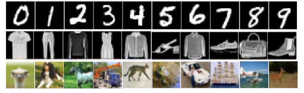
Figure 3: Class representatives derived from fuzzy rules. Top row: MNIST. Middle row: Fashion-MNIST. Bottom row: CIFAR-10

As discussed in section 4, DCNFIS uses the rule-based ANFIS architecture as its classifier component. Each rule in ANFIS is of the form of Eq. 8, and forms a conjunction of antecedent clauses, each represented by one fuzzy subset of the corresponding input dimension. The rule itself thus defines a fuzzy region of the ANFIS input space. The collection of feature vectors within this fuzzy region can be considered a fuzzy cluster. Following [29] we select the medoid element of a cluster as the representative for that cluster. The following equation shows the if-then rules of our modified ANFIS.

$$\begin{array}[]{c}\displaystyle If\ f_{1}\left(p_{1}\right)\ \ is\ M_{K,1}\ and\ f_{2}\left(p_{2}\right)\ is\ M_{K,2}\ and\dots\\ \displaystyle\ f_{D}\left(P_{D}\right)\ is\ \ M_{K,N}\ \ then\\ \displaystyle\log{P\left(c_{K}\middle|image\right)}=\ \sum_{i}{W_{K,i}f_{i}\left(P_{i}\right)+b_{k}}\end{array}$$ (8)

In Fig. 3, we present the medoid elements of the ten rules generated for each of our datasets (excluding CIFAR-100). Our approach to XAI is to treat the medoid as a synopsis of the entire cluster, with the saliency map computed using [122] for it constituting our explanans for the cluster. The general process is to train DCNFIS, and extract the fuzzy regions for each rule of the classifier. The region is treated as a fuzzy cluster, and the medoid element is identified. Next, we perform a saliency analysis on the medoids, using the Guided Backpropagation algorithm [120]. As the medoid element is arguably the most representative of the whole class, we build our explanations on the saliency maps of the ten medoids. More details on the method, and an empirical evaluation of different saliency analyses, can be found in [29, 30]. The power of DCNFIS in comparison with previous methods described in[31, 29, 30] is that, by contrast, all the medoids are extracted from the rules of DCNFIS; there is no need for any further post training clustering and classification process.

We next demonstrate our medoid-based explanans on Fashion-MNIST. Our discussion in this section is inspired by our previous analysis of the MNIST Digits dataset in [29]; we focus on examining selected misclassifications in the training dataset, comparing the saliency map of the erroneous examples against the saliency maps for the medoid images in the actual and predicted classes. As a contrast, we also examine selected correct classifications from the training dataset. Following this, we use UMAP visualizations to examine the misclassifications more formally. Finally, we discuss how our explanans were useful in detecting a learning bias being introduced in our model due to a commonly-used preprocessing step.

Fig. 4 presents the class medoids derived from the fuzzy rules for the Fashion-MNIST dataset. The top row is the medoid element of each cluster/class (labeled from left to right T-shirt/Top, Trouser, Pullover, Dress, Coat, Sandal, Shirt, Sneaker, Bag, and Ankle Boot), and the bottom row is the corresponding saliency map.

VI-A Fashion-MNIST

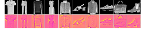
Figure 4: Class representatives derived from fuzzy rules for Fashion-MNIST dataset. First row: Medoids. Second row: Saliency of Medoids

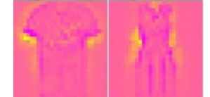
Figure 5: Difference between T-Shirt and Dress

One of the challenges with Fashion-MNIST is the similarity of some of the classes to each other. The images and labels were taken from the Zalando online store; the labels specifically are the “silhouette code” for that item, which is manually assigned by Zalando’s fashion staff (and then cross-checked by a separate team). Thus, while the labels are reliable, the distinctions between some classes are plainly finer than others. Coats and Pullovers, for instance, are only distinguished by the presence of a vertical zipper or line of buttons in the former, while the difference between a Coat and a Sandal is far more dramatic. The distinction between T-Shirt/Top and Dress is another example. As shown in Fig. 4, the shapes formed by yellow pixels (strong negative impact on class assignment) are the main difference between these two classes. In Fig. 5 we have focused on this difference. For class Dress the neural network doesn’t care about having a short or long sleeve. It focuses on detection of a long almost vertical yellow line which starts from the axilla and ends at the high hip. For T-Shirts the vertical yellow pixels starting from the axilla peter out around the mid-torso. Meanwhile, a strong region of yellow pixels can be observed directly under the cutoff of each sleeve; long sleeves would thus strongly contraindicate the T-Shirt/Top class.

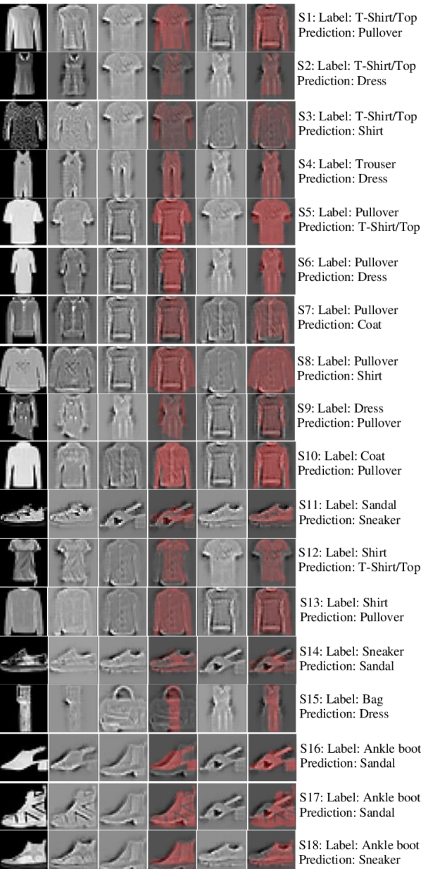
Figure 6: Images Misclassified by DCNFIS

Our analysis of DCNFIS misclassifications begins with an examination of misclassified images, presented in Fig. 6. We selected 18 misclassified examples from the Fashion-MNIST training data. Note that this particular model has a training accuracy of 98.096 percent, so only 1,146 samples out of 60,000 are misclassified. In this figure the original samples and their saliencies are shown in the first and second columns. In the third column we show the saliency of the medoid of the actual (label) class while in the fifth column we show the saliency of the predicted class. In columns four and six we overlay the saliencies of the sample on the saliencies from the label and prediction class medoids. For example, S1 is a T-Shirt/Top sample with long sleeves which is classified as a Pullover, and S2 is a T-Shirt/Top sample which has been found to be more similar to a Dress. This latter is an exemplar of a particularly challenging aspect of the T-Shirt/Top class, which we discuss in Section VI.B. What we see throughout these images is that the saliencies of each sample are noticeably more similar to the medoid of the predicted class (and the high-importance pixels especially so) than to the medoid of the labelled class. As in [29], this evidence tends to support our contention that the medoid saliences effectively capture the classification decisions of DCNFIS.

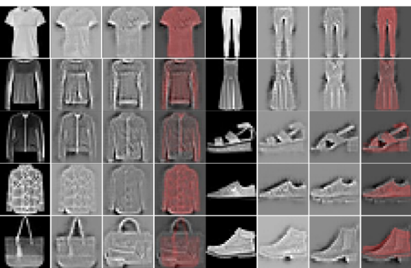
Figure 7: Samples Correctly Classified by DCNFIS

Fig. 7 shows 10 samples (one for each class) that are correctly classified by DCNFIS. Each row shows samples of two different classes. For each class, the first image shows the original sample, and the second image shows the saliency of the sample. The third image is the saliency of the class medoid, and the two saliences are overlaid in the fourth image, similar to columns of Fig. 6. As shown in the figure, the sample and medoid saliencies are very similar. For example, an ankle boot (bottom right) sample has been classified by detection of the heel and upper surface of the boot.

Hendricks et al. [123] proposed two criteria for explanations in image classification problems: they must be class discriminative, and image relevant. In that work, Hendricks et al. build natural language texts as explanations, so image relevance is a significant challenge. However, the more general point they raise is that explanations must refer to the specific content of the image in question. Understood in this fashion, we argue that our discussion above shows that the medoid-based approach is indeed image relevant. Indeed, each row of Fig. 6 compares the saliencies of a specific image against the actual and predicted class medoid saliencies, and highlights their similarities and differences. Class discriminativeness, meanwhile, is demonstrated in Fig. 4.

VI-B Global explanation or local?

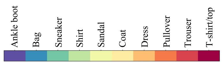
(a)

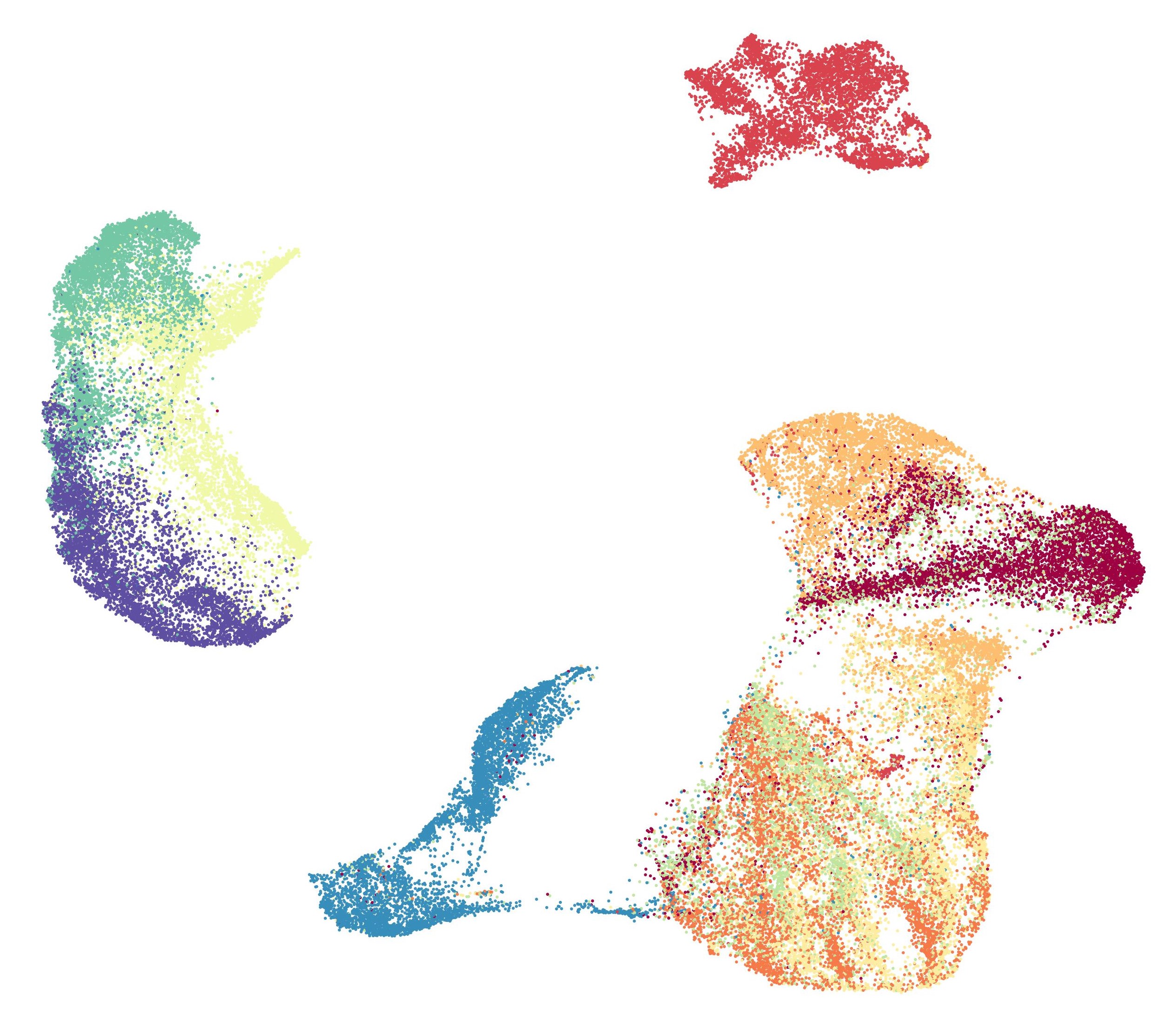
(b)

(c)

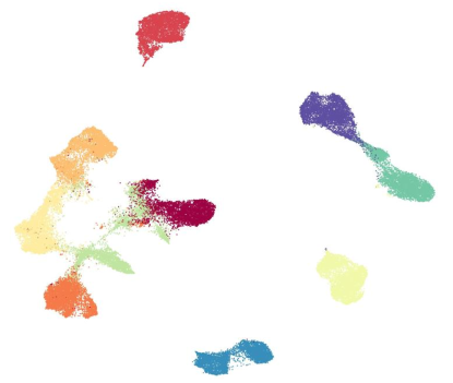
(d)

Figure 8: Left) 2-D UMAP visualization of Fashion-MNIST Dataset. Right) 2-D UMAP visualization of the DCNFIS Classifier Component Inputs (outputs from ResNet 29)

One of the principal advantages of CNNs is that the convolutional component acts as an automated feature selection algorithm. As DCNFIS does not change the convolution components of the base architecture, we expect that it will remain effective in this role. However, as DCNFIS is an end-to-end trainable algorithm, this expectation needs to be checked; the error signals being propagated through the fuzzy classifier component will, after all, be different than those propagated from layers of dense and SoftMax neurons. In this section, we thus evaluate this expectation on the Fashion-MNIST dataset, by visualizing the original dataset, and the outputs of the trained convolutional component, using the Uniform Manifold Approximation and Projection (UMAP) algorithm. We then further investigate selected misclassifications in these visualizations.

Left figure in Fig. 8 shows a 2-dimensional visualization of the Fashion-MNIST training dataset, created using UMAP [124] with its default parameters. The Shirt, Coat, Dress, Pullover, and T-shirt/Top classes are badly comingled at the lower right, while the Ankle Boot, Sneaker and Sandal classes also overlap heavily at the upper left. Only the Trouser and Bag classes are well-separated. Right figure in Fig. 8 is a UMAP visualization (using the same parameters) of the training data output of the convolutional component of a trained DCNFIS network (i.e. the input to the fuzzy classifier). Plainly, there is a substantial improvement in the separation of the different classes (interpreting the compactness of the classes is more difficult, as UMAP is a nonlinear projection that balances preservation of local and global structure).

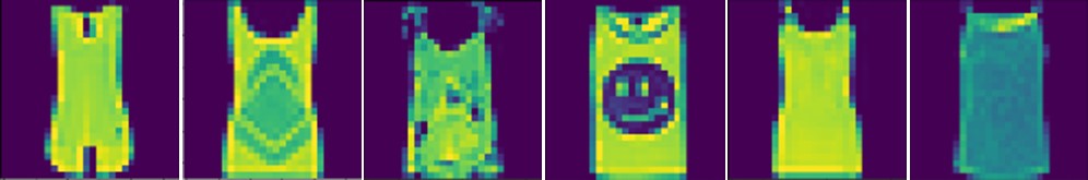
Figure 9: Visualization of 6 samples of Top images out of 32

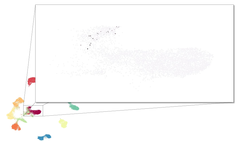
Figure 10: Visualization of 32 selected Top samples out in the T-shirt/Top class region

However, an important characteristic of our medoid-based explanans can be observed in the T-shirt/Top class. We manually selected the sequentially first 32 images in this class that do not resemble T-shirts (i.e. that are sleeveless; Fig. 9 presents 6 such examples). All but one of the 32 are correctly classified, but they do not closely resemble the T-shirt/Top medoid from Fig. 4 (leftmost image). When we highlight these 32 examples in Fig. 10, we find that they all occur in the “upper” lobe of the class distribution, which appears to hold a concentration of examples at some distance from the class medoid. In this context, the misclassification of a Top as a Dress in Fig. 5 is revealing; sleeveless tops seem to lie in a different grouping from the class medoid. It is possible that splitting the T-shirt/Top class into separate clusters might yield a new medoid that better represents the Tops. Put another way, the T-shirt/Top class may well consist of multiple disjuncts. In general, our medoid-based approach is likely to struggle with such classes, especially when the class is arguably a conflation of multiple real-world concepts. In these scenarios we should consider the explanation only as a local explanation as the medoid is not a good representative of the entire cluster.

VI-C Bias in Fashion-MNIST

One of the use cases for XAI is in debugging trained AI systems. Our experiments with DCNFIS unexpectedly offered a demonstration of this use case on the Fashion-MNIST dataset. One of the common preprocessing steps for image data is to subtract the per-pixel mean of the dataset from all images [41] (a zero-mean dataset is somewhat easier to train, as has been well-known for decades [6]). However, in our experiments, we were finding that DCNFIS was noticeably less accurate than the base CNNs. When we look at our saliency maps, a reason for this appears, as in Fig. 11.

What we see in these medoid saliencies (for the Sandal, Sneaker, and Ankle Boot classes) is what appears to be the faint image of some sort of top, indicated by pixels with negative saliency. However, no such structure appears in the actual images. The reason for this lies in an apparent bias of the Fashion-MNIST dataset; as has been noted, four of the ten classes are some sort of upper-body garment, and the Dress class is also similar. As a result, when we plot the per-pixel means as an image, we obtain the following (Fig. 12).

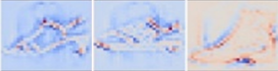
Figure 11: Medoids of DCNFIS for classes of Sandal, Sneaker, Ankle-Boot from training data with mean subtraction

Figure 12: Mean of training data visualized as an image

TABLE III: Confusion Matrix of DCNFIS with mean subtraction

	T-shirt top	Pullover	Coat	Shirt	Dress	Trouser	Sandal	Sneaker	Ankle boot	Bag
T-shirt top	5671	41	2	227	56	0	1	0	0	2
Pullover	58	5601	176	130	32	1	0	0	0	2
Coat	1	29	5833	84	49	2	0	0	0	2
Shirt	326	94	109	5377	90	1	0	0	0	3
Dress	21	6	68	27	5875	2	0	0	0	1
Trouser	1	1	1	3	15	5978	0	0	0	1
Sandal	0	0	0	0	0	0	5981	16	0	2
Sneaker	0	0	0	0	0	0	15	5925	60	0
Ankle boot	0	0	0	0	0	0	19	105	5874	2
Bag	0	0	1	1	2	0	0	0	0	5996

TABLE IV: Confusion Matrix of DCNFIS without mean subtraction

	T-shirt top	Pullover	Coat	Shirt	Dress	Trouser	Sandal	Sneaker	Ankle boot	Bag
T-shirt top	5759	19	3	192	21	0	1	0	0	5
Pullover	35	5809	75	72	9	0	0	0	0	0
Coat	0	33	5888	55	24	0	0	0	0	0
Shirt	156	75	77	5645	44	1	0	0	0	2
Dress	7	5	28	33	5926	0	0	0	0	1
Trouser	0	0	0	1	4	5995	0	0	0	0
Sandal	0	0	0	0	0	0	5984	13	3	0
Sneaker	0	0	0	0	0	0	11	5942	46	1
Ankle boot	0	0	0	0	0	0	3	84	5913	0
Bag	0	0	1	1	1	0	0	0	0	5997

We see what seems like the silhouette of a long-sleeved top garment of some sort, with pant-like structures in the lower 2/3rds of the image. The outer edges of the pants, however, seem to line up with the presumptive axilla on the top garment, thus reinforcing its shape. This observation caused us to run a further set of experiments, without mean removal. In Tables III and TABLE IV, we present the confusion matrices produced by DCNFIS on the training dataset with and without mean subtraction, respectively. Plainly, eliminating mean removal improved our accuracy; the total impact was four tenths of a percentage point on the test data, which is greater than the standard deviation of our ten replications (see Table I). In other words, the error introduced by mean subtraction was sufficient to significantly alter the outcomes of our experiments. Thus, our observations in this section serendipitously demonstrate that our medoid-based explanans on DCNFIS can be effective in debugging an AI

VII Conclusion

In this paper we have proposed a novel deep fuzzy network, which replaces the dense layers at the terminal end of a deep CNN with an ANFIS network. The architecture is end-to-end trainable, remains as accurate as the base CNNs is built from, and our medoid-based saliency-map explanations derived from the fuzzy rules seem more effective than extracting saliency maps for each data sample.

In future work, we will explore fuzzy classifiers with multiple clusters mapping to a single class. We will also explore a radically different explanation mechanism: since we already have a fuzzy inference system as the final classifier for this network, it should be possible to back-propagate the fuzzy sets to the input feature space, forming a new set of fuzzy rules directly mapping inputs to the final network outputs as a linguistic explanation

References

- [1] C. Szegedy, W. Liu, Y. Jia, P. Sermanet, S. Reed, D. Anguelov, D. Erhan, V. Vanhoucke, and A. Rabinovich, “Going deeper with convolutions,” in Proceedings of the IEEE conference on computer vision and pattern recognition, 2015, pp. 1–9.
- [2] I. Sutskever, O. Vinyals, and Q. V. Le, “Sequence to sequence learning with neural networks,” in Advances in neural information processing systems, 2014, pp. 3104–3112.
- [3] T. N. Sainath, B. Kingsbury, G. Saon, H. Soltau, A. rahman Mohamed, G. Dahl, and B. Ramabhadran, “Deep Convolutional Neural Networks for Large-scale Speech Tasks,” Neural Networks, vol. 64, 2015.
- [4] A. Soleymani, A. A. S. Asl, M. Yeganejou, S. Dick, M. Tavakoli, and X. Li, “Surgical skill evaluation from robot-assisted surgery recordings,” in 2021 International Symposium on Medical Robotics (ISMR). IEEE, 2021, pp. 1–6.
- [5] M. Yeganejou, M. Keshmiri, and S. Dick, “Accurate and explainable retinal disease recognition via DCNFIS,” in Fuzzy Information Processing: 42th Conference of the North American Fuzzy Information Processing Society, NAFIPS 2023, Cincinnati, OH, USA, Proceedings 42. Springer, 2023.
- [6] S. Haykin, Neural Networks and Learning Machines, 3rd Ed. Upper Saddle River: Pearson Education, Inc., 2009.
- [7] M. T. Ribeiro, S. Singh, and C. Guestrin, “Why should i trust you?: Explaining the predictions of any classifier,” in Proceedings of the 22nd ACM SIGKDD international conference on knowledge discovery and data mining. ACM, 2016, pp. 1135–1144.
- [8] R. Caruana, Y. Lou, J. Gehrke, P. Koch, M. Sturm, and N. Elhadad, “Intelligible Models for HealthCare: Predicting Pneumonia Risk and Hospital 30-day Readmission,” in 21st ACM SIGKDD International Conference on Knowledge Discovery and Data Mining (KDD ’15), Proceedings, 2015.
- [9] D. Baehrens, T. Schroeter, S. Harmeling, M. Kawanabe, K. Hansen, and K.-R. MÞller, “How to explain individual classification decisions,” Machine Learning Research 11(Jun)., 2010.
- [10] L. R. Ye and P. E. Johnson, “The impact of explanation facilities on user acceptance of expert systems advice,” Mis Quarterly, pp. 157–172, 1995.
- [11] U. Fayyad, G. Piatetsky-Shapiro, and P. Smyth, “Knowledge Discovery and Data Mining: Towards a Unifying Framework.” Int Conf on Knowledge Discovery and Data Mining, 1996.
- [12] S. Hajian, F. Bonchi, and C. Castillo, “Algorithmic bias: From discrimination discovery to fairness-aware data mining,” in Proceedings of the ACM SIGKDD International Conference on Knowledge Discovery and Data Mining, 2016.
- [13] B. Goodman and S. Flaxman, “European union regulations on algorithmic decision making and a ”right to explanation”,” AI Magazine, 2017.
- [14] M. Yeganejou and S. Dick, “Explainable Artificial Intelligence and Computational Intelligence: Past and Present,” HANDBOOK ON COMPUTER LEARNING AND INTELLIGENCE: Volume 2: Deep Learning, Intelligent Control and Evolutionary Computation, pp. 3–55, 2022.
- [15] R. Goebel, A. Chander, K. Holzinger, F. Lecue, Z. Akata, S. Stumpf, P. Kieseberg, and A. Holzinger, “Explainable AI: the new 42?” in International cross-domain conference for machine learning and knowledge extraction. Springer, 2018, pp. 295–303.
- [16] H. Ishibuchi and Y. Nojima, “Discussions on Interpretability of Fuzzy Systems using Simple Examples.” in IFSA/EUSFLAT Conf., 2009, pp. 1649–1654.
- [17] Z. C. Lipton, “The mythos of model interpretability,” Communications of the ACM, 2018.
- [18] A. B. Tickle, R. Andrews, M. Golea, and J. Diederich, “The truth will come to light: Directions and challenges in extracting the knowledge embedded within trained artificial neural networks,” IEEE Transactions on Neural Networks, 1998.
- [19] J. R. Zilke, E. Loza Mencía, and F. Janssen, “DeepRED – Rule Extraction from Deep Neural Networks,” Discovery Science 19th International Conference, 2016.
- [20] M. D. Zeiler, D. Krishnan, G. W. Taylor, and R. Fergus, “Deconvolutional networks,” in Proceedings of the IEEE Computer Society Conference on Computer Vision and Pattern Recognition, 2010.
- [21] S. Bach, A. Binder, G. Montavon, F. Klauschen, K. R. Müller, and W. Samek, “On pixel-wise explanations for non-linear classifier decisions by layer-wise relevance propagation,” PLoS ONE, 2015.
- [22] S. K. Pal and S. Mitra, “Multilayer Perceptron, Fuzzy Sets, and Classification,” IEEE Transactions on Neural Networks, 1992.
- [23] J. S. R. Jang, “ANFIS: Adaptive-Network-Based Fuzzy Inference System,” IEEE Transactions on Systems, Man and Cybernetics, 1993.
- [24] M. J. Gacto, R. Alcalá, and F. Herrera, “Interpretability of linguistic fuzzy rule-based systems: An overview of interpretability measures,” Information Sciences, 2011.
- [25] M. T. Ribeiro, S. Singh, and C. Guestrin, “Model-agnostic interpretability of machine learning,” arXiv preprint arXiv:1606.05386, 2016.
- [26] H. Ishibuchi and Y. Nojima, “Analysis of interpretability-accuracy tradeoff of fuzzy systems by multiobjective fuzzy genetics-based machine learning,” International Journal of Approximate Reasoning, vol. 44, no. 1, pp. 4–31, 2007.
- [27] F. Chollet, Deep learning with Python. Simon and Schuster, 2021.
- [28] M. Yeganejou, R. Kluzinski, S. Dick, and J. Miller, “An End-to-End Trainable Deep Convolutional Neuro-Fuzzy Classifier,” in 2022 IEEE International Conference on Fuzzy Systems (FUZZ-IEEE). IEEE, 2022, pp. 1–7.
- [29] M. Yeganejou, S. Dick, and J. Miller, “Interpretable Deep Convolutional Fuzzy Classifier,” IEEE Transactions on Fuzzy Systems, vol. 28, no. 7, pp. 1407–1419, 2020.
- [30] M. Yeganejou and S. Dick, “Improved deep fuzzy clustering for accurate and interpretable classifiers,” in 2019 IEEE international conference on fuzzy systems (FUZZ-IEEE). IEEE, 2019, pp. 1–7.
- [31] ——, “Classification via deep fuzzy c-means clustering,” in IEEE International Conference on Fuzzy Systems, 2018.
- [32] D. P. Kingma and J. Ba, “Adam: A method for stochastic optimization,” arXiv preprint arXiv:1412.6980, 2014.
- [33] R. E. Kalman, “A new approach to linear filtering and prediction problems,” Journal of Fluids Engineering, Transactions of the ASME, 1960.
- [34] S. Ovchinnikov, “Similarity relations, fuzzy partitions, and fuzzy orderings,” Fuzzy Sets and Systems, vol. 40, no. 1, pp. 107–126, 1991.
- [35] L. A. Zadeh, “The concept of a linguistic variable and its application to approximate reasoning-I,” Information Sciences, 1975.
- [36] L. Zadeh, “Fuzzy sets,” Information and Control, 1965.
- [37] Y. LeCun, L. Bottou, Y. Bengio, and P. Haffner, “Gradient-based learning applied to document recognition,” Proceedings of the IEEE, 1998.
- [38] A. Krizhevsky, I. Sutskever, and G. E. Hinton, “Imagenet classification with deep convolutional neural networks,” in Advances in neural information processing systems, 2012, pp. 1097–1105.
- [39] M. D. Zeiler and R. Fergus, “Visualizing and understanding convolutional networks,” in European conference on computer vision. Springer, 2014, pp. 818–833.
- [40] I. Arel, D. C. Rose, and T. P. Karnowski, “Deep Machine Learning - A New Frontier in Artificial Intelligence Research [Research Frontier],” IEEE Computational Intelligence Magazine, 2010.
- [41] K. He, X. Zhang, S. Ren, and J. Sun, “Deep residual learning for image recognition,” in Proceedings of the IEEE conference on computer vision and pattern recognition, 2016, pp. 770–778.
- [42] ——, “Identity mappings in deep residual networks,” in European conference on computer vision. Springer, 2016, pp. 630–645.
- [43] S. Zagoruyko and N. Komodakis, “Wide residual networks,” arXiv preprint arXiv:1605.07146, 2016.
- [44] J.-S. R. Jang, C.-T. Sun, and E. Mizutani, Neuro-Fuzzy and Soft Computing: A Computational Approach to Learning and Machine Intelligence, 1997.
- [45] A. Sarabakha and E. Kayacan, “Online Deep Fuzzy Learning for Control of Nonlinear Systems Using Expert Knowledge,” IEEE Transactions on Fuzzy Systems, 2020.
- [46] C. L. Chen, C. Y. Zhang, L. Chen, and M. Gan, “Fuzzy Restricted Boltzmann Machine for the Enhancement of Deep Learning,” IEEE Transactions on Fuzzy Systems, 2015.
- [47] R. R. Yager, “Pythagorean membership grades in multicriteria decision making,” IEEE Transactions on Fuzzy Systems, 2014.
- [48] Y.-J. Zheng, W.-G. Sheng, X.-M. Sun, and S.-Y. Chen, “Airline Passenger Profiling Based on Fuzzy Deep Machine Learning,” IEEE Transactions on Neural Networks and Learning Systems, 2016.
- [49] A. Shukla, T. Seth, and P. Muhuri, “Interval type-2 fuzzy sets for enhanced learning in deep belief networks,” in IEEE International Conference on Fuzzy Systems, 2017.
- [50] S. Feng, C. L. Philip Chen, and C. Y. Zhang, “A Fuzzy Deep Model Based on Fuzzy Restricted Boltzmann Machines for High-Dimensional Data Classification,” IEEE Transactions on Fuzzy Systems, 2020.
- [51] Y. J. Zheng, S. Y. Chen, Y. Xue, and J. Y. Xue, “A Pythagorean-Type Fuzzy Deep Denoising Autoencoder for Industrial Accident Early Warning,” IEEE Transactions on Fuzzy Systems, 2017.
- [52] T. Sharma, V. Singh, S. Sudhakaran, and N. K. Verma, “Fuzzy based pooling in convolutional neural network for image classification,” in 2019 IEEE International Conference on Fuzzy Systems (FUZZ-IEEE). IEEE, 2019, pp. 1–6.
- [53] D. E. Diamantis and D. K. Iakovidis, “Fuzzy pooling,” IEEE Transactions on Fuzzy Systems, vol. 29, no. 11, pp. 3481–3488, 2020.
- [54] A. Beke and T. Kumbasar, “Interval type-2 fuzzy systems as deep neural network activation functions,” in 11th Conference of the European Society for Fuzzy Logic and Technology (EUSFLAT 2019). Atlantis Press, 2019, pp. 267–273.
- [55] Y. Bodyanskiy and S. Kostiuk, “Deep neural network based on f-neurons and its learning,” 2022.
- [56] T. Sharma, N. K. Verma, and S. Masood, “Mixed fuzzy pooling in convolutional neural networks for image classification,” Multimedia Tools and Applications, vol. 82, no. 6, pp. 8405–8421, 2023.
- [57] S. Zhang, Z. Sun, M. Wang, J. Long, Y. Bai, and C. Li, “Deep Fuzzy Echo State Networks for Machinery Fault Diagnosis,” IEEE Transactions on Fuzzy Systems, 2020.
- [58] L. X. Wang, “Fast Training Algorithms for Deep Convolutional Fuzzy Systems with Application to Stock Index Prediction,” IEEE Transactions on Fuzzy Systems, 2020.
- [59] M. Pratama, W. Pedrycz, and G. I. Webb, “An Incremental Construction of Deep Neuro Fuzzy System for Continual Learning of Nonstationary Data Streams,” IEEE Transactions on Fuzzy Systems, 2020.
- [60] S. Liu, G. Lin, Q. L. Han, S. Wen, J. Zhang, and Y. Xiang, “DeepBalance: Deep-Learning and Fuzzy Oversampling for Vulnerability Detection,” IEEE Transactions on Fuzzy Systems, 2020.
- [61] Q. Feng, L. Chen, C. L. Philip Chen, and L. Guo, “Deep Fuzzy Clustering-A Representation Learning Approach,” IEEE Transactions on Fuzzy Systems, 2020.
- [62] P. Hurtik, V. Molek, and J. Hula, “Data Preprocessing Technique for Neural Networks Based on Image Represented by a Fuzzy Function,” IEEE Transactions on Fuzzy Systems, 2020.
- [63] L. Chen, W. Su, M. Wu, W. Pedrycz, and K. Hirota, “A Fuzzy Deep Neural Network with Sparse Autoencoder for Emotional Intention Understanding in Human-Robot Interaction,” IEEE Transactions on Fuzzy Systems, 2020.
- [64] C. Guan, S. Wang, and A. W.-C. Liew, “Lip image segmentation based on a fuzzy convolutional neural network,” IEEE Transactions on Fuzzy Systems, 2019.
- [65] Y. Wang, Q. Hu, P. Zhu, L. Li, B. Lu, J. M. Garibaldi, and X. Li, “Deep Fuzzy Tree for Large-Scale Hierarchical Visual Classification,” IEEE Transactions on Fuzzy Systems, 2020.
- [66] A. I. Aviles, S. M. Alsaleh, E. Montseny, P. Sobrevilla, and A. Casals, “A deep-neuro-fuzzy approach for estimating the interaction forces in robotic surgery,” in 2016 IEEE International Conference on Fuzzy Systems, FUZZ-IEEE 2016, 2016.
- [67] S. Rajurkar and N. K. Verma, “Developing deep fuzzy network with Takagi Sugeno fuzzy inference system,” in IEEE International Conference on Fuzzy Systems, 2017.
- [68] T. Zhou, F. L. Chung, and S. Wang, “Deep TSK Fuzzy Classifier With Stacked Generalization and Triplely Concise Interpretability Guarantee for Large Data,” IEEE Transactions on Fuzzy Systems, 2017.
- [69] S. Gu, F.-L. Chung, and S. Wang, “A novel deep fuzzy classifier by stacking adversarial interpretable TSK fuzzy sub-classifiers with smooth gradient information,” IEEE Transactions on Fuzzy Systems, vol. 28, no. 7, pp. 1369–1382, 2019.
- [70] W. R. Tan, C. S. Chan, H. E. Aguirre, and K. Tanaka, “Fuzzy qualitative deep compression network,” Neurocomputing, 2017.
- [71] R. Jafari, S. Razvarz, and A. Gegov, “Neural Network Approach to Solving Fuzzy Nonlinear Equations Using Z-Numbers,” IEEE Transactions on Fuzzy Systems, 2020.
- [72] M. A. Islam, D. T. Anderson, A. J. Pinar, T. C. Havens, G. Scott, and J. M. Keller, “Enabling Explainable Fusion in Deep Learning with Fuzzy Integral Neural Networks,” IEEE Transactions on Fuzzy Systems, 2020.
- [73] V. John, S. Mita, Z. Liu, and B. Qi, “Pedestrian detection in thermal images using adaptive fuzzy C-means clustering and convolutional neural networks,” in 2015 14th IAPR International Conference on Machine Vision Applications (MVA), 2015.
- [74] Y. De la Rosa, Erick, Wen, “Data-Driven Fuzzy Modeling Using Deep Learning,” arXiv preprint arXiv:1702.07076 (2017).
- [75] Z. Zhang, M. Huang, S. Liu, B. Xiao, and T. S. Durrani, “Fuzzy Multilayer Clustering and Fuzzy Label Regularization for Unsupervised Person Reidentification,” IEEE Transactions on Fuzzy Systems, 2020.
- [76] S. Riaz, A. Arshad, and L. Jiao, “A semi-supervised cnn with fuzzy rough c-mean for image classification,” IEEE Access, vol. 7, pp. 49 641–49 652, 2019.
- [77] O. Yazdanbakhsh and S. Dick, “A deep neuro-fuzzy network for image classification,” arXiv preprint arXiv:2001.01686, 2019.
- [78] Y. Zhang, H. Ishibuchi, and S. Wang, “Deep Takagi-Sugeno-Kang Fuzzy Classifier With Shared Linguistic Fuzzy Rules,” IEEE Transactions on Fuzzy Systems, 2018.
- [79] T. Zhou, H. Ishibuchi, and S. Wang, “Stacked-structure-based hierarchical takagi-sugeno-kang fuzzy classification through feature augmentation,” IEEE Transactions on Emerging Topics in Computational Intelligence, vol. 1, no. 6, pp. 421–436, 2017.
- [80] X. Gu and P. P. Angelov, “Semi-supervised deep rule-based approach for image classification,” Applied Soft Computing, vol. 68, pp. 53–68, 2018.
- [81] D. Tan, Z. Huang, X. Peng, W. Zhong, and V. Mahalec, “Deep adaptive fuzzy clustering for evolutionary unsupervised representation learning,” IEEE Transactions on Neural Networks and Learning Systems, 2023.
- [82] F. Guo, J. Liu, M. Li, T. Huang, Y. Zhang, D. Li, and H. Zhou, “A concise tsk fuzzy ensemble classifier integrating dropout and bagging for high-dimensional problems,” IEEE Transactions on Fuzzy Systems, vol. 30, no. 8, pp. 3176–3190, 2021.
- [83] R. Shah, “Adaptive fuzzy network based transfer learning for image classification,” in 2020 IEEE International Students’ Conference on Electrical, Electronics and Computer Science (SCEECS). IEEE, 2020, pp. 1–4.
- [84] E. Di Nardo and A. Ciaramella, “Advanced fuzzy relational neural network.” in WILF, 2021.
- [85] Z. Xi and G. Panoutsos, “Interpretable machine learning: convolutional neural networks with rbf fuzzy logic classification rules,” in 2018 International conference on intelligent systems (IS). IEEE, 2018, pp. 448–454.
- [86] R. Zhang, X. Li, H. Zhang, and F. Nie, “Deep fuzzy k-means with adaptive loss and entropy regularization,” IEEE Transactions on Fuzzy Systems, vol. 28, no. 11, pp. 2814–2824, 2019.
- [87] K. Lazanyi, “Readiness for Artificial Intelligence,” in International Symposium on Intelligent Systems and Informatics (SISY), 2018, pp. 235–238.
- [88] M. Ashoori and J. D. Weisz, “In AI We Trust? Factors That Influence Trustworthiness of AI-infused Decision-Making Processes,” Tech. Rep., 2019.
- [89] D. H. McKnight and N. L. Chervany, “What trust means in e-commerce customer relationships: An interdisciplinary conceptual typology,” International journal of electronic commerce, vol. 6, no. 2, pp. 35–59, 2001.
- [90] P. Beatty, I. Reay, S. Dick, and J. Miller, “Consumer trust in e-commerce web sites: A meta-study,” ACM Computing Surveys, vol. 43, no. 3, pp. 14:1–14:46, 2011.
- [91] J. B. Rotter, “A new scale for the measurement of interpersonal trust.” Journal of personality, 1967.
- [92] T. R. Tyler, “Why People Obey the Law,” 1990.
- [93] D. M. Rousseau, S. B. Sitkin, R. S. Burt, and C. Camerer, “Not so different after all: A cross-discipline view of trust,” Academy of management review, vol. 23, no. 3, pp. 393–404, 1998.
- [94] R. C. Mayer, J. H. Davis, and F. D. Schoorman, “An Integrative Model Of Organizational Trust,” Academy of Management Review, vol. 20, no. 3, pp. 709–734, 1995.
- [95] J. Lyons, N. Ho, J. Friedman, G. Alarcon, and S. Guznov, “Trust of Learning Systems: Considerations for Code, Algorithms, and Affordances for Learning,” in Human and Machine Learning, J. Zhou and F. Chen, Eds. Cham: Springer International Publishing AG, 2018, pp. 265–278.
- [96] J. D. Lee and B. D. Seppelt, “Human Factors in Automation Design,” in Springer Handbook of Automation, S. Y. Nof, Ed. Berlin: Springer-Verlag, pp. 417–436.
- [97] J. B. Lyons and C. K. Stokes, “Human–Human Reliance in the Context of Automation,” Human Factors, vol. 54, no. 1, pp. 112–121, 2011.
- [98] L. Onnasch, C. D. Wickens, H. Li, and D. Manzey, “Human performance consequences of stages and levels of automation: An integrated meta-analysis,” Human Factors, vol. 56, no. 3, pp. 476–488, 2014.
- [99] J. D. Lee and K. A. See, “Trust in Automation: Designing for Appropriate Reliance,” Human Factors: The Journal of the Human Factors and Ergonomics Society2, vol. 46, no. 1, pp. 50–80, 4.
- [100] B. W. Israelsen and N. R. Ahmed, ““Dave…I can assure you …that it’s going to be all right …” A Definition, Case for, and Survey of Algorithmic Assurances in Human-Autonomy Trust Relationships,” pp. 1–37, 2019.
- [101] J. Drozdal, J. Weisz, D. Wang, G. Dass, B. Yao, C. Zhao, M. Muller, L. Ju, and H. Su, “Trust in AutoML: Exploring Information Needs for Establishing Trust in Automated Machine Learning Systems,” 2020. [Online]. Available: http://arxiv.org/abs/2001.06509%0Ahttp://dx.doi.org/10.1145/3377325.3377501
- [102] J. Overton, “Scientific Explanation and Computation.” in ExaCt, 2011, pp. 41–50.
- [103] T. Miller, “Explanation in Artificial Intelligence: Insights from the Social Sciences,” Artificial Intelligence, vol. 267, pp. 1–38, 2019.
- [104] E. Toreini, M. Aitken, K. Coopamootoo, K. Elliott, C. G. Zelaya, and A. van Moorsel, “The relationship between trust in AI and trustworthy machine learning technologies,” in FAT* 2020 - Proceedings of the 2020 Conference on Fairness, Accountability, and Transparency, 2020, pp. 272–283.
- [105] G. Dietz and D. N. D. Hartog, “Measuring trust inside organisations,” Personnel Review, vol. 35, no. 5, pp. 557–588, 2006.
- [106] F. D. Davis, “Perceived Usefulness, Perceived Ease of Use, and User Acceptance of Information Technology,” MIS Quarterly, vol. 13, no. 3, pp. 319–340, 1989.
- [107] S. Mohseni, N. Zarei, and E. D. Ragan, “A multidisciplinary survey and framework for design and evaluation of explainable AI systems,” 2018.
- [108] D. H. McKnight, V. Choudhury, and C. Kacmar, “Developing and validating trust measures for e-commerce: An integrative typology,” Information systems research, vol. 13, no. 3, pp. 334–359, 2002.
- [109] D. Gefen, I. Benbasat, and P. Pavlou, “A research agenda for trust in online environments,” Journal of Management Information Systems, vol. 24, no. 4, pp. 275–286, 2008.
- [110] P. B. Lowry, A. Vance, G. Moody, B. Beckman, and A. Read, “Explaining and predicting the impact of branding alliances and web site quality on initial consumer trust of e-commerce web sites,” Journal of Management Information Systems, vol. 24, no. 4, pp. 199–224, 2008.
- [111] R. Tomsett, D. Braines, D. Harborne, A. Preece, and S. Chakraborty, “Interpretable to whom? A role-based model for analyzing interpretable machine learning systems,” 2018.
- [112] W. A. Bainbridge, J. W. Hart, E. S. Kim, and B. Scassellati, “The Benefits of Interactions with Physically Present Robots over Video-Displayed Agents,” International Journal of Social Robotics, vol. 3, pp. 41–52, 2011.
- [113] G. J. Nalepa, M. van Otterlo, S. Bobek, and M. Atzmueller, “From context mediation to declarative values and explainability,” in Proceedings of the IJCAI/ECAI Workshop on Explainable Artificial Intelligence (XAI 2018). IJCAI, Stockholm, 2018.
- [114] V. Beaudouin, I. Bloch, D. Bounie, S. Clémençon, F. D’Alché-Buc, J. Eagan, W. Maxwell, P. Mozharovskyi, and J. Parekh, “Flexible and Context-Specific AI Explainability: A Multidisciplinary Approach,” SSRN Electronic Journal, 2020.
- [115] S. R. Islam, W. Eberle, and S. K. Ghafoor, “Towards quantification of explainability in explainable artificial intelligence methods,” in The thirty-third international flairs conference, 2020.
- [116] “Dataset, MNIST.” [Online]. Available: http://yann.lecun.com/exdb/mnist/
- [117] H. Xiao, K. Rasul, and R. Vollgraf, “Fashion-mnist: a novel image dataset for benchmarking machine learning algorithms,” arXiv preprint arXiv:1708.07747, 2017.
- [118] A. Krizhevsky, “Learning Multiple Layers of Features from Tiny Images,” … Science Department, University of Toronto, Tech. …, 2009.
- [119] C.-T. Sun and J.-S. Jang, “A neuro-fuzzy classifier and its applications,” in [Proceedings 1993] Second IEEE International Conference on Fuzzy Systems. IEEE, 1993, pp. 94–98.
- [120] J. T. Springenberg, A. Dosovitskiy, T. Brox, and M. Riedmiller, “Striving for simplicity: The all convolutional net,” arXiv preprint arXiv:1412.6806, 2014.
- [121] M. Yeganejou, “Interpretable Deep Covolutional Fuzzy Networks,” Ph.D. dissertation, University of Alberta, 2019. [Online]. Available: https://era.library.ualberta.ca/items/3e81868d-b0d8-4a25-a154-8d1f51ee293e
- [122] M. Alber, S. Lapuschkin, P. Seegerer, M. Hägele, K. Schütt, G. Montavon, W. Samek, K.-R. Müller, S. Dähne, and P.-J. Kindermans, “iNNvestigate neural networks!” arXiv preprint arXiv:1808.04260, 2018.
- [123] L. A. Hendricks, A. Rohrbach, B. Schiele, T. Darrell, and Z. Akata, “Generating visual explanations with natural language,” Applied AI Letters, vol. 2, no. 4, 2021.
- [124] L. McInnes and J. Healy, “Umap: Uniform manifold approximation and projection for dimension reduction,” arXiv preprint arXiv:1802.03426, 2018.