Majority Vote Computation With Complementary Sequences for Distributed UAV Guidance

Abstract

This study introduces a novel non-coherent over-the-air computation (OAC) scheme aimed at achieving reliable MV calculations in fading channels. The proposed approach relies on modulating the amplitude of the elements of complementary sequences based on the sign of the parameters to be aggregated. Notably, our method eliminates the reliance on channel state information at the nodes, rendering it compatible with time-varying channels. To demonstrate the efficacy of our approach, we employ it in a scenario where an unmanned aerial vehicle (UAV) is guided by distributed sensors, relying on the MV computed using our proposed scheme. The experimental results confirm the superiority of our approach, as evidenced by a significant reduction in computation error rates in fading channels, particularly with longer sequence lengths. Meanwhile, we ensure that the peak-to-mean-envelope power ratio of the transmitted orthogonal frequency division multiplexing signals remains within or below 3 dB.

I Introduction

Multi-user interference is often considered an undesired situation as it can degrade the performance of communications. In contrast, the same underlying phenomenon, i.e., the signal superposition property of wireless multiple-access channels, can be very useful in the computation of special mathematical functions, i.e., the family of nomographic functions such as mean, norm, polynomial function, maximum, and MV [1]. The gain obtained with OAC is that the resource usage can be reduced to a one-time cost, which otherwise scales with the number of nodes [2]. Hence, OAC can benefit applications when a large number of nodes participate in computation over a bandwidth-limited wireless channel.

OAC was first analyzed by Bobak and Gastpar [3] and applied to communication problems under interference channels and wireless sensor networks to improve spectrum utilization [4]. Recently, it has gained momentum for computation-oriented applications over wireless networks such as wireless federated learning or wireless control systems. For example, the authors in [5, 6, 7, 8] implement federated learning (FL) [9] over a wireless network, where OAC is used for aggregating gradients or model parameters of neural networks. In [10], difference equations are proposed to be computed with OAC. In [11], dynamic plants are considered along with OAC. In [12], OAC is utilized to achieve mean consensus for vehicle platooning. In [13], multi-slot coherent OAC is investigated for an UAV network, where the UAVs compute the arithmetic mean of ground sensor readings with OAC. Similarly, in [14], UAV trajectories are optimized based on the locations of the sensors.

A major challenge for OAC is computing functions in fading channels. To overcome fading channels, a large number of studies adopt pre-equalization techniques where the parameters are distorted with the reciprocals of the channel coefficients before the transmission so that the transmitted signals superpose coherently at the receiver [15, 7, 8]. Although this approach has its merit, it requires precise sample-level time synchronization as coherent signal superposition is sensitive to phase synchronization errors. Also, in [16], it is shown that non-stationary channel conditions in a UAV network can severely degrade the coherent signal superposition. To relax this bottleneck, another approach is to use non-coherent techniques at the expense of sacrificing more resources. For instance, in [6] and [17], orthogonal resources are allocated and energy accumulation on the resources are used for OAC. In [18], random sequences are proposed to be utilized for OAC and the energy of the superposed sequences is calculated at the expense of interference components. A major challenge with non-coherent OAC is that the reliability cannot be improved directly by increasing the signal power due to the lack of pre-equalization. Hence, non-coherent OAC requires more investigations for reducing computation errors.

In this study, we focus on computing MV which can be made compatible with digital modulation due to its discrete nature, and finds applications such as distributed training [6, 7, 8] and distributed localization [17]. We propose a new non-coherent OAC scheme based on CSs [19] to improve the robustness of computation against fading channels while limiting the dynamic range of transmitted signals to mitigate the distortion, like clipping, due to hardware non-linearity. Since the proposed approach does not rely on the availability of CSI at the transmitter and receiver, it also provides robustness against time-varying channels. As opposed to earlier studies in [13, 14, 16], we demonstrate the applicability of the proposed method to a scenario where a UAV is guided by distributed sensors based on MV computation.

II System Model

Consider a scenario where a UAV flies from one point of interest $({c}_{\mathrm{i},1},{c}_{\mathrm{i},2},{c}_{\mathrm{i},3})$ to another point of interest $({c}_{\mathrm{t},1},{c}_{\mathrm{t},2},{c}_{\mathrm{t},3})$ in an indoor environment. Suppose that the UAV cannot localize its location in the room. However, it can receive feedback from $K$ distributed sensors deployed in the room about the velocity of the UAV on $x$-, $y$-, and $z$-axis for every $T_{\mathrm{update}}$ seconds. Based on the feedback from the sensors, the UAV updates its position at the $\ell$th round for the $x$-, $y$-, and $z$-axis, denoted by ${{p}}^{({\ell})}_{1}$, ${{p}}^{({\ell})}_{2}$, and ${{p}}^{({\ell})}_{3}$, respectively, as

$${{p}}^{({\ell+1})}_{l} ={{p}}^{({\ell})}_{l}-T_{\mathrm{update}}{u}^{(\ell)}_{l},~{}\forall l\in\{1,2,3\},$$ (1)

$${u}^{(\ell)}_{l} =\begin{cases}\max\{{\mu{g}^{(\ell)}_{l}},-u_{\text{\rm limit}}\}&{g}^{(\ell)}_{l}<0\\ \min\{{\mu{g}^{(\ell)}_{l}},u_{\text{\rm limit}}\}&{g}^{(\ell)}_{l}\geq 0\end{cases},$$

for ${{p}}^{({0})}_{l}\triangleq{c}_{\mathrm{i},l}$. In (1), ${u}^{(\ell)}_{l}$ is the velocity at the $\ell$th round for the $l$th coordinate, $u_{\text{\rm limit}}>0$ is the maximum velocity of the UAV, $\mu>0$ is the update rate, ${g}^{(\ell)}_{l}$ is the velocity-update strategy given by

$${g}^{(\ell)}_{l}=\begin{cases}\frac{1}{K}\sum_{k=1}^{K}{{\tilde{p}}}^{({\ell})}_{l,k}-{c}_{\mathrm{t},l},&\text{Ideal (Continous)}\\ \omega_{n},&\text{Ideal (MV)}\\ \hat{\omega}_{n},&\text{OAC (MV)},\eqref{eq:decision}\end{cases}~{},$$

where ${{\tilde{p}}}^{({\ell})}_{l,k}={{p}}^{({\ell})}_{l}+{n}^{(\ell)}_{l,k}$ is the estimated position of the UAV for the $l$th coordinate at the $k$th sensor, ${n}^{(\ell)}_{l,k}$ is a zero-mean Gaussian variable with the variance $\sigma_{\rm sensor}^{2}$, $\omega_{n}$ is the ideal MV function expressed as $\omega_{n}=\text{sign}\left(\sum_{k=1}^{K}v_{k,n}\right)$, for $v_{k,n}=\text{sign}\left({{\tilde{p}}}^{({\ell})}_{n,k}-{c}_{\mathrm{t},n}\right)$, and $\hat{\omega}_{n}$ denotes the MV obtained with the proposed OAC scheme in this work.

II-A Complementary Sequences

Let $\textit{{a}}=({a}_{i})_{i=0}^{L-1}\triangleq({a}_{0},{a}_{1},\dots,{a}_{L-1})$ be a sequence of length $L$ for ${a}_{i}\in\mathbb{C}$ and ${a}_{L-1}\neq 0$. We associate the sequence a with the polynomial ${A}(z)={a}_{L-1}z^{L-1}+{a}_{L-2}z^{L-2}+\dots+{a}_{0}$ in indeterminate $z$. The aperiodic auto-correlation function (AACF) of the sequence a given by

$$\rho_{\textit{{a}}}(k)\triangleq\begin{cases}\sum_{i=0}^{L-k-1}{a}_{i}^{*}{a}_{i+k},&0\leq k\leq L-1\\ \sum_{i=0}^{L+k-1}{a}_{i}{a}_{i-k}^{*},&-L+1\leq k<0\\ 0,&\text{otherwise}\end{cases}~{}.$$ (2)

If $\rho_{\textit{{a}}}(k)+\rho_{\textit{{b}}}(k)=0$ holds for $k\neq 0$, the sequences a and b are referred to as CSs. It can be shown the peak-to-mean envelope power ratio (PMEPR) of an OFDM symbol constructed based on a CS is less than or equal to 3 dB [20].

Let $f(\textit{{x}})$ be a map from $\mathbb{Z}^{m}_{2}=\{\textit{{x}}\triangleq(x_{1},x_{2},\dots,x_{m})|\forall x_{j}\in\mathbb{Z}_{2}\}$ to $\mathbb{R}$ as $f:\mathbb{Z}^{m}_{2}\rightarrow\mathbb{R}$, i.e., a pseudo-Boolean function. CSs can be obtained via pseudo-Boolean functions as follows:

Theorem 1 ([19]).

Let $\bm{\pi}=({\pi_{n}})_{n=1}^{m}$ be a permutation of $\{1,2,\dots,m\}$. For any $H,m\in\mathbb{Z}^{+}$, $a_{n},a^{\prime}\in\mathbb{R}$, and $c_{n},c^{\prime}\in\mathbb{Z}_{H}$ for $n\in\{1,2,\hbox to10.00002pt{.\hss.\hss.},m\}$, let

$$f_{\rm r}(\textit{{x}})=\sum_{n=1}^{m}a_{n}y_{{\pi_{n}}}+a^{\prime}~{},$$ (3)

$$f_{\rm i}(\textit{{x}})={\frac{H}{2}\sum_{n=1}^{m-1}x_{{\pi_{n}}}x_{{\pi_{n+1}}}}+\sum_{n=1}^{m}c_{n}x_{{\pi_{n}}}+c^{\prime}~{},$$ (4)

where $y_{{\pi_{n}}}$ is $(x_{{\pi_{n}}}+x_{{\pi_{n+1}}})_{2}$ and $x_{{\pi_{m}}}$ for $n<m$ and $n=m$, respectively. Then, the sequence $\textit{{t}}=({t}_{0},\hbox to10.00002pt{.\hss.\hss.},{t}_{L-1})$, where its associated polynomial is given by

$${T}(z) =\sum_{\forall\textit{{x}}\in\mathbb{Z}^{m}_{2}}\underbrace{{\rm e}^{f_{\rm r}(\textit{{x}})}{\rm e}^{{\rm j}\frac{2\pi}{H}f_{\rm i}(\textit{{x}})}}_{{t}_{{i}(\textit{{x}})}}z^{{i}(\textit{{x}})}~{},$$ (5)

is a CS of length $L=2^{m}$, where ${i}(\textit{{x}})\triangleq\sum_{j=1}^{m}x_{j}2^{m-j}$, i.e., a decimal representation of the binary number constructed using all elements in the sequence x.

Theorem 1 shows that the functions that determine the amplitude and the phase of the elements of the CS t (i.e., $f_{\rm i}(\textit{{x}})$ and $f_{\rm i}(\textit{{x}})$) and Reed-Muller (RM) codes have similar structures. The function $f_{\rm i}(\textit{{x}})$ is in the form of the cosets of the first-order RM code within the second-order RM code [20]. Notice that the mapping between $\{(y_{1},\hbox to10.00002pt{.\hss.\hss.},y_{m})\}$ and $\{(x_{1},\hbox to10.00002pt{.\hss.\hss.},x_{m})\}$ is bijective and results in a Gray code when the elements of the set $\{(x_{1},\hbox to10.00002pt{.\hss.\hss.},x_{m})\}$ is ordered lexicographically [19]. Hence, the function $f_{\rm r}(\textit{{x}})$ is also similar to the first-order RM code, except that the operations occur in $\mathbb{R}$.

II-B Signal model and wireless channel

We assume that the sensors and the UAV are equipped with a single antenna. Let $\textit{{t}}_{k}=({t}_{k,0},\hbox to10.00002pt{.\hss.\hss.},{t}_{k,L-1})$ be a CS of length $L$ transmitted from the $k$th sensor over an OFDM symbol by mapping its elements to a set of contiguous subcarriers. Assuming that all sensors access the wireless channel simultaneously and the cyclic prefix (CP) duration is larger than the sum of maximum time-synchronization error and maximum-excess delay of the channel, we can express the polynomial representation of the received sequence $\textit{{r}}=({r}_{0},\hbox to10.00002pt{.\hss.\hss.},{r}_{L-1})$ at the UAV after the signal superposition as

$${R}(z) =\sum_{{i}=0}^{L-1}\underbrace{\left(\sum_{k=1}^{K}h_{k,{i}}\sqrt{P_{k}}{t}_{k,{i}}+w_{{i}}\right)}_{{r}_{{i}}}z^{{i}}~{},$$ (6)

where $h_{k,{i}}\sim\mathcal{CN}({0,1})$ is the Rayleigh fading channel coefficient between the UAV and the $k$th sensor for the ${i}$th element of the sequence unless otherwise stated, $P_{k}$ is the average transmit power, and ${w_{{i}}}\sim\mathcal{CN}({0,\sigma_{\rm noise}^{2}})$ is the additive white Gaussian noise (AWGN). We assume that the average received signal powers of the sensors at the UAV are aligned with a power control mechanism [21]. Hence, the relative positions of the sensors with respect to the UAV does not effect our analyses. Without loss of generality, we set $P_{k}$, $\forall k$, to $1$ Watt and calculate the signal-to-noise ratio (SNR) of a sensor at the UAV receiver as ${\tt{SNR}}=1/\sigma_{\rm noise}^{2}$.

II-C Problem Statement

Suppose that the fading coefficient $h_{k,{i}}$ is not available at the $k$th sensor or the UAV due to the synchronization impairments, reciprocity calibration errors, or mobility. Under this constraint, for $n\in\{1,\hbox to10.00002pt{.\hss.\hss.},m\}$, the main objective of the UAV is to compute the MV $\omega_{n}$, $\forall n$ by exploiting the signal superposition property of the multiple-access channel (MAC), where $v_{k,n}\in\{-1,0,1\}$ is the $k$th sensor’s vote for the $n$th MV computation and $\omega_{n}\in\{-1,1\}$ is the $n$th MV. It is worth emphasizing that the $k$th sensor does not participate in the MV computation for $v_{k,n}=0$. Since we consider a single UAV in this work, we set $v_{k,n}=0$ for $n\in\{3,4,\hbox to10.00002pt{.\hss.\hss.},m\}$. Note that, in the literature, absentee votes are shown to be useful for addressing data heterogeneity for distributed training scenarios [6].

Our main goal is to obtain a scheme that computes the MVs with a low computation error rate (CER) while maintaining the PMEPR of the transmitted signals as low as possible, where we define the CER as the probability of incorrect detection of the $n$th MV as $\mathrm{Pr}\left({\hat{\omega}_{n}\neq\omega_{n}}\right)$. Although the CSs generated with Theorem 1 can address the PMEPR challenge by keeping it at most $3$ dB, it is not trivial to use them for the MV computation. Therefore, the question that we address is how can we use Theorem 1 to develop a reliable OAC scheme for computing MV without using the CSI at the sensors and the UAV?

III Proposed Scheme

The proposed scheme modulates of the amplitude of the elements of the CS via $f_{\rm r}(\textit{{x}})$ as a function of the votes ${\textit{{v}}}_{k}\triangleq(v_{k,1},\hbox to10.00002pt{.\hss.\hss.},v_{k,m})$ at the $k$th sensor. To this end, based on Theorem 1, let us denote the functions used at $k$th sensor as $f_{{\rm r},k}(\textit{{x}})$ and $f_{{\rm i},k}(\textit{{x}})$, and their parameters as $\{a^{\prime}_{k},a_{k,1},\hbox to10.00002pt{.\hss.\hss.},a_{k,m}\}$ and $\{c^{\prime}_{k},c_{k,1},\hbox to10.00002pt{.\hss.\hss.},c_{k,m}\}$, respectively. To synthesize the transmitted sequence $\textit{{t}}_{k}$ of length $L=2^{m}$, we use a fixed permutation $\bm{\pi}$ and map $v_{k,n}$ to $a_{k,n}$ as

$$a_{k,n}=\begin{cases}-\alpha,&v_{k,n}=-1\\ 0,&v_{k,n}=0\\ +\alpha,&v_{k,n}=+1\end{cases},~{}\forall n~{},$$ (7)

where $\alpha>0$ is a scaling parameter. To ensure that the squared $\ell_{2}$-norm of the CS $\textit{{t}}_{k}$ is $2^{m}$, i.e., $\lVert\textit{{t}}_{k}\rVert_{2}^{2}=2^{m}$, we choose $a^{\prime}_{k}$ as

$$a^{\prime}_{k}=-\frac{1}{2}\sum_{n=1}^{m}\ln{\frac{1+{\rm e}^{2a_{n}}}{2}}.$$ (8)

To derive (8), notice that $a_{k,n}$ scales $2^{m-1}$ elements of the CS by ${\rm e}^{a_{k,n}}$ in (3). Therefore, $\lVert\textit{{t}}_{k}\rVert_{2}^{2}$ is scaled by ${(1+{\rm e}^{2a_{k,n}}})/{2}$. By considering $a_{k,1},\hbox to10.00002pt{.\hss.\hss.},a_{k,m}$, the total scaling can be calculated as $\gamma=\prod_{n=1}^{m}{(1+{\rm e}^{2a_{k,n}}})/{2}$. Thus, ${\rm e}^{2a^{\prime}_{k}}=1/\gamma$ must hold for $\lVert\textit{{t}}_{k}\rVert_{2}^{2}=2^{m}$, which results in (8).

With (7) and (8), if $v_{k,n}\neq 0$ for $\alpha\rightarrow\infty$, one half of elements (i.e., the ones for $y_{{\pi_{n}}}=0$) of the CS $\textit{{t}}_{k}$ are set to $0$ while the other half (i.e., the ones for $y_{{\pi_{n}}}=1$) are scaled by a factor of $\sqrt{2}$ and the sign of $v_{k,n}$ determines which half is amplified. For $v_{k,n}=0$, the halves are not scaled.

Example 1.

TABLE I: An example of encoded CSs based on votes for $m=3$.

${\textit{{v}}}_{k}$	${t}_{k,0}$	${t}_{k,1}$	${t}_{k,2}$	${t}_{k,3}$	${t}_{k,4}$	${t}_{k,5}$	${t}_{k,6}$	${t}_{k,7}$
$(0,0,0)$	$1$	$1$	$1$	$-1$	$1$	$1$	$-1$	$1$
$(1,0,0)$	$0$	$\sqrt{2}$	$\sqrt{2}$	$0$	$0$	$\sqrt{2}$	$-\sqrt{2}$	$0$
$(1,1,0)$	$0$	$0$	$2$	$0$	$0$	$2$	$0$	$0$
$(1,1,1)$	$0$	$0$	$0$	$0$	$0$	$2\sqrt{2}$	$0$	$0$
$(1,1,-1)$	$0$	$0$	$2\sqrt{2}$	$0$	$0$	$0$	$0$	$0$
$(1,-1,0)$	$0$	$2$	$0$	$0$	$0$	$0$	$-2$	$0$
$(-1,0,0)$	$\sqrt{2}$	$0$	$0$	$-\sqrt{2}$	$\sqrt{2}$	$0$	$0$	$\sqrt{2}$

Let $\bm{\pi}=(3,2,1)$, $H=2$, $m=3$, $c_{n}=c^{\prime}=0$, $\forall n$. Hence, the indices of the scaled elements are controlled by $y_{1}=x_{1}$, $y_{2}=(x_{1}+x_{2})_{2}$, and $y_{3}=(x_{2}+x_{3})_{2}$ when $(x_{1},x_{2},x_{3})$ is listed in lexicographic order, i.e., $(0,0,0),(0,0,1),\hbox to10.00002pt{.\hss.\hss.},(1,1,1)$. The encoded CSs for several realizations of ${\textit{{v}}}_{k}$ for $\alpha\rightarrow\infty$ are given in TABLE I. For ${\textit{{v}}}_{k}=(1,0,0)$ and ${\textit{{v}}}_{k}=(-1,0,0)$, four elements determined by $y_{3}$ of the uni-modular CS is scaled by $\sqrt{2}$, and the rest is multiplied with $0$. Similarly, for ${\textit{{v}}}_{k}=(1,1,1)$ and ${\textit{{v}}}_{k}=(1,1,-1)$, four elements of the CS (i.e., the CS for ${\textit{{v}}}_{k}=(1,1,0)$) is scaled by $\sqrt{2}$, and the rest is multiplied with $0$. It is worth noting that if all the votes are non-zero, only one of the eight elements of the sequence is non-zero.

For the proposed scheme, the values for $c^{\prime}_{k},c_{k,1},\hbox to10.00002pt{.\hss.\hss.},c_{k,m}$ are chosen randomly from the set $\mathbb{Z}_{H}$ for the randomization of $\textit{{t}}_{k}$ across the sensors. This choice is also in line with the cases where phase synchronization cannot be maintained in the network.

Based on (6), the received sequence at the UAV after signal superposition can be expressed as

$${R}(z) =\sum_{\forall\textit{{x}}\in\mathbb{Z}^{m}_{2}}\underbrace{\left(\sum_{k=1}^{K}h_{k,{i}(\textit{{x}})}{\rm e}^{f_{{\rm r},k}(\textit{{x}})}{\rm e}^{{\rm j}\frac{2\pi}{H}f_{{\rm i},k}(\textit{{x}})}+w_{{i}(\textit{{x}})}\right)}_{{r}_{{i}(\textit{{x}})}}z^{{i}(\textit{{x}})}~{},$$ (9)

To compute the $n$th MV, the UAV calculates two metrics given by

$$E^{+}_{n} \triangleq\sum_{\begin{subarray}{c}\forall\textit{{x}}\in\mathbb{Z}^{m}_{2}\\ y_{{\pi_{n}}}=1\end{subarray}}|{r}_{{i}(\textit{{x}})}|^{2}=\sum_{\begin{subarray}{c}\forall\textit{{x}}\in\mathbb{Z}^{m}_{2}\\ y_{{\pi_{n}}}=1\end{subarray}}\left|\sum_{k=1}^{K}h_{k,{i}(\textit{{x}})}{\rm e}^{f_{{\rm r},k}(\textit{{x}})}{\rm e}^{{\rm j}\frac{2\pi}{H}f_{{\rm i},k}(\textit{{x}})}+w_{{i}(\textit{{x}})}\right|^{2},$$

and

$$E^{-}_{n} \triangleq\sum_{\begin{subarray}{c}\forall\textit{{x}}\in\mathbb{Z}^{m}_{2}\\ y_{{\pi_{n}}}=0\end{subarray}}|{r}_{{i}(\textit{{x}})}|^{2}=\sum_{\begin{subarray}{c}\forall\textit{{x}}\in\mathbb{Z}^{m}_{2}\\ y_{{\pi_{n}}}=0\end{subarray}}\left|\sum_{k=1}^{K}h_{k,{i}(\textit{{x}})}{\rm e}^{f_{{\rm r},k}(\textit{{x}})}{\rm e}^{{\rm j}\frac{2\pi}{H}f_{{\rm i},k}(\textit{{x}})}+w_{{i}(\textit{{x}})}\right|^{2}.$$

It then detects the $n$th MV by comparing the values of $E^{+}_{n}$ and $E^{-}_{n}$ as

$$\hat{\omega}_{n}=\text{sign}\left(E^{+}_{n}-E^{-}_{n}\right),\forall n~{}.$$ (10)

We discuss how (10) allow the UAV to detect the correct MV in the average sense in the following subsection.

III-A How Does It Work without CSI?

Let $K^{+}_{n}$, $K^{-}_{n}$, and $K^{0}_{n}$ be the number of sensors with positive, negative, and zero votes for $n$th MV computation, respectively.

Lemma 1.

$\mathbb{E}\left[E^{+}_{n}\right]$ and $\mathbb{E}\left[E^{-}_{n}\right]$ can be calculated as

$$\mathbb{E}\left[E^{+}_{n}\right] =\frac{2^{m}{\rm e}^{2\alpha}K^{+}_{n}}{1+{\rm e}^{2\alpha}}+\frac{2^{m}{\rm e}^{-2\alpha}K^{-}_{n}}{1+{\rm e}^{-2\alpha}}+{2^{m-1}}(K^{0}_{n}+\sigma_{\rm noise}^{2}),$$

$$\mathbb{E}\left[E^{-}_{n}\right] =\frac{2^{m}K^{+}_{n}}{1+{\rm e}^{2\alpha}}+\frac{2^{m}K^{-}_{n}}{1+{\rm e}^{-2\alpha}}+{2^{m-1}}(K^{0}_{n}+\sigma_{\rm noise}^{2}),$$

respectively, where the expectation is over the distribution of channel and noise.

To prove Lemma 1, we first need the following proposition:

Proposition 1.

The following identities hold:

$$\sum_{\begin{subarray}{c}\forall\textit{{x}}\in\mathbb{Z}^{m}_{2}\\ y_{{\pi_{n}}}=1\end{subarray}}{\rm e}^{2f_{{\rm r},k}(\textit{{x}})}={\rm e}^{2a_{k,n}}\sum_{\begin{subarray}{c}\forall\textit{{x}}\in\mathbb{Z}^{m}_{2}\\ y_{{\pi_{n}}}=0\end{subarray}}{\rm e}^{2f_{{\rm r},k}(\textit{{x}})}=\frac{{\rm e}^{2a_{k,n}}}{1+{\rm e}^{2a_{k,n}}}2^{m}~{}.$$

Proof of Proposition 1.

The first identity is because ${\rm e}^{2a_{k,n}y_{{\pi_{n}}}}=1$ for $y_{{\pi_{n}}}=0$. With (8), $\lVert\textit{{t}}_{k}\rVert_{2}^{2}=2^{m}$ holds. Hence,

$$\lVert\textit{{t}}_{k}\rVert_{2}^{2}= \sum_{\forall\textit{{x}}\in\mathbb{Z}^{m}_{2}}{\rm e}^{2f_{{\rm r},k}(\textit{{x}})}=\sum_{\begin{subarray}{c}\forall\textit{{x}}\in\mathbb{Z}^{m}_{2}\\ y_{{\pi_{n}}}=0\end{subarray}}{\rm e}^{2f_{{\rm r},k}(\textit{{x}})}+\sum_{\begin{subarray}{c}\forall\textit{{x}}\in\mathbb{Z}^{m}_{2}\\ y_{{\pi_{n}}}=1\end{subarray}}{\rm e}^{2f_{{\rm r},k}(\textit{{x}})}$$

$$= \sum_{\begin{subarray}{c}\forall\textit{{x}}\in\mathbb{Z}^{m}_{2}\\ y_{{\pi_{n}}}=0\end{subarray}}{\rm e}^{2f_{{\rm r},k}(\textit{{x}})}+{\rm e}^{2a_{k,n}}\sum_{\begin{subarray}{c}\forall\textit{{x}}\in\mathbb{Z}^{m}_{2}\\ y_{{\pi_{n}}}=0\end{subarray}}{\rm e}^{2f_{{\rm r},k}(\textit{{x}})}=2^{m}~{}.$$

∎

Proof of Lemma 1.

By using Proposition 1, we can calculate $\mathbb{E}\left[E^{+}_{n}\right]$ and $\mathbb{E}\left[E^{-}_{n}\right]$ as

$$\mathbb{E}\left[E^{+}_{n}\right]=\sum_{\begin{subarray}{c}\forall\textit{{x}}\in\mathbb{Z}^{m}_{2}\\ y_{{\pi_{n}}}=1\end{subarray}}\mathbb{E}\left[\left|\sum_{k=1}^{K}h_{k,{i}(\textit{{x}})}{\rm e}^{f_{{\rm r},k}(\textit{{x}})}{\rm e}^{{\rm j}\frac{2\pi}{H}f_{{\rm i},k}(\textit{{x}})}+w_{{i}(\textit{{x}})}\right|^{2}\right]$$

$$=\sum_{k=1}^{K}\sum_{\begin{subarray}{c}\forall\textit{{x}}\in\mathbb{Z}^{m}_{2}\\ y_{{\pi_{n}}}=1\end{subarray}}{\rm e}^{2f_{{\rm r},k}({i})}+2^{m-1}\sigma_{\rm noise}^{2}=2^{m}\left(\sum_{k=1}^{K}\frac{{\rm e}^{2a_{k,n}}}{1+{\rm e}^{2a_{k,n}}}+\frac{\sigma_{\rm noise}^{2}}{2}\right)$$

$$=2^{m}\left(\frac{{\rm e}^{2\alpha}}{1+{\rm e}^{2\alpha}}K^{+}_{n}+\frac{1}{2}K^{0}_{n}+\frac{{\rm e}^{-2\alpha}}{1+{\rm e}^{-2\alpha}}K^{-}_{n}+\frac{1}{2}\sigma_{\rm noise}^{2}\right)~{},$$

and

$$\mathbb{E}\left[E^{-}_{n}\right]=\sum_{\begin{subarray}{c}\forall\textit{{x}}\in\mathbb{Z}^{m}_{2}\\ y_{{\pi_{n}}}=0\end{subarray}}\mathbb{E}\left[\left|\sum_{k=1}^{K}h_{k,{i}(\textit{{x}})}{\rm e}^{f_{{\rm r},k}(\textit{{x}})}{\rm e}^{{\rm j}\frac{2\pi}{H}f_{{\rm i},k}(\textit{{x}})}+w_{{i}(\textit{{x}})}\right|^{2}\right]$$

$$=\sum_{k=1}^{K}\sum_{\begin{subarray}{c}\forall\textit{{x}}\in\mathbb{Z}^{m}_{2}\\ y_{{\pi_{n}}}=0\end{subarray}}{\rm e}^{2f_{{\rm r},k}({i})}+2^{m-1}\sigma_{\rm noise}^{2}=2^{m}\left(\sum_{k=1}^{K}\frac{1}{1+{\rm e}^{2a_{k,n}}}+\frac{\sigma_{\rm noise}^{2}}{2}\right)$$

$$=2^{m}\left(\frac{1}{1+{\rm e}^{2\alpha}}K^{+}_{n}+\frac{1}{2}K^{0}_{n}+\frac{1}{1+{\rm e}^{-2\alpha}}K^{-}_{n}+\frac{1}{2}\sigma_{\rm noise}^{2}\right)~{}.$$

∎

Without any concern about the norm of $\textit{{t}}_{k}$ with (8), we can choose an arbitrarily large $\alpha$, leading to following result:

Corollary 1.

Following identities hold:

$$\lim_{\alpha\rightarrow\infty}\mathbb{E}\left[E^{+}_{n}\right] =2^{m}K^{+}_{n}+2^{m-1}K^{0}_{n}+2^{m-1}\sigma_{\rm noise}^{2}~{},$$

$$\lim_{\alpha\rightarrow\infty}\mathbb{E}\left[E^{-}_{n}\right] =2^{m}K^{-}_{n}+2^{m-1}K^{0}_{n}+2^{m-1}\sigma_{\rm noise}^{2}~{}.$$

Since $\lim_{\alpha\rightarrow\infty}\mathbb{E}\left[{E^{+}_{n}-E^{-}_{n}}\right]=2^{m-1}(K^{+}_{n}-K^{-}_{n})$ holds, we can infer that the detector in (10) detects the correct MV in average for $\alpha\rightarrow\infty$. In other words, although the proposed scheme makes errors instantaneously, in average, the error is centered around the correct MV.

The proposed scheme computes $m$ MVs over $2^{m}$ complex-valued resources. Hence, the number of functions computed per channel use (in real dimension) can be expressed as $\mathcal{R}={m}/{2^{m+1}}$. Hence, for a larger $m$, the computation rate reduces, but the CER improves as demonstrated in Section IV.

IV Numerical Results

In this section, we first analyze the performance of the scheme for an arbitrary application. Subsequently, we then apply it to the scenario discussed in Section II.

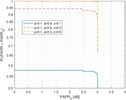
(a) PMEPR distribution ($m=8$).

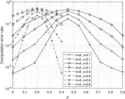
(b) CER in AWGN channel.

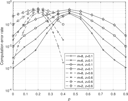
(c) CER in flat-fading channel.

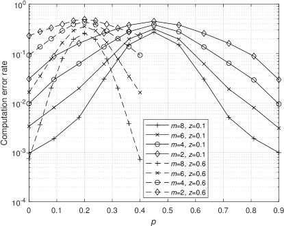
(d) CER in frequency-selective channel.

Figure 1: CER for in AWGN, flat-fading, and frequency-selective channels ($K=50$ sensors) and PMEPR distribution.

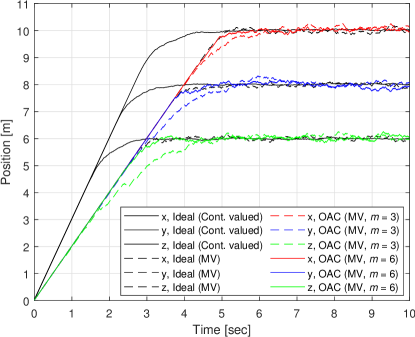
(a) UAV’s trajectory in time.

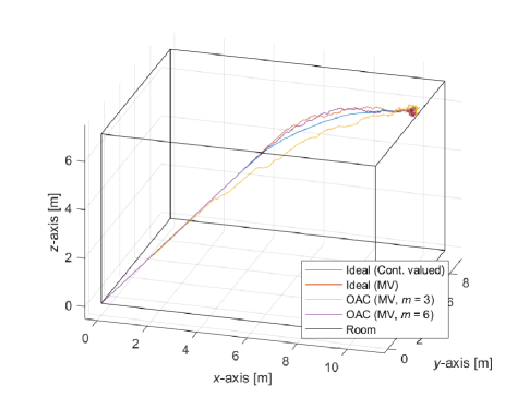
(b) UAV’s trajectory in space.

Figure 2: UAV’s trajectory with a single point of interest. The initial position is $(0,0,0)$ and the target position is $(10,8,6)$.

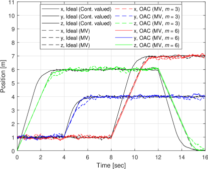
(a) UAV’s trajectory in time.

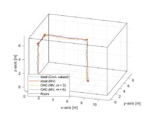
(b) UAV’s trajectory in space.

Figure 3: UAV’s trajectory with multiple points of interest, i.e., $(1,1,6)$, $(1,4,6)$, $(7,4,6)$, and $(7,4,0)$. The initial position is $(1,1,0)$.

In Figure 1, we provide the PMEPR distribution and the CER for a given $\{p,q,z\}$, where $p$, $q$, and $z$ denote the probabilities $\mathrm{Pr}\left({v_{k,n}>0}\right)$, $\mathrm{Pr}\left({v_{k,n}<0}\right)$, and $\mathrm{Pr}\left({v_{k,n}=0}\right)$, respectively, for $K=50$ sensors. In Figure 1LABEL:sub@subfig:pmepr, we provide PMEPR distribution for $m=8$, $p=0.1$ and $z\in\{0.1,0.3,0.6\}$. We show that the PMEPR of the proposed scheme is always less than or equal to $3$ dB due to the properties of the CSs. If there are no absentee votes, the maximum PMEPR of the proposed scheme is $0$ dB since a single subcarrier is used for the transmission. Hence, for a larger absentee vote probability, the probability of observing $0$ dB PMEPR increases. The combination of sequences that lead to $0$ dB and $3$ dB PMEPR values result in the jumps in the PMEPR distribution given in Figure 1LABEL:sub@subfig:pmepr. In Figure 1LABEL:sub@subfig:CERAWGN-LABEL:sub@subfig:CERselectiveFading, we analyze CER for $z\in\{0.1,0.6\}$ and $m=\{2,4,6,8\}$ by sweeping $p$ in AWGN (i.e., $h_{k,{i}}=1$), flat-fading (i.e., $h_{k,{i}}=h_{k,{i}^{\prime}}\sim\mathcal{CN}({0,1})$), and frequency-selective (i.e., $h_{k,{i}}\sim\mathcal{CN}({0,1})$) channels, respectively. We observe that the proposed scheme achieves a better CER for increasing $m$ at the expense of more resource consumption in all channel conditions. The CER improves for a small or a large $p$ since more sensors vote for $-1$ or $+1$, respectively. The performance in frequency selective channel is slightly better than the flat-fading channel because of the diversity gain.

In Figure 2 and Figure 3, we consider the distributed UAV guidance scenario discussed in Section II for $K=50$ sensors. We assume $T_{\mathrm{update}}=10$ ms, $\mu=2$, $u_{\text{\rm limit}}=3$ m/s, $\sigma_{\rm sensor}^{2}=2$, and ${\tt{SNR}}=10$ dB. We provide the trajectory of the UAV in time and space for the aforementioned waypoint flight control scenario. We consider two cases. In the first case, there is only one point of interest $({c}_{\mathrm{t},1},{c}_{\mathrm{t},2},{c}_{\mathrm{t},3})=(10,8,6)$ and the initial position of the UAV is $(0,0,0)$. In the second case, the points of interest are $(1,1,6)$, $(1,4,6)$, $(7,4,6)$, and $(7,4,0)$, where the initial position of the UAV is $(1,1,0)$. We compare the proposed scheme for $m\in\{3,6\}$ in a practical communication channel with both continuous and MV-based feedback in an ideal communication channel (i.e., no error due to the communications). As can be seen from Figure 2LABEL:sub@subfig:wayPointSingleTime, for the continuous-valued feedback, the UAV reaches its position faster than any MV-based approach. This is because the velocity increment is limited with the step size for MV-based feedback in our setup. Hence, as can be seen from Figure 2LABEL:sub@subfig:wayPointSingleSpace the UAV’s trajectory in space is slightly bent. Since the proposed scheme is also based on the MV computation, its characteristics are similar to the one with MV computation in an ideal channel. Since the CER with $m=6$ is lower than the one with $m=3$, the proposed scheme for $m=6$ performs better and its characteristics are similar to the ideal MV-based feedback. The position of the UAV in time and space for multiple points of interest is given in Figure 3LABEL:sub@subfig:wayPointTime and Figure 3LABEL:sub@subfig:waypointSpace, respectively. The proposed scheme for $m=6$ performs similarly to the one with the MVs in ideal communications and increasing $m$ leads to a more stable trajectory.

V Concluding Remarks

In this study, we modulate the amplitude of the CS based on Theorem 1 to develop a new non-coherent OAC scheme for MV computation. We show that the proposed scheme reduces the CER via bandwidth expansion in both flat-fading and frequency-selective fading channel conditions while maintaining the PMEPR of the transmited signals to be less than or equal to $3$ dB. We demonstrate the applicability of the proposed OAC scheme to an indoor flight control scenario and show that the proposed scheme performs similar to the case where MV without OAC with larger length of sequences. In the future work, we provide the theoretical computation error and convergence analyses for distributed UAV guidance.

References

• [1] M. Goldenbaum, H. Boche, and S. Stańczak, “Nomographic functions: Efficient computation in clustered Gaussian sensor networks,” IEEE Trans. Wireless Commun., vol. 14, no. 4, pp. 2093–2105, 2015.
• [2] A. Şahin and R. Yang, “A survey on over-the-air computation,” IEEE Communications Surveys & Tutorials, pp. 1–33, 2023.
• [3] B. Nazer and M. Gastpar, “Computation over multiple-access channels,” IEEE Trans. Inf. Theory, vol. 53, no. 10, pp. 3498–3516, Oct. 2007.
• [4] M. Goldenbaum, H. Boche, and S. Stańczak, “Harnessing interference for analog function computation in wireless sensor networks,” IEEE Trans. Signal Process., vol. 61, no. 20, pp. 4893–4906, 2013.
• [5] M. Chen, D. Gündüz, K. Huang, W. Saad, M. Bennis, A. V. Feljan, and H. Vincent Poor, “Distributed learning in wireless networks: Recent progress and future challenges,” IEEE J. Sel. Areas Commun., pp. 1–26, 2021.
• [6] A. Şahin, “Distributed learning over a wireless network with non-coherent majority vote computation,” IEEE Trans. Wireless Commun., pp. 1–16, 2023.
• [7] G. Zhu, Y. Wang, and K. Huang, “Broadband analog aggregation for low-latency federated edge learning,” IEEE Trans. Wireless Commun., vol. 19, no. 1, pp. 491–506, Jan. 2020.
• [8] G. Zhu, Y. Du, D. Gündüz, and K. Huang, “One-bit over-the-air aggregation for communication-efficient federated edge learning: Design and convergence analysis,” IEEE Trans. Wireless Commun., vol. 20, no. 3, pp. 2120–2135, Nov. 2021.
• [9] B. McMahan, E. Moore, D. Ramage, S. Hampson, and B. A. y. Arcas, “Communication-Efficient Learning of Deep Networks from Decentralized Data,” in Proc. International Conference on Artificial Intelligence and Statistics (AISTATS), A. Singh and J. Zhu, Eds., vol. 54.   PMLR, Apr 2017, pp. 1273–1282.
• [10] P. Park, P. Di Marco, and C. Fischione, “Optimized over-the-air computation for wireless control systems,” IEEE Commun. Lett., vol. 26, no. 2, pp. 1–5, 2022.
• [11] S. Cai and V. K. N. Lau, “Modulation-free M2M communications for mission-critical applications,” IEEE Transactions on Signal and Information Processing over Networks, vol. 4, no. 2, pp. 248–263, 2018.
• [12] J. Lee, Y. Jang, H. Kim, S.-L. Kim, and S.-W. Ko, “Over-the-air consensus for distributed vehicle platooning control (extended version),” 2022. [Online]. Available: https://arxiv.org/abs/2211.06225
• [13] X. Zeng, X. Zhang, and F. Wang, “Optimized UAV trajectory and transceiver design for over-the-air computation systems,” IEEE Open Journal of the Computer Society, pp. 1–9, 2022.
• [14] M. Fu, Y. Zhou, Y. Shi, C. Jiang, and W. Zhang, “UAV-assisted multi-cluster over-the-air computation,” IEEE Trans. Wireless Commun., pp. 1–1, 2022.
• [15] M. M. Amiri and D. Gündüz, “Federated learning over wireless fading channels,” IEEE Trans. Wireless Commun., vol. 19, no. 5, pp. 3546–3557, Feb. 2020.
• [16] H. Jung and S.-W. Ko, “Performance analysis of UAV-enabled over-the-air computation under imperfect channel estimation,” IEEE Wireless Commun. Lett., pp. 1–1, Nov. 2021.
• [17] S. S. M. Hoque and A. Şahin, “Chirp-based majority vote computation for federated edge learning and distributed localization,” IEEE Open Journal of the Communications Society, pp. 1–1, 2023.
• [18] M. Goldenbaum and S. Stanczak, “Robust analog function computation via wireless multiple-access channels,” IEEE Trans. Commun., vol. 61, no. 9, pp. 3863–3877, 2013.
• [19] A. Şahin and R. Yang, “A generic complementary sequence construction and associated encoder/decoder design,” IEEE Trans. Commun., pp. 1–15, 2021.
• [20] J. A. Davis and J. Jedwab, “Peak-to-mean power control in OFDM, Golay complementary sequences, and Reed-Muller codes,” IEEE Trans. Inf. Theory, vol. 45, no. 7, pp. 2397–2417, Nov. 1999.
• [21] E. Dahlman, S. Parkvall, and J. Skold, 5G NR: The Next Generation Wireless Access Technology, 1st ed.   USA: Academic Press, Inc., 2018.